Data linkage – further research and ways forward

Stephen McKay (Birmingham) and Simon Lunn (DWP)

22 June 2012

Overview

• FRS and benefit counts

• Data linkage

• Extent of agreement and mismatch

• Dealing with unlinked cases

• Evaluation of approaches

• Ways forward

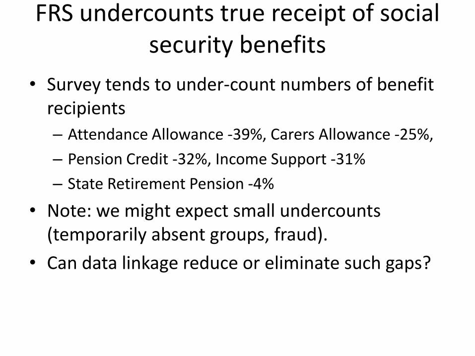
FRS undercounts true receipt of social security benefits

• Survey tends to under-count numbers of benefit recipients – Attendance Allowance -39%, Carers Allowance -25%,

– Pension Credit -32%, Income Support -31%

– State Retirement Pension -4%

• Note: we might expect small undercounts (temporarily absent groups, fraud).

• Can data linkage reduce or eliminate such gaps?

Rate of consent in FRS

• Just over 60% of those asked for linking agree, but only full respondents (not proxies) are asked. So, overall: – 52% provide consent to data linking;

– 30% per cent decline to provide consent;

– 18% information collected ‘by proxy’ and therefore not asked for consent. • Plus Northern Ireland excluded

Data linking issues – Income Support (IS)

Type of case FRS: receive IS FRS: £IS Admin: IS Admin: £IS

Linked, 100% accurate

Y £87.50 Y £87.50

Linked, wrong amount

Y £85 Y £88.50

Linked: false recipient

Y £30 N ..

Linked: hidden recipient

N .. Y £40

Unlinked case Y £95 ? ?

Unlinked case N .. ? ?

Unlinked case N .. ? ?

Extent of false and hidden recipients

Extent of mismatches [n=21,610] Benefit Admin and

survey data Only in admin

data Only in survey

data

Retirement Pension

6,079 46 312

Pension Credit 1,141 370 87

Attendance Allowance

436 263 63

Income Support 795 146 174

Jobseeker’s Allowance

459 149 133

Accuracy of benefit amounts

Bivariate analysis of bias II

Adults in household

Consenters Non-consenters

Proxies only

1 24 22 *

2 56 56 56

3 13 13 23

4+ 8 9 21

Bivariate analysis of bias II

Adults in household

Consenters Non-consenters plus proxies

1 24 14

2 56 56

3 13 17

4+ 8 14

Model of consent (logistic regression)

• Less likely among young (<30) and old (>=80)

• More likely in NE and Scotland, less likely in London

• More common among tenants than home-owners

• Less likely for self-employed, more likely for unemployed and economically inactive

• Less likely for non-white

• More common for 1-person households, less likely for larger households (where more proxies)

Tackling the missing data problem

Approaches to missing data

• Lumley (2010: 186) ‘Multiple imputation and survey reweighting are sometimes described as “statistically principled” approaches to inference with missing data’.

Missing Data Mechanisms

Missing Completely at Random (MCAR): • Consistent results with missing data can be obtained by

performing the analyses we would have used had there been no missing data

Missing at Random (MAR): • Given the observed data, the reason for the missingness

does not depend on the unobserved data Missing Not at Random (MNAR): • The reason for observations being missing still depends on

the unseen observations themselves

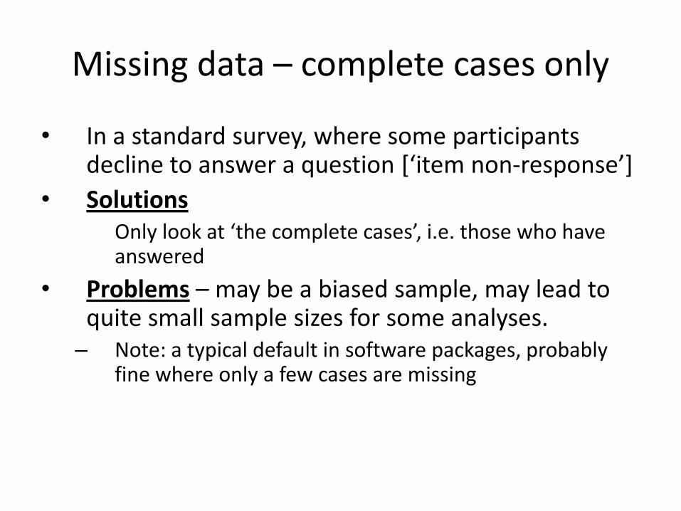
Missing data – complete cases only

• In a standard survey, where some participants decline to answer a question [‘item non-response’]

• Solutions Only look at ‘the complete cases’, i.e. those who have

answered

• Problems – may be a biased sample, may lead to quite small sample sizes for some analyses.

– Note: a typical default in software packages, probably fine where only a few cases are missing

Missing data – reweighting

• In a follow-up study, where some participants do not agree to a second interview stage [‘unit non-response’]

• Solution – re-weight the sample using the available data

• Problems – response may depend on new factor not captured at w1; weights may be diverse giving less ‘stable’ estimates; assumption of similarity of responders and non-responders (within response groups)

Missing data – imputation

• In a standard survey, where some participants decline to answer a question [‘item non-response’]

• Solutions Impute the non-responders’ data

• Problems – alternative approaches to imputation, how confident in the new values (and how to account for that in any analysis)

Imputation methods

• Single imputation – Mean-substitution – Regression imputation (deterministic or including a

random element) – Hot-deck imputation

• Multiple imputation – Generate M datasets with an imputation approach with a

random element (M typically 4-10) – Run models M times – Summarise results from set of those results – More about recovering correct model parameters than

finding the best replacement value for individuals • For specific tasks, not really for distributing a general-purpose

dataset

Selection models of bias in amounts of benefit (‘Heckman’ models)

• Heckman model includes in the regression a term (λ) representing selection probability

• e.g. look at bias in amounts reported, conditional on selection into consent status.

• Tends to find selection bias for most non-means-tested benefits, and not for most means-tested benefits (with exceptions).

• However, assumption of normality may be affecting this.

• Small changes in models can significantly alter these conclusions.

Approach to evaluation

• Detailed evaluation of consequences of each approach (including similarity to existing approaches, practicability, transparency)

• Other studies – – PASS-based studies that linked the non-consenters

• Little to choose between approaches • Small consent bias, compared with non-response issues or

‘measurement error

– Simulation study [Rebecca Landy] prefers multiple imputation to Heckman (mostly) on results and on practical grounds

• Comparison with aggregate data

Details of approaches used

• Re-weighting (‘grossing’): calibration weighting to gender, age group and region (Deville and Särndal 1992).

• Imputation: – hot-deck approach for amounts of benefit

(imputation classes based on reported receipt level).

– Imputing actual receipt status based on predictions from logistic regression model (finding ‘hidden recipients’ among non-consenters)

Caveats

• Based on a wide range of benefits and approaches

But

• Not all benefits, and not other sources of income (earnings, child support, non-state pensions)

• For one year of data

• Methods used were ‘proof of concept’

Average amount of benefit received

Benefit National data

(Aug-2009)

FRS data Admin & survey

Admin & imputed

Consenters only

Consenters re-

weighted

AA 60.03 57.26 58.14 58.46 58.76 58.77 PC 55.66 48.11 51.36 52.30 51.77 52.89 JSA 59.73 60.98 60.20 63.42 60.76 60.58 IS 84.61 73.53 80.10 83.50 82.29 82.53 RP 102.35 108.43 108.06 107.77 109.77 110.61 Total error (RMSE) – smaller is better

6.72 3.88 3.41 3.96 4.06

Note: weighted by gross3, apart from final column.

Regression model of receipt of AA

Results compared

• Approach based on swapping data for consenters, retaining survey data for non-consenters, is surprisingly robust despite its apparent inconsistency

• Consenters-only (whether or not re-weighted) performs least well in most scenarios – but a ‘complete cases’ approach may be a useful benchmark

• Issues about imputing receipt – works well for amounts of benefit, more controversial for actuality of receipt, but seems to work well.

• No approach is always best, though most do improve on the basic survey data.