DATA HANDLING IN SCIENCE AND TECHNOLOGY -VOLUME 4

Advanced scientific computing in BASIC with applications

in chemistry, biology and pharmacology

DATA HANDLING IN SCIENCE AND TECHNOLOGY

Advisory Editors: B.G.M. Vandeginste, O.M. Kvalheim and L. Kaufman

Volumes in this series:

Volume 1 Microprocessor Programming and Applications for Scientists and Engineers by R.R. Smardzewski

Volume 2 Chemometrics: A textbook by D.L. Massart, B.G.M. Vandeginste, S.N. Deming, Y. Michotte and L. Kaufrnan

Volume 3 Experimental Design: A Chemometric Approach by S.N. Deming and S.N. Morgan Volume 4 Advanced Scientific Computing in BASIC with Applications in Chemistry, Biology and

Pharmacology by P. Valk6 and S. Vajda

DATA HANDLING IN SCIENCE AND TECHNOLOGY -VOLUME 4

Advisory Editors: B.G.M. Vandeginste, O.M. Kvalheim and L. Kaufman

Advanced scientific computing in BASIC with applications in chemistry, biology and pharmacology

P. VALKO Eotvos Lorand University, Budapest, Hungary

S. VAJDA Mount Sinai School of Medicine, New York, N Y, U. S. A.

ELSEVIER

Amsterdam - Oxford - New York - Tokyo 1989

ELSEVIER SCIENCE PUBLISHERS B.V. Sara Burgerhartstraat 25 P.O. Box 2 1 1, 1000 AE Amsterdam, The Netherlands

Disrriburors for the United Stares and Canada:

ELSEVIER SCIENCE PUBLISHING COMPANY INC. 655, Avenue of the Americas New York. NY 10010, U.S.A.

ISBN 0-444-87270- 1 (Vol. 4) (software supplement 0-444-872 17-X) ISBN 0-444-42408-3 (Series)

0 Elsevier Science Publishers B.V., 1989

All rights reserved. No part of this publication may be reproduced, stored in a retrieval system or transmitted in ariy form or by any means, electronic, mechanical, photocopying, recording or otherwise, without the prior written permission of the publisher, Elsevier Science Publishers B.V./ Physical Sciences & Engineering Division, P.O. Box 330, 1000 AH Amsterdam, The Netherlands.

Special regulationsfor readers in the USA - This publication has been registered with the Copyright Clearance Center Inc. (CCC), Salem, Massachusetts. Information can be obtained from the CCC about conditions under which photocopies of parts of this publication may be made in the USA. All other copyright questions, including photocopying outside of the USA, should be referred to the publisher.

No responsibility is assumed by the Publisher for any injury and/or damage to persons or property as a matter of products liability, negligence or otherwise, or from any use or operation of any meth- ods, products, instructions or ideas contained in the material herein.

Although all advertising material is expected to conform to ethical (medical) standards, inclusion in this publication does not constitute a guarantee or endorsement of the quality or value of such product or of the claims made of it by its manufacturer

Printed in The Netherlands

I m I m ..................................................... VIII

1 1.1 1.1.1 1.1.2 1.1.3 1.1.4 1.2 1.2.1 1.2.2

1.3 1.3.1 1.3.2 1.3.3 1.3.4 1.4 1.5 1.6 1.7 1.8 1.B.1 1.8.2 1.8.3 1.8.4

1.8.5 1.8.6 1.8.7 1.8.0

2 2.1 2.1.1 2.1.2 2.1.3 2.1.4 2.1.5 2.1.6 2.2 2.2.1 2.2.2 2.3 2.3.1 2.3.2 2.3.3

D Y F U T A T I m LINPR CYGEBFW ...................................... Basic concepts and mett-uds ........................................ Linear vector spaces .............................................. Vector coordinates in a new basis ................................. Solution of matrix equations by Gauss-Jordan mliminatim .......... Matrix inversion by Gauss-Jordan eliminatim ...................... Linear programming ................................................ Simplex method for normal form .................................... Reducing general problenw to normal form . The two phase simplex method ............................................................ LU decomposition .................................................. Gaussian eliminatim .............................................. Performing the LU decomposition ................................... Solution of matrix equations ...................................... Matrix inversion .................................................. Inversion of symnetric, positive definite matrices ................ Tridiagonel systms of equations .................................. Eigenvalues and eigenvectors of a symnetric matrix ................ Accuracy in algebraic canpltatims . Ill-cmditimed problems ...... Applications and further problms ................................. Stoichianetry of chemically reacting species ...................... Fitting a line by the method of least absolute deviations ......... Fitting a line by minimax method .................................. Chalyis of spectroscopic data for mixtures with unknctm backgrcund absorption ........................................................ Canonical form of a quadratic response functim ................... Euclidean norm and conditim nhber of a square matrix ............ Linear dependence in data ......................................... Principal component and factor analysis ........................... References ........................................................ NELINAR EGWTIONS CYUD E X T E W I PRoBLDVls ......................... Nanlinear equations in m e variable ............................... Cardano method for cubic equatims ................................ Bisection ......................................................... False positim method ............................................. Secant method ..................................................... Newton-Raphsa, method ............................................. Successive approximatim .......................................... Minimum of functims in me d i m s i m ............................. Golden section search ............................................. Parabolic interpolation ........................................... Systems of nonlinear equatims .................................... Wegstein method ................................................... Newton-Raphsm method in multidimsims ..........................

1 2 2 5 9 12 14 15

19 27 27 28 32 34 35 39 41 45 47 47 51 54

96 59 68 61 65 67

69 71 71 74 77 00 82 85 87 88 96 99 W 104

Sroyden method .................................................... 107

VI

2.4 2.4.1 2.4.2 2.5 2.5.1 2.5.2 2.5.3 2.5.4

3 3.1 3.2 3.3 3.4 3.5 3.5.1 3.5.2 3.6 3.7 3.8 3.9 3.10 3.10.1

Minimization in multidimnsions ................................... 112 Simplex method of Nelder and Mead ................................. 113 Davidon-Fletcher-Powell method .................................... 119 Applications and further problems ................................. 123 Analytic solution of the Michaelis-l*lenten kinetic eqwtim ........ 123 Solution equilibria ............................................... 125 Liquid-liquid equilibrium calculation ............................. 127 Minimization subject to linear equality constraints chemical equilibrium composition in gas mixtures .................. 130 RefermcE ........................................................ 137

PMNCIER ESTIMCITIaV .............................................. Wltivariable linear regression ................................... Nonlinear least squares ........................................... Fitting a straight line by weighted linear regression .............

Linearization. weighting and reparameterization ................... Ill-conditioned estimation problems ............................... Ridge regression .................................................. Overparametrized nonlinear models ................................. kltirespmse estimation .......................................... Equilibrating balance equations ................................... Fitting error-in-variables models ................................. Fitting orthogonal polynomials .................................... Applications and further problems ................................. 0-1 different criteria for fitting a straight line .................

139 145 151 161 173 178 179 182 184

1BE 194 205 209 209

3.10.2 Design of experiments for parameter estimation .................... 210 3.10.3 Selecting the order in a family of homrlogous models .............. 213 3.10.4 Error-in-variables estimation of van Laar parameters fran vapor-

4 4.1 4.1.1 4.1.2 4.1.3 4.1.4 4.2 4.2.1 4.2.2 4.3 4.3.1 4.3.2 4.3.3 4.4 4.4.1 4.4.2

liquid equilibrium data ........................................... References ........................................................ SI(3rYy PRonSsING ................................................. Classical mthods ................................................. Interpolation ..................................................... Smmthing ......................................................... Differentiation ................................................... Integratim ....................................................... Spline functions in signal prccessing ............................. Interpolating splines ............................................. Smmthing splines ................................................. Fourier transform spectral methods ................................ Continuous Fourier transformation ................................. Discrete Fourier transformation ................................... Application of Fourier transform techniques ....................... Applications and further problem ................................. Heuristic methods of local interpolation .......................... Praessing of spectroscopic data .................................. References ........................................................

214 217

220 224 224 228 230 234 235 235 2416 246 247 249 252 257 257 258 2&0

VII

5 5.1 5.1.1 5.1.2 5.1.3 9.2 5.3 5.4 5.5 5.6 5.7 5.8 5.8.1 5.8.2

D W I W MWLS .................................................. rUunerical solution of ordinary differential e q w t i m s ............. Runge . Kutta methods ............................................. Adaptive step size control ........................................ Stiff differential equations ...................................... Sensitivity analysis .............................................. Estimation of parameterm in differential equations ................ Determining thh input of a linear system by numrrical deconvolutim Applications and furtkr problem ................................. Principal component analysis of kinetic models .................... Identification of a linear cunpartmntal model .................... References ........................................................

hltistep methods .................................................

Qmsi steady state approximation .................................. Identification of linear system ..................................

261 263 266 269 272 273 278 283 286 297 306 311 311 313 317

W E C T INDEX ..................................................... 319

VIII

INTRODUCTION

This book is a practical introduction to scientific computing and offers

BPSIC subroutines, suitable for use on a perscnal complter, for solving a

number of important problems in the areas of chmistry, biology and

pharmacology. Althcugh our text is advanced in its category, we assume only

that you have the normal mathmatical preparation associated with an

undergraduate degree in science, and that you have some familiarity with the

S I C programing language. We obviously do not persuade you to perform

quantum chemistry or molecular dynamics calculations on a PC , these topics are even not considered here. There are, however, important information -

handling needs that can be performed very effectively. A PC can be used to

model many experiments and provide information what should be expected as a

result. In the observation and analysis stages of an experiment it can acquire

raw data and exploring various assumptions aid the detailed analysis that turns

raw data into timely information. The information gained f r m the data can be

easily manipulated, correlated and stored for further use. Thus the PC has

the potential to be the major tool used to design and perform experiments,

capture results, analyse data and organize information.

Why do w e use

another programing language who challenge the use of anything else on either

technical or purely motional grounds, m t BASIC dialects certainly have

limitations. First, by the lack of local variables it is not easy to write

multilevel, highly segmented programs. For example, in FWTRAN you can use

subroutines as "black boxes" that perform 5 ~ e operations in a largely

unknown way, whereas programing in BASIC requires to open tl-ese black boxes

up to certain degree. We do not think, hOwever, that this is a disadvantage for

the purpose of a book supposed to teach you numerical methods. Second, BASIC

is an interpretive language, not very efficient for programs that do a large

amwnt of "number - crunching'' or programs that are to be run many times. kit

the loss of execution speed is compensated by the interpreter's ability to

enable you to interactively enter a program, immdiately execute it and see the

results without stopping to compile and link the program. There exists no more

convenient language to understand how a numerical method works. BASIC is also

superb for writing relatively small, quickly needed programs of less than llaaw

program lines with a minimvn programming effort. Errors can be found and

corrected in seconds rather than in hours, and the machine can be inmediately

quizzed for a further explanation of questionable answers or for exploring

further aspects of the problem. In addition, once the program runs properly,

you can use a S I C compiler to make it run faster. It is also important that

BASIC? Althcugh we disagree with strong proponents of one or

IX

on most PC’s BASIC is usually very powerful for using all re5Wrce5,

including graphics, color, sound and commvlication devices, although such

aspects will not be discussed in this book.

Why do we claim that cur text is advanced? We believe that the methods and

programs presented here can handle a number of realistic problw with the

power and sophistication needed by professionals and with simple, step - by - step introductions for students and beginners. In spite of their broad range of

applicability, the subrcutines are simple enwgh to be completely understood

and controlled, thereby giving m r e confidence in results than software

packages with unknown source code.

Why do we call cur subject scientific computing? First, w e as- that you,

the reader, have particular problems to solve, and do not want to teach you

neither chemistry nor biology. The basic task we consider is extracting useful

information fran measurements via mcdelling, simulatim and data evaluation,

and the methods you need are very similar whatever your particular application is.

More specific examples are included only in the last sections of each chapter

to show the power of some methods in special situations and pranote a critical

approach leading to further investigation. Second, this book is not a course in

numerical analysis, and we disregard a number of traditional topics such as

function approximation, special functions and numerical integration of k n m

functions. These are discussed in many excellent books, frequently with PASIC

subroutines included. You will find here, however, efficient and robust

numerical methods that are well established in important scientific

applications. For each class of problems w e give an introduction to the

relevant theory and techniques that should enable you to recognize and use the

appropriate methods. Simple test examples are chDsRl for illustration. Although

these examples naturally have a numerical bias, the dominant theme in this book

is that numerical methods are no substitute for poor analysis. Therefore, we

give due consideration to problem formlation and exploit every opportunity to

emphasize that this step not only facilitates your calculations, but may help

ycu to avoid questionable results. There is nothing mt-e alien to scientific

computing than the use of highly sophisticated numerical techniques for solving

very difficult problw that have been made 50 difficult only by the lack of

insight when casting the original problem into mathematical form.

What is in this book? It cmsists of five chapters. The plrpose of the

preparatory Chapter 1 is twofold. First, it gives a practical introduction to

basic concepts of linear algebra, enabling you to understand the beauty of a

linear world. FI few pages will lead to comprehending the details of the two -

phase simplex method of linear programing. Second, you will learn efficient

numerical procedures for solving simultaheous linear equations, inversion of

matrices and eigenanalysis. The corresponding subrcutines are extensively used

X

in further chapters and play an indispensable auxiliary role. chang the direct

applications we discuss stoichimtry of chemically reacting systems, robust

parameter estimation methods based on linear progrming, as well as elements

of principal component analysis.

Chapter 2 g i w s an overview of iterative methods of solving ncnlinear

equations and optimization problems of m e or several variables. Though the one

variable case is treated in many similar bcoks, wm include the corresponding

simple subroutines since working with them may help you to fully understand t h

use of user supplied subroutines. For solution of simultaneous nonlinear

equations and multivariable optimization problmns sane well established methods

have been selected that also amplify the theory. Relative merits of different

m e t W s are briefly discussed. As applications we deal with equilibrium

p r o b l w and include a general program for complting chemical equilibria of

gasems mixtures.

Chapter 3 plays a central role. It concerns estimation of parameters in

complex models fran relatively small samples as frequently encavltered in

scientific applications. To d m s t r a t e principles and interpretation of

estimates we begin with two linear statistical methods (namely, fitting a

line to a set of points and a subroutine for mrltivariable linear regression),

but the real emphasis is placed on nonlinear problems. After presenting a

robust and efficient general purpose nonlinear least squares -timation

praedure we proceed to more involved methods, such as the multirespmse

estimation of Box and Draper, equilibrating balance equations and fitting

error-invariables models. Thcugh the importance of the6e techniques is

emphasized in the statistical literature, no easy-twsc programs are

available. The chapter is concluded by presenting a subroutine for fitting

orthogonal polynomials and a brief swrv~ry of experiment design approaches

relevant to parameter estimation. The text has a numerical bias with brief

discussion of statistical backgrmd enabling you to select a method and

interpret rexllts. Sane practical aspects of parameter estimation such as

near-singularity, linearization, weighting, reparamtrization and selecting a

mdel from a harologous family are discussed in more detail.

Chapter 4 is devoted to signal processing. Through in most experiments w e

record 5om quantity as a function of an independent variable (e.g., time,

frequency), the form of this relationship is frequently u n k n m and the methods

of the previous chapter do not apply. This chapter gives a swrv~ry of classical

XI

techniques for interpolating, smoothing, differentiating and integrating such

data sequences. The same problems are also sold using spline functions and

discrete Fourier transformation methods. Rpplications in potentiaetric

titration and spectroscopy are discussed.

The first two sections of Chapter 5 give a practical introduction to

dynamic models and their numslrical solution. In addition to 5omp classical

methods, an efficient procedure is presented for solving systems of stiff

differential equations frequently encountered in chemistry and biology.

Sensitivity analysis of dynamic models and their reduction based on

quasy-steady-state approximation are discussed. The secaxl central problem of

this chapter is estimating parameters in ordinary differential quations. ch

efficient short-cut method designed specifically for

applied to parameter estimation, numerical deconvolution and input

determination. Application examples concern enzyme kinetics and pharmacokinetic

canpartmental modelling.

PC's is presmted and

Prwram modules and sample p r w r w

For each method discussed in the book you will find a W I C subroutine and

an example consisting of a test problem and the sample program we use to solve

it. k r main asset5 are the subroutines we call program modules in order to

distinguish than from the problem dependent user supplied subroutines. These

modules will serve you as building blocks when developing a program of ycur aw

and are designed to be applicable in a wide range of problem areas. To this end

concise information for their use is provided in remark lines. Selection of

available names and program line numbers allow you to load the modules in

virtually any cabinatim. Several program modules call other module(.). Since

all variable names consist of two characters at the most, introducing longer

names in your o w user supplied subroutines avoids any conflicts. These user

supplied subroutines start at lines 600, 700, OE0 and %El , depending on the need of the particular module. Results are stored for further use and not

printed within the program module. Exceptions are the ones corresponding to

parameter estimation, where we wanted to save you from the additional work of

printing large amxlnt of intermediate and final results. You will not find

dimension statements in the modules, they are placed in the calling sample

programs. The following table lists our program modules.

XI1

Table 1 Program mcdules

M10 M11

M14 M15

Ml6 M17 M1B

m M z l

Mn

Mz3

Mz4

M25

M26

m

M31

M32

M34

M36

M4QJ M41 M42

M45

MW

Vector coordinates in a new basis Linear programing two phase simplex method LU decanposition of a square matrix Solution of sirmltanecus linear equations backward substitution using LU factors Inversion of a positive definite symmetric matrix Linear equations with tridiagonal matrix Eigenvalues and eigenvectors of a symmetric matrix - Jacobi method Solution of a cubic equation - Cardano method Solution of a nonlinear equation bisection method Solution of a nmlinear equation regula falsi method Solution of a nonlinear equation secant method Solution of a nonlinear equation

Minirmm of a function of one variable method of golden sections Minimum of a function of one variable parabolic interpolation - Brent's method Solution of sirmltanmus equations X = G ( X )

Wegstein method Solution of sirmltanmus equations F(X)=0

Solutim of sirmltanmus equations F(X)=0 Broyden method Minimization of a function of several variables Nelder-Mead method Minimization of a function of several variables Davidonfletcher-Powell method Fitting a straight line by linear regression Critical t-value at 95 % confidence level kltivariable linear regression weighted least squares Weighted least squares estimation of parameters in multivariable nonlinear models Gauss-Newton-Marquardt method Equilibrating linear balance equations by least squares method and outlier analysis

Newton-Raphson method

Newton-Rapkon method

1002

l lm 14eW

1500 lM0 1702

1WIZI Zen0

21m

2200

2302

24m

25m

2 m

ma0

31m

3 m

34m

3 m 4 m 41m

4 m

45x3

mzizl

1044

1342 1460

1538

1656 1740

1938 2078

2150

2254

2354

2454

2540

2698

3074

3184

3336

3564

3794 4096 4156

4454

4934

5130

XI11

M52

M55

M.0

M6l M62 M63 M64

M65

M67

M70

M71

M72

M75

Fitting an error-in-variables model of the form F(Z,P)=RJ modified Patindeal - Reilly method Polynomial regression using Forsythe orthogonal polynomials Newton interpolations computation of polynomial coefficients and interpolated valws Local cubic interpolation 5-pint cubic smoothing by Savitzky and Golay Determination of interpolating cubic spline Function value, derivatives and definite integral of a cubic spline at a given point Determination of Maothing cubic spline method of C.H. Reinsch Fast Fourier transform Radix-2 algorith of Cooley and Tukey Solution of ordinary differential equations fourth order Wga-Uutta method Solution of ordinary differential equations predictor-corrector method of Milne Solution of stiff differential equations semi-implicit Wge-Kutta method with backsteps RosRlbrak-Gottwald-khnner Estimation of parameters in differential equations by direct integral method extension of the Himnelblau-Jones-Bischoff method

54m

5628

6054 61 56 6250 6392

6450

6662

6782

7058

7288

7416

8040

While the program modules are for general application, each sample program

is mainly for demonstrating the use of a particular module. To this end the

programs are kept as concise as possible by specifying input data for the

actual problem in the DFITA statements. TMs test examples can be checked

simply by loading the corresponding sample program, carefully merging the

required modules and running the obtained program. To solve your ow7 problems

you should replace DFITA lines and the user supplied subroutines (if

neecled). In more advanced applications the READ and DFITA statemeots may be

replaced by interactive input. The following table lists thp sample programs.

! DISKETTE, SUITABLE FOR MS-DOS COMPUTERS. THE DISKETTE CAN BE

ORDERED SEPARATELY. PLEASE, SEE THE ORDER CARD IN THE FRONT OF THIS BOOK. - I------

XIV

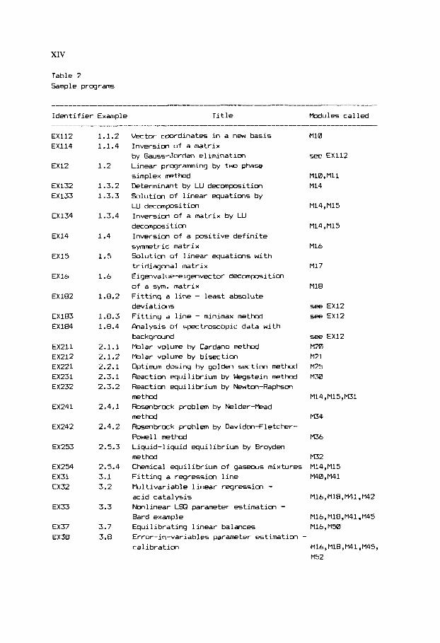
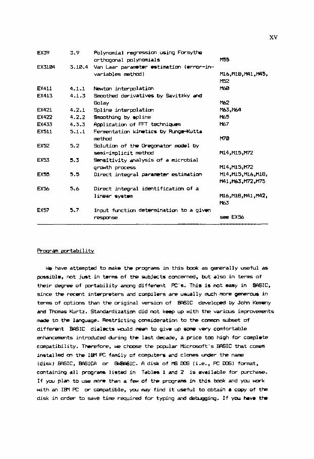
Table 2 Sample programs

Identifier Example Title Modules called

EX112 EX114

EX12

EX132 EX133

EX134

EX14

EX15

EX16

EX182

EX183 EX184

EX211 EX212 EX221 EX231 EX232

EX241

EX242

EX253

EX254 EX31 EX32

EX33

EX37 EX38

1.1.2 1.1.4

1.2

1.3.2 1.3.3

1.3.4

1.4

1.5

1.6

1.8.2

1.8.3 1.8.4

2.1.1 2.1.2 2.2.1 2.3.1 2.3.2

2.4.1

2.4.2

2.5.3

2.5.4 3.1 3.2

3.3

3.7 3.8

Vector coordinates in a new basis Inversion of a matrix by Gauss-Jordan elimination Linear programing by two phase simplex method Determinant by LU decomposition Solution of linear equations by LU decomposition Inversion of a matrix by LU

decomposition Inversion of a positive definite symmetric matrix Solution of linear equations with tridiagonal matrix Eigmvalue-eigmvector decomposition of a sym. matrix Fitting a line - least absolute deviations Fitting a line - minimax method Analysis of spectroscopic data with backgrwnd Molar volume by Cardano method Molar volume by bisection Optimm dosing by golden section method Reaction equilibrium by Wegstein method Reaction equilibrium by Newton-Raphsm method Rosenbrock problem by Nelder-Mead method Rosenbrock problem by Davidonfletcher- Powell method Liquid-liquid equilibrium by Broyden method

M1O

see EX112

M10, M11

M14

M14,M15

M14,M15

Mlb

M17

M18

see EX12 see EX12

see EX12 m M21 m5 M 3 0

M14,M15,MJ1

M34

M 3 6

M32 Chemical equilibrium of gasews mixtures M14,M15 Fitting a regression line M40, M41 Wltivariable linear regression - acid catalysis Ml6,MlB,M41,M42 Nonlinear Ls(3 parameter estimation - Bard example Mlb,MlB,M41,M45 Equilibrating linear balances Ml6,M50 Error-in-variables parameter estimation - calibration Mlb,MlB,M41,M45,

M52

EX39

EX3104

EX411 EX413

EX421 EX422 EX433 EX511

EX52

EX53

EX55

EX56

EX57

3.9

3.10.4

4.1.1 4.1.3

4.2.1 4.2.2 4.3.3 5.1.1

5.2

5.3

5.5

5.6

5.7

Polynomial regression using Forsythe orthogona 1 pol ynomial s Van Laar parameter estimation (error-in- variables method)

Newton interpdlatim Smmthed derivatives by Savitzky and Golay Spline interpolation Smoothing by spline Application of FFT techiques Fermentation kinetics by RungeKutta method Solutim of the Dregmator model by semi-implicit method Sensitivity analysis of a microbial growth process Direct integral parameter estimation

Direct integral identification of a linear system

Inplt function determination to a given respmse

MS5

Mlb,Ml8,M41,M45, M52 M60

M62

m,w M65 M67

m

M14 ,M15,M2

M14, M15, M2 M14,M15,Mlb,Ml8, M4l,M63,M72,M75

Mlb,M18,M41,M42, M63

see EX56

Prwram portability

We have attempted to make the programs in this b m k as generally useful as

possible, not just in terms of the subjects concerned, but also in terms of

their degree of portability among different

since the recent interpreters and compilers are usually much more generous in

terms of options than the original version of BASIC developed by J o h Kemeny

and Thomas Kurtz. Standardization did not keep up with the various improvmts

made to the language. Restricting consideration to the c m subset of

different W I C

enhancements introduced during the last decade, a price t m high for complete

compatibility. Therefore, we choose the popllar Microsoft’s WSIC that canes

installed on the IBM FC family of complters and clmes under the name

(disk) BASIC, BASICA or GWBASIC. A disk of Ms WS (i.e., PC WS) format,

containing all programs listed in Tables 1 and 2 is available for purchase.

If you plan to use more than a few of the programs in this b m k and you work

with an IBM PC or compatible, ycu may find it useful to obtain e copy of the

disk in order to save time required for typing and debugging. If you have the

PC’s. This is not easy in BASIC,

dialects would mean to give up sane very comfortable

XVI

sample programs and the program mcdules on disk, i t i s very easy t o run a test

example. For instance, t o reproduce Example 4.2.2 you should s t a r t your

BASIC , then load the f i l e "EX4Z.EAS", merge the f i l e "M65.EAS" and run the

program. I n order t o ease merging the programs they are saved i n ASCI I format

on the disk. You w i l l need a pr in ter since the programs are wr i t ten wi th

LPRINT statements. I f you prefer pr in t ing t o the screen, you may change a l l

the LFRINT statements t o PRIM statements, using the edi t ing f a c i l i t y of the

BASIC interpreter or the more user f r iendly change o p t i m of any edi tor

program.

Using our programs i n other BCISIC d ia lects you may experience sane

d i f f i cu l t i es . For example, several d ia lects do not allow zero indices of

an array, r e s t r i c t the feasible names of variables, give +1 instead of -1

for a logical expression i f i t i s true, do not allow the structure IF ... Tl€N

... ELSE, have other syntax fo r formatting a PRINT statement, etc. &cording

to our experience, the most dangerous ef fects are connected with the d i f ferent

treatment of FOR ... N X T Imps. In s ~ e versims of the language the

statements inside a l w p are carried out mce, even i f the I m p c c n d i t i m does

not allow it. I f running the following program

10 FOR 1.2 TO 1

28 PRINT "IF YOU SEE THIS, THEN YOU SHOULD BE CBREFUL WITH YOUR BASIC'

38 NEXT I

w i l l result i n no outpi t , then you have no r e a m t o worry. Otherwise you w i l l

f i nd i t necessary t o inser t a test before each FOR ... N X T loop that can be

mpty. For example, i n the module M15 the l w p i n l i n e 1532 i s mp ty i f

1 i s greater than K - 1 (i.e., K < 2) , tlus the l i n e

1531 I F C(2 THEN 1534

inserted i n t o the module w i l l prevent unpredictable results.

We deliberately avoided the use of sane elegant constructions as WILE ... WEND structure, SWAP statement, EN ERROR condition and never broke up a s ingle

s t a t m t i n t o several l ines. Although t h i s sel f - restraint implies that we had

to give up sane principles of structural programming (e.g., we used more GOT0

statements than i t was absolutely necessary), we think that the loss i s

conpensated by the improved po r tab i l i t y o f the programs.

XVII

Note to the reader

O f course we would be fool ish t o claim that there are no tugs i n such a

large number of program lines. We t r i ed t o be very careful and tested the

program modules m various problwm. Nevertheless, a new problem may lead t o

d i f f i c u l t i e s that we overlooked. Therefore, w e make no warranties, express or

implied, that the programs contained i n this book are free of error, or are

c m s i s t m t wi th any particular standard o f merchantibility, or that they w i l l

meet your requirements fo r any particular application. The authors and

publishers disclaim a l l l i a b i l i t y for d i rect or consquential damages resul t ing

from the use of the programs.

RK knowledsements

This book i s part ly based a7 a previous work o f the authors, published i n

Hvlgarian by Mszaki KMyvkiad6, Budapest, i n 1987. We wish t o thank t o the

editor of the Hvlgarian edition, D r J. Bendl, f o r his support. We also

grateful ly acknowledge the positive stimuli provided by Dr. P. Szepesvdry,

Prof. J.T. Clerc and cur colleagues and students a t the Eotvtis Lordnd

University, Budapest. While preparing the presmt book, the second author was

a f f i l i a t e d also with the Department of C h i s t r y a t Princeton Lhiversity, and

he i s indebted for the stimulating environment.

1

Chapter 1

COMPUTATIONAL LINEAR ALGEBRA

The problems we are going to study cans from chemistry, biology or

pharmacology, and most of them involve highly nonlinear relationships.

Nevertheless, there is almost no example in this book which could have been

solved withaut linear algebraic methods. MDreover, in most cases the success of

solving the entire problem heavily depends on the accuracy and the efficiency

in the algebraic compltation.

We assume most readers have already had xyne expoKlre to linear algebra, but

provide a quick review of basic concepts. ph usual, our natations are

X ” (1.1)

where x is the m-vector of the elements [xli, and A is the nwn matrix of

the elements CAIij = aij. Consider a scalar

m x p matrix B . The basic operations on vectors and matrices are defined as follows:

s, another ni-vector y, and an

where xTy i5 called the scalar product of x and y . We will also need the

Euclidean norm or simply the length of x , defined by 11x11 = ( X ~ X ) ” ~ . The most important canpltational tasks considered in this chapter are as

follows:

Solution of the matrix equation

2

& = b , (1.3)

where CI is an n m matrix of known coefficients, b is a know, right-hand

side vector of dimension n, and we want to find the m-vector x that

satisfies (1.3).

0 Calculatim of the matrix CI-' which is the matrix inverse of an n m

square matrix CI , that is

A-16 = m-1 = 1 , (1.4)

where I is the n m identity matrix defined by C1lij = 0 for i # j, and

CIIii = 1 .

0 Let a and b be vectors of dimension n. The inequality a 5 b means

ai 5 bi for all i = 1, ..., n. find the m-vector x which will maximize the linear function

In the linear programning problem w e want to

z = CTX (1.5)

subject to the restrictions

A x L b , x 2 0 .

As we show in Section 1.2, a more general class of problRm can be treated

similarly.

Solution of eigenvalue-eigenvector problem, where we find the eigenvalue h

and the eigenvector u of the square symmetric matrix CI such that

I % l = x u . (1.7)

These problem are very important and treated in many excellent books, for

example (refs. 1-61. Though the numerical methods can be presented as recipes,

i.e. , sequences of arithmetic operations, w e feel that their essmce wwld be

lost without fully understanding the underlying concepts of linear algebra,

reviewed in the next sectim.

1.1 BASIC W M P T S fW0 MTHJJX

1.1.1 Linear vector 50aces

The goal of this section is to extend 5ome cmcepts of 3dimensional space

$ to n dimensicns, and hence we start with $, the world we live in.

Considering the components ali,a21 and aS1 of the vector al = (all,a21,,a31) T

as cmrdinates, dl is show in Fig. 1.1. In terms of these cmrdinates

3

al = allel + a21q + aSl% , where ei denotes the i - t h unit vector defined

t

J

Fig. 1.1. Subspace i n J-dimmsional space

by Ceil = 1, Ceil = 0, i # j. I f s i s a scalar and 9 i s a vector i n

G, then 5al and a l+9 are also 3-dimensimal vectors, and the vector space

i s closed under rml t ip l icat ion by scalar5, and addition. This i s the

fundamental property of any l inear vector space. Consider the vectors and

9 i n Fig. 1.1, which are not on the same l ine. The set of l inear combinations

slal + s m , where s1 and s2 are arbi t rary scalars, i s a plane i n $. I f

bl and t~ are any vectors i n t h i s plane, then sbl and b1 + 9 are also i n

the plane, which i s therefore closed under m l t i p l i c a t i o n by scalars and

addition. Thus the plane generated by a l l l inear combinations of the form

slal + % chy vector i n th i s subspace i s of the form

described i n terms of the coordinates

system defined by the vectors a1 and 9 . We can, howwer, select another

system of coordinates (e.g., two perpendicular vectors of w i t length i n the

plane). I f al and 9 are coll inear, i.e., are m the same l ine, then the

combinations slal +

a1

i s also a l inear vector space, a Z-dimersional subspace of R3.

b = slal + % , and hence can be

b = (sl,s2IT i n the coordinate

define only this l ine, a one dimensional subspace of

R3. To generalize these well known concepts consider the n-vectors al, 9, ...,

a1 =

The linear combinations

. . ., q,,'

form a subspace of al, . . . ,a,,,. We face a number of questions concerning the structure of th is subspace. Do we

need a l l vectors al, 3, ..., a,,, be dropped? Do these vectors span the whole space R" ? How to choose a system

of coordinates i n the subspace? The an5wers to these questions are based on the

concept of linear independence. The vectors al, %, ..., q,, are said to be

l inearly independent i f the equality

I? which i s said to be spanned by the vectors

to span the subspace or sure of them could

slal + s* + ... + Sma, = 0 (1.10)

implies s1 = % = ... sm = 0 . Otherwise the vectors al, +, ..., q,, are said

to be l inearly dependent. In th is la t ter case w e can solve (1.10) such that a t

least me of the coefficients i s nmzero. Let

exwessed fran (1.10) as the linear combination

si # 0 , then ai can be

(1.11)

of the other vectors i n the system. I t i s ncw clear that we can res t r i c t

consideration to l inearly independent vectors when defining a subspace. ffisume

that there exists only r independent vectors m g al, *, ..., a,,,, i.e.,

any set of r+l vectors i s l inearly dependent. Then the integer r i s said to

be the rank of the vector system, and also define the dimension of the subspace

spanned by these vectors.

Let al,-, ...,a,- be a l inearly independent subset of vectors al,%, ...,am with rank r . Any vector i n the subspace can be expressed a5 a linear

canbination of

coordinate system i n the subspace, also called a.ba5is of the subspace. Since

any such set of r linearly independent vectors fo rm a basis, i t i s obviously

not unique.

q,-, ...,a,- , thus these la t ter can be regarded t o form a

I f r = n, then the l inearly independent vectors span the entire

5

1

0

el =

0

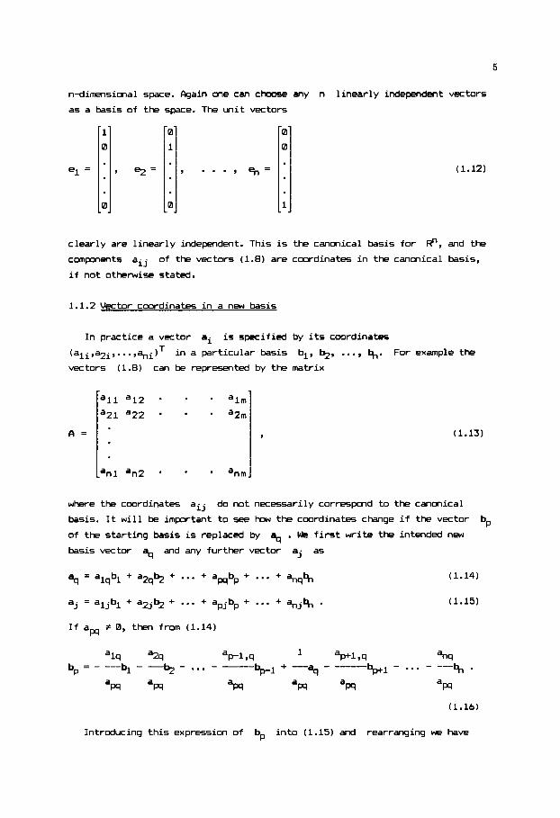
n-dimensional space. Again one can choose any n l inearly independent vectors

as a basis of the space. The uni t vectors

I

0

1

9 =

0

. ' (1.12)

clearly are l inearly independent. This i s the canonical basis for

components aij

i f not otherwise stated.

R", and the

of the vectors (1.8) are cmrdinates in the canonical basis,

1.1.2 Vector cmrdinates i n a new basis

In practice a vector ai i s specified by i t s cwrdinates

(ayi,a2i ,..., %iIT i n a particular basis bl, %, ..., %. For example the

vectors (1.8) can be represented by the m a t r i x

a l l a12

a21 a22

A = (1.13)

where the cwrdinates aij

basis. It w i l l be important t o see how the cmrdinates change i f the vector

of the starting basis i s replaced by

basis vector aq and any further vector a j as

do not necessarily correspmd to the canonical

bp % . We f i r s t write the intended new

(1.15)

Introducing th is expression of bp in to (1.15) and rearranging w e have

6

Since (1.17) gives aj as a l inear combination of the vectors

bl, 9 ,..., brl, $, bW1 ,..., b,, , i t s coeff ic ients

(1.18)

are the coordinates of aj i n the new basis. The vector bp can be replaced

by q i n the basis i f and only i f the pivot elwnent (or pivot) am i s

nonzero, since th i s i s the element we div ide by i n the transformations (1.113).

The f i r s t BASIC program module of t h i s book performs the coordinate

transformatims (1.18) when one of the basis vectors i s replaced by a new me.

Program d u l e M10

I880 REH t t t t t t l t t t t t t t t ~ ~ t ~ ~ ~ & t k t t k k k l t l t ! ~ t t l t t t ~ t ~ t ~ t : t t t 1082 REM $ VECTOR COORDINRTES 1N R NEW BRSlS : 1004 REH t l t l t t t t t ~ t t t t t t t t t t t t t ~ ~ t t I t k t t t t & t t t ? t ~ ? t t ! t t t t t t l00b RE! INPUT: 1808 REH N DlHENSION OF VECTORS I010 RER ti NUNBER OF VECTORS 1812 REH IP ROW INDEX OF THE PIVOT 1814 REfi JP COLUHN INDEX OF THE PIVOT 1016 REH I l N , N ) TABLE OF VECTOR COORDINATES 1018 REH OUTPUT: 1 0 2 0 REH A(N,M) VECTOR COORDINlTES IN THE NEW BASIS 1022 A=A(IP,JP) 1024 FOR J=I TO N :R(IP,J)=RIIP,J)/A :NEXT J 1026 FOR 1.1 TO N 1 0 2 8 IF I = I P THEN 1838 1838 A=AlI,JP) :IF A=8 THEN 1038 1832 FOR J=I TO n

i03e NEXT I

1834 1036 NEXT J

1 8 4 0 BI8,R(IP,0))=0 :A(IP,B)=JP :A(E,JP)=IP 1842 RETURN 1844 REH F t t l t t t t t t t t t t t t t t t t ~ t t t t t k ~ t t t t ~ t t t ~ t t ~ t t t t ~ t t ~ t t I

IF R ( I P , J I 0 9 THEN A 1 1, J I+.( 1, J I-R(IP ,J ) tA

The vector cmrdinates (1.13) occupy the array A(N,M). The module w i l l

replace the IP-th basis vector by the JP-th vector of the system. The pivot

element i s A(IP,JP). Since the module does not check whether A(IP,JPI i s

nmzero, yar should do th i s when selecting the pivot. The information on the

current basis i s stored i n the mtries A(0,J) and A(I,0) as follows:

0 if the I-th basis vector is ei

J if the I-th basis vector is aj A(I,0) = {

-2 1

1 2

- 5 , a 5 = -1 3

-7 2

0 if aj is not present in basis

I if aj is the I-th basis vector. A(0,J) =

l , d 6 '

The entry A(0,0) is a dumny variable.

If the initial coordinates in array A correspond to the canonical basis,

we set A(I,0) = A(0,J) = 0 for all I and J . Notice that the elements A(0,J) can be obtained from the values in A(1,0), thus we store redundant

information. This redundancy, however, will be advantageous in the programs

that call the d u l e M10.

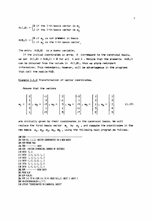
Example 1.1.2 Transformation of vector coordinates.

2

-1

3

1

5

kwne that the vectors

, a q = (1.19)

are initially given by their coordinates in the canmical basis. We will

replace the first basis vector el by al , and compute the coordinates in the new basis al, 9, %, e4, % , using the following main program as follows. 188 REH ________________________________________--------------- 182 REH EX. 1.1.2. VECTOR COORDINATES IN A NEW BASIS 104 RE! flER6E H I E 106 REM ---------- DATA I88 RE! (VECTOR DIHENSION, NUHBER OF VECTORS) 118 DATA 5, 6 112 DATA 2,-1, 2 , - 2 , 1, 1 114 DATA I, Z,-l, 1, 2, 3 I16 DATA -1,-2, 3,-5, 1, 2 118 DATA 3, 1, l ,-l, 3, 4 128 DATA 1,-3, 5,-7, 2, 3 288 REH ---------- READ DATA 202 READ N,il 284 DIM A[N,N) 206 FOR I=l TO N :FOR J+I TO H :READ A(I,J) :NEXT J : N E H I 288 V(=STRIN6$(Bt(Htl) , * - " ) 210 LPRINT 'COORDINATES I N CANONICAL BASIS'

8

PRINT COORDINATES 112 REH _ _ _ _ _ _ _ _ _ _ 214 LPRINT V1 216 LPRINT 'vector 1'; 218 FOR J=1 TO R :LPRINT TAB(Jt8t41;J; :NEWT J :LF'RINT 228 LPRINT ' i basis' 222 LPRINT V1 224 FOR 1.1 TO N 226 K=A(I,B) 228 IF K)0 THEN LPRINT USING " t a# ' ; l , K ; ELSE LPRINT USING" I. e t ' ; I , ] ; 238 FOR J = 1 TO ll :LPRINT USING ' t#t.t##';A(I,J); :NEXT J :LPRINT 232 NEWT I 234 LPRIHT V1 :LPRIHT

SELECT MODE 236 RER _ _ _ _ _ _ _ _ _ _ 238 INPUT 't(transforiation),r(row interchange) or 5(5topI';A$ 248 M=CHR1(32 OR A S C i A O l 242 IF A1:'t' THEN 246 ELSE I F A1='r" THEN 268 2114 I F A$='S' THEN 276 ELSE 238 246 RER ---------- TRANSFORHATION 248 INPUT 'row index ( I P ) and column index ( JP) o f the pivot: ' ; IP,JP 258 IF I P i l OR 1P)N OR JP(1 OR J P M THEN PRINT 'unfeasible* :GOTO 236 252 IF RBS(A[IP,JP))).BBB08~ 1HEN 256 254 PRINT 'zero or near ly 2ero pivot' :GOTO 236 256 LPRINT 'PIVOT R0W:';IP;" C0LUnN:';JP 258 GOSUB I888 :60TO 212 268 RER ---------- CHANGE TWO ROWS 262 INPUT "enter il,i2 to interchange row5 il and i2' ;11,12 264 IF II(1 OR I l > N OR 12(1 OR 12)N THEN PRINT 'unfeasible' :GOTO 236 266 IF A(II,8)4 OR A(I2,8)=0 THEN PRINT 'unfeasible" :6OTO 236 268 LPRINT 'ROWS INTERCHANGED:';I1;',';12 278 FOR J-8 TO H :R=RIll,J) :A(II,J)=A(I2,J) :8(12,J)=A :NEXT J 272 A(B,A( II ,8) )=I1 : A ( B , A ( 12,8) 1.12 274 GOT0 212 276 REH ---------- STOP 278 STOP

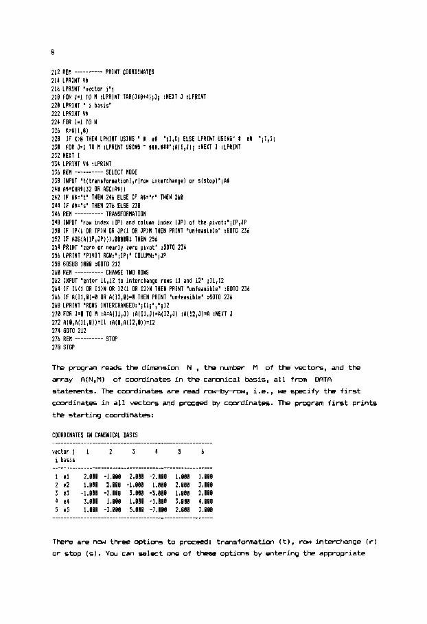
The program reads the dimension N , the number M of the vectors, and the

array FI(N,M) of coordinates i n the canonical basis, a l l f rom CAT0

statements. The coordinates are read rowby-row, i.e., w e specify the f i r s t

coordinates i n a l l vectors and proceed by coordinates. The program f i r s t prints

the starting cwrdinates:

COORDINATES I N CANONICAL BASIS

v e c t o r j 1 2 3 4 5 6 i basis

I e l 2.888 -1.888 2.888 -2.888 1.800 1.RBB 2 e2 1.888 2.888 -1.008 1.008 2.888 3.880 3 e3 -1.008 -2.808 3.888 -5.888 1.888 2.888 4 e4 3.988 1.880 1.888 -1.888 3.880 4.880 5 e5 1.880 -3.880 5.888 -7.808 2.888 3.888

........................................................

There are now three options to proceed: transformation ( t) , row interchange (r)

or stop (5). You can select me of these options by entering the appropriate

9

character.

In this example we perform a transformation, and hence enter "t". Then the

row index and the c o l m index of the pivot e1-t are required. We enter

"1,l" and the program returns the new coordinates:

PIVOT ROW: 1 COLUMN: 1

vector j I 2 3 4 5 6

........................................................

i basis

1 a1 1.008 -0.580 1.008 -1.008 8.580 0.580 2 e2 8.008 2.588 -2.008 2.888 1.508 2.588 3 e3 8.000 -2.500 4,808 -6.008 1.580 2.508 4 e4 8.008 2.508 -2.0UU 2.88B 1.500 2.588 5 e5 0.888 -2.500 4.800 -6.886 1.500 2.588

........................................................

........................................................

1.1.3 Solution of matrix wuations by Gauss-Jordan elimination

To solve the simltancus linear equations

A x = b (1.20)

recall that the coefficients in A can be regarded as the coordinates of the

vectors q,+, ...,a,,, (i.e., the colunns of A ) in the canonical basis.

Therefore, (1.20) can be written as

X1al + X A + ... + xm% = b (1.21)

with unknown coefficients

and only if b is in the subspace spanned by the vectors al,*, ...,a,, i.e., the rank of this system equals the rank of the extended system al,%, . . . ,a,,b.

For simplicity aswme first that A is a square matrix (i.e., it has the

same number n of rows and colms), and rank(A) = n. Then the c o l m s of A

form a basis, and the coordinates of b in this basis can be found replacing

the vectors el,% ,..., % by the vectors q,q, ..., q, , one-by-one. In this

new basis matrix A is the identity matrix. The procedure is called

Gauss-Jordan elimination. Fk we show in the following example, the method also

applies if n # m .

xl, xZ, ..., xm - There exist such coefficients if

Example 1.1.3 General solution of a matrix equation by Gauss-Jordan

elimination

Find all solutions of the sirmltaneous linear equations

10

2x1 -x2 +2x3 -2x4 +x5 = 1

x1 +zx2 -x3 +x4 +Zx5 = 3

-xl - 2 9 +3x3 -5x4 +x5 = 2

3Xl +x2 +x3 -x4 +3x5 = 4

x1 -3x2 +5x3 -7x4 +Zx5 = 3

(1.22)

The colurms of the coefficient matrix A i n eqn. (1.22) are the vectors

al, 9, %, a4, and i n (1.191, whereas the right-hand side b equals d6'

Therefore the problem can be solved by replacing further vectors of the current

basis i n the previous example. Replacing 9 by 9 and then 9 by we

obtain the following coordinates:

PIVOT ROW: 2 COLUHN: 2

v e c t o r j I 2 3 4 5 6 i basis

1 a 1 1.000 0.008 0.600 -8.680 0.800 1.088 2 a 2 0.080 1.908 -0.800 0.BBB 0.600 1.088 3 e3 0.000 0.000 2.000 -4.080 3.000 5.088 4 e4 0.008 0.000 0.0N0 'd.BB8 0.600 0.808 5 e5 0.000 0.080 2.008 -4.800 3.800 5.808

PIVOT ROW: 3 COLUIIN: 3

v e c t o r j I 2 3 4 5 b i basis

........................................................ I a1 1.000 0.000 0.000 9.600 -8.100 -8.508

3 a3 0.600 8.880 1.808 -2.010 1.588 2.580 2 a2 0.898 1.600 0.600 -0.800 1.886 3.880

4 e4 0.908 8.800 0.000 8.080 0.098 8.008 5 e5 0.080 0 . W 0.000 8.010 0.880 6.608

According to th is last table, the vectors a4 ,9 and a6 are expressed as

linear combinations of the vectors al,+ and 9 of the current basis. Thus

the rank of the coefficient m a t r i x of eqn. (1.22) and the rank of the extmded

system (1.19) are both 3, and we need only to interpret the results. From the

last c o l m of the table

ah = b = -0.5al + + 2.% , (1.23)

and hence x = (-0.5, 3, 2.5, 0, O)T

general solution, i.e., the set of a l l solutions, w e w i l l exploit that

i s a solution of (1.22). To obtain the

a4 and

are also givm i n terms of the f i r s t three vectors:

a4 = 0.6al - 0.- - 2%

9 = *.lal + 1.- + 1.* . (1.24)

(1.25)

11

Chmsing arbitrary values for x4 and x5 , eqns. (1.23-1.25) give

b = (-0.5 - 0 . 6 ~ ~ + 0.1x5)al + (3 + 0.8~~ - 1.8x5)q + (2.5 + 2x4 - 1.5X5)5 +

+ x4a4 + X5% . (1.26a)

Therefore, the general solution is given by

x1 = -0.5 - 0 . 6 ~ ~ + 0 . 1 ~ ~

x2 = 3 + 0 . 8 ~ ~ - 1 . 8 ~ ~

x3 = 2.5 + 2x4 - 1 . 5 ~ ~ . ( 1.26b)

Since (1.26b) gives the solution at arbitrary x4 and x5 , these are said to be "free" variables, whereas the coefficients xl, x2 and x3 of the

current basis vectors a 1, 9 and 5 , respectively, are called basis variables. Selecting another basis, the "free" variables will be no m r e

and x5, and hence we obtain a general solution that differs from

Emphasize that the set of solutions x is obtained by evaluating (1.26) for

all values of the "free" variables. Though another basis gives a different

algebraic expression for x , it may be readily verified that we obtain the

same set of values and tl-us the general solution is independent of the choice

of the basis variables.

x4 (1.26). We

In linear programming problwm we will need special solutions of matrix

equations with "free" variables set to zero. Th6?se are called basic solutions

of a matrix equation, where rank(&) is less than the number of variables.

The coefficients in (1.23) give such a basic solutim. Since in this example

the two "free" variables can be chosen in [:] = 10 different ways, the

equation m y have up to 10 different basic solutions.

In Examples 1.1.2 and 1.1.3 we did not need the row interchange option of

the program. This option is useful in pivoting, a practically indispensable

auxiliary step in the Gauss-Jordan pradure, a5 will be discussed in the next

sxtion. While the Gauss-Jordan procedure is a straightforward way of solving

matrix equations, it is less efficient than sure methods discussed later in

this chapter. It is, howwer, almost a5 efficient as any other method to

calculate the inverse of a matrix, the topics of our next section.

Exercises

0 Select a different basis in Example 1.1.3 and show that the basic solution

corresponding to this basis can be obtained from

of x4 and x5.

(1.26) as suitable values

Replace the last e l m t of the right-hand side vector b in (1.24) by 4.

12

We will run into trouble when trying to solve this system. Why?

1.1.4 Matrix inversion bv Gauss-Jordan elimination

Cmsider the n% square matrix A and find its inverse A-l defined by

M-l= I . (1.27)

Let Si = (Zli,Z2i,...S,.,i)T denote the i-th colunn vector of 0-l (i.e., the

set of cmrdinates in the canonical basis), then by (1.27)

where ei is the i-th unit vector. According to (1.28), the vector li is

given by the coordinates of the unit vector ei in the basis a l , S , ...,a, the colunn vectors of A . Thus we can find A-1 replacing the canonical

vectors el,%, ...,+ by the vectors al,*, ...,a,, in the basis one-byme.

In this new basis A is reduced to an identity matrix, whereas the coordinates

of el,% ,..., e,, form the c o l m s of A-' . If rank(A) < n , then A is said

to be singular, and its inverse is not defined. Indeed, we are then unable to

replace all unit vectors of the starting basis by the c o l m s of A .

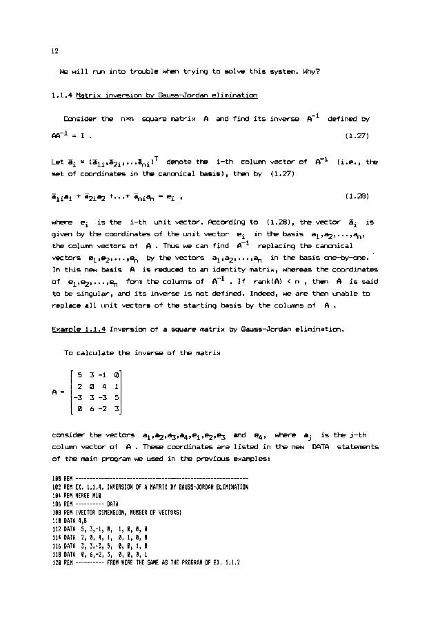
Example 1.1.4 Inversion of a square matrix by Gauss-Jordan elimination.

To calculate the inverse of the matrix

5 3-1 0

2 0 4 1

-3 3 -3 5

0 4-2 3

A =

consider the vectors a l , ~ , ~ , a 4 , e l , ~ , ~ and e4, where aj is the j-th

colunn vector of A . These coordinates are listed in the new DATA statements

of the main program we used in the previous examples:

188 RE\ ________________________________________-------------------- 102 REM EX. 1.1.4. INVERSION OF A IIATRIX BY GAUSS-JORDAN ELMINATION 104 REM IIERGE Hl8 106 REM ---------- DATA 188 REII (VECTOH DIHENSION, NUMBER OF VECTORS) 118 DATA 4,8 112 DATA 5, 3,-1, 0, 1, 0, 0, 0 114 DATA 2, 8, 4, I , 8, 1, 0, 0 116 DATA -3, 3 , -3 , 5, 0, 0, 1, 0 118 DATA 0 , 6,-2, 3, 8, 8, 8, 1 128 REH ---------- FRDN HERE THE SAHE AS THE PROGRAH OF EX. 1.1.2

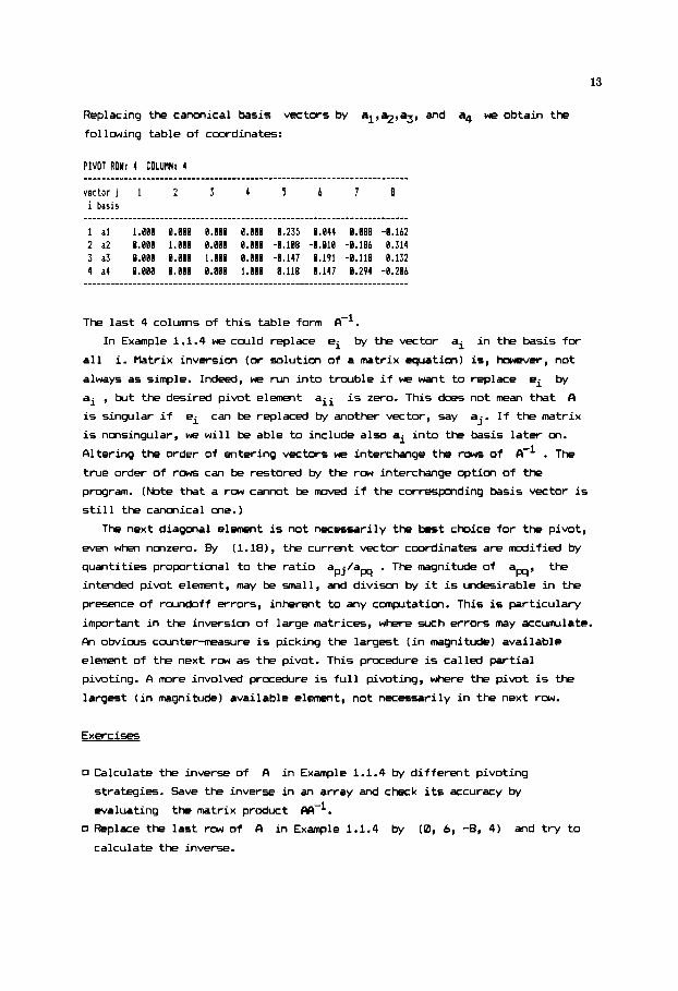
13

Replacing the canonical basis vectors by al,%,%, and a4 we obtain the

following table of coordinates:

P I V O T ROW: 4 COLUMN: 4

vector j 1 2 3 4 5 6 7 8 i basis

1 a1 1.880 8.888 8.888 8.888 8.235 8.044 0.888 -0.162 2 a2 8.0B8 1.088 8.888 8.008 -8.108 -0.010 -0.186 0.314 3 a3 8.880 0.800 1.880 8.888 -8.147 8.191 -8.118 0.132 4 a4 8.800 8.80B #.RE0 1.088 0.118 8.147 0.294 -0.206

The last 4 colwrns of th is table form A-'.

In Example 1.1.4 we could replace ei by the vector ai i n the basis for

a l l i. Matrix inversion (or solution of a m a t r i x equation) is , hcwever, not

always as simple. Indeed, w e run in to trouble i f we w a n t to replace ei by

ai , but the desired pivot element aii i s singular i f ei can be replaced by another vector, say aj. I f the m a t r i x

i s nmsingular, we w i l l be able to include also ai in to the basis later on.

Altering the order of entering vectors we interchange the rows of

true order of row5 can be restored by the row interchange option of the

program. (Note that a row cannot be mwed i f the correspmding basis vector i s

s t i l l the canonical me.)

i s zero. This does not mean that CI

CI-' . The

The next diagonal element i s not necessarily the best choice for the pivot,

even when nonzero. By (1.18), the current vector coordinates are mdi f ied by

quantities proportional to the rat io apj/aw . The magnitude of aw, the

intended pivot e l m t , may be small, and divison by i t i s undesirable i n the

presence of roundoff errors, inherent to any cmpltat im. This i s particulary

important i n the inversion of large matrices, where such errors may accumulate.

Fh obvious ccuntermeasure i s picking the largest ( i n magnitude) available

element of the next row as the pivot. This procedure i s called part ial

pivoting. A m r e involwd procedure i s f u l l pivoting, where the pivot i s the

largest ( i n magnitude) available element, not necessarily i n the next rcw.

Exercises

0 Calculate the inverse of A i n Example 1.1.4 by different pivoting

strategies. Save the inverse i n an array and chRk i t s accuracy by

evaluating the matrix product m-1. 0 Replace the last row of A i n Example 1.1.4 by (0, 6, -8, 4) and t r y to

calculate the inverse.

14

We begin by solving a simple blending problem, a classical example i n l inear

programing.

To kinds of row materials, A and B , are used by a manufacturer t o

produce products I and 11. To obtain each u n i t of product I he blends 1/3 u n i t

of A and 2/3 u n i t of B , whereas fo r each unit of product I 1 he needs 5/6

unit of A and 1/6 unit of B . The available supplies are 30 un i t s of A and

16 unit5 of B . I f the p r o f i t on each unit of product I i s 102 ECU (European

Currency Unit ) and the p r o f i t on each unit of product I 1 i s Z0 EUJ, how many

uni ts of each product should be made t o maximize the p ro f i t ?

Let x1 and x2 denote the number of un i ts of product I and 11,

respectively, being produced. By the l imi ted supply of A w e rmst have

whereas the supply of B gives

I n addition, the number of unit5 o f a product must be nonnegative:

x1 2 0, x2 2 0 .

z = lmxl + m x 2

(1.29c)

Now we want t o maximize the objective function (i.e., the p r o f i t ) given by

(I.=) subject t o the constraints (1.29).

Fk shown i n Fig. 1.2 , t o solve t h i s problem we need only analytical

geometry. The constraints (1.29) r e s t r i c t the solution t o a cmvex polyWron

i n the positive quadrant of the cwrdinate system. Any point of t h i s region

sat is f ies the inequalit ies

or feasible Mlut ion. The function (1.m) t o be maximized i s represented by

i t s contour lines. For a part icular value of z there exists a feasible

solution i f and only i f the contour l i n e intersects the region. Increasing the

value of z the contcur l i n e moves upmrd, and the optimal solution i s a

vertex of the polyhedron (vertex C i n t h i s example), unless the contour l i n e

w i l l include an ent i re segment of the bcundary. In any case, however, the

problem can be solved by evaluating and comparing the objective function a t the

vertices of the polyhedron.

(1.29), and hence corresponds t o a feasible vector

To f ind the cmrdinates of the vertices i t i s useful t o translate the

inequality constraints (1.29a -1.29b) i n t o the equal i t ies

1 5 = 3 0 5"1 + ax2 + x3

( 1.31a)

2 1 5 x 1 + ax2 + x4 = 16 (1 .Jib)

15

by introducing the so called slack variables xJ and x4 which mst be also

nonnegative. Hence (1.2%) takes the form

x1 2 0, x2 2 0, XJ 2 0, x4 2 0 . ( 1.31~ )

Fig. 1.2. Feasible region and contour lines of the objective function

The slack variables do not influence the objective function (1.m) but for

convmimce we can include them with zero coefficients.

We consider the equality cmstraints (1.31a-1.31b) as a matrix equation,

and generate one of its basic solution with "free" variables beeing zero. A

basic solution is feasible if the basis variables take nonnegative values.

It can be readily verified that each feasible basic solution of the matrix

equation (1.31a-1.31b) corresponds to a vertex of the polyhedron shown in

Fig. 1.2. Indeed, x1 = x2 = 0 in point A , x1 = x3 = 0 in point B , x3 = x4 = 0 in point C , and x2 = i4 = 9 .in p0int.D . This is a very, _ ,

important observation, fully exploited in the next section.

1.2.1 Simplex method for normal form

By introducing slack variables the linear programing problem (1.5-1.6)

can be translated into the normal form

16

Ax = b , ( b 2 0

x 2 0 ,

2 = CTX --> max , (1.32)

where we have n constraints, m+n variables and A denotes the (extended)

coefficient matrix of dimensions nx(m+n). (Here w e assume that the right-hand

side is nonnegative - a further assumption to be relaxed later on.) The key to

solving the original problem is the relationship bet- the basic solutions of

the matrix equation Ax = b and the vertices of the feasible polyhedron. Pn

obvious, but far from efficient procedure is calculating all basic solutions of

the matrix equation and comparing the values of the objective function at the

feasible ones.

The simplex algorith (refs.7-8) is a way of organizing the above

procedure rmch more efficiently. Starting with a feasible basic solution the

praedure will move into another basic solution which is feasible, and the

objective function will not decrease in any step. These advantages are due to

the clever choice of the pivots.

A starting feasible basic solution is easy to find if the original

constraints are of the form (1.6) with a nonnegative right-hand side. The

extended coefficient matrix A in (1.32) includes the identity matrix (i.e.,

the colwms of A corresponding to the slack variables xm+1, ..., xm. 1

Ccnsider the canonical basis and set xi = 0 for i = l,...,m, and x ~ + ~ = bi

for i = l,..,n. This is clearly a basic solution of Ax = b , and it is feasible by the assumption

know the coordinates of all the vectors in this basis. As in Section 1.1.3 , we

consider the right-hand side b as the last vector % = b, where M = m+n+l .

bi 2 0 . Since the starting basis is canonical, we

To describe me step of the simplex algorithn assume that the vectors

present in the current basis are

notation because the indices El, BZ, ..., Bn are changing during the steps of

the algorithn. They can take values from 1 to m+n . Similarly, we use the

notation cBi for the objective function coefficient corresponding to the

i-th basis variable. Assume that the current basic solution is feasible, i.e,

the coordinates of 4.1 operations to perform:

%, ..., %. We need this indirsct

are nonnegative in the current basis. We first list the

(i) Complte the indicator variables zj - cj for all j = 1, ..., m+n where z j is defined by

n (1.33)

-77 zj = 2, a. .c '

1J Ell . i=l

The expression (1.33) can be complted also for j = M. In this case it

17

gives the current value of the objective function, since the "free"

variables vanish and aim is the value of the i-th basis variable.

(ii) Select the column index q such that zq - c < z . - c . for all 9 - J J j = 1, ..., m+n, i.e., the column with the least indicator variable

value. If

proceed to step (iii).

zq - cq 2 0 , then we attained the optima1 solution, otherwise

(iii) If a- < 0 for each i = 1, ..., n, (i.e., there is no positive entry in 1q -

the selected column), then the problem has no bounded optimal solution.

Otherwise proceed to step (iv).

(iv) Locate a pivot in the q-th column, i.e.,select the row index p w c h

that am > 0 and apM/aw < aiM/aiq for all i = l,...,n if aiq > 0.

(v) Replace the p-th vector in the current basis by , and calculate the new coordinates by (1.18).

To understand why the algorithm works it is convenient to consider the

indicator variable z j i j

variable xj

for i = l,...,n in order to satisfy the constraints. The loss thereby occuring

is zj. Thus step (ii) of t k algorithm will help us to mve to a new basic

solution with a nondecreasing value of the objective function.

as loss minus profit. Indeed, increasing a "free"

from zero to one results in the profit cj . CI, the other hand,

the values of the current basis variables xBi = W 5 t be reduced by aij

Step (iv) will shift a feasible basic solution to another feasible basic

solution. By (1.18) the basis variables (i.e., the current coordinates of the

right-hand side vector 9) in the new basis are

(1.34)

Since the previous basic solution is feasible,

a iM 2 0 am 2 0 to satisfy ama. Iq /a 5 aiM for all i corresponding to positive aiq.

According to a "dynamic" view of the process, we are increasing a previously

"free" variable until one of the previous basic variables is driven to zero.

If there is no positive entry in the q-th c o l m , then none of the

aiM 2 0 . If aiq < 0 , then follows. Howwer, a iM 2 0 in any case, since we selected

previous basic variables will decrease and w e can increase the variable

indefinitely, yielding ever increasing values of the objective functicn.

Detecting this situation in step (ii), there is no reason to continue the

procedure.

xj

18

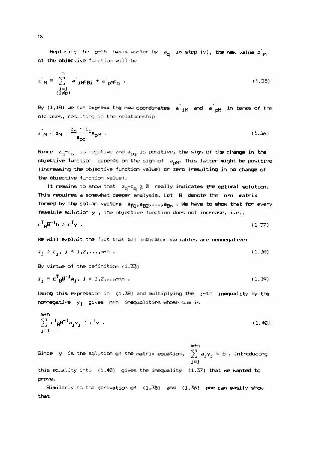
Replacing the p-th basis vector by aq in step (v), the new value z

of the objective function will be

(1.35)

By (1.18) we can express the new coordinates a iM and a pM in terms of the

old ones, resulting in the relationship

Since z9-cq is negative and aw is positive, the sign of the change in the

objective function

(increasing the objective function value) or zero (resulting in no change of

the objective function value).

depends on the sign of am. This latter might be positive

It remains to show that z -c > 0 really indicates the optimal solution. q 9 -

This requires a -hat deeper analysis. Let B denote the nrh matrix

formed by the c o l m vectors

feasible solution y , the objective function does not increase, i.e.,

cTBB-'b 2 cTy . (1.37)

agl,agZ, ..., a& . We have to show that for every

We will exploit the fact that all indicator variables are nonnegative:

zj 2 cj, j = 1,2 ,..., m+n . & virtue of the definition (1.33)

z . J = cTg- laj, j = 1,2, ... m+n .

(1.38)

(1.39)

Using this expression in (1.38) and multiplying t h e j-th inequality by the

nonnegative y, gives m+n inequalities whose sum is

(1.40)

m+n 7-l

Since y is the solution of the matrix equation, 2, ajyj = b . Introducing

this equality into (1.40) gives the inequality (1.37) that we wanted to

prove.

j =1

Similarly to the derivatim of (1.35) and (1.36) one can easily show

that

19

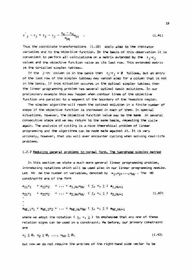
(1.41)

Thus the coordinate transformations (1.18) apply also to the indicator

variables and to the objective function. Ch the basis of this observation it is

convenient to perform all calculations on a matrix extended by the

values and the objective function value as its last row. This extended matrix

is the so-called simplex tableau.

z j i j

If the j-th column is in the basis then zjij = 0 follows, but an entry

of the last row of the simplex tableau may vanish also for a column that is not

in the basis. If this situation occures in the optimal simplex tableau then

the linear programming problem has several optimal basic solutions. In our

preliminary example this may happen when contour lines of the objective

function are parallel to a segment of the kxlndary of the feasible region.

The simplex algorith will reach the optimal solution in a finite number of

steps if the objective function is increased in each of them. In special

situations, however, the objective function value may be the same in several

consecutive steps and we may return to the same basis, repeating the cycle

again. The analysis of cycling is a nice theoretical problem of linear

programming and the algorithms can be made safe against it. It is very unlikely, however, that you will ever encounter cycling when solving real-life

problems.

1.2.2 Reducinq qeneral problems to normal form. The twO-DhaSe simplex method

In this section we state a rmch more general linear programming problem,

introducing notations which will be used also in our linear programming module.

Let W be the number of variables, denoted by x1,x2, ..., xw . The N constraints are of the form

where we adopt the notation < relation signs can be used in

are

xi 2 0, x2 2 0 , ..., xI\N 2 0 ,

but now we do not require the

- <, =, 2 1 to emphasise that any one of these a constraint. As before, our primary constraint

(1.43)

entries of the right-hand side vector to be

nonnegative. The problem is either to maximize or minimize the objective

function

CIlL3X-r ClXl + c2x2 + ... + c w x w --> < . J’ . min

(1.44)

This generalized problem can easily be translated to the normal form by the

follming tricks.

If the right-hand side is negative, multiply the constraint by (-1).

As discussed, a constraint with < is transformed into an equality by

adding a (nonnegative) slack variable to its left-hand side. The same can be

done in an inequality with 2 , this time by substracting a (nonnegative) slack variable from its left-hand side.

The problem of locating the m i n i m is translated to the normal

(maximization) problem by changing the sign of the objective function

coefficients.

With inequality constraints of the form only, the colurms corresponding

to the slack variables can be used as a starting basis. This does not work for

the generalized problem, and we must proceed in two phases.

In the first phase we invent futher variables to create an identity matrix

within the coefficient matrix CI. We need, say, r of these, called artificial

variables and denoted by

variable is added to the left-hand side of each constraint with the sign = or

L , P basic solution of this extended matrix equation will be a basic solution

of the original equations if and only if

such a solution by applying the simplex algorithm itself. For this purpose

replace the original objective function by zI = - E si, which is then

maximized. This can obviwsly be done by the simplex algorithm described in the

previous section. The auxiliary linear programing problem of the first phase

always has optimal solutim where either zI < 0 or zI = 0 . With zI < 0 we are unable to eliminate all the artificial variables and the original

problem has no feasible solution. With

situations. If zI = 0 and there are no artificial variables among the basic

variables, then we have a feasible basic solution of the original problem. It

may h a p p , hanPver, that ZI = 0 but there is an artificial variable among

the basic variables, obviously with zero value. If there is at least one

nonzero entry in the corresponding rcw of the tableau then we can use it as a

pivot to replace the artificial vector still in the basis. If all entries are

zero in the correspmding row, we can simply drop it, since the constraint is

..., sr . Exactly one non-negative artificial

51 = s2 =...= sr = 0 . We try to find

r

i=l

zI = 0 there may be two different

21

then a linear combination of the others.

After completing the first phase we have a feasible basic solution. The

second phase is nothing else but the simplex method applied to the normal form.

The follcwing module strictly follows the algorithmic steps described.

Proqram module M11

ll0E REfl t t t t t t l t t t l t t t l t l t t l t t t l t t t l t t t t t l t l l l t l l t l l l l l l l l t 1182 RE! t LINEAR PROGRAMHING t 1104 REN I TWO-PHASE SINFLEY tlETHOD t 1106 REH t t t t t l t t ~ t ! t l t t t t t t l k l t l t l l l t t l t t l l t t l l l l l l k l l t 1188 RE1 INPUT: 1110 HEM NV 1112 REH ME 1114 HEN E l Ill5 REN E$(NE) 1118 HEN A ( . , , ] 1120 REN 1122 BEN 1124 REH C I N V ) 1 1 3 RER OUTPUT: 1128 REtl ER 1 1 3 HEM 113: REH 11:4 REtl 1136 REN 1138 R i H N 1140 REN H 1142 REH A(N,N) 1144 REK 1146 HEM

1150 REN 1152 REV

1148 REH

NUNBER OF VARIABLES NUMBER OF CONSTRAINTS PRORLEH TYPE: 'HAX' OR ' H l N ' TYPE OF CONSTRAINTS: 'LE ' , 'EQ' OR ' 6 E ' I N I T I A L SIKPLEX TABLEAU All,. .NE, l . , .NV) CONSTRPINT HATRIX COEFFICIENTS All,. .NE,NVt l ) OBJECT I VE FUNCTION COEFF I C IENTS

STATUS FLAG

CONSTRAINT RIGHT HAND SIDES

I OPTINUH FOUND I NO FEASIBLE SOLUTION 2 NO F I N I T E OPTIHUN 3 ERRONEOUS CHARACTERS I N E I ( . ) OR E I

NUHBER OF ROWS I N F I N A L SIMPLEX TABLEAU, N = N E t l NU1HER OF COLUMNS I N F I N A L SIMPLEX TABLEAU,H=NVtLEtGEt l F I N A L SINPLEX TABLEAU OPTIMUM VALUE OF THE J-TH VARIABLE

A ( b ( I , J ) , t l ) OTHERWISE OPTIMUN OfiJECTIVE FUNCTION VALUE IS E I b ( N , f l )

0 IF A(B,J)=I ,

1154 RE\ NODULE CALLED: ti10 1156 REH ---------- I N I T I A L VALUES 1156 LE.0 : E Q 4 :GE=B : E P = . I I B 0 0 I :EN=EP : H A = l E t 3 B 1160 REH ---------- CHECK INPUT DATd 116: FOR 1.1 T O NE 1164 IF A ( ! , N V t l ) ) = B THEN 1170 1166 IF E l l I ) = ' L E " THEN E I ( I ) - ' G E " :GOTO 1170 1159 I F E $ ( I ) = ' G E " THEN E I I I ) = ' L E " 1170 I F E O ( I ) = " L E " OR E $ l I ) = ' E Q " OR E I I l ) = " G E " THEN 1174 1172 ER.3 : GOT0 1340 1174 E Q = E Q - l E l l I ) = " E Q " ) 1176 L E = L E t ( A : ! = B ) t l E I I I ) ~ " L E " ) t ~ A ~ 0 ) & ( E I ! I ) = " G E ' ) 1176 6E=GEt (P'=0! I i E l ( I )="GEE ! + l R < I ) li E I I I ) = " L E U )

1182 IF E W ' N A X " AND E I O ' Y I N " THEN ER=; : GOT0 1340 1134 t 4 = I V t L E t E P + ? t G E + l :N=NEt l

1188 PRINT 'SOLUTION OF THE ACTUAL PROBLEN REQUIRES DIH Ai';N;',';H;')*

iiae NEXT I

1186 RE/ ________________________________________----------------------

1190 RE;^ ._._____________________________________----------------------

22

F I L L SIEIFLEX TbBLEbU I;?: EEfl _________.

1194 JV=NV :J;I:NVtLEtGE I l ? b FOP I.1 T@ NE lLg3 E = ! E I I I ) : "GE")- iE$I I I = ' L E " 1 !208 M(!,NV+1) : I F R'M THEN 1204 1222 A=-A : FOR J = l TO NV :A(I,J)=-R(I,J) :NEXT J :E=-E !?a4 FOR J z N V t l TO W-1 : d ( I , J ) = $ :hlEYT J :P(! ,&=a im I F E=B THEN izia 1 3 8 1 2 l t !F EJO THEN 1214 1212 J4=JR+1 : b i I , J A ) = l : A ( l , J A ) = I :A(I,B)=JA 1211 NEXT I

PHRSE I 1213 IF E O t G E 4 THEN 1294

1222 FOF: J = l TO I4 1 2 4 I F A ! I , J ! < 4 THEN 1 2 3 0 1226 A ( # , J i = 0 1229 FOR 1.1 TO NE :biW,J)=RIN,J)tA(I,J)t(A(1,0)?NVtlEtGE) :NEXT I 1230 NEXT J 1232 IF R(N,H))=-EP THEN 1266 1234 REM ---------- ---------- CHECK F E R S I P I L I T Y 1236 MI=@ 1233 FOR J = l TO fl-1 1240 IF AIN,J) !HI THEN HI=R!N,J l :JP=J 124? NEYT .1 1244 I F HI20 THEN ER=l : GOT0 1340

1246 MI=MR 1250 FOR 1.1 TO HE 125: I F P ( l , J F l ; = E P THEN 1256 1 2 5 4 1256 NEXT I 1258 G O S N 1000 :Ef=EP+EN

J;i=JV+l : A i l , J V ) = E :iF E>0 THEN G(@,JV)=I :A(I,O!=JU

1216 REH ..__......

I?:@ kEM _.__.._._. _.._...... 7.C '!ALLIES

1246 BE)r _ _ _ _ _ _ _ _ _ _ _ _ _ _ _ _ _ _ _ _ CHANGE B A S I S

IF A(!,Mi!blI,JPl(M! THEN M I = A ( I , M ) / A ( I , J P ) : l P = I

TERI l INRTION COMDITION 1260 BE\ _______.__ ____.__.._

12b2 I F d(N,H)( -EP THEN 1236 1264 PEIl ---------- ---------- E L I M l N B T l O H OF ARTlFlClRL VARIABLES 1266 FOR IP=l TO NE 1269 IF UiIP,@!. -NV+LEtGE THEN 1260 1 2 i 8 FGR JP.1 TO N V t L E t G E 1272 !F APS!B(IP,JP!) ' :=EP THEN GOSiJB 1809 : E P E P t E N :GOTO 1 2 B I 1774 A i l P , J f l = B 1276 NEXT J f l?X klIF,0)=8 : b ( I P , H ) = 0 ma NEXT I P 1782 RE\ ---------- PHASE 7 * _

C E 4 FOE 1.1 TO HV : P ( N , J ! - C ( J ) :NEXT J 1 2 M E = [ E I = " l l N " ! - ( E S ~ " W b X " 1266 N=NV+LE+GE+l 1298 B(E,I4)=0 1292 FOR J:NV*l TO I : A i N , J ) = B :NEXT J 1294 FOP 1.1 TO NE :A( I , I4)=A( I ,H+EQ+GEj :NEXT !

1298 FOR J = 1 TO tl 1308 IF R(@,J!:@ THEN 1706 .. i :@: 1394 FOE I=! T O I E :A(N,J!~A!N,J)+E1AII,JilSIN,AI1,B)) :NEXT 1 1!@6 NEXT J G08 FUF: I = l TO NE : b t N , R i l , 8 l ) = 0 :NEXT I

LIES 127b WE\ _ _ _ _ _ _ _ _ _ _ _ _ _ _ _ _ _ _ _ _ _ ;-C Vf,L

b ( N, 2 ) : - E M [ N J 1

23

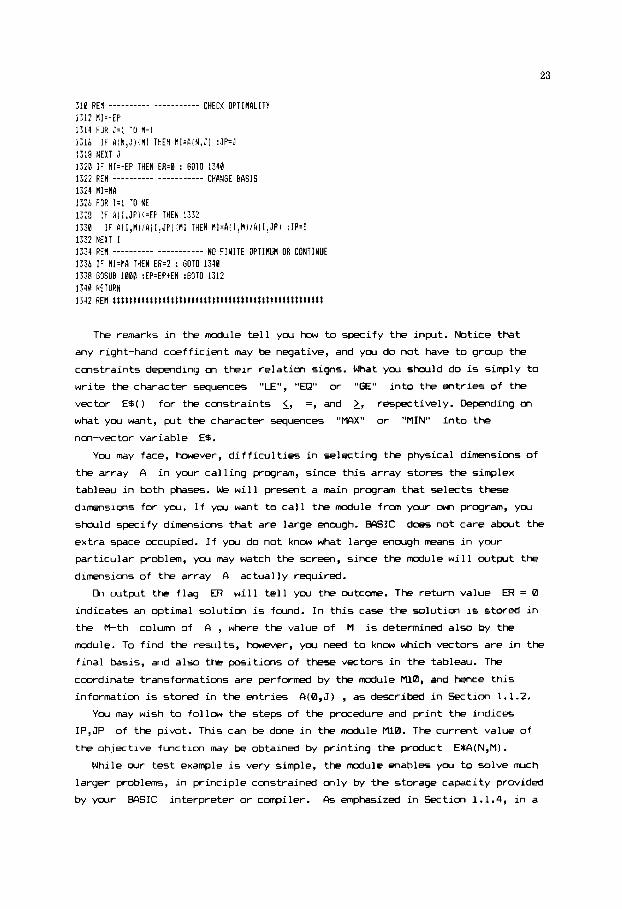
The remarks i n the module t e l l you how to specify the input. Notice that

any right-hand coeff ic ient may be negative, and you do not have to group the

constraints depending on the i r re lat ion signs. What you should do i s simply to

wr i te the character sequences "LE", "EQ" or "GE" i n t o the entr ies of the

vector E30 f o r the constraints <, =, and 2, respectively. Depending on

what you want , plt the character sequences "MFIX" or "MIN" i n t o the

non-vector variable E$.

You may face, however, d i f f i c u l t i e s i n selecting the physical dimensions of

the array A i n your ca l l ing program, since t h i s array stores the simplex

tableau i n both phases. We w i l l present a main program that selects these

dimensions for you. I f y w want to c a l l the module from your own program, you

shwld specify dimensions that are large enough. S I C does not care about the

extra space occupied. I f you do not know what large enough means i n your

particular problem, you may watch the screen, since the module w i l l outplt the

dimensions of the array A actually required.

C h wtpt the f lag ER w i l l t e l l you the outcome. The return value EF4 = 0

indicates an optimal solution i s fcund. In t h i s case the solution i s stored i n

the M-th colunn of A , where the value of M i s determined also by the

module. To f i nd the results, I-asver, you need t o know which vectors are i n the

f i na l basis, and also the positions of these vectors i n the tableau. The

coordinate transformations are performd by the module M10, and hence t h i s

information i s stored i n the entries A(0,J) , as described i n Section 1.1.2.

Y o u may wish to follow the steps of the procedure and p r i n t the indices

IP,JP of the pivot. This can be done i n the module M10. The current value of

the objective function may be obtained by pr int ing the product EXA(N,M).

While our test example i s very simple, the module enables you t o solve rmch

larger problms, i n pr inciple constrained only by the storage capacity provided

by your BFISIC interpreter or compiler. As mphasized i n Section 1.1.4, i n a

24

sequence o f coordinate transformations we accumulate round-off errors. W h e n

selecting a pivot element the test fo r inequality wi th zero actually i s a test

against a small parameter whose value i s increased i n each step t o cmpmsate

the accumulation of errors. Nevertheless, you may encwnter problems wi th

detecting convergence i f there are order of magnitude differences i n the

coeff ic ient m a t r i x . Therefore, i t i s advisable t o perform some scaling o f the

constraints and the variables before solving a larger problem. You may

multiply a l l coeff ic ients and the right-hand side of a constraint by a scaling

factor. Similarly, y w may mult ip ly a l l coeff ic ients i n a colwm of 0 and the

corresponding coeff ic ient in the objective function, but i n th i s case a f te r

solving the problem the corresponding variable must also be mult ip l ied by the

same factor.

Eample 1.2 Solution of the blending problem

Though we solve here only the simple blending problem (1.29-1.30) by

ca l l ing the mcdule M11, we present a main program which, apart f rom the

specific input i n i t s DATA statements, i s rather general and performs a number

of auxi l iary operations. In particular, i t reads the problem, calculates the

dimensions, ca l l s the module, locates and pr in ts wt the results. Later on we

w i l l solve other problems by t h i s program, replacing only the data l ines.

100 REK ____________________-----------------.----------------- 102 REH EX. 1.2. LINEAR PROGRIflnING BY TMO PHRSE SItPLEX IETHOD 104 HEH KERGE 8 1 0 , f l l l

108 HEB [NUHBER OF VARIABLES, NURBER OF CONSTRAINTS) 110 DATA 2,; 112 HEN CONSTRAINTS 114 DATA 6.333333, 0.833333, LEI 50 116 DATA 1.6bbbb7, 'J.166667, LE, 1 6 119 REH OBJECTIVE FUNCTION: !?P DATA 100, 200, MA! 'Xi@ REfl ---------- CHECK DEITA IN@ COflPUTE DIBFNSIONS 3 2 L i z 0 :EQ=@ : G E 4 :READ NV,NE 3 4 FOR 1.1 TO NE 20b FOX J=J TO NV :READ A :NEXT J: READ El,A 208 I F E I= "LE" OR E$='EQu OR E$='GE' THEN 212 ?18 212 I F E$="EOn THEN EQ=E;)+l :GOTO 22: 214 I F EI='GE" THEN 220 ;I6 I F A ' > 4 ldEN L E = L E t l ELSE GE=GE+l 119 G O T 2 ??? 220 I F A:=8 THEN 6 E z 6 E t l ELSE L E z L E t l 2 2 NEXT I 2 4 FOR J=: TO NV :READ I: NEXT :READ El ??b I F ES="#AX" OR E l = " l I l l ' THEN 230 228 LPPlNT "ERROR I# OBJECTIVE FUNCTION SPECIFICATION" : E N @ 324 2;0 t l=NVtL;tEQ+itGEtl : t W E t l ?!: PIN A(#,n),CIN1'),E)INE)

i e 6 RE;^ om

L P P I V T "ERROR I N CONSTRAINT No.":I :GOTO 524

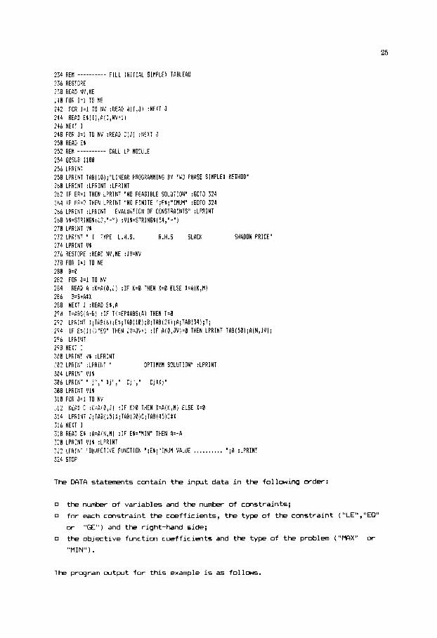
25

:74 PEIl ---------- FILL : N I T I A L SIMPLE! TABLEAU Z h REST3RE

240 FOR 111 TO NE 242 FOR J = l TO N!: :HEAD A ( 1 , J ) :NEYT J 244 READ E ? ( I ! , A ( ! , N V t l ) ?4h N E l T I 246 F I K J = l TO NV :READ C ( J ) :NEXT J 250 READ ES 252 R E 1 ---------- CALL LP MODULE 3 4 605UB 11M 256 LPRINT 258 Li 'KINT TAk(1O);"LINEAR PROGRAMMING BY T l j O F'HASE SINPLEX BETHOD' 260 LFRINT : I F H I N T :LF'RlNT 26: I F E R Z l THEN !PRINT 'NO F E A S I k L E SOLUi!ON" :60TO 3 2 4 ?64 I F ER=? i H E N L P R I N T "NO F I N I T E ";F$;"IBUH" :GOTO 324 :hh LPRINT :LPRINT "EVbLUhTION OF CONSTRAINTS" :LPRINT 268 V l = S T R I N E S ~ 1 2 . ' - " 1 :Vl$:SiRIN6$(54,"- ') 270 L W I N T '!% 272 !Pn'!YT ' I TYPE L.H.S. R.H.S SLACK SHRDOW PRICE" 274 LPRINT V1 276 ?EE;TOHE :REAP NV,NE :JY=NV 278 FOR 1.1 TO NE

28? FOP J = 1 TO NV

?:a REM N V , ~ E

280 B = a

2 8 4 READ a :K=AIB,J! : I F t.=0 THEN x=0 ELSE X = A ( K , M 286 R = k t A t X 2 8 8 NEXT J :READ E%,P ?'il T=ABf(l-6) : I F T i = E P t A B S I R ) THEN T 4 292 LPRINT I;TAB(hj;EI;TRB(lU);B;TbB1?4!;A;TAP(34!;T; ?94 I F E l ( 1 ) : i " E Q " THEN J F J V t l :IF A(0,JV)=B THEN LPRINT T b B ( 5 8 ) ; A ( N , J V ) ; Zob L F F I N T 298 NEXT I :OC L P F I I T V 1 : M I N T 1.02 LPRINT :LFRINT " OPTItlUH SOLUTION" :LPRINT 364 P R I N T SBb LPRINT " J " , " Xj"%' C j " , " C j I X J u 1.08 !PRINT vit

112 HEAP c :K=A!B,J) : I F R > B THEN X=w,ni ELSE 1.8 310 F 3 J=1 TO NV

1.1 4 LPRINT ;:TAB( 1 5 ) 1( ; TAB ( 3 8 !C; T A B ( 4 5 ) C t X Ilh NEhT J S:B HEAD EP :A=kiN,l!) :IF E$="MIN" THEN A = - A 320 LPRINT V1l :LPRINT

3 2 4 STOP z: LPXIIUT "OBJECTIVE FUNCTION ~ ; ~ ~ ; ~ i t i u n VALUE ..,,,,,,,. :LPRINT

The DFYTA s t a t m t s cmta in the i n p l t data i n the following order:

0 the number of variables and the number of constraints;

o for each constraint the coefficients, the type of the constraint ("LE","EQ"

or "GE" ) and the right-hand side;

0 the objective funct im coeff ic ients and the type of the problem ( " M X " or

"MIN" ) .

The program rxltput for t h i s example i s as follows.

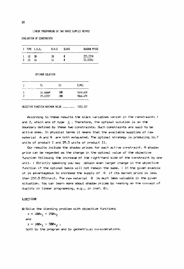
26

LINEAR PROGRRBBING BY TWO PHASE SII(PLE% METHOD

EVALUATION OF CDNSTRkIIlTS

I 16.66664 100 lbbb.664 2 29.:3337 208 5B66.674

________________________________________--------------

OBJECTIVE FUNCTION BAXIfiUB VALUE . . ... . . . ,. 7533.337

k c o r d i n g to t h e s e results the slack v a r i a b l e s van i sh i n the c o n s t r a i n t s 1

and 2 , which are of type 5 . Therefore , the optimal s o l u t i o n is on the

boundary de f ined by these two c o n s t r a i n t s . Such c o n s t r a i n t s are s a i d to be

a c t i v e ones. In physical terms it means that the a v a i l a b l e s u p p l i e s of r a w

ma te r i a l A and B are both exhausted. The optimal s t r a t e g y is producing 16.7

u n i t s of product I and 29.3 u n i t s of product 11.

Our r e s u l t s i n c l u d e the shadow p r i c e s f o r each a c t i v e c o n s t r a i n t . A shadow

p r i c e can be regarded as the change i n the opt imal v a l u e of the o b j e c t i v e

func t ion fol lowing the i n c r e a s e of the right-hand s i d e of the c o n s t r a i n t by me

u n i t . ( S t r i c t l y speaking you may o b t a i n even l a r g e r change i n t he o b j e c t i v e

func t ion i f t h e opt imal basis w i l l n o t r m i n the same. ) In t h e given example

it is advantageous to i n c r e a s e t h e supply of A i f its market p r i c e is less

than 233.3 ECU/unit. The r a w material B is n-uch less v a l u a b l e i n t h e g iven

s i t u a t i o n . Y c u can l e a r n mre a b x t shadow p r i c e s by r ead ing on the concept of

d u a l i t y i n l i n e a r programming, e . g . , i n ( r e f . 8).

E x e r c i s e

So lve t h e blending problem wi th o b j e c t i v e f u n c t i o n s

2 = l m x l + 250x2

2 = l m x , + m x 2 , and

both by the program and by g-trical c m s i d e r a t i m s .

2 1

5 3 -1 0 XI

-3 3 -3 5 x 3

0 6 -2 3 ~4

2 0 4 1

1.3 LU DEKWOSITION

11

x 2 = 1 -2

9

In this section we restrict considerations to an n M nonsingular matrix

A . As show, in Section 1.1, the Gauss-Jordan elimination translates A into

the identity matrix I . Selecting off-diagonal pivots we interchange ~ i ~ m e r w

of I , and obtain a permutation matrix P instead, with exactly one el-t 1

in each row and in each colunn, all the other entries beeing zero. Matrix P

is called permutation matrix, since the operation PCI will interchange saw

ra*h of A . We can save scme efforts reducing A into a triangular matrix and not all

the way to the identity matrix. More generally, we will write

w=LlJ, (1.45)

A as

r 5 3 -1 0

0 -1.2 4.4 1.0

0 4.0 -3.6 5.0

0 6.0 -2.0 3.0 _.

where P is a permutation matrix, L is a lower triangular (has elements only

in the diagonal and below), U is upper triangular (has elements on ly on the

diagonal and above), and [L]ii = 1 . The decomposition will be performed by Gaussian elimination. This classical

method can easily be understood by solving an example.

- 1 x1 x 2 = -3.4

x3 4.61

9.0 _x4.

1.3.1 Gaussian eliminatim

We solve the matrix equation (ref. 9 )

(1.46)

by reducing its coefficient matrix to an upper triangular one. Therefore, let

us first eliminate x1

equatation by factors (2/5) and (-3/5) , respectively, and then substracting from equations 2 and 3 . The resulting equation is

fran equations 2 and 3, multiplying the first

(1.47)

The pivot (i.e., the elemmt we divide by) in this step was 5 , and the factors (215, -315, 0) = (0.4, -0.6, 0 ) are called multipliers. We perform

partial pivoting (see Section 1.1.4) and pick [A14,2 = 6.0 as the next pivot

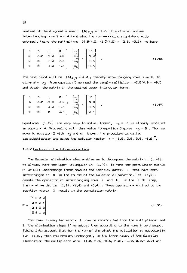
instead of the diagonal element

interchanging rows 2 and 4 (and also the corresponding right-hand side

entries). Using the multipliers (4.W6.0, -1.W6.0) = (0.8, -0.2) we have

CA12,2 = -1.2. This choice implies

x1

X Z

x4-

xs

5 3 -1

0 6.0 -2.0

0 0 -2.0 ::: j 0 0 4.0 1.6

11

= 9-0 . -2.6

-1.6

5 3 - 1 0

0 6.0 -2.0 3.0

0 0 4.0 1.6

0 0 0 3.4 -

(1.48)

9.0

-1.6

-3.4

= .

-x4

The next pivot will be

eliminate x3 from equation 3 we need the single multiplier -2.0/4.0 = -0.5,

and obtain the matrix in the desired upper triangular form:

CAI4,3 = 4.0 , thereby interchanging rows 3 an 4. To

(1.49)

Equations (1.49) are very easy to solve. Indeed, x4 = -1 is already isolated

in equation 4. Proceeding with this value to equation 3 gives x3 = 0 . Then w e

mve to equation 2 with

backsubstitution and gives the solution vector

x3 and x4 k n w . The procedure is called

x = (1.0, 2.0, 0.0, -l.O)T.

1.3.2 Performinq the LU decomposition

The Gaussian elimination also enables us to decompose the matrix in (1.46).

We already have the upper triangular in

P we will interchange those rows of the identity matrix I that have been

interchanged in A in the course of the Gaussian elimination. Let (i,ki)

denote the operation of interchanging row5 i and ki in the i-th step,

then what w e did is (l,l), (2,4) and (3,4) . These operations applied to the identity matrix I result in the permutation matrix

(1.49). To form the permutation matrix

1 0 0 0

0 0 0 1

0 1 0 0

0 0 1 0

P = (1.50)

The lower triangular matrix L can be constructed from the rrultipliers used

in the elimination steps if we adjust them according to the rows interchanged.

Taking into account that for the row of the pivot the multiplier is necessarily

1.0 (i.e., this row remains unchanged), in the three steps of the Gaussian

elemination the multipliers were (1.0, 0.4, -0.6, 0.0), (1.0, 0.8,- 0.2) and

29

(1.0, -0.8). In the second elimination step we performed the interchange (2,4),

and hence write the previous multipliers in the order (1.0, 0.0, -0.6, 0.4).

In step 3 the interchange was (3,4), which will affect all the previous

multipliers, resulting in (1.0, 0.0, 0.4, -0.6) and (1.0, -0.2, 0.8), whereas

(1.0,-0.5), used in this last step, remains unchanged. We put these vectors

into the lower triangular of a matrix and obtain

L.1 0.4 -0.2 1 0 1 . 0 (1.51)

L-0.6 0.8 -0.5 11

It can be readily verified that the matrices (1.461, (1.49), (1.50) and

(1.51) satisfy the relation (1.45). Since L is constructed from nultipliers,

on the basis of the Gaussian elimination algorithn you will understand why the

method works.

Ncw we present a module for the LU decomposition and apply it to compute the

determinant of A . ph is well k n m , det(A) is a number, defined by (1.52)

where the indices

each column of A in each term of the sum, and we add all the possible

combinations. Therefore, the number of term in (1.52) is n! . In each term the indices ki take the values 1,2, ..., n in different orders. Finally, h

in (1.52) is the number of pairwise permutations required to bring all

indices ki into the order l,Z, ..., n .

ki are selected so that there is exactly one element from

Since det(A) = 0 if and only if A is singular, it provides a convenient

way of checking singularity. Determinants have traditionally been used also for

solving matrix equations (ref. 101, but both the Gauss-Jordan method and the

Gaussian elimination are much more efficient. The determinant itself can easily

be calculated by LU decomposition. For the decomposed matrix (1.451

1

det(A) = ------ det(L) det(U) . det (P)

(1.53)

For a triangular matrix the only nmzero term in (1.52) is the product of the

diagonal elements. Therefore, det(L) = 1, and det(U) = . T I [aii . There is

also only a single nonzero entry in det(P) , so that det(P) = +1. Since

det(1) = 1 , det(P) = +1 if the number of row interchanges translating I

into P is even, and det(P)= -1 if this number is odd.

n

1=1

The following module for LU decomposition of an n% matrix A is based m

the algorithm in (ref. 1).

Prcqram module M14

Since only n-1 elimination steps are required for the decanpusiticn, it can

be performed also for matrices with rank(&) = n-1. For simplicity, however,

the module will return the flag ER with value 1 if A is singular.

The decomposition is "in place", i.e., all results are stored in the

lmxtims that matrix A used to occupy. The upper triangular matrix U will

replace the diagcnal elements of A and the ones above, whereas L is stored

in the part below the diagonal, the unit elemmts of its diagonal being not

stored. We will then say that the matrices are in "packed" form. The

permutation matrix P is not stored at all. As discussed, the row interchanges

can be described by n-1 pairs (i,ki), and all information is contained in a

permutation vector kl, k2, ..., kn-l that will occupy the mtries

A ( 1 , 0 ) , A (2 ,0 ) ,..., A(N-1,0) . T h e module writes +1 or -1 into A(0 ,0 )

depending on the number of row interchanges.

31

Example 1.3.2 Determinant of a matrix by LU decomposition

The follwing program performs LU decomposition of the matrix in (1.46) and

calculates its determinant.

N

1 4 The determinant is cwnputed by det(f4) = TI A(1,I) , where cI(0,0) affects

only the sign. The resulting matrix is printed a5 stored, in a packed form. It

it is easy t o recqnise U . The elements of L are stored with opposite

signs, and in the order they originally appeared in the Gaussian elimination.

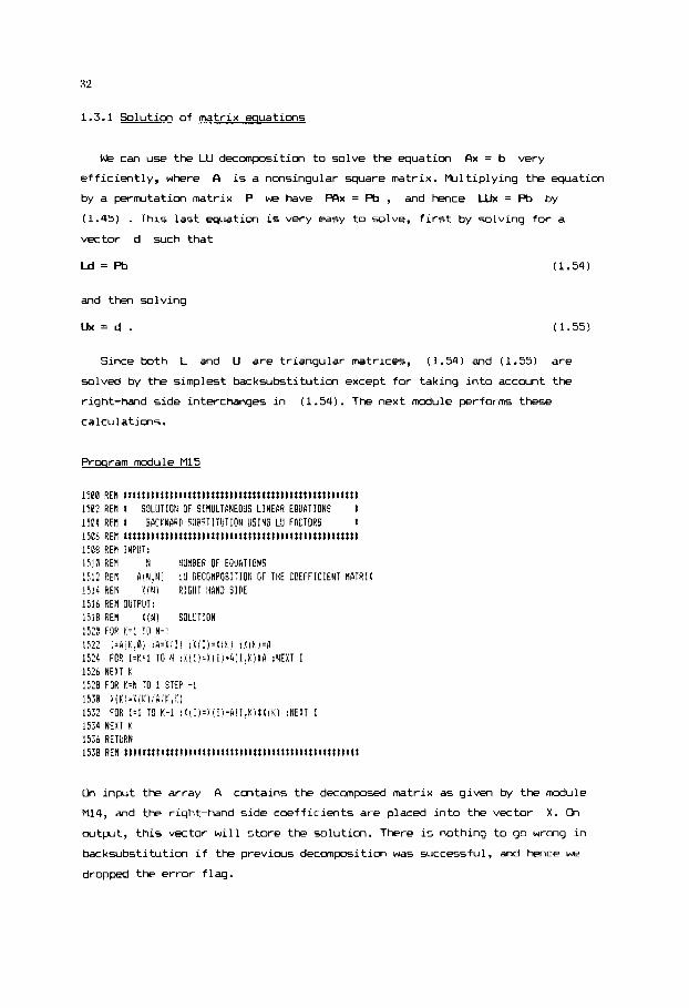
32

1.3.1 Solution of matrix equations

We can use the LU decomposition to solve the equation clx = b very

efficiently, where cl is a nonsingular square matrix. Multiplying the equation

by a permutation matrix P we have PCIx = pb , and hence WX = pb by

(1.45) . This last equation is very easy to solve, first by solving for a vector d such that

Ld=pb (1.54)

and then solving

U x = d . (1.55)

Since both L and U are triangular matrices, (1.54) and (1.55) are

solved by the simplest backsubstitution except for taking into account the

right-hand side interchanges in (1.54). The next d u l e performs these

calcul at ions .

Proqram rodule M15

On inplt the array FI contains the decomposed matrix as given by the module

M14, and the right-hand side coefficients are placed into the vector X . (Ih

wtput, this vector will store the solution. There is nothing to go wrong in

backsubstitution if the previws decomposition was successful, and hence we

dropped the error flag.

33

Example 1.3.3 Solution of simultaneous linear equations by LU decomposition

We u5e the follwing main program to salve (1.46) by the modules M14 and

M15:

100 RE\ ________________..-_____________________-------------------

10; RE( EX. I . ? , ? . SOLUTIO!i OF L I N E A R EQUGTIONS BY LU D E C O B P O S I T I O N 1C4 RE\ RERGE rl l4,\15

108 % E l l ( l U # E R OF EQUATIONS) : ; c DkT4 4 !12 EATU 5 , 13-lq B. 2 % I! 114 0816 2! 5, 4, !, =, 1 l l b D A T A -3 , 5, = I -2 113 DATA 0 , b , - 2 , I , 9 L , , D DFTR 2C: R E X N X4 31!4 A!W.N!,X!N) ?0t FOR 1.1 T O N 263 FOF' J = 1 TO N :REPD A [ I ! J ) :HEIT J 210 READ M q Y ( I j 212 NEXT I 1 1 4 q ~ \ _ _ _ _ _ _ _ _ _ _ c 216 GOSUB 1400 218 I F EY.1 THEN L P R I t i T "CCIEFFIC IENT MATRIX IS SINGULAR" : 6 0 T 3 238

2:: EOSLA 15C0 224 L F R I H T "SirLUTION CF THE SY'STEN CIF L I N E A R EQUATIONS" :LPRINT 226 ?'b=5TFtIIX$( I & , " - " ) 226 LFKINT :;o LPH!#T " I X(I)" :32 LPRINT VB 234 F3R I = l TU ti : L P H I I T USING " X X HU,##I l#": I,X(I) :NEXT 1 ?3t LPRIWT VS : L f F ' I # T K E STOF

REH _ _ _ _ _ _ _ _ _ _ DATA

F E Y _ _ _ _ _ _ _ _ _ _ PEA

ALL DECOIIPOSITIOM MODULE ..I .

LL SOLUTICIN MODULE 22B FEY _ _ _ _ _ _ _ _ _ _ CA

The coefficients and the right-hand sides are separated by the character

but y w can use any other character sequence as a separator. The resulting

outplt agrees with cur hand calculations:

"="

SOL!IT!ON OF THE SYSTEN OF LIlEPX E Q U A T I O N S

I X ! ! )

A special property of solving a matrix equatim in this way is that the LU

decanposition does not involve the right-hand side vector b , in contrast both to the Gauss-Jordan method and to the Gaussian elimination. This is

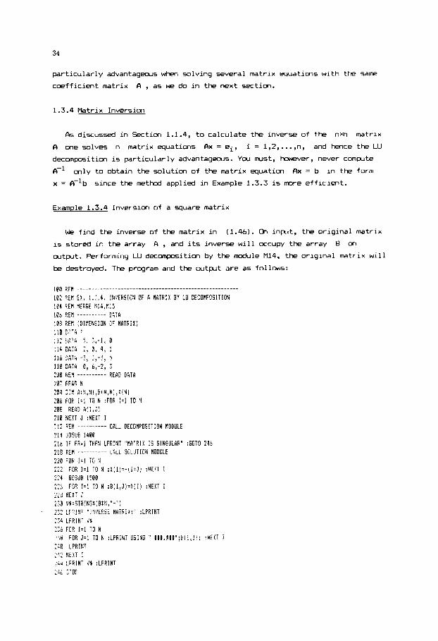
34

particularly advantageous when solving several matrix equations with the same

coefficient matrix A , as we do in the next section.

1.3.4 Matrix Inversion

Fk discussed in Section 1.1.4, to calculate the inverse of the n m matrix

A one solves n matrix equations Ax = ei, i = l,Z, ..., n, and hence the LU

decomposition is particularly advantageous. Y o u must, haever, never compute

A-' Ax = b in the form

x = A-lb

only to obtain the solution of the matrix equation

since the method applied in Example 1.3.3 is m r e efficient.

Example 1.3.4 Inversion of a square matrix

We find the inverse of the matrix in (1.46). Ih input, the original matrix

is stored in the array A , and its inverse will occupy the array B on

wtpt. Performing LU decomposition by the module M14, the original matrix will

be destroyed. The program and the cutpt are as follms:

35

0.235 0.044 0.055 -0.162 -8.108 -0.816 -0.18t. 0,514

P.llB P.147 0.294 -8 .206 -0.147 8.191 -0.118 0.132

Y w may find interesting to compare the results with the output in Example

1.1.4.

1.4 INMRSION ff f7 SYMVETRIC POSITIVE DEFINITE MATRIX

As y w learned in the previws sections, LU decomposition with

built-in partial pivoting, followed by backsubstitutim is a good method to

solve the matrix equation Ax = b . You can use, b v e r , considerable simpler

technics if the matrix A has 5 ~ e special structure. In this section we

assume that A is symmetric (i.e., AT = A ) , and positive definite (i.e.,

xT&x > 0 for a11 x # 0 ; you will encounter the expression

in this book, and hence we note that it is called quadratic form.) The problem

considered here is special, but very important. In particular, estimating

parameters in Chapter 3 y w will have to invert matrices of the form A = XTX

many times, where x is an n m matrix. he matrix XTX is clearly

symmetric, and it is positive.definite if the colurms of X are linearly

independent. Indeed, xT(XTX)x = ( X x I T ( X x ) 0 for every x since it is a sum

of squares. Thus (XxIT(Xx) = 0 implies Xx = 0 and also x = 0 if the

columns of X arc linearly independent.

A = HiT

interesting application is to d e c o m m the inverse in the form A-' = Q Q,

where Q is an upper triangular matrix, easily obtainable from H. We will

need such a decomposition when dealing with error-in-variables models

in Chapter 3 . Y o u may find details of the algorithm in (ref. 21, and the

corresponding BFISIC statements in the module M52 of Chapter 3. Here we

provide a module based on Gaussian elimination, for inverting a positive

definite matrix.

x T ~ x many times

P positive definite symmetric matrix A can be decomposed in the form

where H is a lower triangular matrix, by the method of Cholevsky. An

The method (ref. 2) is based on solving the matrix equation y = Ax , where y is not a fixed right-hand side, but a vector of variables y1,y2, ...,yn

with completely "free" values. To Solve the equation for x in terms of y

notice that all # 0 due to positive definiteness of A, since

all = (elITfkl. We can therefore solve the first equation for

x1

xl, and replace

by the resulting expression in the other equatims:

36

(1.56)

where the new coefficients are:

a Ij = -a1j/a11 , ( j = 2, 3, ..., n ) ,

To proceed we have to assume that a # 0. It can be shown that this

follows from the positive definiteness of fA , (see ref. 2). If a 22 # 0 then

w e solve the second equation of (1.56) for x2 in terms of y1,x3, ..., xn, and replace

Since Cl is positive definite, we can perform a l l the elimination steps in

this way and obtain x in terms of y as

x = e y . (1.57)

xz with the resulting expression in all the other equations.

Since y = Clx according to the original equation, B = fA-' follows, thus we

obtain the inverse in place of the original matrix.

Thwgh the procedure appears to be special, you will notice that it is

essentially a Gaussian eliminatim withwt pivoting.

The following d u l e is b a d M the algorithm in (ref. 2). Its concise

structure is due to cyclic renumbering of both grmps of variables, 50 that

always x1 is expressed and always from the first equation.

37

Proqram d u l e Ml6

1120 REH t t t t t l t t t t t t t t t t t t t t t t t ~ t t t t t t t t t l t t l t t t t t t t t t t t t t t I602 REH tINVERSION OF A POSITIVE DEFINITE SVHNETRIC HRTRIlt 1684 REH t l t t t t t t t t t t t t l t t t t t l t t t t t t t l t t t t l t t t t t t t t t t t t l t 1606 REM INPUT: 1608 REM N 1610 REtl A(N,N) 1112 REM I614 REM OUTPUT; 1616 REH EH 1618 REll 16% REH 1622 REM A(N,C) 1624 HE1

DiflEhlSlGN OF MATRIX MRTRIX (ONLY LOWER TRIANGLE IS USED!

STATUS FLRG 0 SUCCESSFUL INVERSION I RATRIX IS NOT POSITIVE DEFINITE

INVERSE MATRIX (INCLUDING THE UPPER TRIINGLE)

1626 FOR K=N TO I STEP -1 1628 IF A(1!1)<=0 THEN ER=I :GOTO 1654 1630 A(B!N)=IIP(!,l) 1632 FOR 122 T O N 1634 8=A(I,l!tRiB,M) I636 1538 1640 NEWT I I642 FGR 1.1 TO N :Q(N~I!=A(0~1) :NEXT I l b 4 4 NEXT K 1646 FOR I l l TO N-1 1648 FOR J=Itl TO N :A(I,J)=A(J,I) :NEXT J 1150 NEXT I lb52 ER.8 :b54 RETURN 1556 F:EM t t t I t t t I t t t $1 1 t t t t t t t I t t t t t t t t t t t t t t t t t t t t t t t t t t t t t

I F I ? K THEN A[O,i-l)=A ELSE R(0!1-I)=-A FOR 522 T O I : P ( l - l ~ ~ - l ) ~ I ~ l ~ J ) t ~ ( l ~ l ) t I ( 0 , J - l ) :NEXT J

Since FI is symmetric, on input it is sufficient to store its corresponding

portion in the lower triangular part of the array A , including the diagonal. The inverse is also symmetric, but on output it will occupy the entire matrix,

since ithis i advantagwus for further use. The zero-th row of array A is

used as a vector of auxiliary variables, so do not store your ow7 data here. If

the matrix is not positive definite, the d u l e will return the flag ER = 1.

As we discussed, for a matrix of the form

general symmetric matrix, however, the return value ER = 1 does not

necessarily imply its singularity, and you can still try to use the modules M14

and M15 in order to invert the matrix.

XTX this implies singularity. For a

Example 1.4 Inversion of a positive definite matrix

Our test problem will involve the Hilbert matrix of order 6, defined by

[Hblij = l/(i + j - 1) , i,j = 1 , 2, ..., 6. (1.58)

Hilbsrt matrices (and obviously their inverses) are positive definite and are

frequently used for testing algebraic procedures (ref. 1). We present a main

program, with the lower triangular of the inverse of H6 in the DATA statemnts.

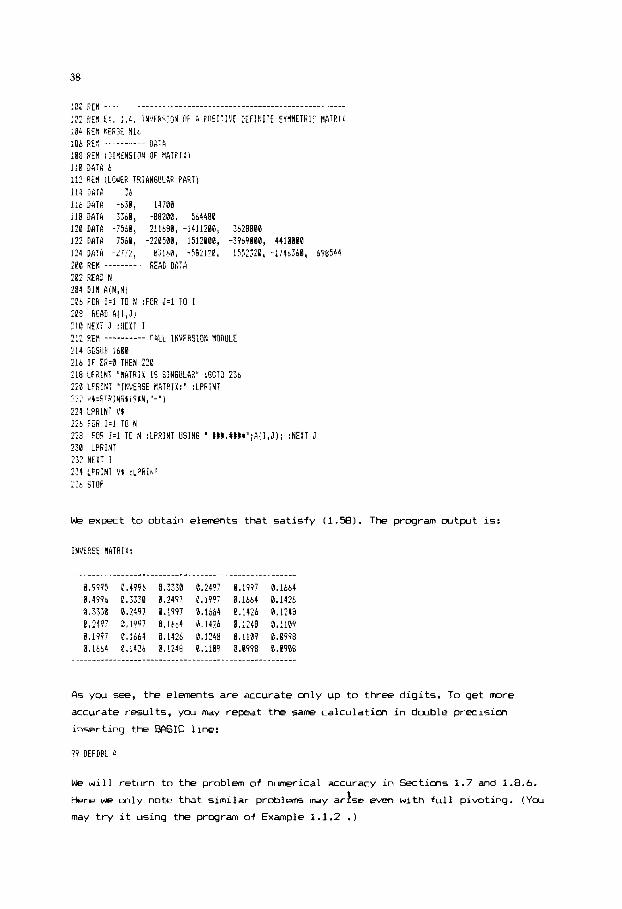
38

We e x p e c t to o b t a i n elwnents that s a t i s f y (1.58). T h e program c u t p u t is:

INVERSE MTSI f :

0s y w 5ee, the elements are accurate m l y up to t h r e e d i g i t s . To g e t mre

a c c u r a t e r e s u l t s , y w may repeat the same c a l c u l a t i m i n doub le p r e c i s l a ,

i n s e r t i n g the BASIC l i ne :

99 DEFDFL 3

We w i l l r e t u r n to the problem of numerical accuracy i n Sectims 1.7 and 1.8.6.

Here w e on ly n o t e that similar problerm may arise even w i t h f u l l p ivo t ing . ( Y w

may t r y i t us ing the program of Example 1.1.2 . )

39

1.5 TRIDIfYXWL SYSTEM OF ECXICITICNS

Another special case of the matrix equation Ax=b is the one with A beeing

tridiagonal, i.e., having nonzero elements only on the diagonal plus or minus

one colunn. For example, the equatims

4x1 + 2 9 = 1 XI + 4x2 + x3 = 2

x2 + 4x3 + x4 = 3 x3 + 4x4 + x5 = 4

2x4 + 4x5 = 5

(1.59)

form a tridiagonal system. To devise a very simple algorithm for solving

equations of this form we need a further special property called diagonal

dminance. The coefficient matrix A is diagonally dominant if

71

laii[ > 1, laij]

large in magnitude. ph in the previous section, tkse assumptions are

restrictive, but satisfied in a number of important applications. For example,

we solve tridiagonal systms of linear equations when interpolating by spline

functions in Section 5.3, and a similar problm arises in modelling

distillation columns (the latter is not treated in this book).

for all i, i.e., each diagonal element is sufficiently

j fi

The Gaussian elimination can be used withaJt pivoting because of diagonal

dominance (ref. 1). Due to the many zeros the algorithm (sometimes called

Thamas algorithm) is very easy to implement:

Prosram module M17

1736 FOR I = N - 1 T O 1 STEP -1 : ~ ~ ~ ~ = ~ K ~ l j - C i l ! t X ( l ~ l ) ) ~ P ~ l l :NEXT I 1755 RETURN

40

The 3 nmzero entries of the i-th row of the coefficient matrix occupy the

variables A(I), B ( I ) and C ( 1 ) ,M that A ( 1 ) and C(N) are not used. We need

an auxiliary vector P O of N elements. Since there i5 no pivoting, you may

experience overflow (i.e., division by a t w small pivot) even for a

nmsingular matrix, if it is not diagonally dominant.

Example 1.5 Solution of a tridiagmal matrix equaticn

The matrix in (1.59) is diagonally dominant, and w e can use module M 1 7 to

mlve the equation. As in example 1.3.3, we separate the coefficients from

the right hand side by the character "=" in each M T A line.

100 RE[ .........._..___._______________________---------------------

102 PEfl Er. 1.5. SOLUTlOli OF L I N E I R EOUMIONS U I T H TRIDIAGONBL #ATHI! 184 RER MERSE HI7

REM ---------- DATA !06 REM (WCtIPEB OF EGURTIONS) !I0 DRTA 5

:!4 DATA !,4!1! =,? : I t DA!A 1!4Q1, = , 3 119 :ATA l i4!! ,=,4

11: D A T A 4,2, = , I

1 3 U A i A : q 3 ! = a 5 ?01 RE! ---------- READ DATA :a2 HER3 I 104 D Ill A I1 ,B(N i ,C( 1; 1 ,D I 10 , X ( k ! , P (ti 1 205 FOP I=! T O N 20E IF 1)1 THEN READ A ( ] ) ?I0 HEAD B(I! 212 IF I < N THE# READ CiI) 214 HERD R$,O(I) 216 Rili 1 TIE REIl ---------- C K L SOLUTION MODULE 2 0 GOSUB 1780 2 2 :PRINT "SOLUTION:" :LPPINT 2 4 V$:STRING$i 15, "-" J 2 5 LF'RI#T " I X(I)n 228 LPHINT v1 2 3 FOE I:! T O H :?PB!NT l ; T M [ b ) ; X [ l ) :NE1T I 3 2 LPRINT V $ :LPRINT 234 STOP

The results are as follow.:

SOLUTIOW:

I XiIi

41

1.6 EIGEWALUES PND EIGENMCTORS ff A R E K SYMTTRIC f " I X

In Section 1.1 we defined the eigenvalue h and the eigmvector u of the

n m matrix A to satisfy the matrix equation

(&XI)U = 0 . (1.m)

This is a homogmwus set of linear equations (i.e., its righ-hand side

zero), and has a ncnzero solution if and only if the c o l m s of (&XI)

linearly dependent. Thus

det(&hI) = 0 ,

is

are

1.61)

which is said to be the characteristic equation of A . a/ the definition (1.52) of the determinant, the left-hand side of (1.61), if expanded, is a

polynomial of degree n in h w h o s e n rwts are the eigenvalues of A . If A is symmetric, all eigmvalues h1,h2, ...,& are real (ref. 10). The i-th

eigenvector ui can be obtained by solving the equation

(&XiI)Ui = 0 . (1.62)

The solutim of this equation is not unique. The eigenvector will be, however,

uniquely defined if we prescribe its length, e.g., by the constraint

I(ui112 = uTiui = 1 , and specify the sign of its first nonzero element. An

eigmvector of unit length is called normalized eigenvector. Assume that all

eigenvalues h1,h2, ..., hn of A are different, i.e., the characteristic

equation has no repeated rwts. Then the eigmvectors

linearly independent and form a basis of the n dimensional space. Furthermore,

the eigenvectors are pairwise orthogonal, and the set

normalized eigenvectors is said to be orthmormal, which mans the property

u1,9, ...,I+, are

u1,9, ...+, of

1 if i=j

0 otherwise. uT.u. = { (1.63)

Consider the matrix B = T-lAT , where T is an n m nmsingular matrix, and

find the eigenvalues of

det(EFh1) = det(T1(AhI)T) = det(A-hI) . (1.64)

B . Since det(T)det(T1) = 1 ,

Thus each eigenvalue of B is an eigenvalue of A and vice versa. I n this

case the matrices A and B are said to be similar and T is called

similarity transformation.

An important application of eigenanalysis is the diagonalization of a

(symmetric) matrix A . Let U dmote the matrix whose columns are the

normalized eigmvectors u l , ~ , ...,I+, . By the definition (1.m) we have

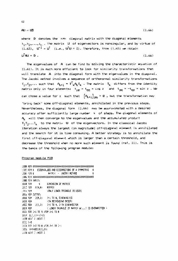
42

w = m (1.66)

where D denotes the nm diagonal matrix with the diagonal elements

X1,x2, ..., hn . The matrix

(1.63), r1 = UT

U of eigenvectors is nonsingular, and by virtue of

(i.e., UTU = I ) . Therefore, from (1.65) w e obtain

UTW = D . (1.66)

The eigenvalues of A can be find by solving the characteristic equation of

(1.61). It is much more efficient to l w k for similarity transformations that

will translate A into the diagonal form with the eigenvalues in the diagonal.

The Jacobi method involves a sequence of orthonormal similarity transformations

T1,T2, ... such that = TTk%Tk . The matrix Tk differs from the identity

matrix only in four elements: tpp = tqq = cos z tW - - -tqp = sin z . We

can chose a value for z such that

"bring back" some off-diagonal elements, annihilated in the previws steps.

Nevertheless, the diagonal form (1.66) may be approximated with a desired

accuracy after sufficiently large number k of steps. The diagonal elements of

% will then converge to the eigenvalues and the accurmlated product

TIT Z...Tk to the matrix U of the eigenvectors. In the classical Jacobi

iteration always the largest (in magnitude) off-diagonal element is annihilated

and the search for it is time consuming. A better strategy is to annihilate the

first off-diagonal element which is larger than a certain threshold, and

decrease the threshold when no m r e such element is fowd (ref. 11). This is

the basis of the following program module:

and

[%+l]w = 0 , but the transformation may

Prcqram m d u l e M1B

18PI REIl t t t t t t t t I t t t t t I t L I I t l t t t I t t t t t I t t I t t t t t t t t t t t t t t t l t :BE? HEN t EIGEMVALUES RND EIGENVECTORS OF R SYRHETRIC t :P04 *Ell t M T R l W - JACOB1 METHOD t !O& REI I l t t t t l t t t l t t t l l t ~ l t t t ~ t t t t t l t t t t t t t t ? t l ~ ~ ~ t t l t t t t t t

lhi2 W N D l f l E N S I O N GF RbTRlX 13i: 7 E l l A!N,W! RATRIX -3!a REIl IBla fiEM W P U T : 1818 PEfl Ulh,J) l=i T O N , EIGENVRLUES l8lE PEl l ! I N DECREASING ORDER) 1922 R E 1 U[l,J) 1.1 TO N , J-TH EIGENVECTDR 1024 HEM i 6 Z FGR ;:I TC N :FOR J.1 TO W 1928 U I I , I j z - ( I z J I

iB3R C E l i J : f t E l T I 1e;; :'=l :9;1 FOE 1=2 TO N :FOR J:! T O I-!

i83B Nil: :NEXT I

RE4 !!PUT:

IONLY LOWER TRIANGLE IS USED)

! LlWER TRIANGLE OF M A T R I X A l , , , ) IS OVERWRITTEN )

ie3t V Z V ~ R B S I A ; I , J ) i

43

la10 IF v.0 THEN 1922 1842 V0=ViNiNl.RBH00S : V 1 4 1844 V=V/h lE46 FOR I@=; TO N :FOR JC.1 TO I@-1 1848 IF ABS(AiIO,JB))<=V THE# 1916 1858 Vl=l 1852 IF A(J@,JQ!=kiI@,l@) THEN 1.1 :GOTO 18t.2

lP56 C:.=ABS(A(J0.J0! - A ( 10, iE1) 1958 'I4zSQHi iR(!0,?0I-A( I!, I01 I'?t4lEii IP,J01*21 !8bB T~2tk(lB,J8)tV?/i!'3tV4i lab! C=l!SER(ltT.'I) i964 S = T t C

l R 6 8 'YS4(IP,iE] 18'0 A ( 10,l@l~Cl1(VS-~tT1A( IB,JB)tTlIR(J0,JB)) IS!? A(J@,~@!=Cll~A(J@,le)r2tTtiliIB,JO)tTlIVS) 1871 RlIC,JB)=@ 1876 FOP J.1 TO JE-1 1878 !8@@ A(J~~J)=CtA(JB,J)tSlb(I0,J) 1682 ic(l0,!)=?'5 1884 N E i T 1 1636 FSR IdBtl TO 10-1

1854 I F AIJB,J0I>A(IS,IVI) THEN W 1 ELSE V2=-1

Cl=C', :sf=S.'? :T!=T"?

V S = - S t A ( J0 , J ) + C I A ( I0,J)

I888 VS=-SIAiI ,JS)tCIII( I 0 , I ) i890 1892 A(IB,I)=VS 1894 NEXT I 18% FOR I=I@+l T O N LE98 1900 NI, JBi=CIA!I, JB)+StA( I! I @ ) 1902 A(Iq10)=V5 1904 NEXT I lY@6 FOR 1 ~ 1 TO N 1908 V S = C t U ( I,IB)-SlU( I ,J0) 1910 UI I,JB)=SIU( I 10l+CtU(I,J0) i912 U(I,IE)=V5 1914 NEXT I 1916 NEXT J @ :NETT I@ 1q18 IF Vl=l THEN V1.C :GOTO 1846 1920 IF V?z'V0 TilEN 1844

A ( 1 ,JPI=CIA( I , J B ) + S t R [ 10, I ]

VS=-Stbi I , J P ) t C t A ( I ,101

T IN DECRERSING ORDER 192-8 PE! _ _ _ _ _ _ _ _ _ _ 1924 FOR Is1 TO N :U(B,I~=G~I,Il :NEXT I 1926 FOR I=? TO N :L= I 1928 IF U(B,L-I))=U(0,L) THEN 1934 1930 19Y IF L!2 THEM L=L-1 :C.OTO 1928 1934 NEXT I 1936 RETURN 1938 RE1 ltttt~ltttttt~tltltt~llllllll!!!llltttttttlltlttllt

FOP 1.0 TO N :14(J,L-l) : U ( J , L - i ) 4 l ( J , L ) :U(J,L)=T :NEXT J

Since the matrix 0 is symmetric, on input we store only its lower triangular

portion (including the diagonal) in the correspmding entries of the array 6.

This matrix will be destroyed during calculations. The resulting eigenvalues

occupy the zeroth row of array U, in decreasing order. The corresponding

eigenvectors are stored in the corresponding colurm of array U. ( Y o u can

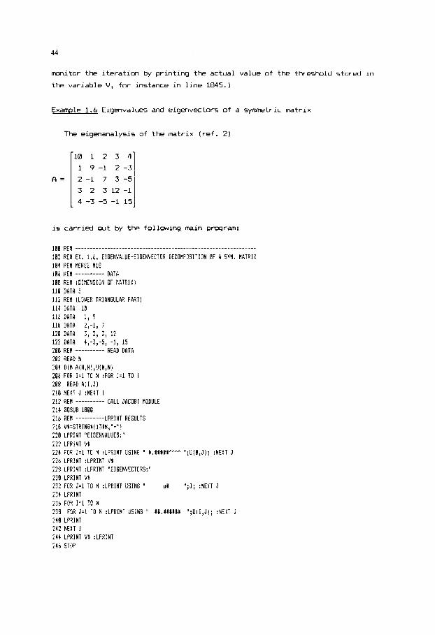
44

A =

m i t o r the iteration by printing the actual value of the threshold stored in

the variable V , for instance in line 1845.)

r10 1 2 3 4

1 9 -1 2 -3

2-1 7 3-5

3 2 3 12 -1

4 -3 -5 -1 15

Example 1.6 Eigenvalues and eigenvectors of a symmetric matrix

The eigenanalysis of the matrix (ref. 2)

is carried cut by the following main program:

100 PEP ________________________________________---------------------- / ,

102 REM EX. 1.t. EIGEN1'ALUE-EiGEWVECTCR DEiOMPOSlTlilN OF 4 SVH. M A T V I X 184 REH bERGE MlB

I05 REM [ D I f l E N S I S N OF W T K I X i 110 DATA 112 RE# I L C I E R TRIANGULAR PART! 114 CIITA 18 115 DATA 1, 9 118 DATA ?,-i, 7 1 3 DATA I?? DATA 4,-3,-5, -1, 15 200 REII ---------- READ DATA 202 READ W 284 DIM A(N,N!,VIN,N! 206 FUR 1.1 TO N :FOR J = l TO 1 208 READ A ( 1 , J ) 210 NEXT J :NEXT I 212 HEM ---------- CALL JACOFI MODULE 214 GOSUB 1800 216 R E 1 ----------LPRINT RESULTS 218 VI:STHING$( 13M, " - * ! 2 0 LPRINT nE16EtiVALUES:n 222 LPRINT 2 4 FOR ;=1 TO N :LPRINT USING " t.X##Wt'" " ;U[$,d j ; :NEXT J 225 L P R l N T :LPRINT 1'1 728 L P R I N T :LPRIIJT "EIGENVECTORS:" 230 L P R I N T It 232 FCH J=l TO N :LPRINT USING " ut " ; J ; :NEXT 1 ?:4 L P R I N T 236 FOR 121 TC N 236 FOR J=1 10 N :LPRINT L E I N G A 1I.XIMXZ " ; U i I , J ! ; : R E U J 240 L P R I N T ?42 NEXT I 244 L P R I N T VO :LPRINT 246 STOP

106 REM _ _ _ _ _ _ _ _ _ _ DATA

:, 2 , 3 , 17

45

The program cutplt is as follaws.

EikEI39ALUES:

Exercise

0 Check the results on the basis of (1.65).

1.7 ACCURACY IN ALGEBRAIC WF.IPUTATIONS. 1LL-WM)ITIOND PROBLEMS

Solving the matrix equation c\x = b by LU decanposition or by Gaussian

elimination you perform a number of operations on the coefficient matrix (and

also on the right-hand side vector in the latter case). The precision in each

step is constrained by the precision of your computer‘s floating-point word

that can deal with numbers within certain range. Thus each operation will

introduce sme round-off error into your results, and you end up with some

residual r = f%i - b # 0 , where 3i is the numerical solution of the equatim.

Y o u have seen that pivoting will decrease the round-off errors and hence the

residual

variables thereby increasing the range of your floating-point arithetics.

r. Y o u can also decrease the errors by using double-precision

bother prwnising way to reduce the residual r is to perform an iterative

improvement of the solution. The equations we use are Ax = b and AZ - b = r.

Substracting the first equation from the secmd one gives I%Z = r , where e = K - x is the error in the solution j i . We have two expressions for r

that yield the equation

since x is the solution we want to improve. We need only to solve this

equation far e and to get the improved soluticn x = Si - e . Of course, neither e can be canpJted without error, but it will certainly reduce the

error in x . We can repeat this step iteratively until all elements of r

cle = f& - b with know terms on the right-hand side,

-

46

will be indistinguishable from zero, which obviously means the machine epsilon

of the computer w e use. I t is highly advisable to calculate at least the

product A% in double precision.

While the residual r can be considerable reduced by iterative improv-t,

in many problems this does not mean that the residual error e will be also

small. To relate e to r , define the norm IlAll of the square matrix A by

IlAXll

IlAll = max ---- - - max IlAxll IlXllW II x 11 =1

I IXI I

(1.67)

which is a straightforward extension of the norm of a vector as defined in

Section 1.1. According to (1.67)

IlAXll 5 l lA l l l lx l l (1.68)

for all A and x . Since r = Fle and FI is nonsingular, e = A - l r , and by (1.68)

llell i I IA -~ I I I I~ I I . (1.69)

Since b = Ax ,

llbll i ll All llxll - (1.70)

Wltiplying the two last inequalities and rearranging, for b f 0 we have

(1.71)

the desired relationship between the relative residual Ilrll/llbll and the

relative error Ilell/llrll , where the llAllIIA-lI1 is called the condition number

of A , denoted by cond(6) . EIy (1.71) cond(A) is the relative error

magnification factor, and its value is at least one. If it is very large, the

relative error in x will be large in spite of carefully reducing the residual

r by m e of the methods discussed. Such problems are said to be

ill-conditioned or nearly singular, and can only be solved by sophisticated

regularization methods (ref. 12). The basic idea of regularization is replacing

A by a sequence of matrices A1, %, ... such that cmd(Ai) <: cond(A) . The matrices Ai approximate A , but we constrain cond(Ai) by a suitable upper

bound. In practice it is far from easy to select a reasonable termination

cmdi tion.

As a numerical analyst you may have to solve inherently ill-conditioned

problems, but in scientific computing there are further opportunities.

Neglecting or coupling unimportant variables, seeking further constraints or

47

devising new experiments fo r fur ther information m y help you t o der ive a

"better" rrcdel and avoid near-singulari ty i n computations. While t h i s i s one of

the basic ideas o f s c i e n t i f i c computing, i t is too genera1 t o be useful, and we

can give you fur ther suggestions only i n par t i cu la r app l i ca t ims (e.g., i n

Chapter 3) .

1.8 APPLICATIWS AND FLRTHER PRDELEMS

1.8.1 Sto ich imet ry o f chemically reactinq species

While l inear algebraic methods are present i n almost every problem, they

also have a number o f d i rec t applications. Che of them is formulating and

solving balance equations f o r extensive quant i t ies such as mass and energy. A

par t i cu la r l y n ice appl icat ion i s stoichianetry o f chemical systems, where you

w i l l discover m o s t o f the the basic concepts of l inear algebra under d i f f e r e n t

names.

We consider a closed system wi th k species denoted by M1, 3, ..., Mk . Let ni denote the quant i ty o f species Mi expressed i n moles. The k-vector

n = (nl, n2, ..., nk)T

change

closed, the mole vector changes 4-i are no t a rb i t ra ry . S t o i c h i m t r y o f fe rs

two ways t o specify the se t o f admissible mole vector changes, i.e. the

s t o i c h i m e t r i c subspace. In par t i cu la r appl icat ions ( e . g . when ca lcu la t ing

chemical equi l ibr ium) one o r the other approach might be more advantageous, so

that w e study t h e i r re la t i on here.

i s ca l led the mole vector and we are interested i n i t s

&I = n - no w i t h respect t o an i n i t i a l s ta te no. Since the sytem i s

The f i r s t approach i s based on e x p l i c i t l y describing chemical reactions. We

wppose tha t there are p reactions taking place i n the system. The j - th

reaction i s described by equation o f the form

(1.72)

where the s t o i c h i m e t r i c coe f f i c ien ts bij are'negatLve f o r reactants (o r so

ca l led left-hand species) and pos i t i ve f o r products (o r right-hand species) o f

the j - t h reaction. The s t o i c h i m e t r i c coe f f i c ien ts can be considered as the

components o f the reaction matrix (o r s t o i c h i m e t r i c m a t r i x ) B of dimension

kxp . I f the system i s closed, any mole vector change i s due t o chemical

reac t ims, i.e.,

C h = B S , (1.73)

48

where the p-vector 5 is formed by the extents of individual reactions.Its

j-th compxlent [&.Ij measures how many moles of "left-hand side" have been

transformed to "right-hand side" in the j-th reactim.

The concept of a closed system can also be introduced without considering

reactions. Chemical species are built from building blocks called atoms. Define

the atom matrix CI , where CAIij is the number of the i-th atom in the

molecule of the j-th species Mj . If the number of different atoms is denoted by a then the atom matrix is of dimension axk . The quantities of atoms in the system can be calculated by summing up their quantities in each

spies, i.e., forming the product Pn. These quantities remain unchanged if

the system is closed, 50 that

& = 0 . (1.74)

For a given system both (1.73) and (1.74) hold, and hence

ABs=0. (1.75)

Since in qn. (1.75) the reaction extent vector 5 can take arbitrary values,

w = o , (1.76)

where 0 is a null matrix of d i m s i m axp . Equatim (1.76) expresses the fundamental relation between the atom matrix

and the reaction matrix of a closed system. The matrices CI and B , however, result in the same stoichiometric wbspace if and only if the wbspace

defined by (1.73) and the one defined by (1.74) are of the same

dimension, in addition to the relation (1.76). We denote the

dimenaim of the stoichiometric wbspace by f also called the stoichiwnetric

number of freedom . If the reaction matrix B is know,, then f = rank(B),

i.e., f is the number of linearly independent reactions. If the atom matrix

CI is k n m , then the stoichiometric number of freedom defined by (1.74) can

be obtained from f = k - rank(CI1, i.e., f is the number of "free" variables

in the general solution of the matrix equation (1.74).

There are the following two basic problems in stoichiometry: -

(i) Given an atom matrix CI construct a (virtual) reaction matrix B

that defines the same stoichiometric subspace and has a minimum number

of colums. -

(ii) Given a reaction matrix B cmstruct a (virtual) atom matrix CI

that defines the same stoichiometric suthpace and has a minirmm number

of rows.

a

49

The solution of problem (i) involves the transformation of the basis. Starting

from the canonical basis w e replace r u n i t vectors by r column vectors of

the m a t r i x A , where r = rank (A) . For notational s impl ic i ty l e t us renumber

the species such that the f i r s t r colums al, 9, ..., + are i n the

resulting basis. Then the table of coordinates takes the form:

ar 0 0 1

where Yr,k_r ccntainr the coordinates of vectors ++I, ..., + i n the

current basis. We select = k - r reactions i n which species Mr+l,

..., Mk are decomposed, respectively, i n t o species M1, f+$, ..., Mr and

obtain the reaction matrix:

Mr+2 ,

- Interchanging the rows of

species.

B y w can easi ly restore the or ig inal order of

To i l l u s t r a t e the above procedure cmsider the species M4, %D, k = 5, and f ix ing the order of CI-$D2, CHD3 and CD4 (ref. 15). Here a = 3,

atoms as C, H and D gives the atom m a t r i x

A = 4 3 2 1 0 . [:: 1 : :] After two transformations we ar r ive a t the table of cmrdinates:

dl 1 314 1/2 1/4 0 a5 0 114 1/2 3/4 1

e3 0 0 0 0 0

50

- From the table r = 2 and f = 5 - 2 = 3 . The (virtual) reaction matrix B

with k = 5 row5 and = f = 3 columns is given by

1 1 - 1 0 0

3/4 1/2 1/4

In m r e familiar chemical terms the following reactions have been

constructed:

Now we turn to problm (ii). Taking the transpose of eqn. (1.76) we obtain

BThT = 0 , (1.78)

where the null matrix 0 is of dimension pXa . It is then foll- from

(1.78) that starting with BT and repeating all the steps needed in problem

(i) we arrive at iT . The number of rows in will be I = k - rank(B) . To see hw the method works, suppose six species M1, b, ..., M6 are know

to take part in the reactions (ref. 15)

The transpose of the reaction matrix is then

0-1 0 0-1 1 , 1 -1-2 1 2 0 0

B T = [ -1 -1 1 2 1 -1

and after two transformations we arrive a t the table of cwrdinates:

b1 b2 b3 b4 b5 b6

b3 -1 -2 1 2 0 0 b6 0 - 1 0 0 - 1 1

e3 0 0 0 0 0 0

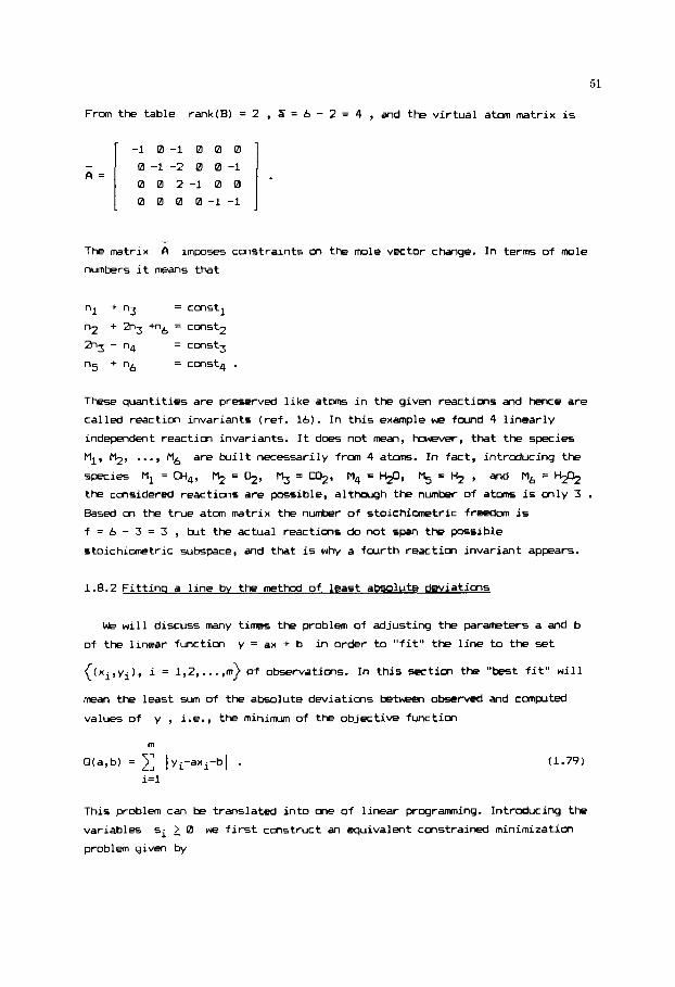
51

- A =

F r a the table rank(B) = 2 , Z = 6 - 2 = 4 , and the virtual atom matrix is

-1 0-1 0 0 0

0 -1 -2 0 0 -1

0 0 2-1 0 0

0 0 0 0 - 1 - 1

- The matrix A imposes constraints m the mole vector change. In terms of mole

numbers it means that

"1 + "3 = cmstl

=3 - "4 = cmst3

"5 + "6 = cmst4 .

n2 + 2n3 " 6 = ccnst2

These quantities are preserved like atoms in the given reactions and hence are

called reaction invariants (ref. 16). In this example we found 4 linearly

independent reaction invariants. It does not mean, however, that the species

MI, %, ..., M6 are built necessarily from 4 atans. In fact, introducing the

species M1 = CH4, 2 = 02, % = q, Mq =v, M5 = 9 , and M6=k$&

the considered reacticns are possible, although the number of atam is only 3 . Based on the true atcm matrix the number of stoichimetric freedan is

f = 6 - 3 = 3 , but the actual reactions do not span the possible

stoichimetric subspace, and that is why a fourth reaction invariant appears.

1.8.2 Fittinq a line bv the method of least absolute deviations

We will discuss many times the problem of adjusting the parameters a and b

of the linear functim y = ax + b in order to "fit" the line to the set

{(xi,yi), i = l,Z, ..., m} of observations. In this sectim the "best fit" will

mean the least sum of the absolute deviations between observed and computed

values of y , i.e., the m i n i m of the objective fwctim

(1.79)

This problem can be translated into m e of linear programning. Introducing the

variables

problem given by si 2 0 we first construct an equivalent constrained minimization

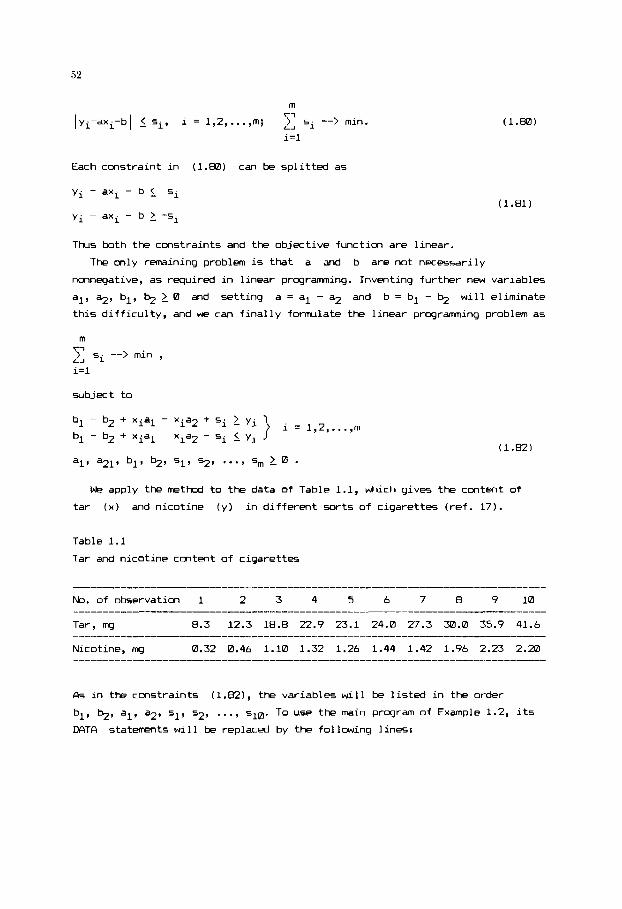
52

m r1

L A lyi-axi-bl 5 si, i = 1,2, ..., m; ) si --> min.

i=l

Each constraint in (1.80) can be splitted as

(1.81)

Thus both the constraints and the objective function are linear.

The only remaining problem is that a and b are not necessarily

nonnegative, as required in linear programing. Inventing further nRnl variables

al, a2, bl, $ 2 0 and setting a = al - a2 and b = bl - b2 will eliminate

this difficulty, and we can finally formulate the linear programming problem as

m

) si --> min , i=l

7-l

L A

subject to

We apply the method to the data of Table 1.1, which gives the content of

tar (x) and nicotine ( y ) in different sorts of cigarettes (ref. 17).

Table 1.1

Tar and nicotine content of cigarettes

No. of observation 1 2 3 4 5 6 7 8 9 1 0

Tar, mg 8.3 12.3 18.8 22.9 23.1 24.0 27.3 30.0 35.9 41.6

Nicotine, mq 0.32 0.46 1.10 1.32 1.26 1.44 1.42 1.96 2.23 2.m

As in the constrainto (1.82), the variables will be listed in the order

bl, $, al, 5 1 9 52, ..., 510. To use the main program of Example 1.2 , it5

IXYTA statements will be replaced by the following lines:

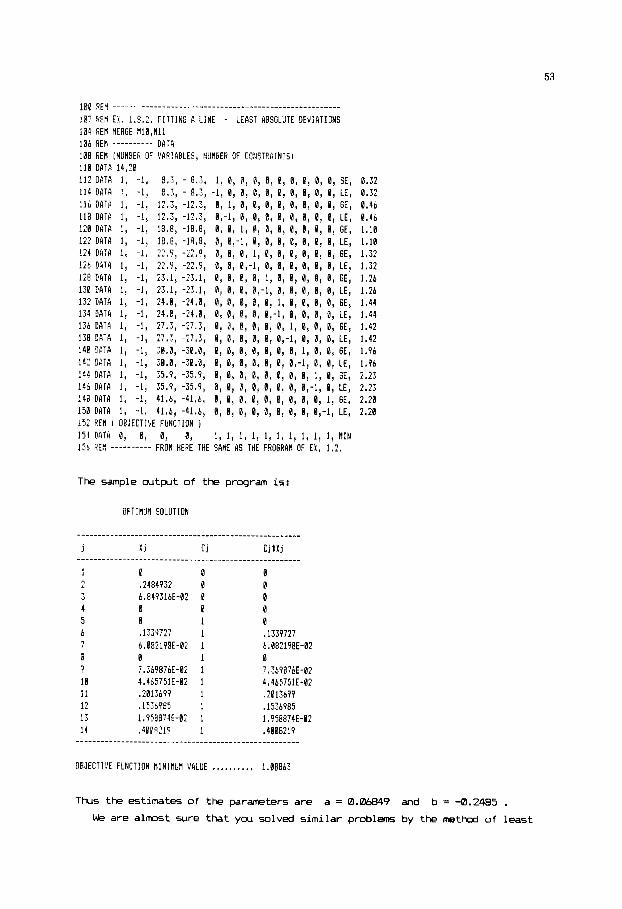
53

100 RE( ..____._________________________________----------.----

la? RE! E l . 1.8.:. F I T T I N G A L I N E - E A S T ABSOLUTE DEVIATIONS 104 RE! I1ER6E fl18,lill

HEN ---------- DATA lh8 REN (kU!UER OF V M I A P L E S , HUNBEH OF CCHSTRAINTS) 110 D A T A 14,Y 112 DBTF i u -1, 8.3, - 8.3, 1, 0, 0, 0, 0, B, 0 , 0, 0, 0, GE, 0.32 114 D A T A 1, - I , 8.3, - 8.3, -1, 0, 0, 1, 0, 0, 0, 0, 0, 0 , LE, 0 . 3 2 116 DATA 1, -1, 1?.3* -12.3, 0, 1, 0, a, 8, 8, 8, 0 , 0 , B, SE, 0.46 118 D A T i 1, -1, 1?,3, - 1 2 , 7 , 0,-1, 8 , 0, 0, 0, 0 , 0, 0, 0 , LE, 0 .46 120 DdTB 1, -1, 18.8, -1R.8, 0, 0, I , 0, 0, 0, 0, 0 , 0 , 0 , SE, 1.18 l?? D A T A 1, -1, 18.8, -18.8, 0, 0,-1, 0 , 0 , 0, 0, 0, 0, 0, LE, 1.10 124 DATP 1, -1, 2 2 . 9 , -22.9, 0, 0, 0 , 1, 8 , 8, 0, 8, 0 , 0, SE, 1.32 12C. DilT4 1, -1, 22.9 , -2.9, 0, 8 , 0,-1, 0 , 0, 0, 8, 0 , 8 , LE, 1.32

130 DATA 1, -1, 23.1 , -23.1, 0, 0, 0 , 0,-1, 0, 0, f l , 0, 0, LE, 1.26 112 DATA 1, -1, 24.0, -24.0, 0, 0, 0, 0, 0, I, 0, 0, 8, 0, GE, 1.44 134 DATA I , -1, ?4.C, -24 .0 , 0, 8, 0, 0, 0,-I, 0, 0, 0, 0, LE, 1.44 136 DATA 1, -1, 27.3, - 2 7 . 3 , 0 , 0, 0, 0, 0, 0, 1, 0, 0, 0, 6E, 1.42 158 DATb I, -1, 2 7 . 5 , -27 .3 , 0, 0, 0, 0, 0, B,-1, 0 , 0, B, LE, 1.42 141 PAT4 1, -1, 3.@, -30.0, 0 , 8, 0, 0 , 0 , 0 , 0 , 1, 8, 0, 6E, 1.96 142 DATA 1, -1, 30.0, -39.8, 0 , 0, 0 , 0, 0, 0 , @,-l, 0, 0 , LE, 1.96 114 DATA 1, -1, TS.?, -35.9, 8 , 0, 0 , 0 , 0, 0, 0 , 0, 1, 0, GE, 2.23 146 D A T A 1, -1, 3 5 . 9 , -3S.9, 0, 0, 0 , 0 , 0, 0 , 0, 0 , - 1 , 0 , LE, 2.23 118 DATA 1, -1, 41.6, -41.6, 0, 0, 0 , 8, 0, 0, 0, 0 , 0, 1 , SE, 2.20 150 D A T A 1, -1, 41.6, -41.6, 0, 0, 0 , 0 , 0 , 0, 0, 0, 0,-1, LE, 2.20 15; HE! [ OBJECTIVE FUt iCTlUN ) 154 D A T A @, 0, B, 0, 1, 1, 1, 1, 1, 1, 1, 1, 1, 1, f l I N 155 RE! ---------- FRO! HEFE THE SARE AS THE PROGRAM OF EK. 1.2.

DATA 1, -1, 23.1, -xi, 0, 0, 0, 0, I , 0, 8, B, 0 , 0, SE, i.?b

The sample o u t p t of the program is:

OPTIHUH SOLUTION

: 2

4 5 b 7 8 7

10 1: 12 11 !4

0 ,2484932 6.RWlbE-02 0 0 .1 ,3V27 6.882199E-02 0 7.3698!bE-02 4 .465 iS lE-02 .201:b91 .15:b98s 1.958874E-fl2 .40082lq

0 0 0 0 0 8 0 0 1 0 1 ,1339727 1 6.08?198E-02 1 0 1 3,369876E-02 1 4 I 465751E-02 1 .?El3699 1 ,153985 1 I .958874E-02 1 .4808?19

________.___________------

ORJECTIL'E FUNCTION MlNl!UH VALUE .,....,.,. 1.08863

Thus the estimates of the parameters are a = 0 . W 9 and b = -0.2485 . We are a l m t sure that you solved simi lar problem by the method of least

54

squares (also k n m as linear regression) and yar know that it is

computationally simpler than the procedure suggested here. The method of least

absolute deviations is, however, more robust, i.e., it is less sensitive to the

errors in observations (ref. 18). We will give you m r e details in Section

3.10.1.

1.8.3 Fittino a line bv the minimax method

Now we solve the previous problem by minimizing the objective function

Q(a,b) = max lyi - axi - bl . ( 1.83)

This procedure is also known as uniform or Chebyshev approximation. We have the

introduce the single auxiliary variable s 0 to translate the minimizatim

of (1.83) into the problem

1 <i <m

Iyi - axi - bl 5 s, i = 1,2, ..., m ; s --> min . (1.84)

Proceeding a5 in the previous section we obtain the linear programing problem

The main program is now used with the DATA statements

174 BATR 120 P4Tb 128 D A T 4

122 DUT4 134 D A T A 1% BPTA 138 D A T R

131 D A T R

, -1, 2?.F, - 2 2 . 4 , -1, LE, 1 , X I -1, 22.1, -2Z,lq 1 , EE, l .?h , -1, 23.1, -23,1, -1, LE, 1 . 3 I -1, :'4.0, -25.0, 1, GE, 1.44 I -1, 24.0* -24.8, -1, LE, 1 .44 I -1, 27.1,-27.T, 1, GE, 1.4; ! -1: ?7.:, - 2 7 . 3 , -1. LE, 1 .42

(1.85)

55

and g i v e s the o u t p l t

I T r P E L.H,S. R.H.5 3 t ; C l i SHADOW P R I C E

.. . i; . l' .- '46 I 4 6

1.1 1.1 1.32 i.:.: 1.26 l.:b

1 , 4 4 1-44 1.4: 1.42 1.9$ 1.96 i 77

" 1- & . ' 1

..-.. ^ * i.'

q q L.'

T h u s a = 0.05939 and b = -0.4601 . In t h i s case the shadow prices are also

of i n t e r e s t and show t h a t p o i n t 8 seems to be an outl ier.

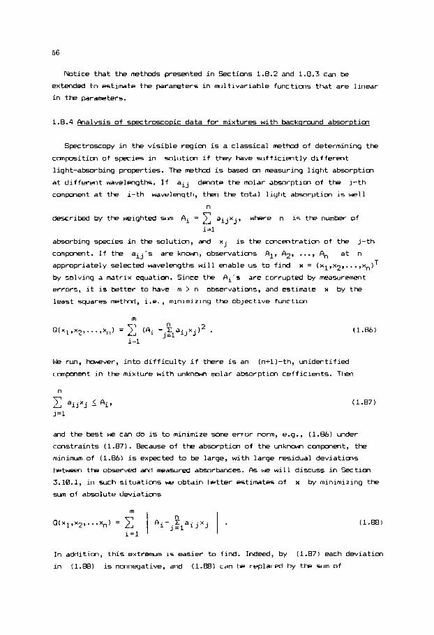
56

Notice that the methods presented in Sections 1.8.2 and 1.8.3 can be

extended to estimate the parameters in mltivariable functions that are linear

in the parameters.

1.8.4 halvsis of spectroscopic data for mixtures with backqrwnd absorption

SpectroKopy in the visible region is a classical method of determining the

composition of species in solution if they have sufficiently different

light-absorbing properties. The method is based on measuring light absorption

at different wavelengths. If aij denote the molar absorption of the j-th

ccmponent at the i-th wavelength, then the total light absorption is well

n

described by the weighted sum Ai = 1 aijxj, where n is the number of

i=l

absorbing species in the solution, and xj i5 the concentration of the j-th

component. If the aij's are known, observations Al, $, ..., An at n

appropriately selected wavelengths will enable us to find

by solving a matrix equation. Since the

errors, it is better to have m > n observations, and estimate x by the

least squares method, i.e., minimizing the objective function

T x = (x1,x2, ..., xn) hi's are corrupted by measurement

m Tl

Q(x1,x2 ,..., xn) = 2, (Ai -.% a. .x.I2 . i=l

1J J

We run, however, into difficulty if there is an (n+l)-th, unidentified

component in the mixture with unknown molar absorption cefficients. T h

(1.87)

and the best we can do is to minimize 5ome error norm, e . g . , (1.86) under

constraints (1.87). Because of the absorption of the unknann component, the

minimum of (1.86) is expected to be large, with large residual deviations

between the observed and measured absorbances. As we will discuss in Section

3.10.1, in such situations we obtain better estimates of x by minimizing the

sum of absolute deviations

In addition, this extremum is easier to find. Indeed, by (1.87) each deviation

in (1.881 is nonnegative, and (1.88) can be replaced by the sum of

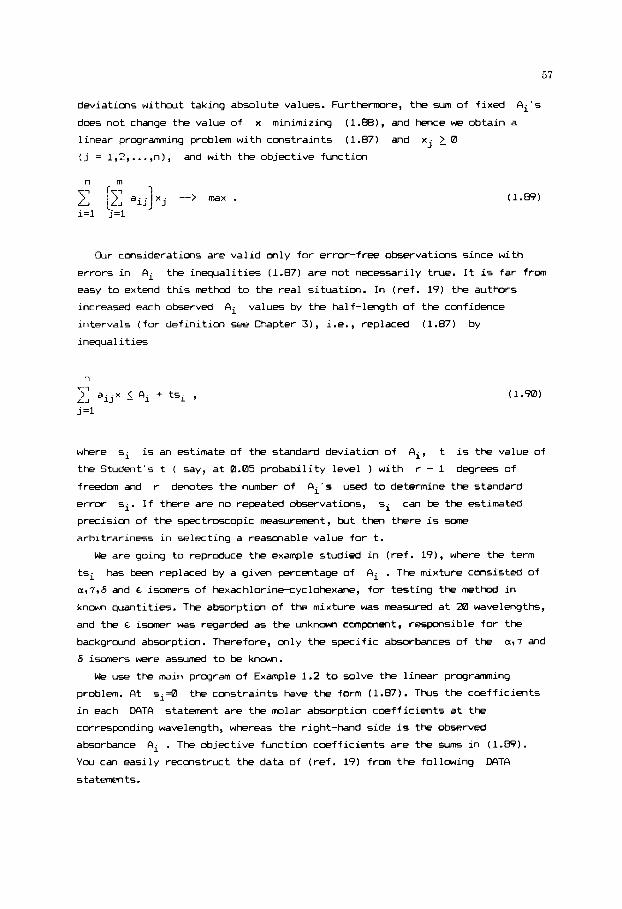
57

deviations w i t h w t taking absolute values. Furthermre, the sum of fixed

does not change the value of x minimizing (1.881, and hence w e obtain a

linear programming problem with constraints (1.87) and x j 2 0

Ai’s

the objective function (j = 1,2 ,..., n ) , and with

Our considerations are va l id only for error-free observations since with

errors i n Ai the inequalit ies (1.87) are not necessarily true. It is f a r f rom

easy to extend th i s method to the real situation. In ( re f . 19) the authors

increased each observed Ai

intervals ( fo r def in i t ion see Chapter 3), i.e., replaced (1.87) by

inequalit ies

values by the half-length of the confidence

n T-1

. L A }

j =1

aijx 2 Ai + tsi ,

where si i s an estimate of the standard deviation of Ai, t i s the value of

the Student’s t ( say, a t 0.05 probabil ity level ) with r - 1 degrees of

freedom and r denotes the number of Ai’s used t o determine the standard

error si. I f there are no repeated observations, si can be the estimated

precision of the spectroscopic measuremeot, but then there i s 5 ~ e

arbitrariness i n selecting a reamable value fo r t.

We are going to reproduce the example studied i n ( re f . 191, where the term

tsi ar7,b and € isomers of hexachlorin=yclohexane, for testing the method i n

known quantities. The absorption of the mixture was measured a t i0 wavelengths,

and the 6 ixxner was regarded as the unknown compent, responsible fo r the

background absorption. Therefore, only the specific absorbances of the a,7 and

6 i m r s were assumed t o be known.

has heen replaced by a given percentage of Ai . The mixture consisted of

We use the main program of Example 1.2 t o solve the l inear programing

problem. A t si=O

i n each statement are the molar absorption coeff ic ients a t the

corresponding wavelength, whereas the right-hand side is the observed

absorbance Ai . The objective function coefficients are the sums i n (1.89).

Y o u can easily reconstruct the data of ( re f . 19) from the following DATA

statements.

the constraints have the form (1.87). Thus the coefficients

DATA

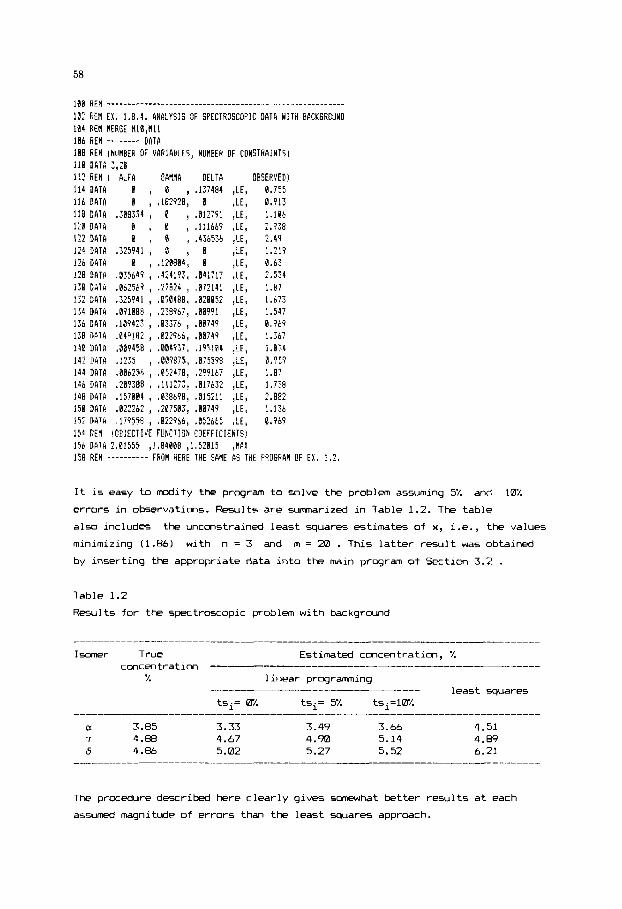
58

I@B REW ________________________________________-----------.--..-

10:' FiEH EX. 1.8.4. ANALYSIS OF SPECTRDSCOF'IC DATA YITH EACPGROUND 104 REM M R G E t!la,Kll 106 KEH -------- DATA 108 KEfl (NUREER OF VAPIARLES, NUMBER OF CONSTRAINTS) 11% DATA Z,X 1 2 RE! [ ALFA B A M A DELTA OBSERVED)

llt DATA 0 , ,182928, I ,LE, 0.913 118 DATA ,388334 , 17 , .i31?!91 ,LE, 1.106 1 3 DATA P , 0 , ,111669 ,I€, 2.938 122 DATR B A , ,436536 , ?El 2.49 12! DATA .i25941 , Ll , B ,LE, 1.219 126 DfiTA 0 , ,121804, B ,LEY 0.63 128 DATP ,83647 , .424i93, .04i717 ,LE, 2.534 138 DATA ,862569 , . ? X 4 , ,072141 , LE, 1.87 11: DATA ,25941 , ,090188, .02605? ,LE, 1.673 134 DdTA .BY1088 , ,238967, ,00971 ,LE, 1.547 135 D A T A ,109423 , .0X76 , ,18749 ,LEI C . 7 8 _. 13 F T 4 .04G!!82 , .0?:965, ,68749 ,LEV 1.367 14B DATA ,089458 I .004937, .19f114 , L E I 1.034 142 TIST4 ,1235 , .0898!5, ,075599 ,LEY 0,959 144 DATA .001256 , ,@524?8, , 3 9 1 6 7 ,LE, 1.8' 145 DATA ,289388 , ,11127?, ,017632 ,LE, 1.738 148 11416 .157084 I ,838698, ,015211 ,LE, 2.88: 158 DATir .0!226? , . N 5 8 3 , ,88749 ,LE, 1.1% IS; Dl)Tfi .17Q558 , ,627956, ,052665 ,LE, 0.969 154 EEi'i !OHJECTIVE FUNCTION COEFFICIE#TS!

114 D A T A e , 8 , . i m a 4 ,LE, e .755

131 D m 2 . ~ 1 5 5 5 , ! , B ~ P P B ,1,5?015 ,MAX 158 REM ---------- FkOM HERE THE M E ii5 THE PROGRAN OF E l . I.?.

It is easy to modify the program t o Solve the problem assuming 5% and 1W.

errors in observations. Results are summarized in Table 1.2. The table

also includes the uncmstrained least squares estimates of x , i.e., the values

minimizing (1.86) with n = 3 and m = 22 . This latter result was obtained by inserting the appropriate data into the main program of Sectim 3.2 .

Table 1.2

Results for the spectroxopic problem with background

I saner True Estimated concentration, X

7. 1 inear programming least squares

tsi= ML tsi= 5% tsi=lO%

a 3.85 3.33 3.49 3.66 4.51 7 4.88 4.67 4.70 5.14 4.69 6 4.86 5.02 5.27 5.52 6.21

The procedure described here clearly gives s-hat better results at each

assumed magnitude of errors than the least squares approach.

59

1.8.5 Canonical form of a Quadratic response function

The conversion y in a chemical reaction was described by the empirical

relationship (ref. 13)

y = 67.711 + 1.944~1 + 0 . 9 0 6 ~ ~ + 1.069~3 - 1.539~~1 - 0.264x22 - - 0 . 6 7 6 ~ ~ ~ - 3 . W x 1 x 2 - 2 . 1 8 8 ~ ~ ~ 3 - 1.212~2~3 (1.91)

as a function of the temperature xl, the feed concentration xz and the

reaction time x3. We want to know whether or not (1.91) has a maximum. More

generally, we are interested in the gwmetric characterization of the quadratic

function

y = a + bTx + xTAx

of n variables x = (x~,x~,...,x~)~, where b is an n-vector and A is an

nW symmetric matrix. From (1.911 in this example we have

(1.92)

-1.539 -1.544 -1.094

-1.544 -0.264 - 0 . 6

-1.094 - 0 . 6 -0.6761

Any extremum point of (1.91) satisfies the

-- * - b + 2 A x = 0 . - ax

6s we will see later, A is nonsingular, hence

equatim

the only solution is

(1.93)

(1.94)

x' = -(1/2)A-'b . It may be a maxinum, a mininum or a saddle point. We can

slightly simplify the problem by setting

into

y - yo = zTAz ,

z = x - xo , wich translates (1.92)

(1.95)

where yo is the value of (1.91) at xo. This point xo i5 the (global)

maxinum point of (1.91) if and only if

matrix A is negative definite. We can easily check this property by

diagonalizing A. Let U denote the matrix formed by the normalized

eigmvectors of

(1.95) is reduced to

Z ' A Z < 0 for all nonzero z , i . e . , the

A . By (1.66), introducing the new variables w = UTz ,

n - yo = -y XiWZi ,

L J

i=l

(1.96)

where Xi is the i-th eigmvalue of A and wi i5 the i-th element of

the vector w , that is wi = uTiz . Expression (1.96) gives the quadratic function (1.91) in its canonical form. This function has maximum at xo if

and only if

eigmvalue-eigmvector decompocition of matrix A by changing the DATA

statements in the program presented for Example 1.6. The following results are

obtained :

xi < 0 for i = 1,2, ..., n. Therefore, we perform the

What can we see f r m these results? The point xo is not a maximum, since the

first eigenvalue is positive. Selecting the canonical variables

w2 = w3 = 0 we can increase the value of y . By orthogonality of the eigmvectors any step x - xo parallel to the first eigenvector u1 results

in wlf 0 and wz = w3 = 0 .

w1 # 0,

To find the point xo m e can use LU decomposition and a backsubstitution.

An other possibility is to apply the results of the eigmvalue-eigenvector

decanpositim directly. By eqn. (1.66)

Y (1.97) ,--1 = m-luT

and hence (1.94) takes the form

x0 = -(1/2)LQ-1UTb . (1.98)

Evaluating this expression is quite easy if taking into account that is a

diagonal matrix with reciprocal values of the eigenvalues in its main diagonal.

We leave to you to compute

higher at the point x = xo + u1 than at the point xo.

D-'

xo and to show that the computed conversion is

1.8.6 Euclidean norm and condition number of a square matrix

In Section 1.7 we emphasized the importance of the condition number ccnd(A),

but did not tell you how to find it. Now w e try to close this gap, first

considering the norm IIAII of a matrix. &cording to (1.67) to find IlAll we

have to maximize the function

l lxl l = 1 . This problem is easy to solve by writing clx in the basis of the

llc1x1I2 = xT(ATAlx subject to the constraint

61

eigenvectors U of ATA, thereby introducing the new variables w = UTx. Since

the columns of U form an orthonormal system, IlwII = IIUTxII = llxll , and by (1.66)

IIAxll~ = WTDW , (1.99)

where D is diagonal matrix with the eigmvalues of ATA in its diagonal. The

function

eigmvector correspmding to the largest eigmvalue Xmx = X1 of ATA, and hence

(1.99) clearly will attain its maxirmm value if w = ul, the

IIAII = ( X m a X P 2 . (l.lrn,

Since ATA is symmetric and positive semidefinite, Xmax is real and

nonnegative. If the matrix is nonsingular (and hence positive definite) then

Xmin f 0 and by (1.97)

IlA-lII = (Xmin)-1/2 ,

where Xmin = An is the smallest eigenvalue of AT& Therefore, by

def inition

cond(6) = ( x ~ ~ / x ~ ~ ~ ) ~ ’ ~ . We note that the values are called the singular values o

(1.101)

its

(1.102)

the matrix - A and they can be determined directly from A , withwt forming AT& . The correspmding numerical method called singular value decomposition is

relatively complex but somewhat m r e accurate then the procedure described

here, for details see (ref. 11).

For exercise find cond(H6) of the Hilbert matrix H6 defined by (1.691.

Give a crude estimate of the relative errors of the columns of H-’6, if the

floating-point numbers are stored to 7 digits.

1.8.7 Linear dependences in data

Observing a process, scientists and engineers frequently record several

variables. For example, (ref. 20) presents concentrations of all species for

the thermal i-rization of a-pinene at different time points. These species

are orpinene (yl), dipentene (yz), all-ocime (y,), pyrmme (yq) and a dimer

product (y5). The data are reproduced in Table 1.3. In (ref. 20) a reaction

scheme has also been proposed to describe the kinetics of the prDcess. Several

years later B o x at al. (ref. 21) tried to estimate the rate coefficients of

this kinetic model by their rmltirespmse estimation procedure that will be

discussed in Section 3.6. They run into difficulty and realized that the data

in Table 1.3 are not independent. There are two kinds of dependencies that may

trouble parameter estimation:

Table 1.3 Concentrations i n the thermal isomerization o f a-Dinene

(1) I f one of the variables is d i f f i c u l t t o measure, the experimenter may

calculate i t s values f rom some known re la t imsh ip , e.g. , a balance

equation . Let Y = [yl,yz,...,yn] denote the m m observation m a t r i x , where

m i s the number o f observations , n i s the number o f variables and y,

is the j - t h column o f the observation matrix. The dependence is o f the

form

n

2; vjyij = c m s t

j=1

( 1.103)

fo r a l l i = 1,2,...,m, where the v j ' s are constant coeff ic ients. The

a f f i n e l inear relat ionship (1.103) can be transformed i n t o a l inear one

by centering the data, i.e., considering the deviat ions xij = yij - y j ,

where y, = [izlyi, ] / m i s the average of the elements i n the j - th

column o f Y . T h the colums o f the centered data m a t r i x X , defined

by [ X I i j = x - ., are l i nea r l y dependent, and hence there ex i s t s an

n-vector u # 0 such that

-

- r m

1,

x u = 0 . (1.104)

M-l l t ip ly ing (1.104) by XT we have ( X T X ) u = 0 , and thus there ex i s t s

an a f f ine l inear dependence of the form (1.103) a m g the columns o f Y

i f and only i f the matrix XTX has a A = 0 eigenvalue. I t i s obv iws

that Amin

raindof f errors.

w i l l equal not zero, but 5ome small number because o f the

63

(ii) The second kind of dependmce is somewhat weaker. In chemical systems the

variables are required to satisfy a number of balance equations, e . g . ,

stoichiometric relations. Therefore, certain affine linear relationships

may exist among the expected values of the responses. In such cases the

least eigmvalue x~~~ of XTX will be larger ttwn in the previous case,

stemming from a linear dependence directly a m g the (centered) data, but

still small.

We need threshold values of Xmin in order to classify the correspmding

linear dependence as (i) or (ii). According to Box at al. (ref. 211, in case

(ii), i.e., a linear dependence in the expected values of the responses

yl, y2, ..., yn, the expected value of the eigenvalue x~~~ can be estimated

bY

~((~,~~)(ii)) = (m-l)uTCxu ,

where u is the corresponding eigmvector of XTX , and C, is the n m

covariance matrix of measurement errors in the observations of y1,y2, ...,yn. In

practice it is usually difficult to find a reliable estimate of

discuss this problem in Chapter 3 ) , and we can get a crude estimate of

E[(Xmin)(ii)I approximating Cx by I?r , where the average variance ”zr is estimated from the residual s u m of squares following a least squares

estimation procedure. These concepts will also be discussed in Chapter 3, and

here we simply state that under the above approximatim

E[(Xmin)(ii)l Z (m - 112,. To obtain a similar upper bwnd on

case (i), when there are only roundoff errors present, Box at al. (ref. 21)

suggested to assume that the rounding error is distributed uniformly with range

-0.5 to +0.5 of the last digit reported in the data. The rwnding error

variance “zre is then givm by the range squared divided by 12, and

E((Xmin)(i)) Z (m-l)”zre . In Table 1.3 the concentration data are reported to the nearest 0.1 percent and therefore the range of the last reported digit is

from -0.05 to +0.05 or 0.1. Thus, for class (i) of the dependences we have

EC(Amin)(i)l 5 71(0.1)2/12 Z 0.006 . As we will show in Section 3.6, the

average variance 2 5 0.6 and hence the threshold for class (ii) is given by EC(Xmin)(i)I Z (m-l)> z 4.2 .

eigmvectors of XTX, where x is the centered observation matrix from the

data of Table 1.3. The program outplt is as follows.

( 1.105)

Cx (we will

-

Xmin(i) in the

-

-

We used the program given in Example 1.6 to calculate the eigmvalues and

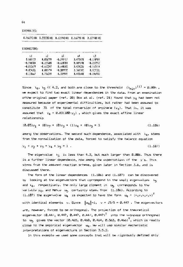
64

Since

we expect t o f ind two exact l inear dependences i n the data. F r m an exemination

ofthe or ig inal paper (ref . 20) Box a t a l . ( ref . 21) fwnd that y4 had been not

measured because of experimental d i f f i c u l t i e s , but rather had been assumed to

constitute

assumed that

relationship

x4, x5 << 4.2, and both are close t o the threshold (Xmin)(i) = 0.006 ,

3% of the to ta l cooversion of a-pinene (y4) . That is, i t was

y4 = 0.03(1Wa-y1) , which gives the exact a f f i ne l inear

(0.@3)~~ + ( 0 ) ~ ~ + ( 0 ) ~ ~ + ( l ) y 4 + ( 0 ) ~ s = 3 (1.106)

among the observations. The second such dependence, associated with

frm the normalization of the data, forced t o sat is fy the balance equation

x4, s t m s

Y 1 + Y 2 + Y 3 + Y 4 + Y 5 = 1 . (1.107)

The eigenvalue X3 i s less than 4.2, but much larger than 0.awb. Thus there

i s a further l inear dependence, now a m g the expectations of the y ' s . This

stems from the assumed reaction scheme, given la te r i n Section 3.6, and i s

discussed there.

The form of the l inear dependences (l.lmb) and (1.107) can be discovered

by looking a t the eigenvectors that correspond to the small eigmvalues

and X4, respectively. The only large el-t i n u5 corresponds t o the

variable y4, and hence u5 certainly stems from (1.10A). According t o

(1.107) the eigenvalue u4 i s expected to have the form u4 = (v,v,v,v,v)

with identical elements v. Since IIu411=1, v = J5/5 = 0.447 . The eigmvectors

are, however, forced to be orthogonal. The projection of the thwre t i ca l

eigenvector (0.447, 0.447, 0.447, 0.447, 0.447IT

to

close to the empirical eigenvector

interpretations of eigenvectors i n Section 3.5.2.

X5

T

i n t o the subspace orthogonal

gives the vector (0.465, 0.468, 0.464, 0.363, 0.466IT, which i s rea l l y u5 u4. We w i l l use s imi lar mechanistic

I n th i s example we used some concepts that w i l l be r i go rws ly defined only

65

in latter chapters. It is, however, difficult to avoid such flaws in structure

when presenting applications of essentially algebraic methods, since the

problems themselves usually c o w from other application areas.

1.8.8 Principal component and factor analysis

We generalize the discussi~ of the previous section by considering the m m

raw data matrix Y, obtained by measuring the variables yl, y2, ..., y, at

m sample points. Depending M the physical meaning of the data we apply sane

kind of preprocessing of the raw data to obtain the observation matrix X

with the same number of row5 and colums, respectively. In the previous section

we considered centering as possible preprocessing. Another useful procedure is

normalizing a colwm by the empirical standard deviation of the observations in

the given column.

decomposition of the n m empirical covariance matrix Cx = XTX (ref. 22-24).

The eigenvalues are denoted by

inequality follows from the presence of sow random error in the data. Using

the eigmvector5 ul, u2, . . . , un, define the new variables

Principal canponent analysis is based a, the eigenvalue-eigenvector

x1 2 x2 2 ... 2 An > 0 , where the last

2, = x-1/2n(ulnxl + U a X 2 + . . . + unnxn)

(1.110)

called principal components or abstract factors. We calculate the row vector

(zl, z 2 , ..., zn) for each sample point, and construct the mm principal

component observation matrix 2 from these row5. By (1.110) 2 is given by

z = xm-1/2 , (1.111)

where D-li2 is the diagonal matrix with the square roots of the reciprocal

eigenvalues in its diagonal. Y w can readily verify that

thus the principal components are uncorrelated and each variable

empirical variance 1. These are the important properties we will exploit.

C, = ZTZ = I , and

zi has the

Since UTU = I, by (1.1W) the observation matrix can be written as

X = ZD1/2UT . (1.112)

Thus the variables x are represented by the linear combinations

(1.113)

of the p r i n c i p a l cmpments. Th i s expres s ion is ve ry in fo rma t ive . Each v a r i a b l e

zi has u n i t va r i ance , and i n c r e a s i n g t h e index i the corresponding p r i n c i p a l

components zi w i l l less and less i n f l u e n c e the observed v a r i a b l e s , according

to the dec reas ing e i g m v a l u e s X i .

P r i n c i p a l components corresponding to small e igenva lues may g i v e e f f e c t s

w i th in the range of measuremmt errors. Having information on the magnitudes of

these errors e n a b l e s u s to c l a s s i f y the p r i n c i p a l components as primary and

secondary ones. T h e s i m p l e s t method of c l a s s i f i c a t i o n is cons ide r ing a

th re sho ld on the e igenva lues , as we d i d i n the p r e v i w s section, bu t there

e x i s t s a l a r g e number of more involved procedures ( r e f . 23). In s m

a p p l i c a t i o n s the selected primary p r i n c i p a l components are r o t a t e d i n o r d e r to

f o r m f a c t o r s which can be better i n t e r p r e t e d i n phys i ca l t e r m s . Sometimes one

wants to know on ly the number of primary f a c t o r s . For example, spec t roscop ic

a n a l y s i s of a number of mix tu res con ta in ing the same components i n d i f f e r e n t

compositions w i l l e n a b l e us to f i n d the number of species w i t h o u t any f u r t h e r

information on their p r o p e r t i e s .

Another important problem is to reproduce the obse rva t ion matr ix us ing on ly

the primary f a c t o r s , i.e., dropping sane small terms i n (1.113) that l i k e l y

stem from measurement error.

Represent ing the d a t a i n terms of a small number of primary f a c t o r s is a

very e f f i c i e n t way of s t o r i n g information. Th i s approach is f r e q u e n t l y used i n

spec t roscop ic l i b r a r i e s , designed to i d e n t i f y unknown species by c m p a r i n g

their spectra with ones f i l e d i n the l i b r a r y .

Y w w i l l better understand the g o a l s of f a c t o r a n a l y s i s cons ide r ing f i r a t

the h igh ly i d e a l i z e d s i t u a t i o n wi th e r r o r - f r e e o b s e r v a t i o n s and on ly r < n

l i n e a r l y independent columns i n the matr ix X . As d i scussed i n Sec t ion 1.1,

a l l columns of X are then i n an r-dimensional subspace, and you can w r i t e

t h e m as l i n e a r combinations of r b a s i s v e c t o r s . S i n c e t h e matr ix X T X h a s

now r nonzero e i g m v a l u e s , there are e x a c t l y r nmvan i sh ing v e c t o r s i n the

m a t r i x 2 def ined by (l.lll), and these v e c t o r s form a b a s l s f o r the subspace.

T h e corresponding p r i n c i p a l cmp-ents zl, z2, ..., zr are the c o o r d i n a t e s i n

t h i s b a s i s . In t h e real l i f e you have measurement errors, the c o l u m s of X

67

are no more linearly dependent, and XTX has n - r -11, but nonzero

eigmvalues. Nevertheless, choosing the primary factors you select the subspace

what is really important, and the primary factors are coordinates in the basis

for this subspace.

Exercise

0 Reproduce the observation matrix in Sectim 1.8.7 using 1, 2, 3, and 4 , respectively, primary factors. Compute the sum of reproduction error squares

for each case. Compare these sums with the following wms: X2 + X3 + h4 + X5,

X3 + X4 + X5, X4 + X5 and X5, respectively.

REFERENCES

1

2

3

4

5

6

7

8 9

10 11

12

13

14

15

16

17

18

G.E. Forsytk and C.B. Moler, Computer Solution of Linear Algebraic Systems, Prmtice Hall, Englewood Cliffs,N.J., 1967. J.H. Wilkinson and C. Reinxh, Handbook for AutoMtic Computation, Vol. 11, Linear Algebra, Springer Verlag, New York, 1971. V.N. Fadeeva, Computational Methods of Linear Cllgebra, Dover Publications, Inc., New York, 1959. A. Ralston and P. Rabinowitz, A First h r s e in hnerical Pnalyais, 2nd ed., PkGraw-Hill, New York, 1978. A. Ralston and H.S. Wilf (Editors) , Mathemtical Methods for Digital Computers, Vol. 1, John Wiley, New York, 1964. J. Stoer and R. Bulirxh, Introduction to I\)_lmerical Fhalysis, Springer Verlaq, New York. 1 W . -. G.B. Dantzig, Linear Programming and Extensions. Princetm Lhiversity Press, 1963. G. Hadley, Linear Programming, AddiMn-Wesley P.C., Reading, Mass., 1963. R.L. Johnston, IU-lmerical Methods, A Software Approach, John Wiley, New York,1982. G. Hadley, Linear Algebra. Addison-Wesley P.C., Reading, Mass., 1961. G.H. Golub and C.F. Van Loan, Matrix Computations, Johns Hopkins Lhiversity Press, Baltimore, 1983. A.N. Tihanov and V. Ya. Arsenin, Solution Methods of Ill-Conditioned Problem, Nauka, Moscow, 1979. (in Russian) N.R. Armndson, Mathematical Methods in Chemical Engineering, Matrices and their Applications, Prentice-Hall, Englewood Cliffs,N.J., 1966. R. Aris, Imtrduction to the Anaysis of Chemical Reactors, Prentice-Hall, Englewood Cliffs,N.J., 1961. W.R. Smith and I. Missen, Chemical Reaction Equilibrium Analysis, John Wiley, New York, 1982. K.V. Waller and P.M. Makila, Chemical reaction invariants and variants and their use in in reactor modeling, simulation and control, Ind. Eng. Chem. Proc. D e s . Dev. 20 (1981) 1-11. 8. Carnahan and J.D. Wilkes, Digital Computing and Mmerical kthcds, John Wiley, New York, 1973. FI. Blwmfield and W. Steiger, Least absolute deviations curve fitting, SIN J. Sci. Stat. Cornput.,

(in Russian).

the liquid phase. J. h r . Chem. Soc. 69 (1947) 319-325.

1 (I=) ~0-301. 19 A.F Vasilyev and M.B. Pankova, Zavodskaya Laboratoriya, 9 (1972) 1076-10B3

20 R.E. Fuguitt and J.E. Hawkins, Rate of thermal isomrization of a-pinme in

68

21 G.P.E. Box, W.G. Hunter, J.F. MacGregor and J. Erjavec, Some problms associated with the analysis of multirespmse data, Technometrics, 15 (1973) 33-51.

Butterworth, London, 1963.

New York, 1m.

A. Dijkstra and L. Kaufman (Editors), Evaluation and Optimization of Laboratory Methods and Analytical Procedures, Elsevier, Wterdam, 1978.

22 D.N. Lawley and A.E. Maxwel l , Factor Analysis a5 a Sta t i s t i ca l Method,

23 E.R. Malinowski and D.G. b r y , Factor Analysis i n Chemistry, John Wiley,

24 S. Wold, Factor and Principal Component Analysis, i n D.L. Massart,

69

Chapter 2

NONLINEAR EQUATIONS AND EXTREMUM PROBLEMS

On the basis o f the p rev iws chapter y w can t e l l i n advance t k number o f

el imination steps or, more generally, the number o f algebraic operations

required fo r solving the system c\x = b of l inear equations. Chfortunately,

there ex i s t no s imi lar f i n i t e procedures f o r solving the system o f nonlinear

equations o f the general form

f ( x ) = 0 . (2.1)

Root f inding i n (2.1) invar iably proceeds by i t e r a t i o n ( re fs . 1-31,

constructing a sequence

t o converge t o a root r o f (2.1). Natural ly you would l i k e t o terminate the

i t e ra t i on when Xk sa t i s f i es the condit ion llxk - rll 5 E , where E i s a

desired error bound, but the rwt r i s unknown. Some pract ical termination

xl, x2, ... of approximate solut ions that are expected

where El and E2 are small parameters, and I M i s an upper bcund on the

number of i terat ions. Neither o f these condit ions w i l l assure that

rea l l y close to the root r , but w i l l save you frm useless i t e r a t i m s that

can move Xk even fur ther apart f r o m r because o f the accumulating rwndo f f

errors. Since y w cer ta in ly know what r e a m a b l e tolerance means f o r your

part icular problem, fol lowing the i t e ra t i ons M the screen i s of ten superior t o

sophisticated convergence c r i t e r i a .

xk i s

Another class o f problems requir ing i t e ra t i on i s minimization or

maximization of a nonlinear scalar valued function g which depends on one or

i n r e variables x ( re f . 4 ) . A value r of the independent variables i s a

local minimum p i n t i f g ( r ) < g (x ) f o r a l l x i n a neighborhccd o f r . Simi lar ly, r i s a local maximum i f g ( r ) 2 g(x) i n a neighborhwd, and then

r i s a l o r a l m in imum point of the function -g(x) . Therefore, we will

r e s t r i c t consideration t o the problem

g ( x ) --> min . (2.2) X

In some problems the possible region o f independent variables i s defined by

equali ty or inequal i ty constraints. As y w have seen i n Section 1.2, such

constrained extrermm problems are easy t o solve i f both the cms t ra in t s and the

70

objective function are linear. In the nonlinear case the most popular approach

is to convert constrained problems into a sequence of unconstrained ones by

penalizing points outside the feasible region (ref. 5 ) . Such sophisticated

methods are beyond the scope of our book. Nevertheless, our programs will also

keep the estimates within a region defined by the user in order to avoid

functim evaluation at points where the function may not be defined at all.

This simple test is sufficient if the extremum is known to be at some inner

point of the feasible region.

While the number of independent variables is arbitrary in cur definitions,

it makes a tremendous difference in cmpltations. Simultanews solution of n

equatims and minimization in n dimensions are much m r e difficult than in

one dimension. The main difference bet- one and several dimsions is that

in one dimension it is possible to "bracket" a root or a local minimum point

between s m bracketing values, and then to tighten the interval of

uncertainty. This gives rise to special algorithms, and hence the solution of a

single equation and minimization in one variable will be dixussed separately

f r m the multidimensional methods.

Solutions of equations and those of extremum problems are closely related. A

point r is the root of the equations f(x) = 0 only if it minimizes the

function

differentiable function g satisfies the equations % ( % ) / a x = 0 . Though a r w t is not necessarily an extremrm point of g, this transformation may be

advantagwus in one dimension. As will be discussed the situation is, however,

completely different with m r e than one variable.

We would like to c b s e methods that are robust, i.e., will converge to a

solution if our initial estimate is reasonably close to it and, in addition,

will cmverge rapidly. Apart from the one-dimensional case, where the snlution

can be bracketed and found in a very safe way, robustness of a method is nuch

problem dependent. To measure hcw fast the convergence is we can use the local

approximation

g = fTf. RI the other hand every local extrmm point of a

in a small neighborhood of the solution

in the k-th iteration. The exponent p depends only on the method, which is

then said to have cmvergmce of order p . Since C is problem dependent and

this analysis is local, the order p does not characterize the cmputational

effort required to solve a particular problem. For this latter plrpose one can

use the number of iterations. We may need, however, to evaluate the function

(and its partial derivatives, if the algorithm requires t h ) different times

in each iteration of different methods, and hence a sanewhat m r e realistic

r , where ek = xk - r is the error

71

measure of the computational e f fo r t i s the number of equivalent function

evaluations.

2.1 MIvII\EAR EWFlTIONS I N auE VARIQELE

2.1.1 Cardano method for cubic equations

The roots of quadratic and cubic equations are w e l l kncm as algebraic

expressions of the equation’s coefficients, and hence t h i s section i s cmlete ly

disconnected f r o m the rest of the chapter. Nevertheless, these simple problems

are so frequently encantered that we cannot ignore the i r special solutions.

Y o u certainly knm hcw to solve a quadratic equation, but we provide a routine

for solving the cubic equation

Ax3 + Ex2 + Cx + D = 0 . (2 .3 )

Since A f 0 (otherwise we have a quadratic equation), introducing the

variable x = y - El(=) , (2.3) can be reduced to the form

Y 3 + PY + 9 = 0 9

where p = (=/A - B2/A2)/3 and q = (Z7D/A - 9BC/A2 + 2$/A3)/27 . 2.4)

We f i r s t evaluate the discriminant

cubic equation has three (but not necessarily d i f ferent ) real roots. I f , M the

other hand, d > 0 , then the equation has me real rmt and a conjugate pair

of complex roots. Since y w f ind the expressions for the roots i n mathematical

tables we proceed to the module.

d = ( ~ 1 3 ) ~ + (q/2I2 . I f d 5 0 , then the

Proqram d u l e IT0

3 0 8 FEN t l t l t t t t t t t t t t t l t t t t t t t t l t l l t t t l t l l l l t t t t t t t t t t t t t t ?PE2 REb t SCLUTION OF G CUBIC EOUbTlOW t 2P@J PEIl t CARfiANO HETHOD t 200t PEN ~ t ~ t t l t t t t t l t t t t t t t t ~ t & t I t t t t t k t t t f l ~ t t l ~ t t t t t t t t t t 2BP8 PEN INPtK: 3 1 8 L E I I I , E , C , D COEFFICIENTS OF THE EQUATION: ;el: REM d tY’ ;+BW:tCtXtD=0 2014 REM OUTPUT: 2016 RE! ER STATUS FLGG me BEn I SUCCESSFULL SOLUTION 2820 REN 1 DATA ERROR: Fi=E 3 2 : REN WR NURbEF OF KEAL ROOTS 11 OR 3) 2824 REH IF N R = I 20% REN X REAL ROOT 2 8 3 REti X R , X 1 REAL AND I M A G I N W PART OF THE COMPLEX 2 0 3 REfl 2312 REH I F #R=: 3 3 4 REY Xl,XZ,X: REAL ROOTS

CONJULATE kO@TS (RtltXI A N D XR-ltII

72

The only potential trouble i s A = 0 , which gives the return value of the

status f lag ER = 1 . The return value of N3 i s the number of real roots. I f

N3 = 3 , the real roots w i l l occupy the variables X 1 , X2 and X3 . I f N3 = 1

thw, the only real root w i l l occupy X , whereas you w i l l f i nd the real and

imaginary parts of the conjugate complex pai r i n the variables XR and X I ,

respectively .

Example 2.1.1 Molar volume of n-buthane f rom the Peng-Robinson equation o f

state

Find the molar volume v of n-hthane a t temperature T = 373.15 K and

pressure P = 1.5x10‘ Pa

6)

by solving the Peng-Robinson equation of state ( re f .

(2.5)

where R = 8.3144 J/(mol K ) i s the universal gas constant, b and a(T) are

parameters of the equation of state depending on substance specific

properties (and temperature). The expression for b is

b = 0.07760 RT,/P,,

where Tc i s the c r i t i c a l temperature and Pc i s the c r i t i c a l pressure. In

addition to the two c r i t i c a l properties, the expression fo r a(T1 contains the

actual temperature T and a th i rd substance specific property called P i t ze r ‘ s

73

accentricity factor w,

2 a(T) = 0.45724($T2c/Pc)( 1 + m C 1 - (T/Tc)0’51) ,

where

m = 0.37464 + 1.54226~ - 0.269923 . For n-buthane the substance specific properties are ( re f . 7) Tc = 425.2 K ,

Pc = 3.75x10’ Pa and o = 0.193 . The follcwing main program computes b and a(T), rearranges (2.5) t o the

form (2.3) and ca l l s d u l e M2e). I f the equation has 3 real roots, we pr in t

only the largest, corresponding t o ga-s state, and the smallest, which

corresponds to l iqu id state. The root between them has no physical meaning.

l@fl REY __..___-_.._-___________________________-------------------

102 REM EX. :.1.1 NOLAR VOLUHE BY CARPGNO NETHOD 1P4 REN MEFEE b2@

$Efl ___.._____ DQTA IF;, T c . Pc, ONEGB; TEnPERRTURf AND PRESSURE)

11@ TT=3i3,15 : PP:1580@00 ! 3 0 REM ---------- COEFFICIENTS OF THE EQUATION OF STGTE 282 BE=. O i 7 6 l k l l l l C ~ P C :ME=, 3 7 4 6 4 t l I 54226 t O N - . 26992FOH”Z ?64 AEz.457241 iRUtTf! “?/PCl( l+MEt! !-ITT!TC)^. 51 !”?

206 I1.W :FI:PPtPE-RUtTT :C.-31PPlREA2-21RU1TllREtAE :la D=YPlBE”3tB!ltTilFE“?-AEtHE 212 REM ---------- CCRDANE METHOD 1 1 4 GCSUB 20P0 ? l b VS=STl r lXG$( 50, )

216 !PPI?U VB

222 IF NR.3 THEN 228 224 LFRINT “ V ! m‘3)eol .......................... ‘;I 2 6 6010 232 228 LPRIIIT “Vgas, ki”3mol ....................... “;X1 238 LPRINT “Vliq, ~*3/mol ....................... ‘iiY2 212 LPRINT V I 254 STOP

10s RU=E, 3 4 4 : ~c=4:5 . 2 : ~ c = 3 7 5 ~ 0 ~ 0 ! :OR=, 173

DfFFIPlENTS OF THE CUBIC ERURTION ?& REH _ _ _ _ _ _ _ _ _ _ C

::a LFHINT “NUNHER OF REAL ROOTS ................ *:NH

The w t p u t i s as follows:

NUMRER OF REGL ROOTS ................ ? Vgas, lilh:!m~l ....................... 1.505?98E-03 Vliq, r‘:!sol ....................... 1.270651E-84

Further information i s needed to select the thermodynamically stable state. The

equilibrium vapor pressure is

( re f . 91, hence we accept the root

the gaswus state. ( I f no experimental value i s available fo r Psat we can

compute the fugacity coefficients fo r both states f rom the equation of state

Psat = 1 .529xd Pa a t the given temperature

v = 1.505298~10-’ m ’ h l corresponding t o

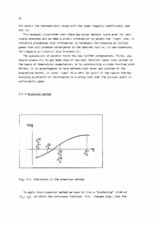
and select the thermodynamic state with the lower fugacity coefficient, see

ref. 61.

This example illustrates that there MY exist several mots even for very

simple problem and we need a priori information to select the 'right' me. In

iterative procedures this information is necessary for choosing an initial

guess that will p r m t e convergence to the desired r w t or, in me dimension,

for choosing an interval that brackets it.

The possibility of several rmts has two further consequences. First, y w

s h l d always try to get 5ome idea of how y w r function l w k s like, either M

the basis of theoretical expectation, or by constructing a crude function plot.

Second, it is advantagwus to have methods that never get outside of the

bracketing bcunds, or never "jump" to a very far pint of the region thereby

avoiding divergence or convergence to a wrong root whw, the initial guess is

sufficiently good.

2.1.2 Bisectim method

~

Fig. 2.1. Iterations in the bisection method

To apply this classical method we have to find a "bracketing" interval

[xL, xu] on which the continuous function f(x) changes sign, thus the

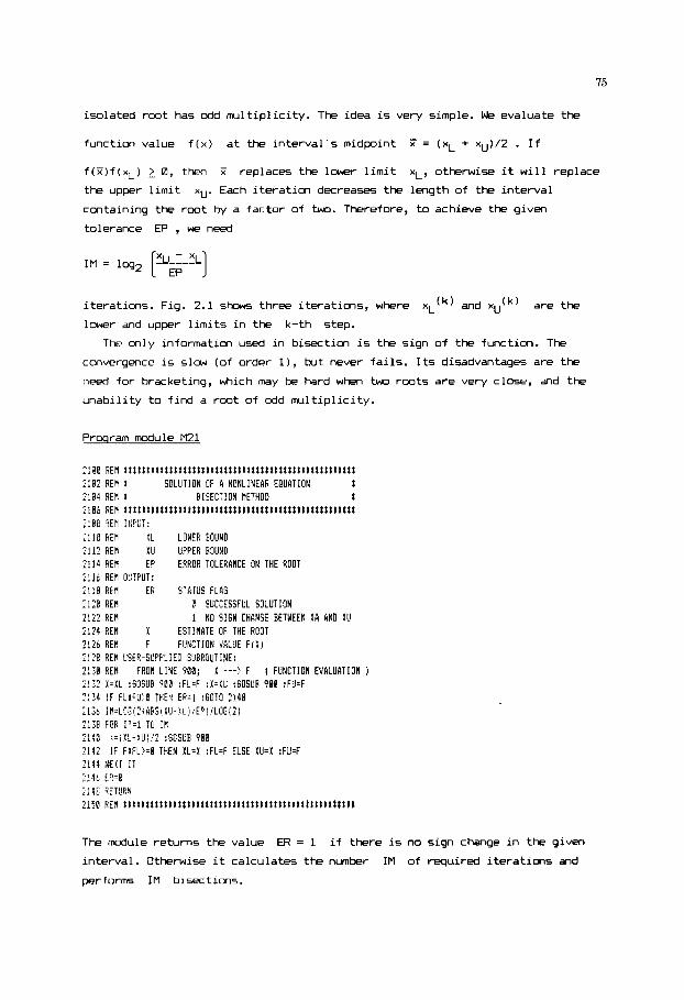
isolated r m t has odd rmltiplicity. The idea is very simple. We evaluate the

function value f(x) at the interval's midpoint iT = (xL + xu)/Z . If f(3)f(xL) 2 0, then 3 replaces the lower limit xL, otherwise it will replace

the upper limit

containing the root by a factor of two. Therefore, to achieve the given

tolerance EP , we need

xu. Each iteration decreases the length of the interval

iterations. Fig. 2.1 shanh three iterations, where

lower and upper limits in the k-th step.

x L ( k ) and xuCk) are the

The only information used in bisection is the sign of the function. The

cmvergmce is slow (of order 11, but never fails. Its disadvantages are the

need for bracketing, which may be hard when two roots are very close, and the

unability to find a r m t of odd multiplicity.

Prcqram m u l e MZ1

: l $ C FEM t t t t t ! t t t t t t t t t t t t t t t t t t t t t t t t t t t f t t t t t t t t t l t t t t t t t t t t ::I: REM 1 SCLUTIOP! OF A #ONL!NEAR EQUATION t 2104 REP f R!SEC'!OL! METHOD t ;1Cb HEY t t t t t l t t t t t t t t t t t t t t t t t t t t t t t t t t t t l t t t t t t t t t t t ~ t t t t t

21;O P i b lL LOWER BOUND :If: 6EE XU UPPER BOUND 2 1 1 4 QEE EP EFRCP TOLERANCE ON THE ROOT :!lt REH OLTPUT: 2 1 1 8 HEM ER STATUS FLAE :12E RE1 P SUCCESSFUL SOLUTION 2 1 2 2 RE1 1 NO SIGN CHANGE BETWEEN X R PND XU 2:4 RE!! k ESTIHATE OF THE HOOT 2 1 1 6 REE F FUNCTION JALUE F i k j

2 1 2 BEtl USEL-SUV',!EI~ S!IPRrJUT!NE: ?L70 HEN FROH L!NE 900; X ---' F ( FUIICTION EVALUATION ) 32 X=XL :GOSUB Y I I :FL=F :X=XU :GOSUB 98H :FU=F 2134 !F FLtFU 0 THEW EP.1 :GOTO ?!48 : I 2 I M = L I E I ? ~ A E S I Y U - ~ ~ ) E 0 ~ / t 0 6 [ ? ) 2138 'X I T = l TL IH Li13 :=iWL*XU! ? :GCSUE q@@

2142 !F FtFL'=R THEN PL=\ :FL=F ELSE XU=X :FU=F 1141 NEIT I T :!4t EP=& ::42 E T L I R I I ?lM PES t I t 1 t t t t t t t t t t t 1 t I I t t t t t t t 1 t t t t t t t t t I t t t t 1 t t t t t t t t t

;lee SEN w T :

The module returns the value ER = 1 if there is no sign change in the given

interval. Otherwise it calculates the number IM of required iterations and

performs IM bisections.

76

Example 2.1.2 Molar volume of n-buthane by bisection method

A l l methods i n t h i s section w i l l be tested by solving the problem presented

i n Example 2.1.1 . Rearranging ( 2 . 5 ) we have the function

a(T)

X ( X + b) + b ( x - b) ( X - b) - RT ,

where the solution of the equation f ( x 1 = 0 i s the molar volume. The simple

main program we use i s as follows.

This i s the f i r s t program i n t h i s b w k that needs a subroutine supplied by

the user. Each program intending t o c a l l the module M 2 1 must include EASIC

statements that evaluate the function f a t x. The f i rst l i n e o f the user

supplied w b r w t i n e i s l i n e Sew i f only one i s needed. Almost every program

further i n the bock w i l l require one, two or even three such subrwtines,

start ing a t l ines Sew, 800 and 7E0, respectively. Now you contribute t o the

program and hence i t i s advisable to include s m extra pr in ts i n the

subrwtines for debugging. Since there are no local variables i n BFISIC, you

s h w l d be careful when f i t t i n g user supplied subroutines t o more complex

program. Part icular ly dangerous is al ter ing values of the FOR-NXT loop

variables ( i n th i s case I T i s such a variable). To minimize the threat of

con f l i c t t r y t o distinguish your variables from ours, e.g. through the use of

variable names consisting of three or more l e t te rs i f your BASIC version does

accept such longer names. a user supplied subroutine i s always closed by a

RETURN statement.

In this example line 902 evaluates the function (2.6) and stores its value

in the variable F . We print X and F to follow the iteration. The

bracketing interval is chosen on the basis of a priori information. We know

that in this example the compressibility factor W/(RT) is close to me,

and use the lower and upper limits

where vo is the ideal molar volume

vo = RT/P . (2.7)

xL = v0/2 and xu = 2vo , respectively,

The error tolerance EP

smaller than the attainable accuracy based on the approximate equation (2.5).

h e to the PRINT statement in the user supplied subroutine the program output

is long, and only a few iterations are shown in Table 2.1.

is set to the value EP = ~~tlE-6 , which is certainly

Table 2.1 Steps in the bisection method

15 16 17 18 19 20

0.103417E-02

0.1421%-02

0.150512E-02 0.150521E-02 0.15052M-02 0.150528E-02 0.15053iE-02

0.41Jb69E-02 0.25854JE-02 0.16098eE-02

0.161590E-02

0.150531E-02

0.15053zE-02

+1 +1 -1 +1 +l

-1 -1 -1 -1 +1

2.1.3 False position method

Similarly to the bixticn method, we need an interval CXL, xu1 that

includes the root. The method is based m local linear interpolation of the

functim f by the straight line or chord through the points (xL, f(xL)) and

{xu, f(xU)>, as shown in Fig. 2.2. The "root" of this interpolating linear

functim is

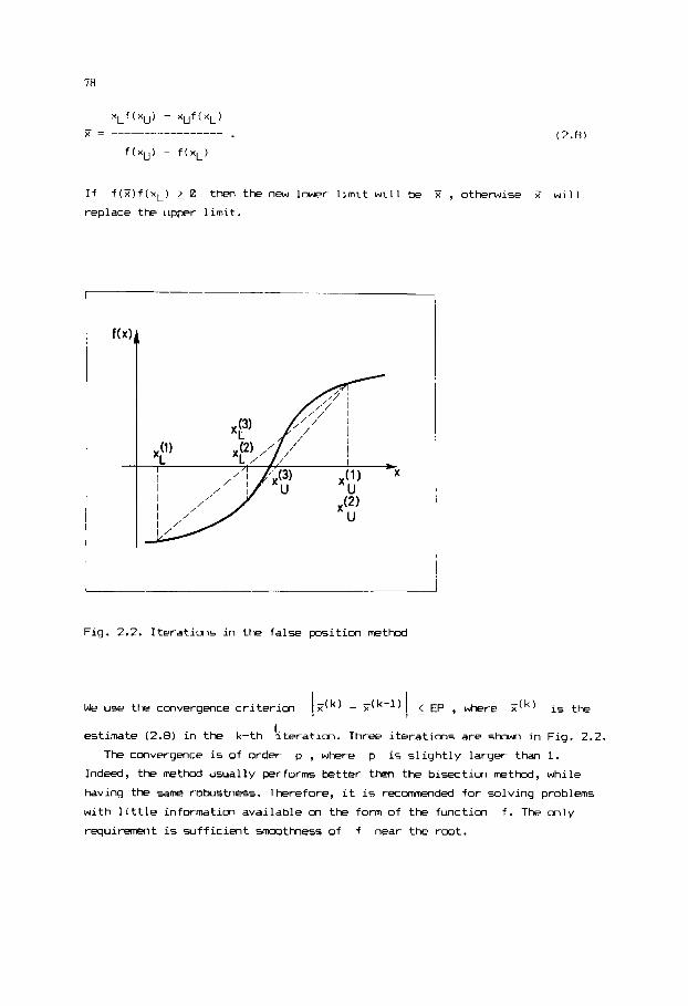
78

(2.8)

If f ( x ) f ( x L ) 2 0 then the new lower l i m i t w i l l be X , otherwise F w i l l

replace the upper l i m i t .

Fig. 2.2. I terat ions i n the false p s i t i o n method

use the convergence c r i t e r i on - r i ( k - 1 ) I < EP , where is the

estimate (2.8) i n the k-th ‘iteration. Three i terat ions are shown i n Fig. 2.2.

The convergence is of order p , where p i s s l i g h t l y larger than 1.

Indeed, the method usually performs better then the bisection method, while

having the same robustness. Therefore, i t i s recmmmded fo r solving problems

with l i t t l e information available on the form of the function f . The only

r e q u i r m t is suf f ic ient smoothess of f near the rwt.

79

Praqram module M22

2 3 8 K E N t t t t t t t t t t t t t t t t ! f t ! 1111 t t l f t I t t t t t t t t t t t t t t t t t t t t t 2202 CEM t SOLUTIGN OF R l O R L I N E R P EOUGTIO!1 t

2204 REfl t RE6:JLB FRLSI X T H C D t 72C6 REf l t t ! ! t t t t l t t t t t t l 4 t t t I f t t I t * t I t I t t t t t t t t t t t t I t t I t I t t X0t R E 3 !lPFT: !::$ :L LOI;EE $lLlY$

R E t XU UPPEf L3L;tjP 1214 @EM EP ERROR TCLEMdC-i 9EI TYE ROOT 2?lt REH 1% MNIkUE ?C!BBER 0; I T E R A T I O N S 2218 REf l OUTP!!T: 2 2 2 8 REF ER STATES F i A i 2222 REf l 0 SUCCiSSFOL SOLUTIf?N 7224 REI1 I 10 E I G N CHANGE BETWEEN XL AlD XU E b F'EM 2 REOLIPEC ACCURClCY NOT A T T A I N E D ?2?E REH Y ESTIMRTE DF THE ROUT 2230 AEM F FUNCTION I'dl!lf f ( 9 J 2232 REfl U S E R - S W L I E B S U B ? O U l I I E : 1254 REh FR?H L!HE 900; X ---: F I FUNCTION E V A L U A T I O N j 22% X=YL :GtOSUB 008 :FL=F :I=It! :68S?13 908 :FU=F 2 3 8 I F FLtFU)0 THEN ER=! : 6 0 T 3 225: 2248 FOR 11.1 T O I N 2247 XOzY : X = ( l L t F U - X U t F L i i l F l l - F l j :GOSUP 900 2214 I F F t F L : 4 THEN XL=X :FL=f E L S E XUzX :FU=F 2246 I F ABSIX-XG)<=EP THEN E R 4 :C;OTfl 2252 2248 NEXT I T 2250 ER=? 2252 RETURN 22S4 REt4 t t l t t t t l l t t l t t t t l l l l t t l l l t l t t ~ t 4 t l t t 4 t l t ~ ~ 4 t ~ t t ~

Example 2.1.3 Molar volume by f a l s e position method

The main p r q r a m is almost the same as i n

are i n the l i n e s listed below.

Example 2.1.2. The o n l y d i f f e r e n c e s

102 REN EX. 2.1.; NOLAR VULME B Y T A L E POSITION NETHOD

jN4 REt4 NERGE ti22

:'BE X L W t T T I P P I 2 :XU=RUtT!!YPf2 :EP=XUt.B000Bl : It4=70

214 GOSUB 2260

s i n c e w e have to s p x i f y t k number

m u l e NZ?. T h e iteratim prDce.s is summarized i n Table 2.2 , where the lower

and upper l i m i t s , the i nne r p o i n t and the corresponding f u n t t i m v a l u e are

sham i n each iteratim.

IM of allowed iteratims and cal l the

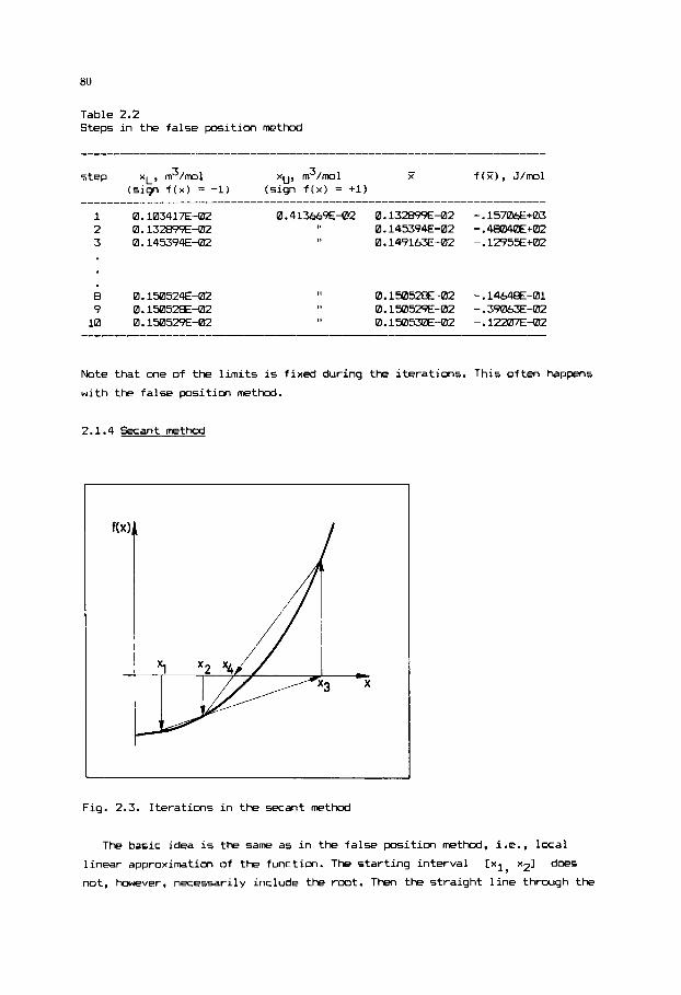
80

Table 2.2 Steps in the false position method

- f ( Z ) , J/ml X step xL, m3/m1 m3/m1 (sign f(x) = -1) (sign f(x) = +1)

1 0.103417E-02 0.413669E-02 2 0.132899E-02 3 0.145394E-02

8 0.1 E0524E-02 9 0.1!Xl52E-02

10 0.150529E-02

Note that me of the limits is fixed during

with the false position method.

2.1.4 Secant method

0.132assE-02 -.1570&+03 0.145394E-02 -.-mi02 0.149163E-02 -.12955€+02

0.15052E-02 -.14648E-01

0.1Yii53E-02 -.lZi07E-0)2 0.1 w529~-m2 - . 3 m ~ r n 2

the iterations. This often happens

Fig. 2.3. Iterations in the secant method

The basic idea is the same as in the false position method, i.e., local

linear approximation of the function. The starting interval

not, however, necessarily include the rwt. ThR, the straight line through the

Exl, x21 does

81

points Cxl, f ( x 2 ) ) and Cx2, f ( x 2 ) > extrapolates rather than interpolates

the function, and i t s "root"

w i l l replace the "older" of the two previous points, thereby always retaining

the most recent two estimates. (This requires an arbi t rary choice i n the f i r s t

i terat ion.) I f x2 i s the la test point, then x1 i s replaced by x2 and x2

by E , as shorn i n Fig. 2.3. The convergence cr i ter ion is again

Retaining the latest est imates for x1 and x2 , the slope of the l i n e

follows more closely the form of the funct im than i n the false positim

method. The order of convergence can be show t o be 1.618, the "golden rat io",

which we w i l l encounter i n Section 2.2.1. The root, hawever, i s not necessarily

bracketed, and the next estimate

f (x l )

search i n a region where the function i s not monotonic.

x3 may be f a r away i f the function value

i s close to f ( x 2 ) . Therefore we may run i n t o trouble when star t ing the

Prqram module M23

2300 REH t t t t t t t t t t t t t t t t t t l l t l t t ~ t t t t ! t t t l t & t t t t t t t t t l t t t t t t t t 2 3 0 2 RE! t SOLUTION OF A NONLINEAR EQUATION t 2304 REH t SECANT HETHOD t 2 3 0 6 REH t ~ t t t l l t t t t t t t t t t t t t t t t t t t t t t t l t ~ t t t t t l l t l t l t l l l t t k 2308 REfl INPUT: 2 3 1 0 REII X I I N I T I A L ESTIIIATE OF THE ROOT 2312 REH Y ? SECOND I N I T I A L ESTIIIATE OF THE ROOT 2 3 1 4 REfl EP ERROR TOLERANCE ON THE ROOT

2 3 1 8 REH OUTPUT: 2320 REM ER STATUS FLAG 2322 REfl D SUCCESSFULL SOLUTION 2324 REM 1 REQUIRED ACCURACY NOT ATTAINED 2 3 2 6 RE! 2 ZERO SLOPE 2328 RE1 X ESTIMATE OF THE ROOT 2330 REII F FUNCTION VALUE F I X ) 23!2 PER USER SUPPLIED SUBROUTINE: 21.34 REF FHOII L I N E 900; X ---) F ( FUNCTION EVALUATION ) 2336 X = X I :GOSUB 900 : F l = F :X=X2 :GOSUB 900 :F2=F 2?38 FOR l T = l TO I N

2316 REH IH NAXInun NUHBER OF ITERATIONS

2340 2342 X = ( X l t F 2 - X 2 t F l ) / ( F 2 - F 1 ) :GOSUB 980

I F AES(F?-FI)!lE-30 THEN ER.2 :GOTO 2352

2344 IF BBS(X-XZ)(:EP THEN ER=B :GOTO 2352 2346 Xl=XZ :Fl=F2 :XZ=X :F2=F 2 . 3 8 NEXT I T 2 3 0 ER.1 2352 RETURN 2214 RE! t t t t l t t t t l t l t t t t t t t t t t t t t ~ t t t t t l t t t t t t t t t t t t t t l t t t l

82

kcord ing to (2.9) the method breaks down i f

i terat ions. Then the module returns the value ER = 2 . f (x l ) = f ( x 2 ) i n any one of the

Example 2.1.4 Molar volume by secant method

We deliberetely do not "bracket" the rwt and use the i n i t i a l estimates

x1 = vo and x2 = 1 . 0 1 ~ ~ , where vo i s the m l a r volume calculated f rom the

ideal gas law (2.7). The i terat ion i s expected t o converge t o the root

correspcnding to the gaseous state. We do not present the main program, because

the deviations from the previous two main prqrams are only i n the l ines:

102 REIC EX. 2 . 1 . 2 MOLBF! VOLUME BY SECANT METHOD

184 PEN IIEKE HF

Z08 Yl=RUtTT/PF : X 2 = 1 . O l t R U t T T / P P :EF~Xlt.000001 : Itl=30

214 GOSUP ?!00

i.e., we have t o specify X 1 and X 2 instead of XL and XU . Results are l i s ted

i n Table 2.3.

Table 2.3 I terat ions i n the secant method

1 0.22&835E-m 0.200703E-02 0.155446E-02 0.4754e€+02 2 0.2GEmaE-02 0.155446E-02 0.151126E-02 0.568J3E+01 3 0.15544M-02 0.151 126E-02 0.150539E-02 0.86914E-01 4 0.15112M-02 0.150539E-02 0.1505311E-02 0.24414E-03 5 0.1 m39E-02 0.13053E-02 0.1505311E-02 -.24414E-03

The idea i s again local l inear approximation, but now w e use the tangent

l i ne a t a current estimate x of the root. The tangent l i n e w i l l cross the

zero a t the abscissa

f ( X ) - x = x - ---- 9

f ' ( x )

(2.10)

where f ' ( x ) i s the derivative o f function f a t x , and w e adopt R as the

next estimate.

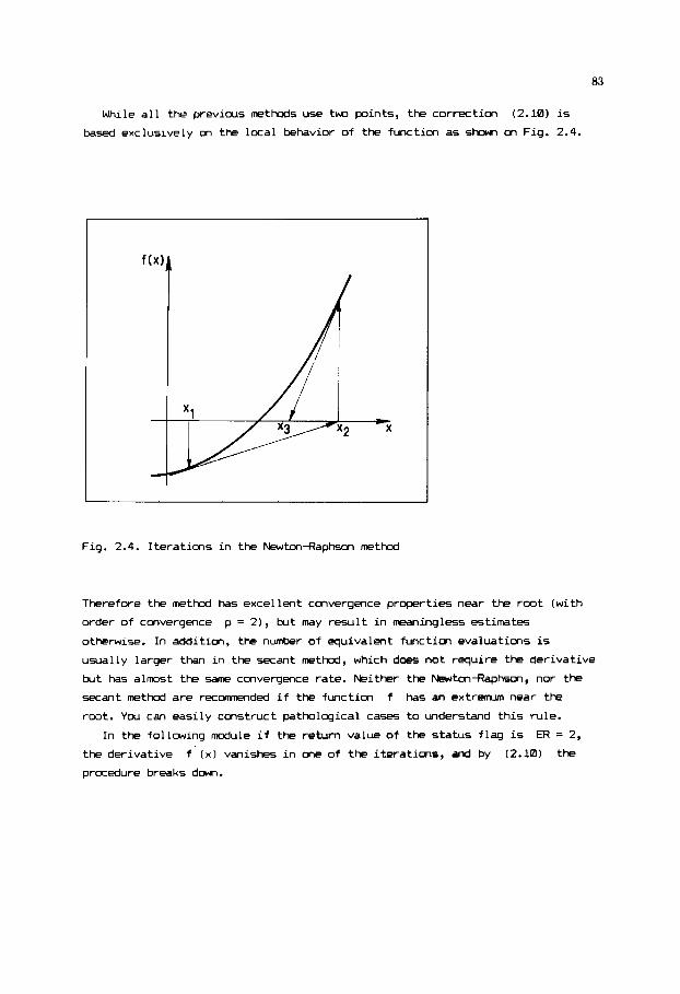
83

While a l l the previous methods use two points, the correction (2.10) i s

based exclusively on the local behavior of the function as show, on Fig. 2.4.

Fig. 2.4. Iterations i n the Newtm-Raphsm method

Therefore the method has excellent convergence properties near the root (wi th

order of convergence

otherwise. I n addition, the number of equivalent function evaluations i s

usually larger than i n the secant method, which does not require the derivative

but has almost the same convergence rate. Neither the Newton-Rapkon, nor the

secant method are recommended i f the function f has an extremvn near the

root. Y o u can easily construct pathological case5 t o understand th i s rule.

the derivative f ’ ( x 1 vanishes i n one of the i terat ions, and by (2.10) the

procedure breaks down.

p = 21, but may result i n meaningless estimates

I n the following module i f the return value of the status f lag i s ER = 2,

84

Proqram module MZ4

2400 REM t t t t t l ~ & t t t ~ l t t t t t t t ~ l l t l l l l t l l t t l l l l l & l t l l t t l l t & t ~ 2402 REtl t SOLUTION OF A NONLINEAR EQUATION t 2404 RE\ t NEWTON-RAPHSON METHOD t 2406 REM l t t t t t ~ t t t t t t t l & t f t & l t l t t t t t t t t t t t l t t l t l t t t t l l l ~ l l l l l l 2488 RE1 INPUT: 2416 REH X I N I T I R L ESTl t lATE OF THE ROOT 2412 RER EP ERROR TOLERANCE ON THE ROOT 2414 REtl In NAXlflUtl NUMBER OF ITERATIONS 2416 RE! OUTPUT: :41E REIl ER STATUS FLA6 242C REW 0 SUCCESSFUL SOLUTION 2422 REH 1 REQUIRED ACCURRCV NOT ATTAINED 2424 REW 2 ZERO SLOPE 2426 RE1 X ESTIHATE OF THE ROOT 2426 RER F FUNCTION VALUE FIX) 2431 BEN USER-SUPPLIED SUBROUTINE: 243: REN FRO# L I N E 90B; X ---) F ( FUNCTIUM EVALUATION ) 2434 REIl FRO\ L I N E 800; X ---> D 1 DERIVATIVE EVALUATION )

2436 GOSUB 900 2438 FDR 11.1 T@ I M 2440 GOSUB 800 2442 I F A E S ( D ) c l E - M THEN ER.2 :60TO 2452 2444 DX=-F/D :X=XtDX :GOSUB '400 2446 I F ABS(DX)!=EP THEN E R 4 :60T@ 2452 2448 NEXT I T 2450 ER.1 245: RETURM :454 REH t t ! t t l t l l t l l l t l l l t t l l t t t t l t t t t t t t t t t t t t t t l l t l l l l l l l

Example 2.1.5 Molar volume by Newtcn-Raphsm method

To use the m u l e MIL4 y w should supply two subrou t ines . As i n the p r e v i w s

methods t h e one s t a r t i n g a t l i n e CMW w i l l e v a l u a t e t h e va lue F of t h e

funct ion. T h e second s u b r w t i n e , s t a r t i n g a t l i n e Sena, g i v e s t h e c u r r e n t va lue

of the d e r i v a t i v e f ' ( X I

s i n g l e i n i t i a l guess X . Chce again we u s e t h e i d e a l gas volume a5 i n i t i a l

estimate. T h e l i n e s d i f f e r e n t from the l i n e s of t h e previous program are:

t o the v a r i a b l e D . To s ta r t the i t e r a t i o n we need a

8Ba REW ---------- DERIVATIVE 682 D=PFtAE/ (XI (X+BE)+BEt IX-BE) ) - l X - B E ) t A E l i 2 t X t 2 & B E ) / ( X t ( X + B E ) t B E & ( X - ~ E ) )^2 804 RETURN

R e s u l t s are shown i n Table 2.4.

85

Table 2.4 Iterations i n the Newtondapkon method

A br ie f comparison of the di f ferent methods i s given i n Table 2.5. You may

notice that the methods that use m r e informatim (i.e., the value o f the

function, not only i t s sign; a pair of values, not m l y one of them) converge

more rapidly. Y o u already know, her, that robustness i s decreasing along

the same l ine. Therefore, choosing a method you ought t o cmsider h w nuch i s

k n m on the form of the funct im and the position o f i t s roots.

Table 2.5

Convergence behaviour of the di f ferent methods i n the test example

Method MJmber Munber of equivalent Theoretical order of of i terat ions function evaluations cmvergence, p

--------------_---____I___ I--

Bisection 19 21 1 False position 10 12 >1 Secant 5 7 1.6 Newton-Raphson 4 9 2 ------_--__----__I_I___- ---I__

2.1.6 Successive approximation

This method has such poor convergence properties that i t i s usually omitted

from up-to-date textbooks m numerical analysis. We mention it, however,

because i t i s very simple and s t i l l i n use. I n addition, the method can be

easily extended t o systems o f equations where i t is the basis fo r a number of

improved techniques. The idea i s wr i t ing the equation i n the form

(2.11)

and performing the i terat ion

where x and Z are the old and new guesses of the rwt, respectively. A

suf f ic ient condition for convergence i s the existence of a constant K < 1 and

86

of an interval arwnd the root on which

if cur initial guess is also in this iterval. The steps of this procedure, also

k n w as direct iteration, can be well follDved on plots like the ones shown in

Fig. 2.5. The 45' straight line helps to convert a

guess si . You may encwnter the situations of monotonic or oscillating

convergence (Fig. 2.5.a and b, respectively) and monotonic or oscillating

divergence (Fig. 2.5.c and d, respectively).

g(x) value into a new

YA

y-g(x)

X '1 '2'3

a

yk; yk=x

x3 x2 x1 X x3 x1 K2

Fig. 2.5. Typical situations in successive approximation

87

I t i s m r e d i f f i c u l t t o judge the properties of successive approximation i f

the or ig inal equation i s of the form f ( x ) = 0 , since i t can be rearranged t o

the form (2.11) i n many d i f ferent ways, thereby s ign i f icant ly influencing the

convergence. For example, an appropriate r e a r r a n g m t resul ts i n (2.103, and

hence even the Newton-Rapkm method can be regarded as successive

approximation.

Exercises

0 Derive the i terat ion formulas (2.81, (2.9) and (2.10) on the basis of the

geometrical ideas used i n the corresponding method.

0 Solve the test problem of t h i s section a t the pressure P = 1.6x10' Pa

keeping i n mind that now the n-tuthane i s i n l iqu id state.

0 Three r e a r r a n g m t s of equation (2.5) t o the form x = g(x) are:

g2(x) = RT/P(l + a/P/Cx(x + b) + b(x - b) l ) - ' + b

Try to solve the test problem by successive approximation on the basis of

these rearrangements. What i s the reaKn of divergence i n the ca5e of g3 ?

2.2 M I N I M a " C T I O N S IN ON DIMNSION

Similarly t o the most robust methods of solving nonlinear equations, we

s ta r t with bracketing. Assume that the interval

minirmm point r, i.e., the function f i s decreasing up t o r and increasing

afterwards. Then the function i s said to be u n i d a l on the interval [xL, xu].

This property i s exploited in cut-of f methods, plrported t o reduce the length

of the interval which w i l l , however, include the minirmm point i n a l l

i terations.

[xu, xL] contains a single

The idea we use i s s imi lar t o bisection, but now we need t o evaluate the

function at two inner points

xL < x1 < x2 < xu. I f

ExL, x21 , since we assumed that the function i s decreasing up t o the mini-

point, see Fig. 2.6.a. Similarly,

x1 and x2 of the interval , where

f(x l ) 5 f ( x 2 ) , then the minimum point i s i n the interval

f(xl) 2 f (x2) implies that the minimum

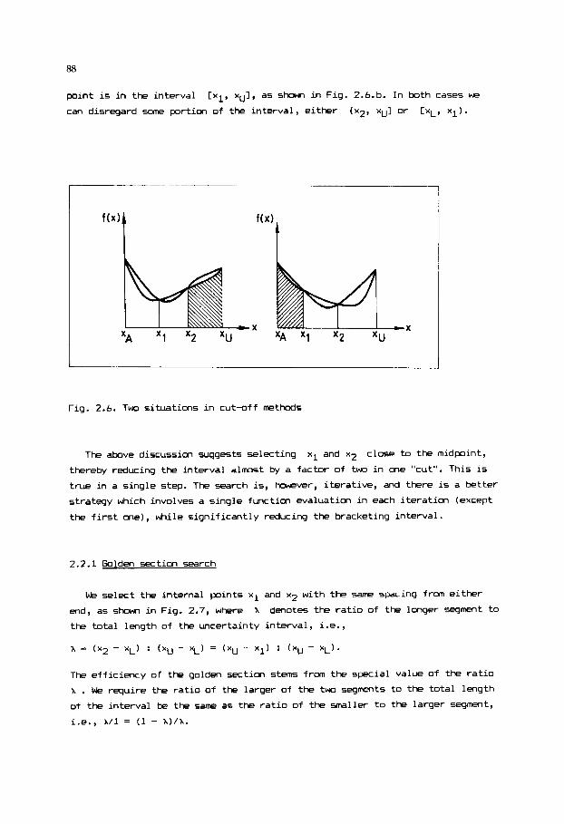
88

point is i n t h e i n t e r v a l

can disregard 5ome portion of the i n t e r v a l , e i t h e r

[x l , xu], as show, i n Fig. 2.6.b. In both cases we

( ~ 2 , xu] or C X L , x i ) .

Fig. 2.6. Two s i t u a t i o n s i n cut-off methods

The above discussion sugges ts s e l e c t i n g x1 and xz close to t h e midpoint,

thereby reducing the i n t e r v a l a l m t by a f a c t o r of two i n one "cut" . This is

t r u e i n a s i n g l e s t e p . The search is, however, i t e r a t i v e , and there is a better

s t r a t e g y which involves a s i n g l e funct ion evaluat ion i n each i t e r a t i o n (except

t h e f i r s t me), while s i g n i f i c a n t l y reducing t h e bracket ing i n t e r v a l .

2.2.1 Golden sec t ion search

We select t h e i n t e r n a l p i n t s x1 and x2 with t he same spacing frcm e i t h e r

end, as show, i n Fig. 2.7, where

t h e total length of the uncer ta in ty i n t e r v a l , i.e.,

X denotes t h e ratio of t h e longer segment to

-A = (x2 - X L ) : ( x u - XL) = ( x u - X I ) : ( x u - X L ) .

T h e e f f i c i e n c y of t h e golden s E t i o n stem f r m the special va lue of the ratio

X . We requi re t h e ratio o f t h e l a r g e r of t h e two segments to the total length

of t h e i n t e r v a l be t h e same as the ratio of the smaller t o t h e l a r g e r segment,

i.e., ?J1 = (1 - h)/X.

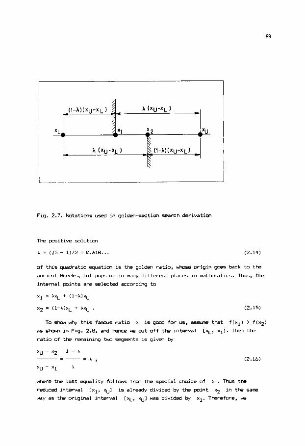
89

Fig. 2.7. Notations used in golden-section search derivation

The Dositive solution

A = ($5 - 1) /2 = 0.618... (2.14)

of this quadratic equation is the golden ratio, w h o s e origin goes back to the

ancient Greeks, but pops up in many different places in mathwMtics. Thus, the

internal points are selected according to

x 1 = AXL + ( l - X ) X u

x 2 = ( l - A ) x L + AXu . (2.15)

To show why this f m s ratio A is g w d for u5, assume that f(xl) > f ( x 2 )

as shown in Fig. 2.8, and hence we cut off the interval

ratio of the remaining two segments is given by

[XL, XI). Then the

(2.16)

where the last equality follows from the special choice of A . Tt-us the reduced interval [xl, xu] i5 already divided by the point x2 in the same

way as the original interval [xL, xu] was divided by xl. Therefore, we

90

replace xL and x1 by the old value of

evaluate the function only at the new point

Fig. 2.8 shows how the roles of our four points have been changed w h e n

performing this step. Similarly, for

interval is [xL, x21 and thus we replace xz and xu by x1 and xz , respectively, and evaluate the function at the newly selected

x1 and xz , respectively, and need to x2, selected again by (2.15).

f(x1) < f(x2) the new bracketing

xi.

X

Fig. 2.8. Steps in the goldm-section search

The golden section search guarantees that each new function evaluation will

reduce the uncertainty interval to a length of X times the previous interval.

This is comparable to, but not as g d as interval halving in the bisection

method of solving a nonlinear equation. Y o u can easily calculate that to attain

an error tolerance EP we need

iterations. The following module calculates IM and performs the iterations.

91

Proqram module M25

301 PER ttttttttttttttttttttttttttttttt~tttittttttttttttttt

;554 R i n t BETHOD OF GOLDEN SECTIONS t :'& PEfl I t t t t t t t t t t t t t t t It t t t t t t t t t t t t t I t t t t t t t t 1 t t t 1 t t t I It

REM t M I N I W M OF A FUNCTION OF m E V ~ R I A P L E t

2568 EEN INFUT: 2 x 8 HEM x i LOWER POUND 251: HEN Y U UPPER houw

:sie FEN x ESTIMATE OF THE MINIHUH POINT

3 1 4 RE1 EP ERROP TCLEPANCE ON HINIMUM POINT 151b REH CUTPUT:

252e REM F #INIMU! FUNCTION VPLUE F(W) 2 S Z RE! USER-SUPPLIED SUBROUTINE 2521 HEM FXI)M L I N E 9 0 8 ; X - - - ) F I FUNCTION EVALUPTIOl 1 iYC PL= I S X ( 5 ) -1 ! i 2 : RUZl-HL : RE:l IRL 2 5 2 I f l=LOG(REtAES( XU-XL) !EP) ILOG(RE) 3 5 8 21=RLtYL+RUtXU :$=XI :GOSUB 900 :F l=F 25;: X?=RUtXL+RLtYU :l=!: :GOSUP 700 :F?=F i5!4 FOF. 11.1 TO I R .5h I F FI'FZ i h E N 2512 23 tJ=i: : Y l = X l : F X l :Xl=RLtYL+RUtXU : X = X l :GOSUR 900 :F l=F 2 5 4 6 SOTO :544 254: !:=XI : Y I = X ? : F l = F ? :X?=RUtXLtRLtXU :X=X2 :GOSUP 900 :F?=F 3 4 4 NEi ' IT 2 5 4 6 PiTUFN ?SJ8 PEfl tttttttttttttttttttt~ttttt!tttt~tttttttttttttittttF

- 7

The mdu le needs a user supplied r w t i n e s ta r t ing a t l i n e W that w i l l set

the variable F to the value of the function evaluated a t the actual value of

x .

Example 2.2.1 Optimal drug dosing by golden section search

Consider a tab le t that i s taken regular ly once a day. We want t o f i n d the

optimal quanti ty of the drug (i.e., the only act ive ingredient) i n the tablet

i n order t o keep the drug concentration i n the b l d w i th in a given therapeutic

range

use the l inear compartmental model shmm i n Fig. 2.9, me of the most p o p l a r

models i n pharmacokinetics.

[cL, cul as s t r i c t l y as possible. To predict the drug concentration we

The model assumes that the drug enters compartment 1, representing mainly

the gastrointest inal t rac t . The drug i s then absorbed i n t o the blood f low,

represented by compartment 2 . The absorption ra te i s kaql , where q1 i s the

current drug quanti ty i n compartment 1. There i s also a secretion o r

e l im ina t im process f rom compartment 2, w i th the el iminat ion ra te

q2

kq2 , where

denotes the quanti ty of drug i n compartment 2.

92

Fig. 2.9. Pharmacokinetic compartmtal rodel

1 - gastrointestinal tract; 2 - blood flow

The compartmental &el gives rise to a system of two linear differential

equations whose forcing term (i.e., the drug intake) is a periodic function

(ref. 9). After a transient period the solution of the differential equations

is also a periodic function. This periodic solution predicts the drug

concentration

(2.17)

where D denotes the dosis, i.e., the quantity of drug in the tablet (q); V

is the distribution volume of the blood compartment;

coefficient; k is the elimination rate coefficient; 7 is the period, i.e.,

the time elapsed betmen two intakes of the tablet, and t is the time

elapsed after the latest intake. In this example

k = 0.a93 h-l and

k, is the absorption

V = 10 1, k, = 0.231 h-',

7 = 24 h (ref. 9).

We want to find the value of D that will keep c(t) between the values

cL = 14 mg/l and cu = 26 mg/l minimize the objective function

as far as possible. For this p r p e we

93

7

f(D) = (1/7)[[hz1(t) + hZ2(t)]dt (2.18)

where

thereby more penalizing concentration values far from the therapeutic range.

The area contributing to the objective function is shaded in Fig. 2.10.

Fig. 2.10. Periodic drug concentration in blwd

Y w are certainly aware that the compartmental &el is a simplified

representation of the real physicological process. Therefore, it is completely

adequate to use a simplified objective functim by approximating the integrals

in (2.17). We divide the interval 10, 71 of integration into W equal

subintervals of length At = 7/W , and approximate c(t) by its midpoint

value ci = cC(i - 1/2)Atl. The objective function is approximated by

(2.19)

94

where

[(ci - cu) 'At i f ci > cu

(cL - c i ) ' A t i f ci < cL

0 otherwise .

Since t h e d o s i s D

a t c e r t a i n t ime p o i n t s , from the approximate balance e q u a t i m

have D 5 260 mg . Therefore , the i n i t i a l i n t e r v a l [0, 10D23 c e r t a i n l y

inc ludes the minimm p o i n t , which can be e a s i l y c h e c k e d e v a l u a t i n g the func t ion

(2.19) over a cour se g r i d . T h e d e s i r e d error t o l e r a n c e is EP = 0.1 , more than

adequate i n t h i s problem. The main program we u s e is as follOW5.

is e x p e c t e d to raise the blood concmtratim a t least to cu

D/V z cu we

95

The limits of the uncertainty interval in some of the iterations are show

Table 2.6. The optimal dosis is Dopt = 335.4 mg , which gives the minimum value f(Dopt) = 14.44 (q21-2s).

in

Applying a finer grid (Nw > 48) does not alter the location of the minimum

m r e than the desired tolerance EP = 0.1 mg . In Fig. 2.10 we have already

shown t k concentration of the drug following the dosis

beginning of each period of length T = 24 h. kcording to this solution, one

tablet a day does not enable us to keep drug concentration

therapwtic range for all times. We could decrease the period, i.e., T = 20 h

wwld be a suitable choice, but it is not a practical advice to take a tablet

each 20 hours. Taking two tablets a day (i.e., with T = 12 h), there exists an interval CDL, DU1 such that f(D) = 0 for all D in this interval. F r a

physiological point of view the best choice is 9, i.e., the least dosis that

gives the desired drug concentration in blood. The golden section search d u l e

as presented here will result in this lower limit (4 = 138.2 mg) because in

line 2536 we used the relatimi sign ">" and not ">=" .

Dopt, taken at the

c(t) within the

Table 2.6 Steps in the golden section search

step XL, mg xu3 mg relation of fl to f2

1 0 2 3 236.M 4

10DZI 418.034

472.136

18 335.275 335.555 > 19 335. J82 < final 335.489

Although the golden section search works quite w e l l , it is obviously not the

best available for a given number of function evaluations. For example, with

only two evaluatims allowed it is better to choose the internal points close

to the midpoint of the initial interval, as we already discussed. The idea can

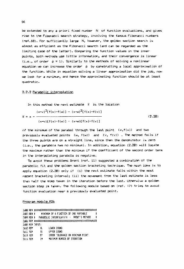
96

be extended to any a priori fixed number N of function evaluations, and gives

rise to the Fibmacci search strategy, involving the f m s Fibonacci numbers

(ref.10). For sufficiently large N, hOwever, the golden section search is

almxt as efficient as the Fibonacci search (and can be regarded as the

limiting case of the latter). Comparing the function values in the inner

points, both methods use little information, and their ca-ivergence is linear

(i.e., of order p = 1). Similarly to the methods of solving a nonlinear

equation we can increase the order p by constructing a local approximation of

the function. While in equation solving a linear approximation did the job, now

we look for a mininum, and hence the approximating function should be at least

quadratic.

2.2.2 Parabolic interpolation

In this method the next estimate F is the laation

( x-vpc f ( x ) -f (w 11 - ( x-w) 2c f ( x ) -f (v) 1 - =

(x-v)[f(x)-f(w)l - (x-w)Cf(x)-f(v)l (2.20)

of the m i n i m of the parabol through the last point Cx,f(x)3 and two

previously evaluated points <w, f(w)) and Cv, f(v)> . The method fails if the three points are on a straight line, since then the dmaninator is zero

(i.e., the parabola has no minimum). In addition, equation (2.20) will locate

the maximum rather than the minimum if the coefficient of the second order term

in the interpolating parabola is negative.

To avoid these problerm Brent (ref. 11) aggested a canbination of the

parabolic fit and the golden section bracketing tRhnique. The main idea is to

apply equation (2.i0) only if (i) the next estimate falls within the most

recent bracketing interval; (ii) the movement frm the last estimate is less

than half the step taken in the iteration before the last. Otherwise a golden

section step is taken. The follcwing module based on (ref. 12) tries to avoid

function evaluation near a previously evaluated pint.

Prwram module M26

ib0B REH t t t t t t t t l t l t t t t l t l l t l l t t t t l t t l l ~ ~ t ~ l l l ~ l ~ l t l t t t t t ~ l ?b0? REM 1 I 2604 REM t PARABOLIC INTERPOLATIDN - RRENT'S NETHOD t 2506 RE! ~ t t t t ~ t ~ ~ t l t t t t l ~ l t t l l l t l l l l ~ t t l t ~ l l ~ l l l l ~ l t l ! l ~ l ~ l 2608 REH INPUT: 2b lB REM XL LOUEF! BOUND 2512 REtl XU UPPER BOiiND 2614 REM EP ERROR TOLERANCE ON BINIHUH POINT ? b l b REIl IN tlAxlMUH NUMBER OF ITERATION

HINIHUM OF A FUNCTION OF ONE VAHIPBLE

97

2 6 1 8 REM OUTPUT: 2620 RE4 X ESTIflBTE OF THE f l I N I H U 1 POINT 2622 REH F MINIMUIi FUNCTION VALUE F ( X ) 2624 RE1 ER ST4TUS FLAG 2626 REM 0

2630 HEM USER-SUPPLIED SUBROUTINE 2632 RE1 FRO\ L I N E 901; X ---) F ( FUNCTION EVALUATION 1 2634 ER.8 :RL~(SQR(S)-l)/2 :DI=(XU-XL) /2 :X=(XU+XL)/2 76% V = X : W = X :E=0: GOSUE 900 :FX=F :FV=F :F&F 263P REM ----- LOOP 2640 FOR I T = l TO I f l 2642 2644 I F ABS(E)(EP THEN 2664 2646 2649 23550 Q = ? t ! Q - R ! : I F 0:>=0 THEN P=-P ELSE 0.-0

2 6 3 REH 1 TOLERANCE NOT ATTAINED IN ' Ins ITERATIONS

! M ~ ( X L t X U ) i 2 : I F ABS[X-Xn)i=2tEP-(XU-XLI I2 THEN 2696

RER ----- AUXILIARY QUANTITIES TO A PARABOLIC STEP Rz ( X - W ) t (FX-FV) : Il=( X-V! 1 (FX-FIJI : P'( 14') tQ-( X - W 1 tR

2152 EL=E :E=DX 2654 2656 REH ----- PARABOLIC STEP 2658 DX=F'/Q : U = l t D I 26t.8 I F ( U - X L ) < ? t E P OR (IU-U)!:tEP THEN I F Xn:}X THEN DX=EP ELSE DXz-EP 2662 GOT0 2678 2664 HEM ----- GOLDEN SECTION STEP 2666 I F X ) = X I I THEN E.1L-X ELSE E.1U-X

2678 RE! ----- FSNCTION EVALUATION 2672 2674 X0:Y :X=U :GOSUB 9 8 8 :FU=F : X = k O 2676 2678 I F F U N THEN 2684 2 6 8 8 IF UI=X THEN XL=X ELSE XU:X 2682 V=W :FV=FW : W = X :F#=FY :X=U :FY=FU :GOTO 2692 2684 I F U%'X THEN XL-U ELSE XU=U 2686 I F FU!FW AND #<:I THEN 2690 2 6 8 8 V=W :FV=FW :W=U :FW=FU :GOTO 2692 3 9 8 I F FU.=FV OR V = X OR V=W THEN V=U :FV=FU 2692 NEIT I T 2694 ER.1 2696 F=FB :RETURN rb?s REH l t t : t t t t t l r t t t t t t t t t t t t t t l t t t t t t t t t t t t t t t t t t ~ t t : I t t

I F APS(P))=ABS(QtEL/2) OR P i = Q t ( X L - X ) OR P)=QtlXU-X) THEN 2664

2668 DXzRLtE

I F ABS(DX):=EP THEN U=XtDX ELSE I F DX;B THEN U=XtEP ELSE U=X-EP

REM ----- NEbi BRACKET AND PREVIOUS POINTS

The i n p l t to the module is similar to the me of t h e module M25. T h e on ly

d i f f e r e n c e is that i n t h i s case the maximm number IM of iteratims should

be s p e c i f i e d be fo re c a l l i n g .

Example 2.2.2 Optirmm dosing by B r e n t ' s method

We s o l v e the problem of Example 2.2.1 wi th the same s t a r t i n g i n t e r v a l . T h e

main program is e s s e n t i a l l y the same excep t the fol lowing l i n e s :

208 XL.0 :YU=180@ :EP=. l :IM=38

714 L P R I l T V1 :LPRINT :LPRINT "BREIIT'S flETHOD' :LPRINT

216 GOSUB 2600

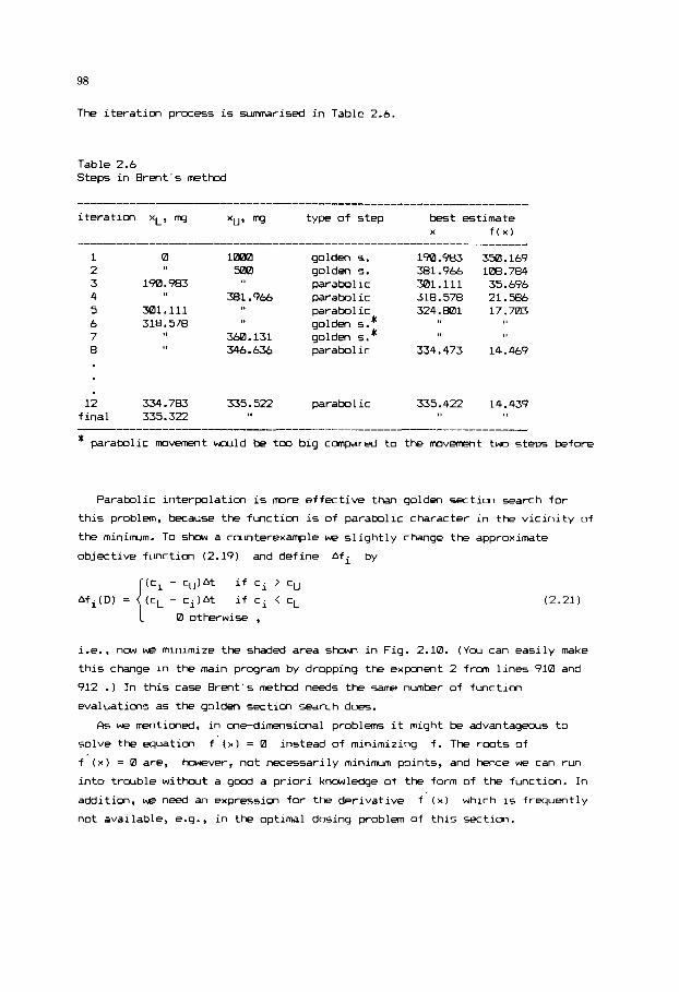
98

The iteration process is m a r i s e d in Table 2.6.

Table 2.6 Steps in Brent's method

iteration xL, mg

--------I---------

1 0 2 3 190.983 4 5 331.111 6 318.578 7 8

xu, mg

10ZGl w.2

381.966

360.131 346.636

type of step

golden 5 .

golden s. parabolic parabolic parabolic golden 5.'

golden s.' parabolic

best estimate X f(x)

190.983 350.169 381.966 lB8.784 301.111 35.696 318.570 21.586 324.801 17.703

334.473 14.469

12 334.783 335.522 parabolic 335.422 14.439 final 335.322

* parabolic mv-t would be too big compared to the m v m t two steps before

Parabolic interpolation is more effective than golden section search for

this problem, because the function is of parabolic character in the vicinity of

the minirmm. To 5how a cwterexample we slightly change the approximate

objective function (2.19) and define Afi by

- cU)At - ci)At

if ci > cu if ci < cL

0 otherwise , (2.21)

i.e., now we minimize the shaded area show in Fig. 2.10. ( Y w can easily make

this change in the main program by dropping the expent 2 from lines 910 and

912 . ) In this case Brent's method needs the same number of function

evaluations a5 the golden section search does.

As we mentioned, in one-dimensional problems it might be advantageous to

solve the equation f (x) = 0 instead of minimizing f. The roots of

f ( x ) = 0 are, b v e r , not necessarily minimum points, and hence we can run

into trwble without a g o d a priori knowledge of the form of the function. In

addition, we need an expression for the derivative f (x) which is frequently

not available, e.g., in the optimal dosing problem of this section.

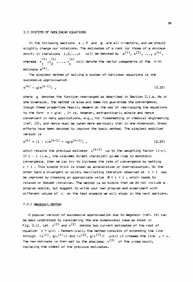
99

2.3 SYSTEMS OF NavINAR EWTIONS

In the following sections x , f and g are all n-vectors, and we'shwld

slightly change cur notations. The estimates of a r m t (or those of a minimum

point) in iterations 1,2 ,..., k will be denoted by x(l), x('), ..., X(k), ,..., x ( ~ ) will denote the vector cmpments of the k-th

(k) (k) 1 'x2

whereas x

estimate x(k).

The simplest method of slving a system of nonlinear equations is the

successive approximation

.(k) = 9 ( (k-1) ) , (2.22)

where g denotes the function rearranged as described in Section 2.1.6. As in

me dimension, the method is slow and does not guarantee the convergence,

t b g h these properties heavily depend on the way of rearranging the equations

to the form x = g(x) . It is, hDwever, extraordinarly simple and hence convenient in many applications, e . g . , for flowsheeting in chanical engineering

(ref. 13), and hence must be taken more seriously than in one dimension. Great

efforts have been devoted to improve the basic method. The simplest modified

version is

(2.23)

which retains the previous estimate

If c = 1 (i.e., the simplest direct iteration) gives rise to motonic

convergence, then w e can try to increase the rate of convergence by setting

c > 1 . This simple trick is known as acceleration or overrelaxation. !3 the other hand a divergent or wildly oscillating iteration observed at c = 1 may

be improved by choosing an appropriate value 0 < c < 1 , which leads to relaxed or damped iteration. The method is 50 simple that we do not include a

program module, but suggest to write your own program and experimnt with

different values of c on the test example we will study in the next sections.

x(~-') up to the weighting factor (1-c).

2.3.1 Wwstein method

A popular version of successive approximation due to Wegstein (ref. 14) can

be best understwd by considering the one dimensional case as shown in

Fig. 2.11. Let

equation x = g(x) . Gewnetrically the method consists of extending the line

through {x(l), g(x(l))) and {x('), g(x(2))> until it crosses the line y = X.

he new estimate is then set to the abscissa

replacing the oldest of the previous estimates.

x(') and x(') denote two current estimates of the r m t of

x(3) of the cross point,

100

Fig. 2.11. Gwmetric idea o f the Wegstein method

Therefore the above expression provides an a u t m t i c selection of the damping

or accelerating factor c i n each i terat ion. The idea i s easy to extend t o a

system of equations, i f each element xi o f the vector x i s regarded t o be

independent of the others w h w , using the expressims (2.23) and (2.24) . Thus

the Wegstein method use5 separate factors ci for each variable:

(2.25)

(2.26)

The gecwnetrical idea introduced fo r one dimensicn applies only t o a system

101

of independent equations with gi depending only on xi . Thcugh i n the

general case the method does not have a sound theoretical basis, i t MY perform

surprisingly well.

Proqram module PE0

!BE0 REll t l t t t t l t t t t l t t t t t t t t l l l l l l l l l l l t l l l l l t t l t l l l l l l l l l l 3802 REH 1 SOLUTION OF SIIULTANEOUS EQUATIONS X = G l X ) 1 3884 REIl 1 WEGSTEIN flETHOD t 300t REM 1 t t 11 t t t 111 11 t t t l t l t l t 11 11 t t t t t t lttt t 11 111 t l l l l l l t t 3888 REM INPUT: 3 0 1 1 RER N PROBLEH S I Z E 3812 REH XIN) STARTING POINT 3814 REH D(N) PERTURBATION OF STARTING POINT 3816 RE! EP THRESHOLD ON NORM OF THE STEP 3018 REti IH MAXIHUH NUMBER OF ITERATION 3020 REI1 OUTPUT: 1822 RE# ER STATUS FLPG 3024 REll 0 SUCCESSFUL SOLUTION 3826 REM 1 UNADtllSSIELE STARTING POINT 3028 REtl 2 REQUIRED ACCURACY NOT ATTAINED 3838 RE1 XINI ESTlHATE OF THE SOLUTION 3032 REM G I N ) RHS OF EQUATIONS AT F I N A L E S T I I I T E 38Z4 REM USER-SUPP!IED SUBROUTINE: M 6 REM FROM L I N E 908; XI.) --> GI.) I RHS EVALUATION 1 3 8 3 REM AUXILIARY ARRAY: 3040 REtl R ( N ) 3042 E R 4 :GOSUB 9P0 :IF E R O B THEN E R = l :GOTO 3872 3844 FOR IT.1 TO IM 3846 FOR 1.1 TO N :RlII=Gl1) :XlI)=Xll)tDlI) :NEXT 1 3848 ER.8 :GOSUE 988 : I F ER=B THEN 3054 3858 FOR 1.1 TO N :DlI)=.95tD(I) :X(I)=XlI)-.85tDII) :NEXT I 3052 SD=SDt.9025 ;GOTO 3048 3054 IF I T > 1 BND SOR(SD)<=EP THEN 3072 3156 SD=8 3058 FOR 1.1 TO N 3860 C=Dl1)-6[ I ) + H I 1) :IF A B S l C ) ( I E - 3 0 THEN C = S G N ( C ) l l E - 3 8 3862 3864 NEXT I 3866 IF SQRlSD)(=EP THEN ER.8 :60TO 3072 3068 NEXT I T 3078 ER=! 3 8 7 2 RETURN 3874 HEM t t t t t l t t l t t t l t t t l t l t l l l l l l l l l l t l l l t l l l l l l l l l l t l t l t~

C:D( I)/C :D l I ) :CtlG( ])-XI I ) ) :SD=SDtDl I )tD( I )

To s t a r t the procedure we need a vector X of i n i t i a l est imates and a vector D

o f i n i t i a l corrections (mv-ts), both o f dimension N . During the i terat ion

the vector D contains the current correction vector x ( k ) - x(k-1) . he

convergence cr i ter ion i s [(Dl1 < EP . The user supplied subroutine s tar t ing a t

l i n e Sew sets the vector G t o the actual value of the r i g h t hand side vector

cmplted a t the current estimate X .

An important feature of the program module i s checking the feas ib i l i t y of

1 0"

the current estimate X . If X is outside the region y w anticipate to contain

the mluticn, y w shwld set the error flag ER to a nonzero value in the

subrwtine. Flt a nonzero ER value the module will repeatedly decrease the

length of the correction vector by SL in order to keep the estimate within the

feasible region. This is particularly important if the function g is not

defined for all values of the variables (e.g., in the following example all

variables shwld be positive). All the further programs of this chapter will

include such t-t and dification of a potential n w point.

Example L3.1 Equilibrium of chemical reactions by Wegstein method

We consider a chemical system consisting of the following species:

methane (M4) , water (+O) , carbw, m o x i d (M3) , carbon dioxide (CO2) , and hydrogen (H2) . There are two linearly independent reactions a m g these

species, e . g . ,

M4 + "p = co + y(2

and

(2.27)

C O + H $ = C O ; , + H 2 . (2.28)

We want to find the equilibrium caposition at the temperature T = 1m K and

pressure P = 1.013~10~ Pa if the system initially contains 2 moles of methane

and 3 moles of water. For the given temperature and pressure the natural

logarithms of the equilibrium constants

fractions are k n m : log K1 = 3.4789 and log K2 = -0.0304 . Let nl, n2,

..., n5 denote the mole numbers of species M4, H F , CO, CO;,, and H2,

respectively. Then n=.C ni is the total mole number. Writing the mole fractions

K1 and K2 expressed in terms of mole

5

1=1

yj = nj/n into the equilibrium relations K1 = y~y,/(y~y~l and

K2 = y4y5/(y3y2) following equations

and taking the logarithms of both sides we arrive at the

log Cn4n5/(n3n2)l = log K2 . (2.29)

0 As discussed in Section 1.8.1, with known initial mole numbers n thrwgh

1

0 n the extents x1 and x2 of reactions (2.27) and (2.281, respectively,

determine the current mole vector uniquely. Since

CH4 consumed in the first reaction and measures the moles of CO2 produced

5

x1 measures the roles of

x2

103

i n the second reactim, we have the s t o i c h i m t r i c relations:

0 0 0 0 0 n1 = n -x l , n2 = n2-x1-x2, n3 = n +xl-x2, n4 = n4+x2, n5 = n +3xl+xz

1 3 5

c

Using (2.50) we can write equa t ions

equa t ions w i l l be rearranged to the

(2.50)

(2.29) i n terms of x1 and x2 . These

form x = g ( x ) , simply by adding xl to

both s i d e s of the f i r s t , and x2 to both s i d e s of the second:

T h e fol lowing main program s o l v e s the system (2.31) . 100 HEN ........................................................... 102 REM EX. 2,3,1 REACTION E8llILIRRIUN BY WEGSTEIN HETHOD 104 REM MERGE MI0

108 Dlfl #8(5),NWi5I,N1(51 I10 RE# iNATURAL LOG K VALVES! 112 W1=:.4789 :W2=-.@584 114 HEM iINITIAL NOLE NUIIBERS) 116 N0(1)=2 :N0[2!=3 :N@=5 l l@ REN [NAHES) I2Yi N I ( 1 ) Z " m e t h a n ..,....." 122 N$[?)="water ,. ,. . ....' 124 N6IJ):'ccarbon aonoxid "

126 NI(4)="carbon dioxid ." 128 Nli5!='bhydrogen ,....." 200 REI1 ---------- PHOXLEi? SIZE AND CONTROL PAKANETERS 282 N=2 :1M=30 :EP=.UE00BI 204 D I H X(N),DIN),G(N!,R(NI 206 HEM ---------- STARTING POINT AND STARTING STEP 2B8 Xil)=I :X(?)=.l 210 D[1)=.01 :D(2)=.01 212 VI=STRIN& i 53 I I-' ! 214 LPBlNT 'HEGSTEIN NETHOD" :LFRINT 716 GOSUH 3500 218 LPRIW? :LPRINT ' I$ 220 LPHIRT " INlTiAL 7. EQUILIBRIUM 7." 222 F I = " ##.lWI II#.I#X # Y . # # W # X # #11.1#1' 224 LPRlNT V$ 226 FOR 1.1 TO 5 228 LFRINT Nlil!; 230 LPRlNT USING F$;NB( I ) ;N@( I)iNBI!0B,NYII) ,NW(I )/NWtl@B 2 3 2 NEXT I 234 LPalNT VI :LPR!NI 236 ?TOP

10b REM ---------- DATA

(2.31)

104

S t a r t i n g a t l i n e 920 you f i n d the u s e r s u b r m t i n e . In t h i s r o u t i n e the mole

numbers occupy the a r r a y elwnents Nw(11, Nw(2), ..., Nw(5) and the scalar

v a r i a b l e Nw stores the total mole number. A t t h e c u r r e n t v a l u e X ( 1 ) and X ( 2 )

of the reactim e x t e n t s w e first c a l c u l a t e the mole numbers. I f any of them is

n e g a t i v e or ze ro , the error f l a g ER i5 set to a nonzero value. I f the mole

numbers are f e a s i b l e , the v a l u e s cmplted according to (2.31) w i l l occupy t h e

a r r a y elements G(1) and G ( 2 ) . The i n i t i a l estimates are X ( 1 ) = 1 and

X ( 2 ) = 0.1 , the f i r s t corrections are D(1) = D(2) = 0.01 . T h e fo l lowing

o u t p l t shows same of the iteratims.

WEGSTEII ItETHOD

IT= 8 x(1)=0.18570Et01 ;(2)=0.21259Et08 q(1)=0,18573Et01 g(2)=0.24274Et00 I T = 9 x~l)=0.18569Et01 r(?)=0.24258E+00 g(l)=0.18569Et01 g(2)=0.24:6lEt00 IT= 10 x (1 )=0,1@569E+01 Y (2)=0.24?58EtR0 g( 1)=0.18569Et01 9 (2)=8.24259EtBI IT= 11 x i 1 l~0.18569Et01 i (2l=0.24258EtUR g ( 1)=0.1@569Et0I g (2)=0.24258Et08

INITIAL X EOUILlRRIUt4 1 ..................................................... methin ..,...,. 2.000 40.000 0.143061 1.642 water ,.,. ..... 3.008 60.008 8.900486 18.:34 carbon nonoxid 0.B00 8.000 1.614364 18.526 carbon d i w i i d I 0.000 0.00R 8,242575 2.784 hydrogen ...... 0.008 0.800 5.81335'2 65.714

2.3.2 Newtm-Raphson method i n mul t id imens ims

Fk i n m e dimension, the Newton-Rapkon method is based m local l i n e a r

approximation of the f u n c t i m f around the c u r r e n t estimate xCk- ' ) . The

approximating l i n e a r func t ion is g iven by

105

(2.32)

where

are the elements of the n m Jacobian matrix of f at x ( ~ - ' ) . Setting y = 0

in (2.32) we obtain a set of linear equations for the correction

d(k) = x ( ~ ) - x ( ~ - ' ) . The solution of this matrix equation is .(kI - x ( k - l ) = [~(k-l)l-lf(~(k-l)). (2.33)

Though (2.33) is the well know, form of the Newton-Rapkm correction formla,

it is more efficient to solve the matrix equation for d(k) by LU

decmposition and backward substitution.

As for a single equation, the convergence is of order 2, and hence the

method is expected to perform very well if the elements of the Jacobian matrix

are continuous functions in a neighborhood of the root and the initial guess is

sufficiently good. The cmpltational costs are, hOwever, high, since we perform

n equivalent function evaluations for constructing the Jacobian matrix in each

iteration. The solution of the matrix equation is also a nontrivial task. In

addition, a singular or nearly singular Jacobian matrix (2.32) gives

meaningless corrections.

Prwram module M31

3100 RE1 I t t l t t t l l t t t t t t t t t t t t l t l t t t t t t t t l t t t t t t t l t l ~ ~ ~ l l l 3102 REH I SOLUTION OF SIHULTANEOUS EQUATIONS F(W)=0 I 3104 REM t NEWTON-RAPHSON METHOD I 3 1 0 b REM t l t t t ~ l t l t t t ~ l t ~ t t t t t t t t t ~ ~ l l ~ l l l l l ~ l ~ ~ l t t t l t ~ l ~ l l l 3 1 0 8 R E I INPUT: 3 1 1 8 REM N PROBLEH S I Z E 3112 REH XIN) STARTING POINT 3 1 1 4 REM E l THRESHOLD ON FUNCTION NORH 3116 RE1 E 2 THRESHOLD ON STEP LENGTH

3 1 2 8 REM OUTPUT: 3 1 2 2 REH ER STATUS FLAG 3 1 2 4 HER I SUCCESSFUL SOLUTION 3 1 2 6 REE 1 UNADMISSIPLE STARTING POINT 3 2 8 REH 2 SINGULAR JACOB1 MATRIX 3138 REM 3 NEITHER THRESHOLD ATTAINED 3132 HEM X(N) ESTIMATE OF THE SOLUTION 2134 REH F(N) FUNCTION VALUES AT THE ESTIHATE 3 1 3 6 KEN 3 1 3 8 REH AUXILIARY VECTOR: 3 1 4 0 HER R(N) 3 1 4 2 HEM USER SUPPLIED SUBROUTINES: 3 4 4 REH FROH L I N E 900, J( . ) --) F(.I ( FUNCTION EVALUATION ) 3 1 4 6 HEM

3 1 1 8 REH i n MAXIMUW NUMBER OF ITERATIONS

A [ H , N ) INVERSE OF THE JACOB1 HATRIX AT THE ESTIHATE

FROM L I N E RRB, XI.) --> A ( , , . ) 1 JACOB1 HATRIX EVALUATION ) 3148 REM 1ODULES CALLED: Rl4,R15

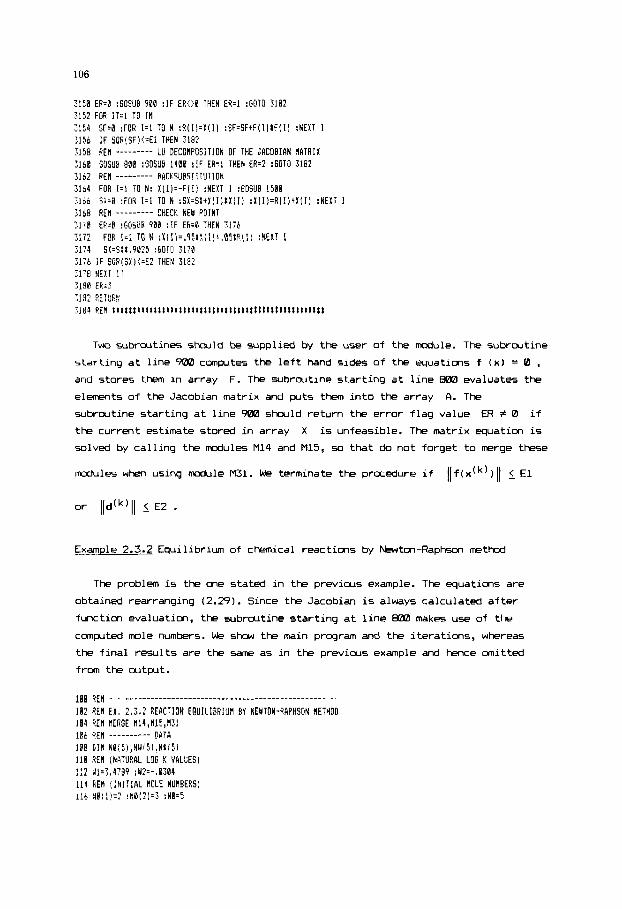
106

3 1 5 9 ER.2 :GOSUB 9 9 0 :IF E R I E THEN ER.1 :GOTO 3182 3152 FOR IT=1 TO I N 3 5 4 SF.0 :FOR 1.1 T O 14 :R(II=X(I) :SF=SFtF(I)tF(II :NEXT I 5 1 5 6 IF SOR!SFJ<=El THEN .?la2 3158 3 6 0 6OSUB 800 :GOSUB 1 4 0 0 :IF E R = I THEN ER=2 :60TO 3162 3162 REW --------- EPCKSURSTITUTION 31b4 FOR 1.1 TO N: X[I)=-F(I! :NEXT I :60SUB 1500 516b 34 : i D R 1.1 TO ti :SX=SXtX(I)fX(I) :XlI!=R(l)tX(!! :NE%T I

317P EP=C :GGSUE WR : I F ER:R THEN 3176 3 1 7 7 3 1 7 4 SX=S(t,90?S :SOTO I170 3 7 6 I i SQR(SX):=E? THEN 3 1 8 2 31’5 t!EXT I T >Id3 ER:3

REN --------- LU DECOWFOSITION OF THE JACOBIRH M T R I X

CHECK NEH POINT 3168 REM _ _ _ _ _ _ _ _ _

FOR 1=1 TO bl : ~ l I ~ = . ? S t X ( l ) t , ~ 5 t R ( ! ~ :NEXT I

7 -

;13? RETURM 3184 RE! r t t t t t t t t t t t t t t t t t t ) t l t t t t t t t t t t t t t t t t t t [ [ [ [ [ t t : [ [ t

Two subrout ines s h x l d be suppl ied by the u s e r of the module. T h e subrout ine

s t a r t i n g a t l i n e ‘902 computes the l e f t hand s i d e s of t h e equat ions f (XI = 0 , and stores them i n a r ray F. The s u b r w t i n e s t a r t i n g a t l i n e 602 evalua tes t h e

elements o f t h e Jacobian m a t r i x and puts them i n t o the a r r a y A. The

subrout ine s t a r t i n g a t l i n e SCdB should re turn the error f l a g va lue ER # 0 i f

the c u r r e n t estimate s tored i n a r r a y X is unfeasible . The m a t r i x equation is

solved by c a l l i n g t h e modules M14 and M15, 50 that do n o t f o r g e t to merge these

modules when using module M31. We terminate t h e prwredure i f I l f ( x c ( k ) ) l l E l

Example 2.3.2 Equilibrium of chemical reac t ions by Newton-Raphson method

The problem is the one stated i n t h e previous example. The equat ions are

obtained rearranging (2.29). Since the Jacobian is always ca lcu la ted a f t e r

funct ion eva lua t ion , t h e subrout ine s t a r t i n g a t l i n e WUl m a k e s u s e of the

canplted mole numbers. We show t h e main program and t h e i t e r a t i o n s , whereas

the f i n a l r e s u l t s are t h e same as i n t h e previous example and hence o m i t t e d

f r m the outplt.

107

2.3.3 Broyden method

The Broyden method is me of the simplest quasi -htan method. The aim of

quasi Newton methods is t n achieve cmvergence properties canparable to those

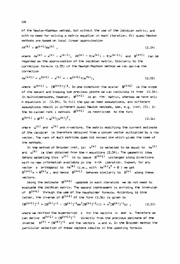
108

of the Newton-Raphscn method, but without the use of the Jacobian matrix, and

with no need for solving a matrix equation in each iteration. A11 quasi-Newton

methods are based on local linear approximation

(2.34)

where ax(k) = , (k) - . (k - l ) , A f ( k ) = f c x ( k ) ) - f ( . ( k - l ) ) and B ( k + l ) can be

regarded as the approximation of the Jacobian matrix. Similarly to the

correction forrmla (2.33) of the Newton-Raphm method we can derive the

correc tion

(2.351

where H(k+l) = [B(k+l)l-l. In me dimension the scalar dk+l) is the slope of the secant and knowing two previous pints we can calculate it from (2.34).

In mltidimensions, however, dk+') is an nXn matrix, whereas we have only

n equations in (2.34). To fill the gap we need assumptions, and different

assumptions result in different quasi-Newton methods, see, e . g . (ref. 15). In

the so called rank 1 methods dk+l) is restricted to the form

where u ( ~ ) and

of the Jacobian is therefore obtained from a colurm vector n-ultiplied by a row

vector. The rank of such matrices does not exceed one which gives the name of

the methods.

v ( ~ ) are n-vectors. The matrix modifying the current estimate

In the method of Broydm (ref. 16) vtk) is selected to be equal to Ax(k)

and u ( ~ )

behind selecting this v ( ~ ) is to leave dk+l) unchanged along directions with no new information available in the k-th iteration. Indeed, for any

vector z orthogonal to (i.e., with A x ( ~ ) z ~ = 0 ) w e get

d k + ' ) z = , and hence dk+l) behaves similarly to along these

vectors.

is then obtained from the n equations (2.34). The gwmetric idea

Using the estimate dk+l) updated in each iteration we do not need to

evaluate the Jacobian matrix. The second improvement is avoiding the inversion of dk+l) latter, the inverse of dk+l) of the form (2.36) is given by [ B ( k + l ) i - l = [~(k)l-1 - CB(~)I-~,TCB(~)I-~,(~ + vTrg(k)~-lu) ,

through the u5e of the Hausholder forn-ula. kcording to this

(2.37)

where we omitted the superscript k for the vectors u and v. Therefore we

can derive H(k+l) = CB(k+l)l-l

inverse H(k) = and the vectors u and v. In the Broyden m e t W the

particular selection of these vectors results in the updating forwla

directly frm the previms estimate of the

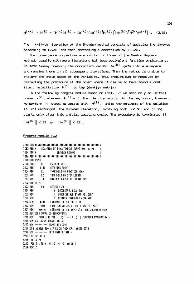
109

The (k+l)- th i terat ion of the Broyden method consists of updating the inverse

according to (2.38) and then performing a correction by (2.35).

The convergence properties are s imi lar t o those of the Newton-Rapkan

method, usually with m r e i terat ions but less equivalent function evaluations.

I n cases, m v e r , the correction vector AX(^) gets i n t o a subspace

and remains there i n a l l subsequent iterations. Then the method i s unable t o

explore the whole space of the variables. This problem can be resolved by

restarting the procedure a t the point where i t claims t o have found a rmt

(i.e., r e i n i t i a l i z e H(') t o the ident i ty matrix).

I n the following program module based on ( ref . 17) w e need only an i n i t i a l

guess

we perform n steps t o update only H(' ) , while the estimate of the solution

i s l e f t unchanged. The Broyden i terat ion, involving both (2.38) and (2.35)

star ts only af ter t h i s i n i t i a l updating cycle. The procedure i s terminated i f

x ( O ) , whereas H(') = I , the ident i ty m a t r i x . A t the beginning, hDwever,

Proqram module M32

32e0 HEM t : t t t t l l t t ;~~l~~~l l t~ l l t ; ;11111:t t t~t :11t :&;;11111~ 3202 HEN I SOLUTION OF SIHULTANEOUS EQUATIONS F(X)=0 t 3204 REtl t BROYBEN METHOP 1 3206 REN ~ t t t t ~ l ~ ~ l ~ ~ t t t t l l l t l 1 t 1 1 ~ & t t t t ~ t t l 1 ~ 1 ~ l 1 1 1 ~ l t 1 ~ & & ~ 3288 REII INPUT: 3 2 1 0 REV N PROBLEN S I Z E 3 2 2 REH ! IN) STARTING POINT 3214 REV E l THRESHOLP ON FUNCTION NORN 3 2 1 6 RE\ E 2 THRESHOLD ON STEP LENGTH

3220 REM OUTPUT: 3222 RE! ER STATUS FLAG 3224 REM 0 SUCCESSFUL SOLUTION 3226 REH 1 UNADHISSIBLE STARTING POINT 1 2 2 8 REM 2 NEITHER THRESHOLP ATTAINED 32Z0 REN $IN) ESTIIIATE OF THE SOLUTION 3232 REII FIN) FUNCTION VALUES AT THE F I N A L ESTIHATE 3234 REH 3236 REM USER-SUPPLIED SUBROUTINE: $238 REV FROH L I N E 9 0 0 ; X [ . ) --> FI.1 [ FUNCTION EVALUATION ) 3240 REH AUXILIARY ARRAY: R(3,N) 3242 RE# ---------- STAPTING POINT 3244 ER.0 :GOSUB 900 :IF ERO.0 THEN ER.1 :GOTO X 4 3246 RER ---------- U N I T MATRIX INTO H

ma REH IN t i~ i~nun NUNBER OF ITERATIONS

H I N , N l ESTIMATE OF THE INVERSE OF THE JACOB1 MATRIX

3248 FOR 151 TO N

3252 FOR J = l TO N : H [ I + J j = - [ I = J ) :NEXT J 3254 NEXT I

3250 RlI,Ij=H

110

1!5a SEF1 ---------- N STEPS TO I N I T I A L I Z E H 2 5 8 FOR t:l TO N : R i l , l ) = 1 0 8 t E ? :60SciB 3292 :R(l,K)=0 :NEXT K 3260 HEN ---------- ITERRTIOM 17 -5~5; I FOR IT=l TO IN 3263 FOR I=: TC I 2 6 6 Sd.0 3268 3270 R!i,I!-SP 3272 NEYT I 2 7 4 M S U B 3292

FOR J.1 TO N :SA=Si ) -H i I ,J ) tF (J ) :NEXT J

3 2 7 4 SA=a :Sr+e 5 x 8 FOR 1.1 T'J H 128P E;;I=SAt;[ I itF(1) :SB=SB+RiI, I )lR(l,I) 3282 NEXT I 3284 RE! --------- CONVERGENCE :?Eb IF SCR(SA)<=E! OR SRR(SB)(=E? THEN EH=A :GOTO 3334 3288 NEXT IT 3 3 0 ER.2 :GOTO 3334 329:' REtl ---------- STEP OF THE BROYDEN flETHOD 3294 FOR 1.1 TO N :X(I)=X[I)+R(l,l) : R l 3 , l ) = F i l ) :NEXT I 3296 ER.8 :EOSUS 9 A I :IF ER.0 THEN 3302 J298 FOR I:1 TO N : X I I ) = X ( I ) - . A 5 1 R i l , I ) :R(I,1)=.95tR~I,I) :NEXT I 3388 6010 32P6 3382 3 3 4 SA=t 3316 FOB 1=1 TO N :308 SB.0 331R 3 1 2 3315 NEIT I 3316 IF SG.0 THEN 3330 3316 FOR J = I TO N 3 2 1 56.0

3324 SB=SB/SG 3326 3328 NEXT J 3336 RETURN 1312 REH ---------- END OF STEP :334 RETURN 3336 RE! l t t t t t t l t l l t l t t t l t t t t t t t t t t t t t l t l l t l t t l l l l t t t t t l t l t ~ ~

FOii l:1 TO N :R(2,I)=F(I)-F(S,I) :NEXT I

FOR J=I TO N : S B = S B t H ( I , J ) t R ( 2 , J ) :NEXT J R ( 3, I )=SB-R( I , I ) :SA=SA+SBtP(I, I )

777-3 FOB I=! TO N :SH=SB+R!I,I)tH(I,J) :NEXT I

FOR 1.1 TO N :H(I,J).H(I,J)-SBtR(a,I) :NETT I

7 -

We need on ly a single user subroutine starting at line 900, which is completely

analogous to the corresponding one required by the Newtm-Raphscn method.

Example 2.3.3 Equilibrium of reactions by Broydm method

In order to complte the reaction equilibrium studied in the previws

examples we slightly change the main program of Example 2.3.2. Lines WMD-810

are omitted and the following lines are replaced:

104 REH HERGE H32

21: LPRIKT 'RROYDEN RETHOD" :LPRlMl

214 GOSUB 3200

111

The part of the out@ that shows the iterations is as follows.

BHOYDEN HETHOD

Table 2.8 shows the computational efforts required to solve the test problem

on reaction equilibrium by five different methods. For cunparison successive

approximation and damped ~lccessive approximation with a damping factor

c = 0.75 are also included.

Table 2.8 Computational effort in different methods

Method kmber of iterations Munber of equivalent function evaluations

Successive approximation 24 24 Damped iteration (c = 0.75) 9 9 Wegstein 11 11

Broyden 9 11 Newton-Rapkon 5 15

____________I____111____________________

Exercises

0 Derive the formlas (2.23) and (2.24) of the Wegstein iteratim from the

0 Consider the n m matrices A and B = A + uvT, where u and v are

gwmetrical idea.

n-vectors and assume that A and B are noneingular..According to the

Hausholder formula, exploited in Section 2.3.3, the inverse of B is given

bY

To prove this relationship, show that B-lB = I . 0 Solve the system Ax - b = 0 with a square, nonsingular A by the Broyden

method and test whether or not the final matrix H will satisfy the equality

H = A-1 .

112

2.4 MINIMIZATIW IN MULTIDIEENSIONS

In this section we deal with the problem of finding the minimum of a

function of more than m e variables.

There are three major families of algorithms for minimization:

i) direct search methods, involving the evaluation of the function f ( x ) only;

ii) gradient methods, based on the use of the gradimt vector g of

the elements gi = af(xl/axi , in addition to the values of f(x);

iii) Newton type methods that require also the Hessian matrix H of the

elements

values.

[HI.. = Sf/axiaxj , in addition to the gradient and function 1J

The direct methods are not very efficient in term of the number of function

evaluations, but are robust, decreasing the objective function up to sane

extent in most cases. Requiring only one user supplied subroutine they are easy

to use.

The most traditional and simplest gradient method is the steepest descent.

Its idea is moving the current estimate x ( ~ ) to the next one x ( ~ + ' ) by

minimizing the objective function along the line from

the local negative gradient

one dimensional minimization problem

x ( ~ ) in the direction of

[ - g ( ~ ( ~ ) ) ] . Thus in each iteration we solve the

(2.39)

called directional search. The entire step is then repeated from the new

estimate as many times as needed. Though the method will decrease the function

value in each iteration, it will perform very m a l l steps in rest cases,

particularly when going down a long, narrow valley. The convergence is of order

1, and the numerical efficiency is poor because of the effort required in the

directional search. Though there are considerably improved versions, e . g . , the

conjugate gradient methods, we will not consider them here.

TIW Newton method will set the next estimate x ( ~ + ' ) to the minimum point

of the local quadratic approximation of the function. Comparing (2.40) and

(2.33)

minimization and for solving a set of nonlinear equations. In (2.401, however,

the matrix H is always symmetric, and at convergmce (but not necessarily in

intermediate iterations) it is positive'definite. The properties of the method

are also retained. The convergence is of order 2, and hence is rapid near the

minimum point, but may be poor far from the solution. In addition, the number

of equivalmt function evaluations is high because of the need for evaluating

H . The Newton method finds, however, the minimum of a positive definite

shows that we use essentially the same correction formula for function

113

quadratic function in a single step, and w e will exploit this advantagwus

property in parameter estimation.

he quasi-Newton methods estimate the matrix c = ti-1 by updating a

previous guess of C in each iteration using only the gradient vector. These

methods are very close to the quasi-r\lewton methods of solving a system of

nonlinear equaticns. The order of convergence is between 1 and 2 , and the

minim of a positive definite quadratic function is found in a finite number

of steps.

The algorithms using first or second derivatives are somewhat m r e powerful

than those using only function values, but not always enough so as to

compensate for the additional function evaluations. Nevertheless, if y w can

compute the the derivatives select a method that will use them. Therefore, the

Newton method is the best choice if you are able to differentiate the function

twice and and have a gccd initial guess. Replacing the derivative with finite

differences is more controversial. If only the gradient vector is available in

analytic form, the variable metric method due to Davidm, Fletcher and Powell

usually dominates the finite difference version of the Newton method. If ycu do

not have analytic derivatives at all, it is usually better to consider a direct

search. From this latter family we describe here the simplex method due to

Nelder and Mead.

2.4.1 SimDlex method of Nelder and Mead

A simplex is the closed gwmetric figure ccnsisting, in n dimensions, of

n+l vertices and all their interconnecting straight line segments. In two

dimensions a simplex is a triangle, not necessarily a regular one. The search

procedure due to Nelder and Mead (ref.18) is based on selecting a starting

simplex represented by n+l vertices x(1), ~(21, . . . , x(~+') and then

successively improving it.

To describe the method w e introduce the following concepts.

n i=l ,

Notice that the centroid excludes the worst point. In one step of the search

the following candidates are investigated in order to replace the worst point:

114

r e f l e c t i o n p o i n t x* = ZP - x(MX)

expansion p o i n t xf* = xf + ( P - x ( ~ ~ ) )

c o n t r a c t i o n p o i n t x*** = ( x ( ~ x ) + ii)/2 .

I f none of these c a n d i d a t e s is better than the worst p o i n t , the s i z e of the

simplex is reduced leaving on ly the bes t p o i n t i n place:

Fig. 2.12 skws the i n i t i a l simplex and the c a n d i d a t e p o i n t s i n two

dimensions. The method is sumnarized i n the logic diagram based on ( r e f . 19)

and shown i n Fig. 2.13.

Fig . 2.12. A simplex i n two dimensions

The iteration is stopped i f the norm of the correction i n the c e n t r o i d and

the d i s t a n c e bet- the bes t p o i n t and the c e n t r o i d are both less than a small

th re sho ld EP . The a lgo r i thm has g r e a t v e r s a t i l i t y to adopt the simplex to the local

landscape of the func t ion s u r f a c e . I t w i l l elongate and t a k e a l a r g e s t e p i f

can do so, it w i l l change d i r e c t i o n on encounter ing a v a l l e y a t an a n g l e and it

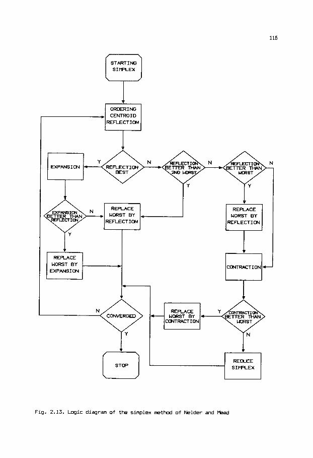
115

STARTING S I M T E X ?

REFLECTION

EXPANSION c I

1 WORST BY

EXPANSION

l-

[2-]

ENTRACTION t Lrl c - SI rPLEX

Fig. 2.13. L o g i c diagram of the simplex method of Nelder and Mead

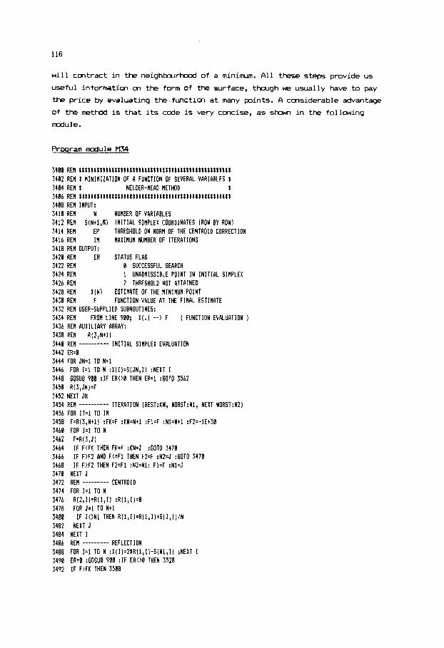
116

w i l l contract i n the neighbourhood of a m i n i m . A l l these steps provide us

useful information on the form of the surface, though we usually have to pay

the price by evaluating the-function a t many points. A considerable advantage

of the method is that i t s code i s very concise, as shown i n the following

module.

Proqram module M34

3480 REM t t t t t t ~ t ~ t ~ t t t t t t t t t ~ t t t l t t t ~ l t t l t ~ t t t ~ ~ t l t l l t l l t t l 3482 REH t MINlHlZATlON OF B FUNCTION OF SEVERAL VARIABLES t 34N4 REM I NELDER-READ RETHOD t

3408 RER INPUT: 3418 RER N NUHBER OF VARIABLES 3412 REH S(Nt1,N) INITIAL SIMPLEX COORDINATES (ROY BY ROW) 3414 REIl EP THRESHOLD ON NORM OF THE CENTROID CDRRECTION 3416 REM It4 M A X I M M I NUHBER OF ITERATIONS 3418 REM OUTPUI: 3428 REH ER STBTUS FLAG 3422 HEM @ SUCCESSFUL SEARCH 3424 REH 1 UNADHISSIBLE POINT I N INITIAL SINPLEX 3426 REH 2 THRESHOLD NOT ATTRINED 3428 REH X(N1 ESTIMATE OF THE HINIMUM POINT 3430 REM F FUNCTION VALUE AT THE FINAL ESTINITE 3432 HEM USER-SUPPLIED SUBROUTINES:

s4ab REM t t t t t t t t t t t t t t t t t : t t t ; t ; t ; t t : : t t t t t t t t t t ~ : t t : t ~ t : t t

3434 RE\ FROH LINE 9 ~ a ; x(.) --> F ( FUNCTION EVALUATION 1 3436 REM AUXILIflRV BRRAV: 3438 REH R(3,Ntl) 3441 RE[ ______---- INITIAL SIMPLEX EVALUITION 3442 ER.8 3444 FOR JN=l TO Mtl 3446 FOR 1=1 TO N :X(I)=S(JN,Il :NEXT I 3448 GOSUB 9BB :IF ERO8 THEN ER=l :60TO 3562 3458 R(S,JN)=F 3452 NEXT JN 3454 REM ______---- ITERATION (BEST:KN, WORST:Nl, NEXT W0RST:NZ) 34S6 FOR 11.1 TO IM 3458 F=R(3,Ntl) :FK=F :KN=Ntl :Fl=F :NI=Ntl :F2=-lEt30 s46a FOR J=I TO N 3462 F=R(3,J) 3464 I F FiFK THEN FK=F :KN=J :60TO 3478 3466 I F F)F2 BHD F(=FI THEN F2.F :NZ=J :GOTO 3478 3468 IF F)F2 THEN F2:Fl :N2=N1: Fl=F :Nl=J 3478 NEXT J 3472 REH --------- CENTROID 3474 FOR 1=1 TO N 3476 R(Z,I)=R(l,l) :R[I,l 1 4 3478 FOR J= l TO Ntl 3480 IF J O N 1 THEN R(1,1l=R(l,l)tS(J,I)/N 3482 NEXT J 3484 NEXT I 3486 REN --------- REFLECTION 3488 FOR 1.1 TO N :X(I~=21R~1,II-S~NllII :NEXT 1 3490 ER.0 :GOSUB 900 :IF E R O B THEN 3528 3492 IF F)FK THEN 3508

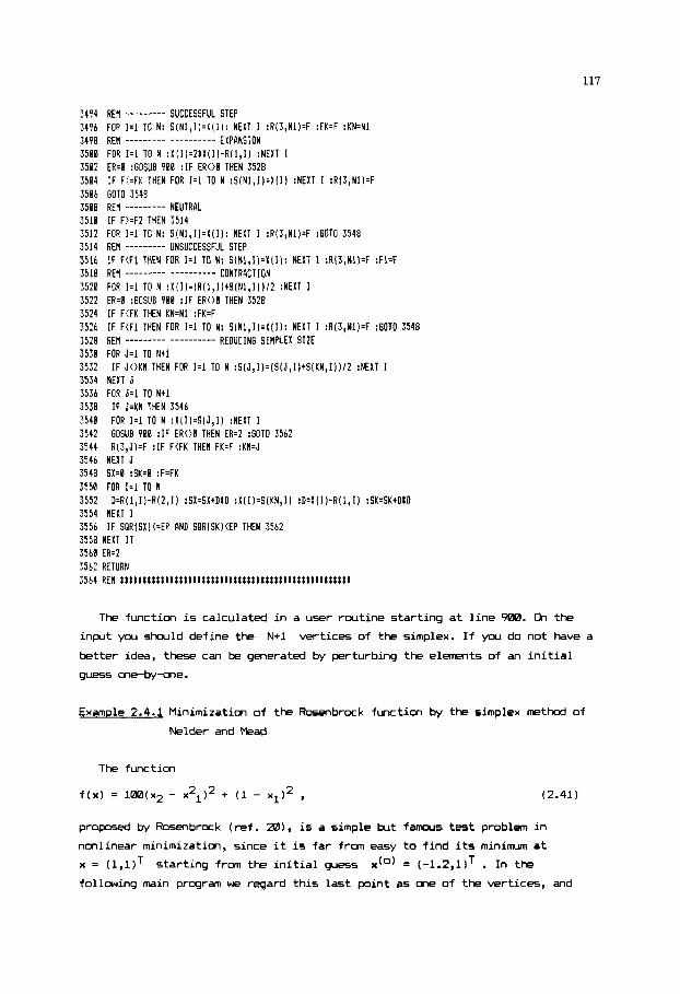
117

SUCCESSFUL STEP 3494 REH _____L- -_

3496 FOR 1.1 TO N: S(Nl,I)=X(I): NEXT I :R(j,Nl)=F :FK=F :KN=Nl

3580 FOR I:1 TO N :XiI)=2tY(I)-R(llI) :NEXT I 3502 ER.0 :GOSUB 900 :IF E R M THEN 3528 3504 IF F(=FK THEN FOR 1=1 TO N :S(Nl,I)=X(l) :NEXT I :R(3,Nl)=F 3505 GOT0 3548 3508 REH --------- NEUTRAL 351% IF F)=F2 THEN 3514 3512 FOR 1.1 TO N: S(Nl,I)=X(I): NEXT I :R(3,Nl)=F :60TO 3548 3515 REH --------- UNSUCCESSFUL STEP 3515 IF F(F1 THEN FOR 1.1 TO N: S(Nl,I)=X(I): NEWT 1 :RIJ,Nl)=F :Fl=F 3518 HEW --------- ---------- CONTRACTION 3520 FOR I=1 TO N :X(I)=IR(l,IltS(Nl,I))/2 :NEXT I 3522 ER=0 :GOSUB 900 :IF ER00 THEN 3528 3524 IF F(FK THEN KN=Nl :FK=F 3526 IF F(F1 THEN FOR 1.1 TO N: S(Nl,I)=X(I): NEXT I :R(3,Hl)=F :6OTO 3548 3528 RE1 --------- ---------- REDUCING SIHPLEX SIZE 3530 FOR J=1 TO Ntl 3532

3498 REn _ _ _ _ _ _ _ _ _ _ _ _ _ _ _ _ _ _ _ EXPANSION

IF J O K N THEN FOR I=1 TO N :S(J,I)=(SlJ,I)tS(KN,1))/2 :NEXT I 3534 NEXT J 3536 FOR J= l TO Ntl 3538 IF J=KN THEN 3546 3540 FOR 1.1 TO N :W(I)=S(J,I) :NEXT I 3512 GOSUB 900 :IF E R 0 0 THEN ER.2 :60TO 3562 3544 R(3,J)=F :IF F G K THEN FK=F :KN=J 3546 NEXT J 3548 SX=E :SK4 :F=FK 3550 FOR 1=1 TO N 3552 D~R(l,I)-RI2,1) :SX=SX+DtD :X(I)=S(KN,I) :D: 3554 NEXT I 3556 IF SORISX)(=EP AND SORISK)(EP THEN 3562 3558 NEXT IT 3560 ER=2 3562 RETURN

I1,I) :SK=SKtDtD

The func t ion is c a l c u l a t e d i n a u s e r r o u t i n e s t a r t i n g a t l i n e 900. l3-1 the

i n p l t you s h w l d d e f i n e the N+1 v e r t i c e s of the simplex. I f you do n o t have a

better idea , these can be generated by per tu rb ing the e l m t s of an i n i t i a l

guess one -byme .

Example 2.4.1 Minimization of the Rosenbrock func t ion by t h e simplex method of

Nelder and Mead

The func t ion

f ( x ) = l0a(XZ - x21)2 + (1 - X 1 P , (2.41)

proposed by Rosenbrock ( r e f . MI), is a s imple b u t famous test problem i n

non l inea r minimization, s i n c e it is f a r frcm easy to f i n d its m i n i m at

x = (1 ,1 )T

fol lowing main program we regard t h i s last p o i n t as one of the v e r t i c e s , and

s t a r t i n g from the i n i t i a l guess x ( 0 ) = (-1.2,1)' . In the

118

generate the other two, perturbing the coordinates of x ( O ) by 0.01 in turn.

100 RE[ ........................................................... 102 REM EX. 2.4.1 ROSENBRDCK PROBLEM BY NELDER-BEAD HETHOD 104 REB MERGE B34 200 REM ---------- PROBLEI SIZE 202 N=2 204 DIH X(N),S(NtI,N),R(3,Ntl) 2Bb RER ---------- CONTROL PARABETERS 208 EP=.08081 :IM=l00 210 RE1 ---------- INITIAL SIBPLEX 212 X!1)=-1.2 :!(2)=.1 214 FOR J = 1 TO Ntl 216 FOR 1.1 TO N 218 220 NEXT I 222 NEXT J 224 VVSTRINH (60, "-') 226 LPRINT 'SIHPLEX METHOD OF NELDER AND HEAD" :LFRINT 228 LPRINT V1 238 GOSUB 3400 232 LPRlNT :LPRINT 'MINIHUM"; 231 LPRINT TAB( 10) ; ' x ( 1 236 LPRINT :LPRINT V$ :LPRINT 258 STOP 900 REM ---------- FUNCTION EVALUATION 902 F:l008 (W!2)-X( 1)*2)^2t( 1-1 (1) )"Z 904 LPRINT USING"IT=l## x 11 l=ll.#lll###A'A* x (2)=11. #####V"* ";IT, X (1) , X (2) ; 906 LPRINT USING'F=#.#####'"*A";F 908 RETURN

S ( J I )=XI I )-.el1 ( 1 4 )

; X ( 1 ) ;TAB(25) ; " Y (2 )=" ; X [ 2) ;TAB( 40) ; " F = O ;F

The shortened iteration history i s as follows.

SIHPLEX IETHOD OF NELDER AND READ

IT= 0 x(l I = - , 1190EEE+B1 Y (7)4.lEllEE0Et0E F=E. 17BBlEt03 I T = 0 x(l)=-. 120000Et01 ~(2)=B.l10000Et00 F4.18173Et03 IT= B x(l I = - , 12000BEt01 x [ 2)=0.10B000EtBB F=8,1844BEt03 IT= 1 r ( 1)~-.119000Et01 x[2)=0.110000E+00 F=0. 17539Et03 IT= 1 x(I):-.118500Et01 x(2)=0.115000Et00 F4.17098Et03

11. 50 ~(1)=0.975553EtBB x(?)=B,9426%E+B0 F=0.87133E-82 IT= 51 x (1 )4.101253Et01 x (2)=0.1014%3EtBl F d . 10619E-01 I T = 51 x (1 )=8.98SB04Et00 x (2)=0.963877Et00 F4.42642E-02

IT= 83 xll)4.999987Et00 x(2)=0.999977Et00 F=0.67?69E-09 IT. 83 ~(1)=8.999998E+BB ~(2)=8.999995Et00 F.8.55511E-10 IT= 84 x (1 )4.lB000lEt01 x 12 )=0.100002Et61 F=0.88448E-10 IT= 84 x ( 114.1000BBEt01 x (2)=8.10000lEt01 F=0.33879E-10 IT= 85 x [l)=@. 1000@BEt01 x (2)=0.lB000BEt01 F4.53944E-10

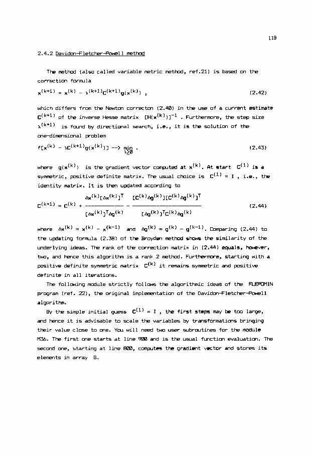
119

2.4.2 Davidonfletcher-Powell method

The method (also called variable metric method, ref.21) is based on the

correction formula

x ( k + l l = .(k) - x ( k + l ) C ( k + l ) g ( x ( k ) ) (2.42)

which differs from the Newto, correcton (2.40) in the use of a current estimate

C(k+l) of the inverse Hesse matrix [ H ( x ( ~ ) ) ] - ' . Furthermore, the step size is found by directional search, i.e., it is the solution of the

one-dimensimal problem

f [ x ( k ) - ~ ~ ( k + l ) g ( x ( k ) ) ~ --> min . (2.43) A20

where Ax(k) = - x(k-l) and Ag(k) = g ( k ) - g(k-l). -paring (2.44) to

the updating formula (2.38) of the Broydm method shows the similarity of the

underlying ideas. The rank of the correction matrix in (2.44) equals, however,

two, and hence this algorithm is a rank 2 method. Furthermore, starting with a

positive definite symmetric matrix

definite in all iterations.

d k ) it remains symmetric and positive

The following module strictly follows the algorithmic ideas of the n r W M I N

program (ref. 22) , the original implementation of the Davidmfletcher-Powell

algori t h . a/ the simple initial guess 191) = I , the first steps may be t w large,

and hence it is advisable to scale the variables ty transformations bringing

their value close to one. You will need two user subrcutines for the module

MJ6. The first one starts at line Sew and is the usual function evaluation. The

second me, starting at line tMa , cmputes the gradient vRtor and stores its

elements in array G.

where g ( ~ ( ~ ) ) is the gradient vector computed at xCk). At start dl) is a symmetric, positive definite matrix. The usual choice is

identity matrix. It is then updated according to

dl) = I , i.e., the

120

Proqram module M36

3688 RE! t t t t t t t t t t t t t t t t t t t t t t t t l t t t t t t t l t t t t l t t t t t t t t t l t t t 3682 REM t M I N I M I Z A T I O N OF A FUNCTION OF SEVERAL VARIABLES t 3684 REH t DAVIDON-FLETCHER-POWELL HETHOD t 3686 R E 1 t t t t t t t t t t t t t t t t t t t t t t t t t t t t t t t t t t t t t t t t t t t t t t t t t t t 3688 REM INPUT: 3610 REH N NUMBER OF VARIABLES 3612 REN XIN) STARTING POINT 3614 RE\ EF THRESHOLD ON STEP LENGTH 3616 REM IH HAXIHUH NUMBER OF ITERATIONS

3620 REH ER STATUS FLAG 3622 RER B SUCCESSFUL SEARCH 3624 REW 1 UNADHlSSlBLE STARTING POINT 3626 RE! 2 ESTIHATE C IS NOT P O S I T I V E D E F I N I T E 3628 REH 3 UNIDIRECTIONAL SEARCH F A I L E D 3638 REM 4 THRESHOLD NOT ATTAINED 3632 REH K I N ) ESTIHATE OF THE MINIHUH POINT 3634 REH F FUNCTION VALUE AT THE F I N A L ESTIHATE 3636 RE# G ( N ) GRADIENT VECTOR AT THE F I N A L ESTIHATE 3638 REM C[N,N) E S T I H I T E OF THE INVERSE HESSIAN i l A T R l X 3648 REH USER-SUPPLIED SUBROUTINES: 3642 REH FROM L I N E 988; XI.) --> F ( FUNCTION EVdLUBTION ) 3644 REM 3546 REH AUXILIARY ARRRY: 3648 REI! R(3,N) 3650 ER=B :GOSUB 900 : IF E R O B THEN ER.1 :GOTO 3792 3652 GOSUB 8BB 3654 REN ---------- I N I T I A L I Z E C TO U N I T MATRIX 3656 FOR 1.1 TO N 3658 FOR J = l TO N :ClI,J)=-lI=J) :NEXT J 3660 NEXT I 3662 RE# ---------- STPRT OF ITERRTION 3664 51.1 3 6 6 6 FOR 11.1 TO I N 3668 GB=8 :GA=B 3 6 7 0 FOR 1.1 TO N 3672 Rl2, I )=I I I :Rl3, I ) 4 1 I ) : R 4 3 6 7 4 FOR J.1 TO N : R = R - C I I , J ) t G I J ) :NEXT J :R[l,I)=R 3676 GB=GBtG( I ) tR : G A = 6 A t G ( I ) t G [ I ) 3678 NEXT I

3618 REI~ OUTPUT:

FROH L I N E 888; XI.) --> 6(.) 1 GRADIENT VECTOR EVALUATION )

3 ~ 8 FO=F :IF GA=B THEN ER=B :GOTO 3792 3682 REH ---------- DIRECTIONAL SEARCH ALONG s

3688 SP=ST

3684 FB=F 3686 IF GB)B THEN ER.2 :GOT0 3792

3698 REN _ _ _ _ _ _ _ _ _ _ ______________- EXTRAPOLATE

3692 FA=FB :GA=GB 3694 FOR 1.1 T O N : X I I ) = X ( I ) t S P t R ( I , I ) :NEXT 1 3695 ER=B :GOSUB 988 :IF ER=B THEN 3 7 8 2 5698 FOR 1.1 TO N : X ( I ) = X I I ) - S P t R l I , I ) : R l l , l ) = . 9 5 t R ~ l , I ) :NEXT I 3788 GOT0 3694

3784 FP=F :GB=B 3 7 8 6 FOR 1.1 T O N : G B = G B t G I I ) t R l l , l ) :NEWT I 3788 I F 6K8 AND F K F A THEN SPz4ISp :ST=4tST :GOTO 3684

3 7 8 2 GOSUP 888

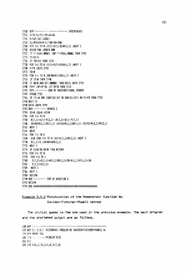
121

REfl ._________ ___.___________ INTERPOLATE

2.31 (FA-FP) 'SF'tGPtGB W=SW (Zt Z-GAtGP! S L 4 F t ( G B + W - Z ) / IGB-GPtZtW) FOP I=l TO N :YIII=X(I)-SLtR(I,I) :NEXT I 502% 780 :GOSUB 800 IF F(=FPtl.BBB01 AND F<=FBtl.EBBEl THEN 3742 ST=ST/4 IF FR)=FP THEN 3732 FOR I = I TO N :XlI~=~lI)~SLtR(l~I) :NEXT I F=FB :GOTO 3742 GR=0 FOR 1.1 TO N :GB=GB~G(1)tR(l,I) :NEXT I IF IT<N THEN 3740 IF GB(8 AND ST(.BBBBBl THEN ER=3: 6010 3792 FB=F :SP=SP-SL :IF SP>0 THEN 3712 REn _____--__- END OF UNIDIRECTIONAL SEARCH GOSUB 3752 IF ITi=N AND (SOR(SS)IEP OR SQR[SI)(EPl OR F M O THEN 3792

3748 NEXT IT 3750 ER.4 :6DTO 3792 3752 REH ---------- UPDATE C 3754 3756

3768 37 b2 3764 3766 3768 3770 3772 3774 3776 3778 3786 3782 3784 3786 3788

3758

SG.0 :SS:0 :SI=B FOR 1.1 TO N R(?,I)=X(II-R(2,1) :R(3,1)=6(I]-R(3,1) SG=SG+R(2, I ) t R ( Z , 11 :SS=SS+R( 1 , I ) I R ( 1 I I I :SI=SItR(Z, I I lR(2, I1

NEXT I GH.8 FOR 1.1 TO N 5.0 :FOR J.1 TO N :S=StC(I,J)tR(S,J) :NEXT J R(l , I ) = S :GH=GH+StR(3, I ]

NEXT I IF 56.8 OR 6H=0 THEN RETURN FOR I=1 TO N

FOR J=l TO I C( I, J ) z C ( I, J )+R(Z,I) tR(2, J)/SG-R( 1,I 1 lRll I Jl/GH C( J , I )=C( I ,J

NEXT J NEXT 1 RETURN

3798 REH ---------- END OF UPDPTING C 3792 RETURN 3794 REH t t t t t t l l t t t t l t t t t t l l t t t I t t t t t t I t t It I l l t t tt ttt t t t t l t

Example 2.4.2 Minimizatim of the Rosenbrock function by

Davidonfletcher-f'cwell method

The i n i t i a l guess i s the me used i n the previous example. The main program

and the shortened artput are as follows.

122

?US REM ---------- CONTROL PARMETERS ,@L iP=.00001 ;ItI=l00 218 REF ---------- INITIAL POINT ::2 X(1)=-1.2 :X[2]=,1 214 V$=STRING$[CB,'-"] 216 LPRINT 'DPVIDON-FLETCHER-POWELL METHOD" :LPRINT 218 LPRIlT V1 228 SOSUP 5688 222 LPRINT :LPRINT 'IfINlHUM'; 224 LPRINT TAR( 181 ; " x 11 I='; X I1 ! ; TAB1251 ; ' x (2 )=" ;X I21 ;TAB()#! ; 'F=';F 226 LPRINT :LPRINT V$ :LPRINT 228 IF E R O B THEN LPRINT 'STATUS FLA6:';ER 238 STOP 810 REM ---------- GRADIENT EVPLUlTION 882 GI 11~-48011X121-Xll)A2)t1 (1 l-21( 1-1 (11 I 804 612). ?UBt(X(2)-X(1)̂ 2) 886 RETURN 9e0 REW ---------- FUNCTION EVALUATIDN 902 F=llBtlW(2)-X[ 1 )"2)"2+( 1-1 (1 11'2 904 LPRINT USING'IT=### x (ll=#.##WAA** ~121=#.1##111~*~" "; IT.K( 1 I tX121 ; 986 LPRINT USIN6"F=#.##l##A*AA";F 988 RETURN

DAVIDON-FLETCHER-POWELL IETHOD

............................................................ I T = 0 x I1 l=-.12BUBEt81 x 121=0.1BB00EtB0 F=B.l8440Et03 I T = 1 ~(11-0.64648E+U3 x(2)=0,2681BEtU3 F-8.17436Etl4 IT= 1 x111=0.2156%E~03 xl21=0.8?821EtU2 F=8.21525Et12 11. 1 x (1 I=0.72EB2Et82 x I2 1 =0.383?3Et82 F=ES2656?Et18 IT= 1 XI 11=U,24126E+82 xl2)=8.10581EtB2 F=8,32662Et88 IT= 1 XI 11=8.91463EtBl P (2]=8.3?678Et~l F=0,38?35Et06 IT= 1 x i 1 14.27649EtUl Y [2]=0.174U8EtRl F=8,34887EtB4 IT= 1 x ( 1 I =On 82338EtB0 x ( 2 I =0, 93735Et08 F=0,67596Et81 IT= 2 x (1 1=0.86586E+B0 x12)=8.86315EtBE F=B. 13848EtU1 IT= 2 x i 11=0.18358EtUl x121=U.56633EtUB F4.25653EtU2 IT= 2 :: I1 1=0.89828EtBB x(2)=0.88658Et00 F4.18364E-81

IT= 12 ~Il14.97897Et80 x(2]=B.?66?2Et8B F=U.!7?53E-b)2 IT: 12 x I 11:8.99?73EtU0 x(2)=8.?9?46EtBB F=0.75?76E-U7 IT= 13 ~IlI~R.10139Et81 ~(21=8. 102BBEt81 F4.19362E-03 IT= 13 x i 1 I=U.l0U8UE+01 x [2!=8.lUU80Et8l F=0.28422E-10 IT= 14 i: (1 1=8.97970E+UE x l2)=0.??93?Et80 F4.11266E-86 IT. 14 x(l 1=8.10008E+01 x(?)=0.1088UEtBl F=8.8U00BEt08

#INIHUH x(ll= 1 x(2l= 1 F= 0

The method needed 44 function evaluations, almost four tims less than the

simplex method of Nelder and Mead.

the equation f'(x) = 0 instead of the m i n i m of a differentiable function

f(x) . This trick rarely gives you any g a d in rmltidimensions. First, as w e

emphasised, solving a system of nonlinear equations is m r e difficult than

We noticed that in me dimension it may be advantageous to seek the r m t of

123

sliding downhill on a single surface in minimization, where you can always

measure your progress. Second, you may bring in several roots that are not

minimum points. These problems raise another question. If solving system of

equations is so hard, why not to replace it by minimization of the function

g = fTf

a global minimum of zero exactly at all solutions of the original set of

equations. Lhfortunately, in multidimensims this trick does rarely work

either. Y o u must be prepared to have several local minima of the function g ,

and each local minimum is a trap for the minimization teclniques. Therefore

equation solving and minimization are completely different problems in

rmltidimmsions, in spite of their algorithic similarities.

in all cases? Indeed, the function g is positive semidefinite, and has

Exercises

Solve the problem in Example 2.3.1 by minimization.

0 Find the minimum of the R-brock function by solving the nonlinear

equations df(x)/h = 0 .

0 Find the m i n i m of the quadratic function

f(x) = (1/2)(x - bITA(x - b)

by the Davidon-Fletcher-Pcwell method selecting A to be an n m symmetric,

diagonally dominant matrix with positive diagonal elements. Check if the

equality C = A-' holds at convergence.

2.5 APPLICATICNS cy\ID FLRTI-ER PROBLEMS

2.5.1 Analvtic solution of the Michaelis-Wenten kinetic eauation

The simplest mechanism of enzyme reactions is of the form

kl k3 --> -->

E + S ES E + P , <-- <-- k2 k4

(2.45)

where E, S , P and ES denote the enzyme, the substrate, the product and the

enzyme-substrate complex, respectively (ref. 23). The reaction rates are

124

(2.46)

where kl, k2, k3 and k4 are the rate coefficients and C.1 denotes

concentration of the corresponding species. 6s we will discuss in Section 5.4,

the quasi steady state approximation

approximation of the global reaction

VsCSI/Ks - VpCPl/Kp r = r1 = r2 =

1 + [S]/Ks + [PI/+

where

Vs = k3CEIo, Vp = k2CE10, KS

for species CES] gives an excellent

rate for nmst enzyme reactions:

(2.47)

are called Michaelis-Menten parameters.

Introducing the reaction extent x = [Slo - CSI = CP] , corresponding to the initial condition [PI, = 0 , equation (2.47) is of the form

(2.48)

where

The differential equation (2.48) is separable, and by integrating the rational

function on its right-hand side the solution is given by

t = D EX + - $1 log [--.--I A + Bx . (2.49)

We want to use (2.49) to calculate the concentration [PI at t = 180 s in the

enzy-atalysed hydrolysis of fumarate, with the initial enzyme concentration

[El, = 5 ~ 1 0 - ~ m l / m 3

Michaelis-llentm parameters for this reaction are

KS = 3.9 m l m-3 , By (2.48) dx/dt = 0 implies A + Bx = 0 , and the equilibrium reaction

coordinate +/B clearly is an upper band on the solution. Use the methods of

Section 2.1 to verify the solution

and substrate concentration [S], = 40 ml/m3. The

Vs = 0.65 mmol m-3 s-’,

Vp = 0.4 m l m-3 5-l and Kp = 10.3 m l

[PI = 32.268 mnol m-’.

125

2.5.2 Solution equilibria

In textbooks of cmptational chemistry y a will invariably find examples

calculating the

acid - weak base solutions. Indeed, these examples are important in the study

of acids, bases and of complex formation, as well as for calculating titration

curves. Following (ref. 24) we consider here the aquas solution that contains

a weak tribasic acid H$ and its sodium salts in knam

initial concentrations. The dissociation reactions and equilibrium relations

are given as follws.

pH = - lg (CH+l/(mol/l)) in weak acid - strong base or strong

w, N a p and Na$

-> K,, = CH+lCU-l-l .

Further constraints are the mass balance equation for the total acid

concentration CA

cA = C ~ I + c y - 3 + "?-I + CA~-I ,

and the charge balance equation

CH'I + "a+] = CH9-I + 2CW2-1 + 3[fi3-] + [M-3 . F r m the initial conditions

and

(2.50)

(2.51)

(2.52)

(2.54)

( 2 . 5 5 )

where the initial concentrations are denotedf by subscript o . To calculate the

hydrogen ion concentration we express

equilibrium relations

and substitute these expressions into (2.54). As a rewrlt we obtain the

expressions

CH91, CH9-I and CW2-1 from the

(2.501, (2.51) and (2 .52) using only CO3-I and CH'I

126

CH3.41 = CH+I%A/D, [v-I = K1[H+I2CA/D,

CHn2-3 = K1K2CH+]CA/D,

where

D = CH+I3 + K1[H+l2 + K1K2[H+l + K1KzK3.

CI-!A'-~ = KIK-$JCFI/D, (2.56)

Substituting (2.56) into the charge balance equation and using (2.53) to

eliminate [W-] we obtain the fith-order polynomial equation in CH+] :

CH+15 + alCH+14 + a2CH+13 + a3CH+12 + a4CH+l + a5 = 0 , where

al = K1 +

a2 = K1(K2 + [*+I - CA) - $

a3 = KlCKz(K3 + CNa'I - X.4) - $1

a4 = K1K2CK3(CNa+l - 3 c ~ ) - $1

(2.57)

a5 =-%K-$3% - We want to calculate the equilibrium pH of the solution if its initial

composition is given by

based logarithms of the dissociation constants are:

lgCK1/(m1/1)1 = -2.15, lgCK2/(ml/l)l = -7.21, lgCK1/(~l/l)l = -12.36

CH,po410 = 1 ml/l and CNa3p0410 = 1 mol/l . The ten

and KV = 10-14 m12 1-' ,

Equation (2.57) has five, real or complex rwts. From chemistry, hOwever, we

k n w a good starting guess for the pH (it is slightly above 71. king this

information we can easily find the solution applying any of the methods of

Section 2.1. For extreme initial concentrations it might be necessary to scale

the variable, e.g., by introducing

special methods for finding all rwts of a polynomial equation, see e.g.,

(ref. 121, but then you shwld "polish" the selected real root for higher

accuracy, e.g., by Newtan+aphson iteration. With the a priori information

available in scientific applications, you rarely need such special methods.

x = 107CH+l . We note that there are

Exercise

It is interesting to try to solve the original system of equations (2.50 - 2.55) in six unknowns using m e of the methods of Section 2.3. The

canpltational effort is certainly higher and yar should select the starting

values of the variables very carefully.

121

2.5.3 Liquid-liquid equilibrium calculation

The determination of the equilibrium composition in two contacting liquid

phases has great significance for extraction process design. To obtain a system

of equations we need a thermodynamic model for the excess Gibbs free energy

&/(RTl . We chose the

the excess Gibbs free energy of a

mole fractions zl, z2, ..., zc :

3-wffix Margules equation (refs. 25-26) expressing

C component liquid as a function of the

L?& c c c c c .?-I T ZkZIZ$*klm (2.58)

Tl T7 -__ - - 2, (Zk)2z1Alk + 2, I, RT k=ll=l k=l l=k+l m=l+l

l#k

where

and the table of coefficients Akl, which can be determined from infinite

dilution activity data, is supposed to be known. The activity coefficient

of the i-th cmpment can be cmpted from the thermodynamic relation 7i

(2.59)

where ni is the mole number of the i-th cmpment, n is the total mole

number and the second equality holds only because

expression of the mole fractims.

(2.58) is a cubic

Let us denote by superscript R the raffinate phase and by superscript E

the extract phase. In equilibrium the distribution ratio can be

calculated from the activity coefficients (or rather from their logaritk) as

zEi/zRi = Ki

K~ = 7Ri/7Ei = exp( log 7Ri - log 7Ei . (2.60)

Equations (2.58-2.60) form the thermodynamic base for liquid equilibrium

calcula tions . Suppose we add 6.6 mol Furfural (1) to the mixture of 0.2 mol n-l-leptane

(2) and 0.8 mol Cyclohexane (3). We want to determine the composition of the

extract phase rich in Furfural and of the raffinate phase poor in Furfural. The

Margules coefficients (ref. 26) are shown in Table 2.9.

128

Table 2.9 Aij coeff ic ients fo r the Furfural -

i\ j 1 2 3

1 3.16992 3.0975 2 3.1252 - 3 2.3399 0

n-Heptane - Cyclohexane system

-I---

- 0 -

We have eight unknms: x1 - the raf f inate i n moles, x2 - the extract i n

moles,

mole f ract ion of n-Heptane i n the raf f inate phase,

Cyclohexane i n the raf f inate phase;

extract phase i n the came order. The eight equations are as follows.

Overall material balance

x3 - the mole f ract ion of Furfural i n the raf f inate phase, x4 - the

x5 - the mole f ract ion of

x6, x7 and x~ - the mole fractions for the

~1 + ~2 - 7.6 = 0 ;

mole f ract ion summation fo r the raf f inate phase

x3 + x4 + x5 - 1 = 0 ;

material balances fo r each component

~ 1 x 3 + x2x6 - 6.6 = 0 ~ 1 x 4 + ~ 2 x 7 - 0.2 = 0 x1x5 + X2X8 - 0.8 = 0 ;

and equilibrium conditions fo r each component

(2.61)

(2.62)

(2.63)

(2.64)

In the f o l l m i n g main prqram equations (2.61-2.64) are solved using the

Broydm method. The d is t r ibut ion coeff ic ients are complted from equations

(2.58 - 2.60) wri t ten for C = 3 components. The s tar t ing values us& are

very simple, f o r the extract phase w e s t a r t f rom poor Furfural and fo r the

raf f inate phase from the or ig inal n-Heptane - Cyclohexane mixture. Negative

mole numbers and mle fractions are not allowed.

100 RE# ........................................................... 102 RE# EX. 2 . 5 . 3 LIQUID-LIOUID EOUILIBRIUH BY BRDYDEN METHOD 104 RE# MERGE ti32 166 RER ---------- DATA 106 REH RARGULES COEFFICIENTS (FURFURAL, N-HEPTAHE, CVCLDHEXRNE) 110 A124 .16B92 :A134.0?75 :P21=3.1252 :P31=2.3393 :A?:=@ :P3?=0 11: A12~=(Al?tA?ltAlStR3lrA23+A32)/2 200 RER ---------- PROBLEn SIZE AND CONTROL PARAflETERS 3 2 N=B :Ifl=38 :El=.000001 :EZ=.00000I 204 D In X (N1 ,F ( N I ,HI N,N 1 ,R ( 3 ,N I

129

206 RER ---------- STARTING VALUES 208 RER RAFFINATE ll4OLl AND EXTRACT IflOL) 218 X!l)=l :X[2)=h.6 212 KEN RAFFINATE ROLE FRACTIONS AND EXTRACT ROLE FRACTIONS 214 Xl$l=8 :X(41=.? :X (5 )= .8 :X[6)=l :X(7)=8 :X(8)=8 216 RER ---------- CALL RODULE 218 V$:STRINGI( 53, "-" 1 220 LPRINT 'BROYDEN RETHOD" :LPRINT 222 GOSUB 3280 224 LPRINT :LPRINT V$ 226 LPRINT ,"RAFFINATE EXTRACT' ?2@ F$= 'HBLES 1.11111 [t1.111%) 1.11111 1#1.#11%)' 238 LPRINT USING F1; XI 1) ! XI l)/lX (1 ItXI? 1 ) tl0B,X(21 , X ( ? ) I ( X 11 ItX(2) 1 I188 234 LPRINT USING FI; 10BtX13),10BtX(6] 236 F)= "N-HEPTANE ##.111% #1,1#1%" 238 LPRINT USING FI; l00If(4),lBBtX17) 240 FI= "CVCLOHEXAN i l # , # I # X #1.#1#%" 242 LPRINT USING F); 108tX(5l,lBB1X(8) 244 LPRINT V I 24h STOP 900 REN ---------- F I X ) 902 E R 4 :FOR IE.1 TO N: ER=ER-lYlIE)!B):NEXT IE :IF E R M THEN RETURN 904 HER DISTRIBUTION COEFFICIENTS FROM LOG ACTIVITY COEFFICIENTS 9Uh Zl=Xl3) :Z?=X(41 :Z3=Xl5) :EOSUB 958 :Kl=Ll :K2=L2 :1(3=L3 908 Zl=116) :ZZ=Xi71 :23=X(8) :GOSUB 950 910 KlzEXPIKl-Lll :K2=EXPIK?-L?) :K3:EXPlK3-L3) 912 REfl EQUATIONS 914 FIlI=X(l!tX[21-7.6 :REM MASS BALANCE 916 F ~ 2 ) ~ X ( 3 ) t X ~ 4 ] t ~ ~ 5 1 - 1 918 F131-X I1 IIX lS)+XlZIlX 161-h.6 :RER FURFURAL MASS BALANCE 920 Fl4l=XIl 1tX (4) +XI21 lX171-.2 :RE# N-HEPTANE HASS BALANCE 922 FI51'X 11) lXl51tX 12IlX 181-.8 :REN CYCLOHEXANE HASS BALANCE 924 Flbl~XIhl-KltXl3l : REH EQUIL I BRI UW 9% F171~X171-K2tX141 :REH " 928 F[8)=X18)-K31X[5) :REH ' 930 LPRINT " IT=n ; IT; TAB1 10) "R=" ; X I1 ) TAB1321 "MOLE FR: ' ; X 13) ; X I 4 1 ; X I51 932 LPRINT TAB(l0) "E=':;X[?)TAB(321" ';X161;X17);X181 934 FOR KF.1 TO 8:LPRINT ,'F('~F")=';FIYF):NEXT KF :LPRINT 938 RETURN 958 HEN ---------- LOG ACTIVITY COEFFICIENTS FROM 3-SUFFII HARGULES EOUATlON 952 DG.2 1'21 I ZZlA21+131ri31 ItZ2'21 I ZllA12tZ3IA32) tZ3'21 1 ZllA13tZ2IA23 1 954 DG=DGtZltZ2tZ3tA123

:RE\ ROLE FRACTION SUHWATION FOR RAFFINATE

956 L1~2121llZ2IA2l~Z3lA~l ltZ2*21A12tZ3*2tA13tZ2123tA123-~lD6 958 L2=2122t( ZllA12~Z31A3~1~Z1'2tA21tZ~A21A2~tZl1131A123-21DG 960 L3~2tZ3l~ZllA13~Z2lA23l~Zl~2lA3ltZ2*2l~32tZllZ2lAlZ3-2lDG 962 RETURN

After 17 iterations we arrive at the equilibrium compositions.

..................................................... RAFFINATE EXTRACT

tlOLES 8.1086h ( 1.324%) 7.49934 (98,h76%) FURFURAL 6.896% 87.915% N-HEPTANE 27.688% 2.295% CYCLOHEXAN 65.41b% 9.7982

Calculation of other types of phase equilibria, e . g . , vapor-liquid

130

equilibrium, are based on similar principles. If the same thermodynamic model

is used for both phases, the method (whatever sophisticated it is) can easily

converge to identical compositions in the two phases. This is called trivial

solution and the best way to avoid it is to start from physically reamable

guesses of the compositions.

2.5.4 Minimization subject to linear wualitv constraints: chemical eauilibrium

comwsition in qas mixtures

If the n variable function f(x) should be minimized subject to the

m < n independent linear constraints

A x = b , (2.65)

where A is a given m m matrix and b is a given m-vector, then the method

of Lagrange multipliers might be useful. We introduce the n+m variable

function

L(x;A) = f(x) + (C\x-bITA , (2.66)

where A is the m-vector of Lagrange rmltipliers. At the constrained minimum

point the Lagrange function has zero partial derivatives with respect to all

its variables, i.e.,

fx(x) + A ' X = 0 , (2.67)

A x - b = 0 , (2.68)

where fx(x) is the gradient vector of the objective function f . The set of

equations (2.67-2.68) is solved by the Newton-Raphson method, linearizing

(2.67) around a feasible initial guess

corrRtions Ax together with the rmltipliers A can be obtained from the

n + m linear equations

fx(xo) + Fx,(xo)Ax + ATA = 0 , (2.69)

clbx=0, (2.70)

xo satisfying (2.68). Then the

where Fxx(xo) is the Hessian matrix of the objective function f complted at

the point xo . The uwal procedure of solving (2.69-2.70) is to add the

corrections Ax to the initial guess x' and repeat the iteration until

convergence. An important property of the algorithm is that any new point

x = xo + W x (2.71)

is also a feasible solutim in the sense of (2.65), whatever the scalar 5 is.

Cansequently, we can make a reduced correction with 5 < 1 , if the calculated correctiqn is not acceptable.

131

Equations (2.69 - 2.70) can be solved by standard LU decomposition and

backward substitution, but very often we can reduce the computational e f f o r t

considerably by making use of the special structure of the equations. I n the

chemical equilibrium problem these ideas lead t o a very concise algorithm.

I f the temperature T and pressure P of a closed system are kept

constant, the to ta l Gibbs free energy i s minimum i n equilibrium. For an ideal

gas mixture of species the Gibbs free energy i s given by NS

NS Ns rl 0

G = L ni[ g.(T) + RT log (P/Pu) + RT log [ ni / n j ] ]

j =1 i = l

where R i s the universal gas constant, ni

i - t h species, g . (T) i s the standard molar

spRies corresponding to temperature T and

discussed i n Section 1.8.1, the mole numbers

constraints

0

1

&I= b ,

(2.72)

i s the number of moles o f the

Gibbs free energy of the i - t h

standard pressure Pu. As

rmst sat is fy the atom conservation

(2.73)

where CI i s the atom matrix with bH rows and NS colwms, and b i s the

bH vector of the i n i t i a l elemental abundances.

Kncwing the standard molar Gibbs free energy values and giving an i n i t i a l

mole number vector the determination of the equilibrium composition cms is t s of

minimizing (2.72) subject t o the l inear constraints (2.73). The d i rec t

appl icat im of (2.69-2.70), hOwever, would be rather complicated. I n the

FWUD method ( re f . 27) a function f(xl,x2,...,x~+1) of Ns + 1 variables i s

minimized instead of the funct im G(nl,nZ, ..., nW) of Ns variables, f

being defined as

where

(2.74)

and the relations between the mole numbers ni and the new variables xi are given by

132

NS

xi = ni, (i = 1, 2, ..., NS) ; XNS+~ = 2: nj . j =1

The m i n i m of (2.72) subject to (2.73) can also be found minimizing

(2.74) subject to an extended set of constraints:

(2.75)

%,1"1 + %,2X2 + ... + aNA,NSXNs = % + x2 + ... + xm - xm+1 = 0.

Due to the simple structure of the function f, its first and second partial

derivatives are easy to cmplte

Cfxli = fi ( i=1,2, ...NS )

Ns

Cfxl&+l = -[ c xj 3 1 x*+1 = -1 j=1

With the above derivatives equations (2.69) are given by

NA

LJ 3 J 1

71

fi + Axi/xi - ) h.a.- - = 0 (i=1,2, ... NS) (2.76) j =1

- AXNS+l/XNS+1 = 0 - (2.77)

From (2.76) and (2.77) the corrections Axl, Ax2, ..., AX^+^ can be

expressed as

NA 7 - 0

Axi = xi(-fi + k+l + 1, xjaji1 , (i=1,2, ... NS) (2.78) j =1

133

(2.79)

Substituting (2.78( and (2.79) into the actual form of (2.70) we obtain

the set of W1 linear equations in W1 unknowns with the coefficient

matrix and right hand side vector as follows.

11 A 2 ... h 1 Right h. s.

The solution of this matrix equation is used to compute the corrections

(2.78-2.79). If the correction vector results in me or more zero or negative

mole numbers, equation (2.71) is applied with 5 selected to give maxim

9SL reduction in any mole number in one iteration step.

Notice that the number NA of a t w is usually -11 compared to the number

Ns of species, and hence the f?MD algorithm is very effective in terms of

compltational effort. The rank of the atom matrix, hawever, must be equal to

the number W of atans. At this point it is interesting to remark that

instead of the atom matrix we can use a virtual atom matrix, i.e., the matrix

of reaction invariant coefficients if the atom matrix is not available or we

are interested in a restricted equilibrium. For details see Section 1.8.1.

The following main program is an implementation of the RAM) algorithm. Its

use is illustrated on the example of hydrazin combustion at

P = 5.17Xl& Pa

T = 35DZl K and

(ref. 27). The elemntal atundances of hydrogen, nitrogen and

134

oxygen s a t i s f y t h e ratio H : N = H : 0 = 2 : 1 . The species p r e s e n t a t

equ i l ib r ium i n p h y s i c a l l y meaningful q u a n t i t i e s are l i s t e d i n Tab le 2.10. T h e

reduced molar G i b k f r e e e n e r g i e s ci species are also shown i n the t a b l e . S i n c e t h e total mole number is a r b i t r a r y ,

on ly the ratios o f the i n i t i a l e lemental abundances are of i n t e r e s t w h e n

s p e c i f y i n g t h e problem.

and the i n i t i a l mole numbers of the

Table 2.10 Data f o r hydrazin combustion equ i l ib r ium c a l c u l a t i o n

No. Name Formula Reduced Gibbs f r e e i n i t i a l i energy, ci (-) noi (ml)

1 Hydrogen atom H -6.089 2 -17.164 0 -34.054 0

2 Hydrogen H2

-5.914 1 3 Water H20 4 Nitrogen atom N

-24.721 0 -14.986 0

5 Nitrogen N2 6 N-l r a d i c a l N-l 7 Nitrogen m o x i d No -24.1 0 8 Oxygen atom 0 -10.7m 1

-26.662 0 -22.179 0

9 Oxygen 02 10 Hydroxil r a d i c a l M

I________________________________I______--_----_

T h e i n p l t is accepted i n chemical n o t a t i o n . T h e atom matr ix is cons t ruc t ed

i n the "formula i n t e r p r e t e r " section i n l i n e s 214-248 . S t r i c t l y speaking t h e

func t ion we minimize is n o t de f ined i f any one o f the mole numters is ze ro .

S i n c e the vector of i n i t i a l role numbers s e r v e s also as an i n i t i a l g u e s s of the

s o l u t i o n and it o f t e n c o n t a i n s z e r o elements , w e add a -11 q u a n t i t y to each

n and correct f o r t h i s b i a s a f t e r the f i r s t iteration. 0

i

100 RE[ ________________..-...----------------.-------------------.

101 HEM EX. 2.5.4 CHEIICAL EQUILIBRIUH OF GhSEUUS MIXTURES 102 RER NEREE t414,H15 104 HER INPUT DATA STRUCTURE: 106 REH !03 REV FOR EGCH SPECIES 110 REH I! NAME 112 RER 114 RE1 116 RE1 113 RE! 41 INITIAL NUBPER OF ROLES

NS - NUMBER OF SPECIES

2 ) FORNULA [ e . g . Na20 - note second letter is loner case1 31 [NOiftR ElPBS FREE ENERGY! / [ R t T I

AT THE TEHPERATURE ANE PRESSURE OF THE HIXTURE

135

120 REH ---------- DATA 122 DATA I0 124 DATA "H aton', HI -6.BE9, 2 126 DATA 'hydrogen', H2, -17.164, 0 128 DATA *water', H20,-34.854, B 130 DATA "N aton", N , -5.914, I 132 DATA 'nitrogen", N2, -24.721, 0 134 DATA 'NH radical', NH, -14.986, 0 136 DATA 'N monoxid', NO, -24.1, 0 138 DATA "0 atom', 0, -18.708, I 140 DATA 'ooxggen", 02, -26.662, B 142 DATA 'hydroxil', OH, -22.179, 0 200 REM ---------- READ DATA 282 READ NS 204 DIH MINS, 10) , GINS) , Z (NS) , X ( 11 ,Y ( NStl ) , A ( 11 , I1 ) , N I (NS) ,A$ ( 18) ,KI (NS) 3 6 FOR 1.1 TO NS 288 READ N I ( I ) ,KI( I ) ,C( I ] ,Z( I) 218 NEXT I

214 REW ---------- FORNULA INTERPRETER 21b NA.0 :Z=0 218 FOR I=1 TO NS 228 L=LEN(K$(I)) :K=l 222 AI=nlDI(KI( I) ,K, 1) 224 CI:"" :IF K=L THEN 234 226 228 IF K=L THEN 234 238 232 CI=CItDI :K=Ktl :GOTO 228 234 I F C$='" THEN CI="l' 236 FOR J=I TO NA 238 IF A I ( J ) = A I THEN 242 240 NEXT J :NA=NAtl :AI(NA)=RI :J=NA 242 f l ( I , J)=VAL(C$) 244 IF K(L THEN K=Ktl :GOTO 222 246 2=ZtZ(I) :Y(I)=Z(l) 248 NEXT I 250 REM ---------- RAND ALGORITHR 252 Y=Z :E=Yt.0001 254 FOR 1.1 TO NS :Y(I)=V(I)tE :NEXT I :V=YtEtNS 256 N=NAtl 258 RER ---------- START ITERRTION 260 FOR 11.1 TO IR 262 FOR 1.1 TO NS :F(ll=C(l)tLOG(Y(Il/Y) :NEXT I 264 FOR 1.1 TO NA 266 FOR J=l TO I 268 A 4 270 272 A(I,J)=A :A(J,I)=P 274 NEXT J 276 14 :FOR K=l TO NS :X=XtH(#,I)~F(K)tV[K) :NEXT K :X(I)=X 278 NEXT I 288 FOR J=I TO NA 282 8.0 284 286 R(N,J)=A :A(J,N)=A 288 NEXT J 290 A(N,N)=B :X=0 292 FOR K = l TO NS :X=XtF(K)tY(K) :NEXT k :X[N)=X

212 ~ ~ = . 0 0 0 0 1 : i n = z ~

BI=RIDI[KI(I),Ktl,l) :IF B$lr='a" AND BI(="z' THEN AI=R$tB$ :K=Ktl

DI=HlDI~RI(I1,Ktl,ll :IF DI)='A' AND D${='Z' THEN 234

FUR K=l TO NS :A=AtHlK,I):M(K,J)tY(K) :NEXT K

FOR K=l TO NS :A=AtH(K,J)tY(K) :NEXT K

136

294 REN ---------- SOLVE SYSTEM OF L I N E A R EQUATIONS 296 GOSUB 1488 : I F ER>B THEN ER=2 :6OTO 346 298 GOSUB 1588 388 REM ---------- COMPUTE STEP 362 FOR 1.1 TO NS 384 386 388 NEXT I 318 DT=V$X(N) 312 314 X I = l 316 FOR I=1 TO NS 318 IF D ( 1 ) ( 0 AND X l t D ( I ) / Y ( 1 ) ( - . 9 5 THEN XI=-.95tY(I)/D(I) 320 NEXT I 322 324 0.8 326 FOR I=1 TO NS : Y I I ) = Y ( I l + X l t D l I ) : D = D + D ( I ) 1 D ( I ) :NEXT I 326 Y=YtXltDT

330 I F I T ) l THEN 348 332 334 FOR 1.1 TO NS 336 IF Y ( I ) ) E THEN V ( I ) = V ( I ) - E :Y=V-E 338 NEXT I 348 IF SQR(D)<=EP THEN E R 4 :GOTO 346 342 NEXT I T 344 ER-I 346 REM ----------- PRINT RESULTS 348 I F E R = I THEN LPRINT nREOUIRED bCCURhCY NOT ATTAINED' 350 IF ER.2 THEN LPRINT 'RANK OF NATRIX IS LESS THAN NUtlBER OF ATOHSO 352 L P R I N T :LPRINT 354 V1:STRING$(bb,"-') :F$='t.tttW"A 356 L P R I N T V I 358 LPRINT I NAnE FORNULA CII) I N I T I A L E Q U I L I B R l U t l Z" 3 0 L P R I N T V1 362 FOR 1-1 TO NS 364 L P R l N T I;TAB(S) ;N1( I ) ;TAB( 16) ;K$( I ) iTAB124)" '; 366 LPRINT USING F1;CI I ) ,ZI I ) ,Y ( I ) , :LPRINT USING u4H#.#I*;18BtY ( I ) / V 368 NEXT I 378 LPRINT V I 372 LPRINT 'SUn';TAB(36)' ';;:LPRINT USING FI;Z,Y,:LPRINT "lBE.08" 374 L P R I N T :LPRINT 376 W S T R I N G 1 (33 , '-' ) !76 L P R I N T V I 381 L P R l N T " I ATOM LAGRANGE H U L T I P L I E R ~ 382 L P R I N T V t 3 4 FOR 1.1 TO NA :LPRINT I;TRB(5)~AS(Il;TRB115);X(I! :NEWT I 386 L P R I N T V1 388 LPRINT :LPRINT 590 STOP

R=X(N) :FOR K=l TO NR : A = A + X ( K ) F t l ( l , K ) :NEXT k D( I ) = Y ( I It(A-F( I ) )

REH ---------- SET X I TO ASSURE F E A S I H I L I T Y

REH ---------- NEW VECTOR OF HOLE NUHBERS

REH ---------- IF F I R S T I T E R A T I O N THEN CORRECT

After ten i t e r a t i m s the convergence cr i ter icn i s satisfied and the following

results are printed:

137

I NAME

I H ator 2 hydrogen 3 water 4 N ator 5 nitrogen 6 NH radical 7 N aonoxid 8 0 atom 9 oxygen 10 hydrcril

-__----_______ FORflULA

H H? H20 N N2 NH NO 0 02 OH

_ _ __----- C(I) INITIRL EQUILIBRIUM

-.60898Etll 0.20080E+01 0.4B669E-81 -.17164Et82 0.80888Et00 0.14774Et88 - ,34054Et02 0.08008Et00 8,7831 5Et08 -.59140Et01 0.1000BEtBl 8.14142E-02 -.24721Et02 0.008BEEt88 0,48525E+88 -.14986Et82 0.08080Et08 0.69318E-83 -.241BBEt02 8.0008BEt01 8.27399E-81 -. 1078BEt02 8.18880E+BI 8,17947E-81 -.26662Et02 B.BBBBBEt08 8.37312E-81 -.22179E+02 0.80080E*BB 8.95878E-01

_----- 2.48 9.82

47.80 0.09

29,62 8.84 1.67 1.10 2.28 5.91

................................. I ATOR LAGRANGE HULTIPLIER

1 H -9.785044 2 0 -15.22289 3 M -12.96893

A t convergence the Lagrange m u l t i p l i e r s have sane physical meaning similar to

the "shadow p r i ces" discussed i n Sect ion 1.2. The i n t e r e s t e d reader may c o n s u l t

( r e f s . 28-29) w h e r e n m i d e a l i t y , t reatment of condensed phases, numerical

d i f f i c u l t i e s and o t h e r problems are also discussed. Handbooks l i k e ( r e f . 30)

c m t a i n the necessary s tandard Gibbs f r e e energy d a t a f o r a g r e a t number of

SLlbStances.

RmRENcES

1

2 J . Stwr and R. Bul i rsch, I n t r c d u c t i m to lrlunerical Pna lys i s , Springer

3 J.F. Traub, I t e r a t i v e Methods f o r the So lu t ion of Equations,

4 D. H i m l b l a u , Applied Nonlinear Prograrrming, McGraw-Hill, New York , 1972. 5 A.V. Fiacco and McGormick, Nonlinear Sequent ia l Lhcms t ra ined Minimizat im

6 D. Peng and D.B. Robinson, A new t-mstant equat ion of state,

7 R.C. Reid, J.M. Prausni tz and T.K. Sherwmd, The P r o p e r t i e s of Gases

8 N.B. Vargaft ik , Handbook of Thermophysical Data of Gases and Liquids ,

9 M.S. Gibaldi and D. P e r r i e r , Pharmacokinetics,

10 B. Carnahan and J.O. W i l k e s , D ig i t a l Computing and bmerical Methods,

J.M Ortega and W.C. Rheinboldt, I t e r a t i v e Solut ion of Nonlinear E q u a t i m s i n Several Variables , Academic P res s , New Y o r k , 1970.

Verlag, New Y o r k , 1780.

Chelsea Publ. Corp., New York, 1982.

Tectniques, J o b Wiley, New Y o r k , 1968.

Ind. Eng. Chem., Fundam., 15 (1976) 59-64.

and Liquids, 3rd ed., McGrawtii11, New Y o r k , 1977.

Nauka, Moscow, 1972. ( i n Russian)

Marcel D e k k e r , New Y o r k , 1975.

John Wiley, New Y o r k , 1973.

138

11 R.P. Brmt, Algorithms for Minimization without Derivatives,

12 W.H. Press, B.P. Flannery, S.A. Teukolsky and W.T. Vetterling, Prmtice Hall, EnglRnnad Cliffs, N.J., 1973.

h r i c a l Recip: The Art of Scientific Computing, Cambridge Lhiversity Press, Cambridge, 1986.

Flowsheeting, Miversity Press, Cambridge, 1979.

Cmnunications of the FYM 1, No.6 (1958) 6-9.

Academic Press, London, 1977.

equations, Math. Comp. 19 (1965) 577.

equations, Cornput J. 19 (1969) 94-99.

Computer J. , 7 (1964) m-313.

Prentice-Hall, Englemod Cliffs, N.J., 1979.

value of a function, Computer J. 3 (1960) 175-184.

Minimization, Complter J. 6 (1963) 163-168.

13 A.W. !Aesterkrg, H.P. l-htchinson, R.L. Motard and P. Winter, Process

14 J.M. Wegstein, Accelerating convergence of iterative processes.

15 D.A.H. Jacobs (Editor), The State of the Art in Numerical Analysis,

16 C.G. Broydm, A class of methods for solving nonlinear simultaneous

17 C.G. Broyden, A new method of solving solving simultaneous nonlinear

16 J.A. klder and R. Mead, A simplex method for function minimization,

19 T.E. Shoup, A Practical Guide to Computer Methods for Engineers,

20 H.H. Rosenbrak, An automatic method for finding the greatest or least

21 R. Fletcher and M.J.D. Pcwell, A rapidly convergent decent method for

22 R. Fletcher, Certification of Algorithn 251, Commvications of the ACM, 23 R.A. Alberty and F. Daniels, Physical Chemistry, 5th ed.

24 K.J. Johnson, kmerical Methods in Chemistry, Marcel Dekker, New York, 19B0. 25 D.N. Hansm, J.H. Duffin and G.F Sommerville, Computation of hltistage

26 E. Kehat and B. Ghitis, Simulation of an extraction column, Computers and

27 W.B. White, S.M. Jotnxn and G.B. Dantzig, Chemical equilibrium in complex

28 W.R. Smith and I. Missm, Chemical Reaction Equilibrium Analysis,

29 M. Uchida, IvpEC2: A code for multi-phase chemical equilibria, Computers

ZQI V.P. Glushko (Editor), Thermodynamic Properties of Individual Substances,

John Wiley, NEW York, 19f32.

Separation Processes, Reinhold, NEW York, 1962.

Chemical Engineering, 5 (1981) 171-160.

mixtures, J. of Chwnical Physics, 28 (1958) 751-755.

John Wiley, New York, 1982.

and Chemistry, 11 (1987) 19-24.

(in 4 volwnes) Nauka, Moscow, 1978-1982 (in Russian)

139

Chapter 3

PARAMETER ESTIMATION

The most immediate goal of scientific or industrial experimentation is to

find relationships among manipllated and observed variables, or to validate

such relationships coming f r m some underlying theory. A mathematical

description almost invariably involves estimating the values of 5ome unknown

parameters to best match the available body of experimental observations.

The simplest mathematical description or model of a system is the function

y = f(x,p) , (3.1)

assumed to predict the dependent variable y in terms of the independent

variables x = (x1,x2,. . . ,xnXlT and unknavl parameters p = (pl,@, . . . . To begin with a relatively simple problem we will assure that the independent

variables can be manipllated or observed error-free, and only the dependent

variable y is corrupted by measurement errors. Thus the outcome of the i-th

experiment is given by the vector (xil, xi2, ..., yi) , where Ir

Our basic assumption is that the respmse function f(x,p) is a correct one

and the random quantity Li represents the measurement error. It is then

meaningful to ask what the true value p of the parameters is, though by the

imprecise nature of measurements we can never hope to determine it with

c

absolute certainty. Hawever, having a set < (xii, xiz, ..., xi,nxs Yi) ; i = 1,2, ..., nm 1 the errors, it is reasonable to seek parameter estimates that yield not only a

gccd fit to the data, but on the average c- firmly close to the true values,

and do not vary excessively f r m one set of experiments to the next.

of observations and assuming some statistical properties of

Parameter estimation is rooted in several scientific areas with their own

preferences and approaches. While linear estimation theory is a nice chapter of

mathematical statistics (refs. 1-31, practical considerations are equally

important in nonlinear parameter estimatim. As emphasis& by Bard (ref. 41, in

spite of its statistical basis, nonlinear estimation is mainly a variety of

cmpltational algorithms which perform well on a class of problems but may fail

on some others. In addition, most statistical tests and estimates of

140

variability are forrmlated for linear models, and in the nonlinear case mst

often the best we can do is to apply these linear results as approximations.

Furthermore, in practice no parameter estimation problem can be solved

automatically in one go even with a fairly gccd numerical algorithm available.

As you will see in this chapter, one usually needs additional assumptions, good

knowledge of underlying processes, or simply c o m ~ n sense, and thus we end up

with a typical problem of scientific computing rather than that of mathematical

statistics.

In spite of the variety of approaches and methods, it is relatively easy to

formlate the c m steps of solving an estimation problem, as we do in the

remainder of this section.

Response function selection

The form of the response function to be fitted depends on the goal of

modeling, and the m n t of available theoretical and experimental information.

If we simply want to avoid interpolation in extmsive tables or to store and

use less numerical data, the model may be a convenient class of functions such

as polynomials. In m y applications, however, the model is based on

theoretical relationships that govern the system, and its parameters have some

well defined physical meaning. A model coming from the underlying theory is,

hOwwer, not necessarily the best response function in parameter estimation,

since the limited amount of data may be insufficimt to find the parameters

with any reasanable accuracy. In such cases simplified mcdels may be

preferable, and with the problem of simplifying a nonlinear model we leave the

relatively safe waters of mathmatical statistics at once.

Selection of error structure and estimation criterion

For a mcdel of the form (3.2) it is natural to choose parametet- values that

minimize 5ome norm of the errors. The first norm that comes to mind is the sum

of squares

(3.3)

where the w s are a priori fixed weighting coefficients measuring the

importance of particular observations in the sum.

Other error norms have been cmsidered in Sections 1.8.2 and 1.8.3. Why the

least squares method is the mnst popllar? Where does it come from? If it is

good at least for a well defined class of problems, why to experiment with

141

other estimation criteria? We try to answer these questims in turn.

Withcut information m the errors any error norm is as good as the others.

Tl-us, to explain the popularity of the least squares method we have to make a

number of assumptions. In particular, for model (3.2) we assume that

(i) the independent variables x are error-free;

(ii) the error Ci is independent of xi;

(iii) Li has zero mean, i.e., ECCi> = 0;

(iv) the errors Ci and Cj, i#j, are independent;

2

i (v) the variance L?{Ci> = u of Ci is know, at least up to a tomnun

scalar factor in all variances; and

Ci is a normally distributed random variable. (vi)

Assumptions (i) and (ii) justify the model in the form (3.21, with an

additive error as the only random variable. By (iii) we assume that the model

is correct and there are no systematic measurement errors, i.e.,

ECyi> = f(xi,p) for the true value p of the parameters. The role of other

assumptions will be clarified later. At this mrnent the most important message,

coming frm mathematical statistics, is as follows. If assumptions (i) through

(iii) are satisfied, the model (3.2) is linear in the parameters, and we select

the weighting coefficients according to wi = 2/Si , where u is a (possibly unknow) scalar, then the vector

satisfying statistical properties. First, p

true parameter vector. Second, p has the least variance m g all unbiased

estimates (ref. 1). While for a nonlinear function of the parameters these

properties can be show, mly assymptotically, i.e., increasing the number of

experiments beyond bound, the method produces acceptable estimates in m y

situations (ref. 4).

."

^p of least squares estimate has very

A

is unbiased, t h s E{^p> = p , the h

While the least squares estimator appeared several centuries ago as an

independent method giving good results under certain assumptions, we have to

dig deeper into mathematical statistics to see its roots, and, in particular,

its limitations. This general subject is the maximum likelihood principle, me

of the basic concepts of mathematical statistics. The principle is simple:

select the parameters such that the Occurence of the observed values

ynm how this can be done? It is very important that given a value of the parameters

one can canplte the probability of occurence of a particular data set, if the

. . . , .*

be the most likely among all the possible outcanes of the experiment. But

142

error distribution function is known. There is only a small trick: since the

y‘s take on continuws values, this probability is always zero unless we

consider an interval around each observation. So w e always assume such

intervals when talking about probabilities. According to assumptions (iv), (v)

and (vi), cur data points

normal (Gaussian) distribution around the true f(xi,p) with the standard

deviation

(recall the intervals uiA around them!) is the product of the probabilities

of each point,

%

uiA

%

yi are independently random and distributed as a

%

ui. Then the probability of obtaining the data set jl, . . . , Ynm

Maximizing (3.4) is equivalent to minimizing its negative lqarith.

Furthermore, since A is constant and the ui’s are know,, minimizing this

equation is equivalent to minimizing (3.3) with

particular value of

wi = 2/oi2 , where the 2 clearly does not affect the location of the minimum.

Though the maximum likelihood principle is not less intuitive than the least

squares method itself, it enables the statisticans to derive estimation

criteria for any known distribution, and to generally prove that the estimates

have nice properties such as asymptotic unbiasedness (ref. 1). In particular,

the method of least absolute deviations introduced in Section 1.8.2 is also a

maximum likelihood estimator assuming a different distribution for the error.

Since the final form of a maximum likelihood estimator depends on the

assurd error distribution, we partially answered the question why there are

different criteria in use, but we have to go further. Maximum likelihood

estimates are only guaranteed to have their expected properties if the error

distribution behind the sample is the one assumd in the derivation of the

method, but in many cases are relatively insensitive to deviations. Since the

error distribution is k n m only in rare circumstances, this property of

robustness is very desirable. The least squares method is relatively robust,

and hence its use is not restricted to normally distributed errors. Tbs, w e

can drop condition (vi) when talking about the least squares method, thwgh

then it is no more associated with the maximum likelihood principle. There

exist, hauever, more robust criteria that are superior for errors with

distributions significantly deviating from the normal one, as we will discuss

143

in Section 3.10.1.

Up to this pint we relaxed only assumption (vi), now we try to do the same

with the others, except (iii). This latter is necessary, since a nonzero mean

€i = ECCi) f(xi,p). We can relax the

other assumptions, but then the least squares method no m r e applies. In

particular, one can drop (iv) and (v), and estimate the covariance matrix (or

part of it) simultaneously with the model parameters. This means introducing

additional parameters, and hence the problem is clearly more difficult to

solve. Nevertheless, observing several variables simultaneously, the assumption

of independent errors is frequently unfeasible. A possible treatment of the

problem will be considered in Section 3.6. In another class of applications we

cannot neglect the error in the independent variables of

up assumption (i), estimating the expected value of all variables

simultaneously with estimating the parameters. As you will see in Section 3.8,

the treatment of such error-in-variables models differs considerably from that

of the model (3.2).

- is undistinguishable from the response

(3.11, and hence give

While you will use the least squares method in m t cases, do not forget

that selecting an estimation criterion you make assumptions on the error

structure, even without a real desire to be involved with this problem.

Therefore, it is better to be explicit on this issue, for the sake of

consistency in the further steps of the estimation.

Parameter estimation

In a strict sense parameter estimation is the procedure of computing the

estimates by localizing the extremvn point of an objective function. CI further

advantage of the least squares method is that this step is well supported by

efficient numerical techniques. Its use is particularly simple if the response

function (3.1) is linear in the parameters, since then the estimates are found

by linear regression without the inherent iteration in nonlinear optimization

problems.

Goodness-of-fit

The validity of parameter estimation clearly depends on the validity of the

assumptions m the form of the response function and the error distribution.

The simplest way to check these assumptions is to inspect the residuals

* A

ri = yi - f(xi,p) (3.5)

computed at the estimates ^p . If the residuals are large, or of such a

144

nonrandom structure, that they cannot be ascribed to randan observation errors,

then this constitutes strong graulds for rejecting the assumed model or the

error structure. More generally, the method of testing the godness-of-fit in a

particular problem depends on the assumptions you made in the estimation stage.

Interpretation of the estimates

h

It is not enough to compute the estimates p of the parameters, we must

also investigate their reliability and precision. Camputed from the random

variables

completely characterized only by its distribution function. Some important

statistical properties of p (e.g., its covariance matrix) can, hDwever, be

estimated on the basis of the a s d error structure. We can answer also

questions such as "what are the chances that the estimate is off by no m r e

than 1%?", i.e., to compute some confidence regions. It should be, however,

emphasised that m t statistical tests and estimates of variability apply only

approximately to nonlinear models, and even for linear models they are exact

only if the measurement errors do indeed follow whatever distribution was

assumed for them. Nevertheless, even the approximate results are particularly

useful if the parameters have physical significance.

* yi, the estimate is a random vector itself and hence can be

h

Simulation

Even with powerful computer programs at hand, the solution of estimation

problems is usually far from simple. FI convenient way to eliminate

compltational errors and to study the effects of statistical assumptions is to

solve first a problem with know, true parameter values, involving data

generated at sane nominal parameter vector. Initially it is advisable to

investigate with error-free data, then to add errors of the assumed structure.

The simulation usually requires normally distributed random variables. Random

numbers R that approximately are from a normal distribution with zero man

and unit variance can be obtained by

(3.5)

where the U ' s are random numbers, uniformly distributed in the interval

[0,l] and readily supplied by an internal function of most BASIC dialects.

145

3.1 FITTING A STRAIMT LIE BY WEIGHTED LINAR REGRESSIaV

The mcxt frequent estimation problem is to find the parameters a and b

of the linear function y = ax + b in order to fit the line to the

observations C (xi, yi); i = l,Z, ..., n ) , where .%

(3.6)

Assuming conditions (i) through (v) we will minimize the least squares

objective function

(3.7)

where the w’s are fixed weighting coefficients. If the errors are normally

distributed, then with wi = 2/ui2

likelihwd objective function. Therefore it is advantageats to chose the

weights on this basis, if estimates of the error variances

The value of 2 hence it suffices to know (or, in practice to as-) the relative error

variances in advance.

(3.7) correspmds to the maxim

ui2 are available.

clearly does not affect the location of the minimum, and

Equations W(a,b)/& = 0 and W(a,b)/ab = 0 are linear in the

parameters. Solving them simultaneatsly we obtain the least squares estimates

where the sumation goes from

defined by

1 to n , and the weighted means vw and xi are

The estimates yield the regression line

h h h

y = ax + b .

(3.9)

(3.10)

The goodness of fit can be measured by the weighted residual sum of squares

Q( : , ^b ) .

146

If the errors have the same variance, we can take u = ui without knowing

the real value of u by pltting wi = 1 for all i. This case is called

unweighted least squares , and the quantity

(3.11)

is an unbiased estimate of 2 (55s e . g . , ref. 5 ) . The square root of s2 is

called standard residual error or simply standard error.

With unequal variances we cannot speak of an "overall standard error". In

that case

2 in the weighting coefficients. Therefore, si2 = s2/wi is an unbiased

estimate of the error variance

estimate of the same variance, for example computed from the replicates at the

value xi of the independent variable, then our assumptions can be checked by

an F-test, involving the ratio of the two estimates, see e.g. Himlblau

(ref. 5). Though this is the best way to measure the gwdness-of-fit, it

requires additional information (i.e., replicates), not always available.

s2 canplted by (3.11) yields an unbiased estimate of the constant

ui2. If we have a different independent

Lhder the conditions (i) through (v) the least square estimates are unbiased

in the linear case. Thus €<:I = a , and the variance D2C;> is

%

From the last expressim D2C;> can actually be complted, since replacing yi

by the error-free variable yi

a as the estimate. Therefore, we set this expressim and (3 .h ) into (3.121,

and compute the expectation. Since

by

in (3.8a) we would obtain the true parameter

Ecei - yiI = ui2, which can be estimated

si2 = n2/wi , after some algebraic manipulation we have the estimate

for the variance D2C;>. Similarly, we obtain the estimate

(3.13)

(3.14)

for the variance I?{;>.

147

&cording to ( 3 . h ) is a linear combination of the observations

. * . * r

Yl, Y2r -.., ynm . Therefore, normally distributed observations result in normally distributed estimates. Then the quantity defined by

has t-distribution (also called Student distribution) with n-2 degrees of

freedom (ref. 5). The intervals, that ccntain the true parameters with OX

probability, called g. confidence intervals, are given by

t = (: - a)/s a

h h

a - s t c - a 2 a + s t a p,n-2 a p,n-2

(3.15) ,. h

b - s t 9 b S b - s t b p,n-2 b p,n-2

where p = 1 - a/lm , and tp,n-2 is the tabular value of the

t - distribution with n-2 degress of freedom at the probability p . The following program module compltes and prints the quantities discussed.

Prosram module M40

4 8 0 8 REH t t t t t t t t t t t t t t t t t t t t t t t t t t t t t t t t t t t t t t t t t t t t t t t t t t t 4 8 0 2 REti t F I T T I N G d STRAIGHT L I N E BY LINEAR REGRESSION t 4 8 0 4 REH t t t t t t t t t t t t t t t t t t t t t t t t t t t t t t t t ttt t t t t t t t t t t t t t t t t 4886 RE4 INPUT: 4 8 0 8 REH N NUHBER OF SAHPLE POINTS 4 8 1 0 REH X(N) OBSERVATIONS OF INDEPENDENT VARIABLE X 4 8 1 2 RE! Y ( N ) OBSERVATIONS OF DEPENDENT VARIABLE V 4 0 1 4 REti W I I D E N T I F I E R OF WEIGHTING OPTIONS 4 0 1 6 RE1 0 IDENTICAL WEIGHTS ( W(1)=1 ) 4 8 1 8 REH I RELATIVE WEIGHTS ( W(I)=I/Y(1)*2 ) 4%28 RE1 2 USER-SPECIFIED WEIGHTS FURTHER GIVEN I N 4 8 2 2 RE! W(N) 4 8 2 4 REH OUTPUT: 4 0 2 6 REH A SLOPE 4 8 2 8 REH B V-INTERCEPT 1838 REti ... AND FURTHER PRINTED RESULTS 4 0 3 2 REH MODULE CALLED: ti41 4 0 3 4 XW=8 :YW=0 : W W 4 4 8 3 6 FOR 1.1 TO N 4 8 3 8 IF WI=0 THEN M(I)=l ELSE I F WI=l THEN W(I)=I/Y(I)Y 4 0 4 0 XW=XWtW( I ) tX ( I ) :YW=VWtW( I ) t V ( 1) :WW=WWtW( I ) 4 8 4 2 NEXT I 4 8 4 4 X W = X W / Y W :VW=VW/WY : D=0 4 8 4 6 FOR I:1 TO N : D = D + W ( I ) t ( X ( I ) - X W ) " 2 :A=AtW(I)tV(I)t(X(I)-XW) :NEXT I 4 8 4 8 A=A/D :B=VW-AtXW 4850 52.0 :FOR 1.1 TO N : D E = Y ( I ) - A t X ( I ) - B : S 2 4 2 t W ( I ) t D E t D E :NEXT I 4 0 5 2 NF=N-2 :S?=SZ/NF :SA=SQR(SZ/D) :SB=SOR(S2t(l/WWtXWA2/D)) 4 8 5 4 GOSUB 4 1 0 8

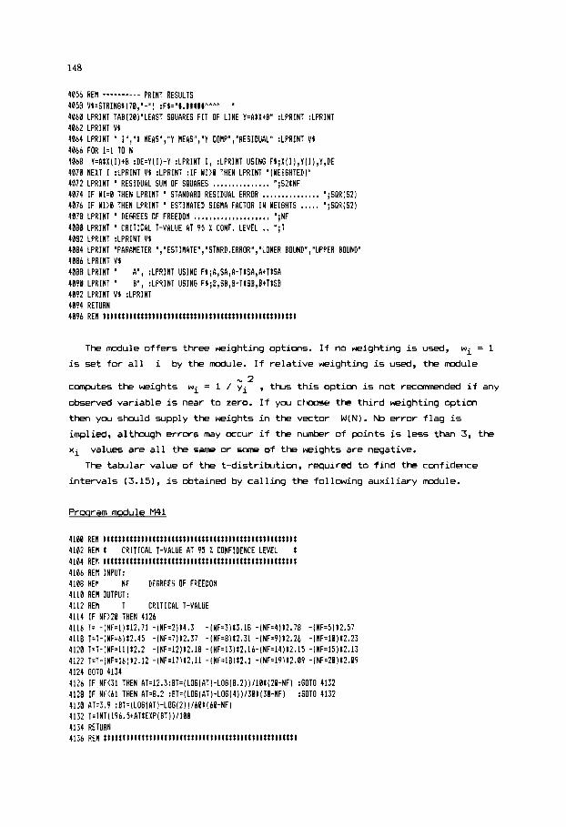
148

4055 HEW ---------- PRINT RESULTS 4058 V$4TRIN6$[7Uq'-') :F$="#.#1111"""* ' 4060 LPRINT TABl2B)"LERST SQUARES FIT OF LINE Y=AtXtB" :LPRINT :LPRINT 4062 LPRINT V $

4066 FOR 1.1 TO N

4870 NEXT I :LPRINT V$ :LPRINT :IF WI>0 THEN LPRINT 4072 LPRlNT . RESIDUAL SUR OF SQUARES ............... ";SZtNF 4074 IF UI=0 THEN LPRlNT . STANDRRD RESIDUAL ERROR ............... ";SOR(S2) 4076 I F WIYd THEN LPRINT . ESTlliATED SIGtlA FACTOR IN WEIGHTS ..... ";SQRISZ) 4078 LPRINT . DEGREES OF FREEDOH .................... ';NF 4080 LPRlNT ' CRITICAL T-VRLUE AT 9 5 1 CONF. LEVEL .. ' ;T 4082 LPRINT :LPRINT V$ 4084 LPRINT 'PARARETER ~l"ESTIRRTEn,,'STNRD,ERROR",'LOWER BOUND" ,"UPPER BOUNDu 4086 LPRINT V1 4888 LPRINT ' 4098 LPRINT a

4892 LPRINT V% :LPRINT 4894 RETURN 4896 RER tttt~ttttttltttttttttltltttttlttttttttttttttttttttt

4064 LPRINT 0 I ~ , H X H E R S ~ ~ ~ Y R E A S ~ , ~ Y c o n P n , v ~ s ~ ~ ~ f i ~ " :LPRINT v$

4868 V=AtXlI)*B :DE=YlI)-Y :LPRINT I, :LPRINT USING F$;XlI),YII),Y,DE

A' , :LPRINT USING F);A,SA,A-TtSA,RtTtSb B", :LPRINT USING FS;B,SB,B-TtSB,BtTtSB

The module offers three weighting options. I f no weighting is used, wi = 1

i5 set for all i by the module. If relative weighting is used, the module

cmpltes the weights

observed variable is near to zero. If you choose the third weighting option

then you should wpply the weights in the vector W(N). No error flag i5

implied, although errors may cccur if the number of points is less than 3, the

xi

- 2 wi = 1 / yi , tb5 this option is not recommended if any

values are all the sane or sane of the weights are negative.

The tabular value of the t-distritutim, required to find the confidence

intervals (3.151, is obtained by calling the following auxiliary module.

Proaram module M41

4100 RE! ttttttttttttttttttttttt~ttt~tttttttlttttt~ttttt~ttt 4102 RE# t t 4104 REM ttttttttttttttlttt&ttttttttttttttltttttttttttt!tttt 4106 RE1 !NPUT: 4188 HEN NF DEGREES OF FREEDOH 4118 RE1 OUTPUT: 4112 HEN T CRITICAL 1-VALUE 4114 IF NF>28 THEN 4126 4116 1- -(NF=I)t12.71 -(NF=2)t4.3 -[NF=3)t3.18 -1NF=4)t2.78 -INF=5)12.57 4118 T=T-INF:b)t2,45 -lNF=7)t2.37 -1NF41t2.31 -INF=9)t2.26 -INFz10)t2.23 4128 T=T-INF=ll)tP.? -INF=12)tZ.18 -1NF=13)t2.lb-INF=14)~2.15 -INF=15)12.!3 4122 T=T-(NF=lb]t2.12 -(NF=17)t2.11 -lNF=18)t2.1 -lNF=19)t2.0? -lNF4)t2.09 4124 GOT0 4134 4126 I F NF(31 THEN AT-12 I 3 : BT:l LO61 AT I -LO6 18.2 ) ll0t I28-NF) :6OTO 4132 4128 IF NF(61 THEN A T 4 . 2 :BT~1L061PT)-L0614))/38tl38-NF) :GOTO 4132 4150 AT4.9 :BT=(LOGI AT )-LO612 ) ) I601 160-NF I 4132 T=INTl196.5tATtEXPlPT) )/I08 4134 RETURN 4136 HE! t t t I It 1 t 1 t It t t t t t t t t It t ttt 11 t tt t t t t t t t t t ttttt ttllt t

CRITICPL T-VALUE AT 95 Z CONFIDENCE LEVEL

149

The only goal of this simple module is to return the t-value found in

statistical tables. Thus, the module could be based m DFIT6 and REFU)

statements instead of the expressions above, but the present form is more

convenient to use if the module is called several times.

Example 3.1 Fitting a straight line by least squares methcd

Table 1.1 lists nicotine and tar concentrations found in different sorts of

cigarettes. ck discussed in Section 1.8.2, me has reason to as- a simple

linear relatimship between the two quantities. First w e assume that the error

variance is constant, and solve the unweighted least squares problem by the

following main program.

180 REW ________________________________________------------------- 1 0 2 REIl EX. 3.1. F I T T I N G A REGRESSION L I N E 1 8 4 REH MERGE H48,tl41 186 HEM ---------- DATA 168 REtl ( N ) 118 DATA 18 112 REM ( X , Y 1 1 1 4 DATA 8.3, 8.32 116 DATA 12.3, 0.46 118 DATA 18.8, 1.10 120 DATA 22.9, 1.34 1 2 2 DATA 2 3 . 1 , 1.26 124 DdTA 24.8, 1.44 1 2 6 DATA 27.3, 1 . 4 2 128 DATA 30.8, 1.96 130 DATA 35.9, 2 . 2 3 132 DATA 4 1 . 6 , 2.28 288 REN ---------- READ DATA 282 READ N 204 DIM X [ N ) , V ( N ) , W I N ) 286 FOR I=I TO N :READ X ( I ) , V ( I ) :NEXT I 288 REM ---------- F I T A STRAIGHT L I N E # I T H NO WEIGHTING 210 WI-0 :GOSUB 4888 212 STOP

It is interesting to compare the following output printed by the module with

the results of Examples 1.8.2 and 1.8.3.

150

LEAST SQUARES FIT OF LINE Y-AtXtB

Y COHP

U.35851EtBB 0.61825EtBB 8.10193EtBl 0.12773EtI l 8.12899Et01 0.13466Et81 8.15542Etfll 0.17242EtBl 8.28955EtBl 0.24542Et01

RESIDUAL

-. 3E515E-81 -, 15025EtBB B. B06E5E-81 0 , b2659E-81 -.2992@E-BI 0.93432E-01 -. 13425EtB8

0.13453Et80 -.25419EtBE

___------_______

8,?3583Et00

RESIDUAL sun OF SQUARES ............... .28~4785 STANDARD RESIDUAL ERROR ............... .158299E DEGREES OF FREEDOfl .................... 8 CRITICAL 1-VALUE AT P5 X CONF. LEVEL .. 2.31

...................................................................... PARMETER ESTIllRTE STNRD.ERROR LOWER BOUND UPPER BOUND

A 8.62933E-81 0.52587E-02 8.50804E-0I 0.75862E-81 B -.16383Et@E 0.13765E+W -.481EBEtBB 0.15413Et00

......................................................................

Thwgh the variances are unknum, considering the small residuals the fit

can be intuitively judged acceptable. This is supported by the lack of trend in

the sequence of the residuals. The slope a is m r e reliable than the

intercept b. In fact the latter estimate heavily depends on the estimation

criterion, as shown in Sections 1.8.2 and 1.8.3. The relations among the

different methods we used to solve this problem will be discussed

3.10.1.

h

h

in Section

Exercises

0 Solve the regression problem with relative weighting (use option WI=1).

Campare the two sequences of residuals.

0 Since tar concentrations are also corrupted by measurement errors, and since

we do not know which variable is more reliable, it is equally meaningful to

fit the inverse model x = Ay + B to the data, thereby regarding the

nicotine concentration a5 independent variable. Show that the two regression

lines differ, t h 5 a ̂ f 1/6 and ^b # -&a . This problem will be further

151

discussed i n Section 3.8.

3.2 MULTIVMIABLE LINAR REGRESSION

Extending the methods of the previws sec t im we f i rst f i t the l inear &el

Y = PIXI + 4 x 2 + * * * + PnxXnx (3.16)

* t o the 5et c (Xi l , xi2, ..., yi) ; i = 1,2,.. .,nm 1 of observations,

where

-w

y i = p1xi1 + @Xi2 + ... + b x x l , n x + €.i . As i n Section 3.1, w e assume that the errors are of zero mean and independent,

with the variances

(3.17)

2 L?{€.i) = Ui = C A W i , (3.18)

where the weighting coefficients wi

function i s

are known. The least squares objective

‘*

Y = , x =

‘1 ,nx . . . Kll x12

K21 x n . . . ‘2,nx

%m, l ‘nm,2 . * ‘nrn , nx

expressions (3.17) and (3.19) are reduced t o

? = x p + c

and

Q(p) = ( ? - X P ) ~ W ( ? - Xp) ,

, € . =

(3.19)

(3.21)

(3.22)

152

respectively, where W is an nmwm diagonal matrix with diagonal entries

W l , - 7

i = 1,2,...,nx , gives the least squares estimates -.-, wnm. Solving the sirmltaneous linear equations 2a(p)/api = 0 ;

The goodness-of-fit is again measured in terms of the residual sum of

squares Q ( $ ) and the variance

(3.24)

of the residuals. ck in the previous section,

constant 2 in the weights, and hence s = sz/wi is an unbiased estimate of

s2 is an estimate of the

2

i

2 -2

i i the error variance u for all i. Having another estimate s of the same

2 -2 variance (e.g. from replicates), the F-test involving the ratio F = s. / s

i i

can be used to check cur assumptions. In practice, however, such independent

estimates s are available in rare circumstances, and the gdness-of-fit is i

* A h

usually assessed by studying the sequence

... - pi,nxxnx , are in use, the basic idea is that in case of a satisfactory fit the

observations should be randanly distibruted around the regression hyperplane

ri = yi - plxil - p2xi2 - ... of residuals. While many diagnosis methods

h

i = 1,2, ..., nm ,

Simple but useful diagnosis twls are the residual plots discussed by wmd

(ref. 6) . If the residuals are of highly nonrandom structure, at least one of the assumptions is questionable. This nonrandumess implies that the el-ts

of the residual sequence rl, r2, ..., rnm are correlated. A measure of this

serial correlation is the D-statistics proposed by Durbin and Watt- (ref. 7),

and cwnpted according to

nm nm T - 1 2

u i D = 1: (ri-ri-1l2 1 ) r .

i=2 i=2

(3.26)

Too large or too small values of (3.26) indicate nonrandumess in the

residual sequence. The critical values of D are tabulated in many textbooks

153

(see, e.g., refs. 5) for nm > 15 . Qssymptotically (i.e., for nm 2 100), the

fit is acceptable at 9% confidence level if 1.7 5 D 5 2.3 , and this interval is larger for smaller samples. Lhfortunately the value of D statistics depends

m the particular order of the observations, which is arbitrary in many cases.

Thus you should be careful with D statistics in multivariable regression.

The most important variability measure of the estimate ^p is its covariance

matrix defined by

This definition already takes into account that in the linear case the least

square estimates are unbiased, t h s

denote the vector of the "true" dependent variables in the sample points, thm

replacing Y by Y' in (3.23) we obtain the true parameters p as estimates.

Using this expression for p and (3.23) for ^p , the definition (3.27) gives

E( ^p ? = p . Let Y' = ( y l , y2, ..., ynmIT

(3.28)

where 6 = Y - Y ' . TIW factor E(GG')

the measurmt errors, and according to (3.18) it is given by

in (3.28) is the covariance matrix of

covCtX> = E{SCT) = . (3.29)

king (3.29) and taking into account that s2 is the estimate of 2, (3.28)

yields the expression

c = 52 (XTkU0-1 (3.30) P

h

to estimate the covariance matrix of p . According to the definition (3.27)

of the covariance matrix, the diagonal entries of C estimate the variances

of individual parameters, and we can also evaluate confidence intervals for

them, similarly to (3.15). The only difference is that now there are nm - nx degrees of freedom.

P

The statistical dependence between the estimates

in term of the correlation coefficients

the estimates

CR lij = rij = c c lij ( c c iiic c ijj11/2 . (3.31)

^pi and Ej is expressed

rij, forming the correlation matrix of

P P P P

If the estimates are strongly correlated then they are far from being

independent and it is better to evaluate their joint confidence region instead

of individual confidence intervals. k show e.g., by Bard (ref. 4), the

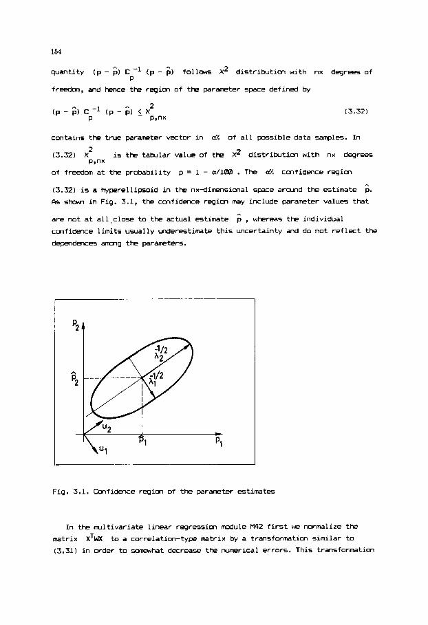
154

quantity (p - 6) C (p - 6 ) follows X2 distribution with nx degrees of

freedom, and hence the region of the parameter space defined by P

(3.32)

contains the true parameter vector in a'/. of all possible data samples. In

(3.32) X is the tabular value of the X2 distribution with nx degrees

of freedom at the probability p = 1 - all021 . The d. confidence region (3.32) is a hyperellipsoid in the nx-dimensional space arcund the estimate

As sham in Fig. 3.1, the confidence region may include parameter values that

are not at all.close to the actual estimate

confidence limits usually underestimate this uncertainty and do not reflect the

dependences amcng the parameters.

2

Plnx

6.

n p , whereas the individual

c

p1

Fig. 3.1. Confidence region of the parameter estimates

In the multivariate linear regression module M42 first we normalize the

matrix

(3.31) in order to sanewhat decrease the numerical errors. This transformation

X'WX to a correlation-type matrix by a transformation similar to

155

is equivalent to a scaling of the parameters, i.e., the unknm variables of

the normal equations. With an ill-cmditioned XTWX , hOwever, the estimates

are strongly influenced by small perturbations in the observations vector ? . This is a frequent problem in parameter estimation, and we use the eigenvalue-

eigenvector decomposition of the normalized

Interpretation of the results of this procedure will be detailed in Section

3.5.

XTWX in order to detect it.

The three weighting options of the module are similar to the ones of the

module We). With no weighting or with relative weighting the array

containing the diagonal entries of the weighting matrix is generated

automatically. This array should be evaluated in the main program only if the

option of user specified weights is used.

W

The parameter FP m g the inpt data is the ridge parameter that will be

exploited in Section 3.5. In normal regression problems FP = 0 should be used.

Proqram module M42

4 2 0 0 REfl t l t t t t t t t t t t t t t t t t t t t t t t t t t t l t l t t t t t l t t l l t t l l l l t t l 4 2 0 2 REH t HULTIVARIABLE LINEAR REGRESSION t 4204 REH 1 WEIGHTED LEAST SOUARES 1 4286 REH t t t t l t t t t t t t t t t t l t t l t t l t t t t t t t t t t t t t t t t t l l l l l l l t t t l 4 2 8 8 REtl INPUT: 4 2 1 1 REH NH NUHBER OF SAHPLE POINTS 4212 REM NX NUHBER OF INDEPENDENT VARIABLES 4 2 1 4 REIl X(Nt!,NXl TABLE OF INDEPENDENT VARIABLES 4 2 1 6 REll Y(NH1 4 2 1 8 HEM WI 4220 REH 4 2 2 2 REfl 4 2 2 4 RER 4226 RER 4228 REfl W[Nt!J 4 2 3 8 REtl RP 4232 REH OUTPUT: 4 2 3 4 REH ER 4236 REH 4 2 3 8 RE1 4 2 4 0 REH P ( N X I 4 2 4 2 REH 4 2 4 4 RER .....

OBSERVATIONS OF DEPENDENT VARIABLE I D E N T I F I E R OF HEIGHTIN6 OPTIONS

@ IDENTICAL WEIGHTS ( W ( I ) = l 1 1 RELATIVE WEIGHTS ( W ( I ) = l / Y ( 1 ) * 2 )

2 USER-SPECIFIED UEIGHTS GIVEN BY FURTHER INPUT AS

VECTOR OF WEIGHTS (ONLY FOR WI.2) RIDGE PARAHETER (ZERO FOR ORDINARY LEAST SQUIRES)

STATUS F L A 6 0 REGRESSION COflPLETED 1 SINGULAR COVARIANCE RATRIX

REGRESSION COEFFICIENTS I N THE EOUATION V = P l t l l t P 2 t X 2 t ... t P n x t X n x

(FURTHER RESULTS ARE PRINTED I N THE t!ODULE] 4 2 4 6 REH AUXILIARY ARRAYS: 4 2 4 8 REIl AINX,NXl ,C(NX,NXI ,U(NX,NX) ,D(NXl 4 2 5 0 REH MODULES CALLED: Rlb,Hl8,H41 4 2 5 2 I F WI.0 THEN FOR K = l TO Nl i :U(I)=l :NEXT K :GOTO 4260 4 2 5 4 I F W I = ? THEN 4 2 6 0 4 2 5 6 FOR K.1 TO Nt! :Y=ABSIYIK)) :IF Y < l E - 1 5 THEN Y=IE-15 4 2 5 8 W ( K J = l / Y I Y :NEXT K

156

426% REH ---------- CONPUTE Y'M AND UX'Y 426; FOR 1=1 TO NX 4264 P [ I ) = 0 :FOR J=l TO I :C(I,J)=0 :NEXT J 4266 NEXT I 4268 FOR K=l TO Nt! 4270 FOR 1.1 TO NX 4272 FOR 3.1 TO I: C(I,J)=C[I,J)tY(K)tX(E,I)tX(K,J) :NEXT J 4274 P(I)=P(I)tW(K)tX(C,I)tY(h') 4276 NEXT I 4278 NEXT C 4280 REM ---------- COVARIANCE RATRlY 4282 TRzlE-30 :FOR 1.1 TO N I : C ( I , @ ) = C ! I , l ) :NEXT I 4264 FOR I=1 TO N I 4286 I F C(!,0)<=TR THEN CIl,fl)=l ELSE C ( I , 0 1 = S Q R ( C ( I , R ) ) 4288 NEXT I 4290 FOR I=l TO NX :FOR J=I TO I 4292 CII,J)=C(I,J)/C(I,0)~C(J,B) 4294 NEXT J :NEXT I 4296 REn ---------- RIDGE STEP 4298 FOR 1=1 TO NX :FOR J=l TO I 4300 C ( I,J)=CI I , JI-RPt(I=J) 4302 NEXT J: NEYT I 4304 RE! ---------- PRINCIPAL COMPONENT ANALYSIS OF THE COVARIANCE I A T R I X 4306 N=NX 4308 FOR 1.1 TO N :FOR J:1 TO I :A(I,J)=C(I,J) :NEXT J :NEXT I 4318 GOSUR l8PB 4312 RE\ ---------- HATRlX INVERSION 4X4 FOR !:I TO N :FOR J = l TO I : R ( I , J ) = C ( I , J ) :NEXT J :NEXT I 4316 GOSUB l6n0 : I F ER=l THEfI 4359 4318 REH ---------- COHPUTE PARAHETER ESTIHATES 4370 FOR 1.1 TO NX 4322 D=O :FOR J=1 TO NX : D = D t R ( I , J ) / C ( J , 0 l t P ( J ) :NEXT J : D ( I ) = D 4324 NEXT I 4326 FOR 1.1 TO NX : P ( I ) = D [ I ) / C ( I , 8 ) :NEXT I 4328 REH ---------- WEIGHTED SUN OF SQUARES AND DURBIN-WATTSON S T A T I S T I C S 4330 FOR K=l TO NH 4332 4334 S 2 = S ? t W ( K ) t D t D 4336 4338 NEXT K 4340 NFZNI-NX :SE=SQR(SP/NF) 4332 I F DN(1E-30 THEN DS:? ELSE DS=DS/DN 4344 REN ---------- STANDARD ERRORS AND CORRELATION HATRIX OF ESTIHATES 4346 FOR 1=1 TO NX 4348 DI I I = S Q R ! S 2 / N F t A ! I , I )/Cil,0)/C( 1,I)) :C(B, I ) = S Q R I A ( I , I ) ) 435I NEXT I 4352 FOR I=1 TO NX :FOR J=l T O NX 4354 C[I,J)~AIl,J)ICIB,I)/CI0,J1 4356 NEYT J:NEWT I 4;58 REN ---------- PRINT RESULTS 4360 V$=STRIN6$170,'-") :F1="l .###l l""A " :FI(=*#.##t *

DE=D :D=Y(K) :FOP 1.1 TO NX : D = D - P ( I ) t X ( k ' , I ) :NE#T I

DN=DN+DtD : I F t31 THEN DS=DSt(D-DE)t (D-DE)

4362 LPRINT TAB(:@);"\ULTIVARIAPLE LINEAR REGRESSION" 4364 LPRINT TbB(?5);'f lETHOD OF LERST SOUARES" 4366 LPRINT :LPRINT :LPRINT 4368 LPRINT 'NUHBER OF INDEPENDENT VARIABLES . . . . . ';NX 4378 LPRINT 'NNUHBER OF SAtiPLE POINTS . . . , . . . ,, I ,, ';Nil 4372 I F RPC0 THEN LPRINT "RIDGE P A M E T E R ..................... ':PIP

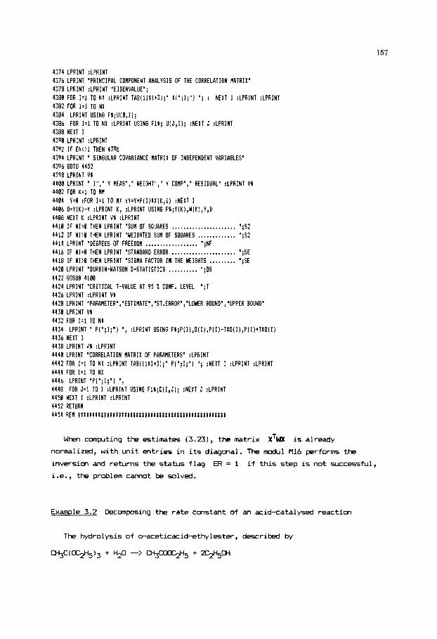
157

4374 LPRINT :LPRINT 4376 LPRINT 'PRINCIPAL COHPONENT ANALYSIS OF THE CORRELATION MATRIX" 4378 LPRINT :LPRINT "El6ENVhLUE'; 4380 FOR 1.1 TO NY :LPRINT TAB(ll11+3);" X(";I;") '; : NEXT I :LPRINT : L P R I N l 4382 FOR I=1 TO NX 4384 LPRINT USING F$;U(B,I): 4386 FOR J = 1 TO W X :LPRINT USING Fl1; UIJ,I); :NEXT J : L P R I N l 4388 NEXT I 4370 LPRINT :LPRINT 4392 I F E R O I THEN 4398 4394 LPRINT ' SINGULAR COVARIANCE MATRIX OF INDEPENDENT VARIABLESB 4396 6010 4452 4398 LPRINT V1 4408 LPRlNT ' In,," V tlEAS',," WEIGHT",' Y COtlP'," RESIDUAL' :LPRINT V I 4402 FOR K = l TO Ntl 4484 Y=0 :FOR 1.1 TO NK : Y = V + P ( I ) t X ( K , I ) :NEXT I

4408 NEXT K :LPRINT V I :LPRINT

4412 IF WI>0 THEN LPRINT 'MEIGHTED SUH OF SQUARES ,.,..,,.,..,. ';S2 4414 LPRlNT 'DEGREES OF FREEDOH .................. ';NF 4418 IF HIM THEN LPRINT 'SIGHA FACTOR I N THE WEIGHTS ,..,.,,., ';SE 4420 LPRINT 'DURBIN-WATSON D-STATISTICS , , , , , . , , , , ';DS 4422 GOSUB 4100 4424 LPRINT "CRITICAL 1-VALUE AT 95 X CONF. LEVEL 4426 LPRINT :LPRINT V1 4428 LPRINT "PARAHETER", "ESTIMATE', 'ST.ERROR", "LOWER BOUND', 'UPPER BOUND' 4438 LPRlNT V1 4432 FOR I=1 TO NX 4434 LPRINT ' PI ' ; I;" 4436 NEXT I 4438 LPRINT V1 :LPRINT 4440 LPRINT "CORRELATION HATRIX OF PARARETERS' :LPRINT 4442 FOR 1.1 TO NX :LPRINT TAB(llll+31;' P( ' ; I ; ' ) '; :NEXT I :LPRINT :LPRINT 4444 FOR 1.1 TO NX 4446 LPRINT " P ( " : I ; " ) y 1

4448 FOR J.1 TO I :LPRINT USING F l $ ; C ( I , J ) ; :NEXT J :LPRINT 4450 NEXT I :LPRINT :LPRINT 4452 RETURN 4454 KEH ltttltlttttlltlttttttlllllllttl~tlltllllllllll~llll

4486 D:Y(K)-Y :LPRINT K , :LPRINT USING FC;Y(K),W(K),Y,D

4410 IF w1.0 THEN LPRINT "sun OF SQUARES ...................... 9 ; s 2

4416 IF 111.0 THEN LPRINT 'STANDARD ERROR ...................... -;SE

';I

" , :LPRINT USING F1;PI I ) ,D( I ] ,PI I ) - T l D ( I ) , P I I ) * T t D ( I )

W h e n computing the estimates (3.231, the matrix XTWX is already

normalized, with unit entries in its diagonal. The d u l Ml6 performs the

inversicn and returns the status flag ER = 1 if this step is not successful,

i.e., the problem cannot be salved.

Example 3.2 Decomposing the rate constant of an acid-catalysed reaction

The hydrolysis of o-aceticacid-ethylester, dexribed by

agC(OcLH5)3 + w --> M3wOcP5 + XTsQ-4

158

is a typical acid-catalysed reaction. As show, by Schwetlick (ref. 81, in the

presence of the weak acid and at Constant ionic strength the rate

constant k of the reaction can be decomposed as Ml$6H4Ui

k = ko + k~[d] + k w C W I , (3.33)

where ko is the rate constant of the uncatalysed reaction, whereas kH and

kW concentration [H'] and that of the undissociated acid concentration [HA],

respectively. In our case HFI is Ml$6H4M. Table 3.1, originally published

in (ref. 91, lists the rate constants observed at different values of

and [W]. Column 3 of the table will be used only in a forthcoming

investigation of Section 3.5.

are catalysis constants that measure the influence of the hydrogen ion

[H+l

Table 3.1

Rate constant of an acid-catalysed reaction

Experimental conditions kx104

[H+]X109 [HFI]X103 [HFI-lX103 11s ml/l ml/l ml/l

4.8 2.42 2.42 1.21 4.8 5.66 5.66 1.20 4.0 16.00 16.00 1.35 4.8 21.21 20.20 1.44 6.5 3.84 2.84 1.54 6.5 10.25 7.56 1.61 6 . 5 18.30 13.50 1.77 10.2 3.10 1.45 2.37 10.2 10.30 4.83 2.47 10.2 30.90 14.50 2.84

_________-__-___-__-l___________l_l

We present a simple main program to estimate the parameters ko, kH and kHFI

by the unweightd least squares method. The program can be used for solving

other linear regression problems if altering the DATA stat-ts appropriately.

The first DRTA line specifies the sample size and the number of independent

variables. The observations are listed in separate DATA lines, where the

first number is the dependent variable. The second number equals 1 and will

result in the cmstant term ko of the rodel (3.33). This is followed by the

values of CH+l and [MI.

159

REH ........................................................... 102 RE\ EX. 3.2. NULTIVARIAFLE LINEAR REGRESSION - ACID CATALYSIS I 0 4 REF NERGE H16,N13,N41,M42 106 REM [NUMBER OF SANPLE POINTS AND NUMBER OF INDEP. VARIABLES) 10@ DATA 10,3 118 RE[ (DEPENDENT VARlAEiE AND INDEPENDENT VARIABLES) 11: DATA 1.21E-4, 1, 4.8E-9, 8.00242 114 DATA 1.20E-4, 1, 4.8E-9, 0.00566 I16 DATA 1.35E-4, I , 4.8E-9, 0.01600 118 DATA 1.44E-4, 1, 4.8E-9, 0.02121 120 DATA 1.54E-4, 1, 6.5E-9, 0.00334 122 DATA 1,61E-4* 1, 6.5E-9, 0.81025 124 DATA 1.77E-4, I , 6,SE-9, 0.01830 126 DATA 2.37E-4, 1, 10.2E-9, 0.00310 128 DATA 2.47E-4, 1, 10.2E-9, 0.01038 130 DATA 2.84E-4, 1, 10.2E-9, 0.03090 209 RE! ---------- READ DATA 202 READ NH,NX 204 DI! X (NF1,NX ) ,Y ( Nli ,UlNM) ,PiNX I 206 DIN AINX,NXl ,C(NX ,NY) ,U(NX,NXl ,DiNX) 208 FOR 1.1 T O NM 210 READ Y ( 1 ) 212 FOR J = l T O NX :HEAD XII,J) :NEWT J 214 NEXT I 216 REH ---------- CALL MODULE (NO WEIGHTING AND NO RIDGE)

220 6OSUB 4200 222 STOP

218 wI.0 :RP=B

The first part of the output contains the principal component analysis of the

correlation matrix discussed later in Section 3.5. In addition to the

residuals, goodness-of-fit, parameter estimates and bcunds, the Durbin-Wattson

D statistics is also printed by the module.

flULTIVARIABLE LINEAR REGRESSION WETHOD OF LEAST SQUARES

NUWBER OF INDEPENDENT VARIABLES . . . . . 3 NUMBER OF SANPLE POINTS 10

PRINCIPAL COMPONENT ANALYSIS OF THE CORRELATION HRTRIX

EIGENVALUE XI 1 1 Y ( 2 I X ( 3 I

8.27101Et01 0.589 0.588 0.554 0.24102Et00 -.374 -.410 0.332 0.48887E-01 -.716 0.698 0.022

1

3 4 5 6 7 R 9 IB

1

0.12100E-03 0.12000E-03 0.13500E-03 0. I4400E-03 0.15400E-03 B.lbl00E-03 0.17700E-03 0.23700E-03 0.24700E-83 0.28408E-03

0.10000Et01 0. I0000E+BI 0.1B0BBEtBI 8.10000Et01 0.108BEE+Bl 0.10B00Et01 B,l8000EtBl 0.100B0Et01 8.18880Et01 8.108iiBEtBl

0.1148BE-03 8.11993E-83 0.1363BE-03 0.14455E-03 8.15513E-83 0.16528E-03 8.17803E-03 0.23685E-03 8.24825E-03 0 I 28087E-83 -----_____.

0.62011E-05 0.70540E-07 -.13030E-05 -.55316E-86 -. 11318E-05 -.42821E-05 -.10294E-05 0.15071E-06 -.1?5BbE-05 B. 31289E-05

sun OF SOUARES ...................... 7.2517e3~-11 DEGREES OF FREEDOM .................. 7 STANDARD ERROR ...................... 3.21863E-Bb DURBIN-WATSON D-STATISTICS .......... 1.158288 CRITICAL T-VALUE A T 95 X CONF. LEVEL 2.37

...................................................................... PARAHETER ESTIMATE ST.ERROR LOWER BOUND UPPER BOUND

P i 1 1 0.34346E-85 8.34861E-05 -.46378E-05 8.11507E-04 PI 2 I 0.224B3Et05 0.45859Et03 0.21316Et05 0.23489Et05 P i 3 1 0.15835E-02 0.11693E-03 0.13064E-02 B.lR686E-02

......................................................................

CORRELATION HATRIX OF PARAKETERS

P i 1 1 P i ? ) P i 3 1

P I 1 1 I. 000 P I 2 -.861 1.080 PI 3 I -.257 -.173 1.080

The standard error is about ZL, which is certainly not larger than the

error in the observed rate coefficients. Therefore, the fit is acceptable in

spite of sme nonrandmess in the sequence of residuals. This conclusion is

supported by the acceptable value of D-statistics, athcugh with only 10 data

points we cannot use this test rigorously.

Though the confidence intervals of the parameters are reasonably small, the

interval for ko includes the value k, = 0, and hmce at the given

significance level we cannot reject the hypothesis ko = 0. Indeed, fitting a

simplified model to the data yields the standard error

s = 3.22x10-6, 50 that the gwdness-of-fit is practically unchanged. Dropping

the constant term is supported by an F-test at any reasonable significance

level. I3 the other hand, a model containing even m r e than three terms might

seem to be natural from a chemist's point of view. We will return to this

question in Section 3.5.1.

k = k,[H+l + k,+CHPl

161

Exercises

Apply (3.23) and (3.30) to the model y = plx + 9 . Compare the resulting expressions with the corresponding expressions of Section 3.1.

Discuss the relation between transforming the matrix XTWX into a

correlation type matrix and scaling of the parameters.

Solve Example 3.2 with the simplified model k = k ~ [ H + l + kwCWIl withart

weighting, then, in turn, apply relative weighting and user specified

weights c

wi = l/ki (also called Poissa, weighting).

o Fit a parabol y = p1 + pzx + ex2 to the data of Examples 1.8.2, 1.8.3

and 3.1 using the program module M42. (See Section 3.9 for a m r e

straightforward solution of this problm.)

3.3 NONINE#? L W T s(xwIES

In this Section we estimate the parameters of the nonlinear vector valued

function

y = f(x,p) (3.34)

c c

The model is fitted to the observations

i = 1 ,..., nm }. Let Ci = ( Lil, ..., €i,ny)T denote the error vector in the i-th observation. We assume that the nymy covariance matrices of the error

vectors are knOwn, at least up to a constant factor. The nm weighting

matrices of dimensions nymy are selected according to

{ (xil, ..., Xi,nx; Yilg * * . , Yi ,ny) 9

-1 COVC Ci 1 = 2 w. ,

1 (3.36)

where 2 is a (possibly unknw) scalar rmltiplier. Note that nondiagonal Wi

matrices are also allowed. The least squares objective function

162

(3.37)

i s i n agreement with the m a x i m l i k e l i h w d principle.

For the sake of s impl ic i ty we introduce the notations

therby reducing the objective function t o the form

The m i n i m of (3.39) can be localized by the methods discussed in Section

2.4. As shown i n many comparative studies (see, e.g., refs. l P k l Z ) , apart f rom

sane special cases ( re f . 13) the most e f f i c i e n t algorithms t o minimize

sum-of-squares objective functions are the various versions of the Gauss-Newton

method. The method i s based on the local l inear approximatim

F(p) H F(p(O)) + J(p(O))Cp - p(O)I (3.40)

of the function F around the i n i t i a l estimate p ( O ) of the parameters. The

(nrnmy)mp Jacobian m a t r i x J of F i s defined by

J(p) = (3.411

Setting (3.40) i n t o (3.39) yields the quadratic approximation

of the objective function, where the argument p(O) of F and J i s dropped

for notational simplicity. TM next estimate p(1) i s then the minirmm point

163

of the quadratic function (3.421, which i s easy t o find. Indeed, regarding = p - p(O) as the u n k n m parameter vector, minimization of (3.42) i s

equivalent t o a l inear regression problem

variables ? - F and the m a t r i x of independent variables J. The solution t o

t h i s problm i s

yields the Gauss-Newton i terat ion

with the vector of dependent

4 = [JTW]-lJTW [? - F]. Repeated application of t h i s idea

where J and F are cmplted a t P ( ~ ) . Similarly t o the quasi Newton

optimization methods, the Gauss-Newton algor i thn of fers quadratic convergence

close to the m i n i m . Further apart, howwer, the step size i s frequently

inflated, part icular ly when [JTWl i s nearly singular. Then p(k+l) might be

a worse approximation t o the m i n i m of (3.39) ttmn i t s e l f . he goal of

the famous Lemberg-Marquardt modification (refs. 14-15) o f the

Gauss-Newton algorithn i s to overcane th i s disadvantage through the i terat ion

p(k)

P ( k + l ) = p(k) + CJTW + ~(~+~)II-~JTW [? - F] , (3.44)

where I i s the npmp unit m a t r i x and the nonnegative scalar x(k+l) i s the

Marquardt parameter. With x suf f ic ient ly large, the additional term

moderates the length of the step and forces i t s direct ion toward the negative

gradient of the objective function. A variety of rules has been proposed fo r

selecting the Marquardt parameter i n subsequent i terat ions (refs. 5,121. I n a

convergent i terat ion most of the methods decrease i t s value, thereby returning

t o the Gauss-Newton procedure.

Chalcqcusly to the l inear case, the goodness-of-fit i s measured i n terms of

the residual sum of squares Q(p) and the residual variance (or sigma square)

5' , defined by (3.24) with the degrees

denominator. Interpretation of estimates is based on the observation that each

i terat ion of the Gauss-Newton algorithn i s equivalent t o solving a l inear

regression problem. Replacing the m a t r i x X i n (3.30) by the Jacobian J(^p),

corresponding t o the l inear approximation of the r e s p s e function F i n a

neighborhood of ^p , the covariance m a t r i x of est imates i s approximated by

h

(nmmy - np) o f freedom i n the

(3.451

Based on the same l inear approximation, the confidence region i s described

by (3.32) a5 i n the l inear case. This i s an approximate relat imship, and may

considerably d i f f e r f rom the exact confidence region given by

164

Q(p) - Q ( ^ p ) 5 X 2 , where

Bard, ref. 51. The exact confidence region has little practical value for

np > 2, since it is very difficult to canpute, whereas the local linear approximation (3.32) will be very useful.

X2 depends on the probability level, (see, e.g.,

The follcwing simple tricks improve the efficiency of the Gauss-Newton-

Marquardt algorithm implemented in the module M45.

(i) The parameters are normalized. In the (k+l)-th iteratim the minimum is

localized in the space of the parameters defined by

Therefore, the initial guess is

entries of the Jacobian matrix are

pj = pj/pj(k).

pj = 1 in every iteration, and the

(3.46)

In spite of the definition of Dj, according to (3 .46) we never divide by

pj. Thus you can choose the initial estimate p, = 0 , but then the j-th parameter remains zero during the iterations.

(ii) The cross product matrix [JT(p)W(p)l is further normalized to a

correlation type matrix before inversion. A t this point we leave

a diagmal entry unchanged if it is less than a threshold selected

relatively to the trace of the matrix. The idea behind this trick is to

allw the additional term x(k+l)I to eliminate the possible near

singularity of the matrix to be inverted.

(iii) The above normalization enables us to use simple rules for selecting the

Marquardt parameter.

Initially x ( 0 ) = 121.01 , whereas in subsequent iterations = O . l x ( k ) if Q(p(k+l)) < Q(P(~)) , and

A(‘+’) = 11211(k) otherwise.

(iv) The sign of the parameters are usually k n m from physical

considerations. Restricting

estimate of the parameters. pj 2 0 we keep the sign of the starting

The termination conditions are

the selected 1-r bound M the relative step size, and IM is the m a x i m

number of iterations.

IIApj ( k ) 11 5 EP or k > IM, where EP is

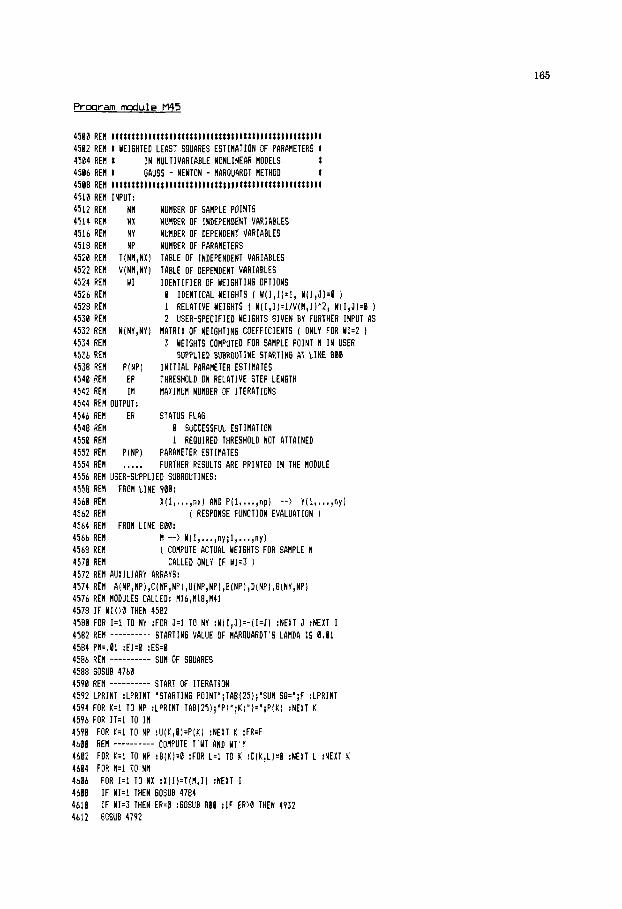
165

Prosram module M45

4 5 0 0 REN t t t t t t t t t t t t t t t t t t t l t t t t t t t t t t ~ t ; t I t t t t t t t t t t t t l t l t 4 5 0 2 REH t WEIGHTED LEAST SQUARES ESTlHl lTION OF PARAMETERS 1 4 5 8 4 RER t I N HULTIVARIABLE NUNLINEAR HODELS t 4 5 6 6 REH t GAUSS - NEWTON - HARQUARDT HETHOD t 4 5 0 8 REM I l t l l t t l t t t t t t t t t t t t t l t t t t t t t t t t F l ~ t t t t ! t ! ~ t t ~ l t t t ~ ~ ; 4 5 1 0 REH INPUT: 4 5 1 2 REN NH NUHBER DF SAHPLE POINTS 4 5 1 4 REH NX NUHBER OF INDEPENDENT VARIABLES 4 5 1 6 REM NY NUHBER OF DEPENDENT VARIABLES 4 5 1 8 REH NP NUHBER OF PAHAHETERS 4 5 2 0 REH T(NH,NX) TABLE OF INDEPENDENT VARIABLES 4 5 2 2 REH V(NH,NY) TABLE OF DEPENDENT VARIABLES 4 5 2 4 REH M I IDENTIFIER OF HEIGHTIN6 OPTIONS 4 5 2 6 REH 0 IDENTICAL HEIGHTS ( W ( l , I ) = l , WlI,JI=U 1 4 5 2 8 REfl I RELATIYE WEIGHTS I H l I , l ~ = l / V ~ f l , l ~ * 2 , Wll,J)=B 1 4 5 5 0 REH 2 USER-SPECIFIED WEIGHTS GIVEN BY FURTHER INPUT AS 4 5 3 2 REH 4534 REH 4536 REH 4538 REN P(NP) I N I T I A L PARAMETER ESTIHATES 4 5 4 0 REH EP THRESHOLD ON RELRTIVE STEP LENGTH 4 5 4 2 REH It4 NAXIMUH NUHBER OF ITERATIONS 4 5 4 4 REH OUTPUT: 4 5 4 6 REM EH STATUS FLAG 4 5 4 8 REH 0 SUCCESSFUL ESTlHATlON 4 5 5 0 REH 1 REQUIRED THRESHOLD NOT ATTAINED 4 5 5 2 REN P I N P ) PARAHETER ESTIHATES 4 5 5 4 REN ,.... FURTHER RESULTS ARE PRINTED I N THE NODULE 4 5 5 6 REfl USER-SUPPLIED SUBROUTINES: 4 5 5 8 REH FROM L I N E 900: 4 5 6 0 REM X i l , ..., n x ) AND F(1, ..., n p ) --> Y l l , ..., n y ) 4 5 6 2 REM 4564 REH FROH L I N E EBB: 4 5 6 6 REM H --> "1, ..., n y ; l , ... ,ny) 4 5 6 8 RER ( COMPUTE ACTUAL WEIGHTS FUR SARPLE t i 4 5 7 0 REH CALLED ONLY I F WI=3 ) 4 5 7 2 REH AUXILIARY ARRAYS: 4 5 7 4 REN A lNP,NP) ,C(NP, NP 1, UINP,NP) ,BINPI, DINP) ,G(NY ,MP ) 4 5 7 6 RER RDDULES CALLED: M l 6 , N l B , R l l 4 5 7 8 I F U I 0 0 THEN 4 5 8 2 4580 FOR 121 TO NY :FOR J.1 TO NY :H(l,J)=-ll=J) :NEXT J :NEXT I 4 5 8 2 REN ---------- STARTING VALUE OF HARQUARDT'S LAHDA IS 0.01 4584 PB=.01 : E l 4 :ES=8 4586 REH ---------- SUM OF SQUARES 4 5 8 8 GOSUP 4768 4 5 9 0 REN ---------- START OF ITERATION 4 5 9 2 LPRINT :LPRINT "STARTING POINT";TAB(25);'SUH SO=";F :LPRINT 4 5 9 4 FOR K = l TO NP :LPRINT TAB(25);"PI';K;')=';PIK) :NEXT t! 4 5 9 6 FUR 11.1 TO I R 4 5 9 8 FOR K = l TO NP :U(K,U)=P[K) :NEXT K :FR=F

4 6 0 2 FOR C=l TO NP : B ( K ) = 0 :FUR L = l TO K :CIK,L)=B :NEXT L :NEXT K 4 6 0 4 FOR fl=1 TO NN 4 6 0 6 4688 4 6 1 0 4 6 1 2 GOSUB 4 7 9 2

Y(NY,NYI HATRIX OF ME16HTING COEFFICIENTS ( ONLY FUR WI.2 ) 3 WEIGHTS COHPUTED FOR SAHPLE POINT H I N USER

SUPPLIED SUBROUTINE STARTING RT LINE 888

( RESPONSE FUNCTION EVALUATION )

4 6 0 0 RE! ---------- COHPUTE T'WT AND N T ' Y

FOR 1.1 TO NX :Xll)=T[fl,l) :NEXT I I F WI=I THEN GOSUB 4784 I F UI.3 THEN ER=U :GOSUB 880 : I F ER)0 THEN 4 9 5 2

166

4614 FOR K = l TO NP 4616 FOR L = l TO K

4628 4622 4624 4626 NEXT L 4628 A=0 4638 FOR 1.1 TO NY:F@R J = 1 TO NY 4 6 2 4634 NEXT J :NEXT I :P(K)=RlK)+A 4636 NEXT C 4638 NEXT ti

4642 TR.0 :FOR 1.1 TO NP : C l l , O ) = C ( I q l ) :TR=TR+C!I,I) :NEXT I 4644 TR=TR/NP/ IB08 4646 FOR 1=1 TO NP 4b48 4650 NEXT I 4652 FOR 1=1 TO NP :FOR J = l TO I 3654 4656 NEXT J :NEXT I

4668 FOR 1.1 TO NP 4662 FOR J=I TO 1-1 : I l ( l , J ! = C i l , J ] :NEXT J

4666 NEXT I 4668 REIl ---------- I A T R l X INVERSION 4670 ER.8 :N=NP :GOSUB 1600 : I F EP=I THEN 4718 4672 REH ---------- CORPUTE STEP 4674 FOR I:1 TD tip 4676

4bie ~ = 0 FOR I=1 TO NY:FOR J = l TO NY

NEXT J :NEXT I :ClK,L!=ClK,L!tA A=AtM( I , J It61 I , L ) $61 J , K ) t P ( L ) l P l K )

8=6tW! I , J It6l J ,K) t lVlH, I !-Y l I ) ! W ! K !

NORMALIZE 4648 REM --____----

IF C/I ,U)(=TR THEN C(l,B!=l ELSE C!I,0)=SQR(ClI,P!!

U l I , J )=C( I , J 1 :C! I , J!=Cl I , J1 / C I I ,0) / C ( J ,B)

4658 REN ---------- I IAROUARDT 'S COt4PRONlSE

4504 AI I , I I = C ( r , I i t ~ n

D 4 :FOR J = 1 TO NP : D = D t A I ~ , J ) / C I J , @ ) t R ! J ! :NEXT J :DII)=DICiI,A! 4678 NEH I 4680 4682 SL-0 :ll=l 4684 FOR 1.1 TO NP 4686 IF r I tD! I ) ( : - .?5 THEN XI=-.95/D(I) 4688 S L = S L t D ( I ) t D ( I ) 4690 NEXT I : S L = S O R I S L l t X I 46V RER ---------- NEW ESTIIIATES 4694 FOR 1.1 TO NP : P l l ~ = U l l , B ~ t ( l t X I t D ~ I ~ ) :NEXT I 4696 GOSUB 4760 4698 RER ---------- PRINT ITERATION STEP 4708 F$=n# . l " *A" :LPRINT 4782 LFRINT "IT=';IT;TRRilB);"P#="; :LPRINT USING F$;PH; 4704 LPRINT T I l B ( 2 5 ) :"SUM SQ=";F;TAP( 501 ; "SL=";SL :LPRINT 4786 I F F>=FR THEN 4710 4788 FOR K=l TO NP :LPRINT TRBIZS);'PI';;K;")=';;PiK) :NEXT K 4718 PEN ---------- END OF PRINT 4 7 2 IF SL!=EP THEN E l 4 :60TO 4726 4714 REH -______--- RAROUARDT'S PARAIIETER 4716 IF F V R THEN 4720 4718 PH=10tPH :GOTO 4658 4720 P t k P t i i l 0 :IF Ptl(.B0!001 THEN Pfl=.000001 4722 NEXT I T 4724 EI=I 4726 IF F F R THEN 4738 4728 F=FR :FOR 1=1 TO NP :PlI)=UlI,B) :NEXT I

REH ---------- CHECK S16N AH0 REDUCE STEP IF NEEUEU

167

4730 REM ---------- STANDARD ERROR AND CORRELATION MATRIX OF PARAMETERS 4732 NF:NtltNY-NP :SE=SQRlF/NF) 4734 FOR 1.1 TO NP :FOR J = l TO I :Al1,J)=ClI,J) :NEXT J:NEXT I 4736 GDSUB I600 :IF E R = I THEN ES.1 :GOTO 4752 4738 FOR I = I TO NP 4740 B ( I ) = S Q R ( F / N F t A l I , I )/ClI,0)/C( I ,8)) 4742 C ( B 3 I )=SORIA( I I I ) ) 4744 NEXT I 4746 FOR I=l TO NP :FOR J = 1 TO NP 4748 C l I , J)=A( I , J 1 /Cl8, I ) / C l 0 , J ) 4758 NEXT J:NEXT I 4752 REH ---------- PRINCIPAL COHPONENT ANALYSIS 4754 FOR I = I TO NP :FOR J = I TO I :A(I,J)=U(I,J) :NEXT J :NEXT 1 4756 N=NP :GOSUB l88e 4758 GOT0 4818 4760 RER ---------- COMPUTE SSQ 4762 F=0 4764 FOR 1.1 TO NH 4766 FOR I=1 TO NX : X l I ) = T l H 4 1 ) :NEXT I 4768 I F W I = l THEN GOSUB 4784 4778 IF W1.3 THEN GOSUB 800 4772 GOSUB 908 4774 FOR 1-1 TO NV :FOR J=1 TO NY 4776 F ~ F t # l I , J ~ t ~ V l ~ , l ~ - Y l ~ ~ ~ t l V l M , J ~ - Y I J ~ ~ 4778 NEXT J :NEXT 1 4780 NEXT M 4782 RETURN 4784 REH ---------- RELATIVE WEIGHTS 4786 FOR I=1 TO NY :V=ABS(V( i l , I ) ) : I F Y(1E-15 THEN Y=lE-15 4788 W ( I , I ) = l / V / Y :NEXT I 4798 RETURN 4792 REIl ---------- COHPUTE JACOB1 MATRIX GINY,NP) AND RESPONSE Y(NY) 4794 FOR J=I TO NP 4796 D E ~ . 8 0 l t A B S l P l J ) ) t l E - l 0 : P I J ) = P l J ) + D E :GOSUB 900 4798 FOR I=1 TO NY : 6 ( 1 , J I = V l I ) / D E :NEXT I 4800 P I J ) = P I J ) -DE :D I J ):DE 4882 NEXT J 4884 GOSUB 988 4886 FOR 1.1 TO NY :FOR J=I TO NP :6(1,J)=GII,J)-YlI)/DIJ) :NEXT 3: NEXT I 4888 RETURN 4810 REM --------- PRINT RESULTS 4812 LPRINT :LPRINT 4814 LPRlNT TAB(15);"WEIGHTED LEAST SQUARES PARAMETER ESTIMATION' 4816 LPRINT T A B ( 2 1 ) ; ' I N f lULTIVARlABLE NONLINEAR MODELS' 4818 LPRINT TRB(21);'6AUSS - NEWTON - MAROUARDT HETHOD" 4821 LPRINT :LPRINT :LPRINT 4822 LPRINT 'NUMBER OF INDEPENDENT VARIABLES . . . . , ";NX 4824 LPRINT "NUMBER OF DEPENDENT VARIABLES , . . . . . . ';NY 4826 LPRINT 'NUMPER OF PARAIIETERS ,. . . ,. ..,...., I I ';NP 4828 LPRINT "NUMBER OF SAMPLE POINTS ,. ,. . . . . . . . . . ':NM 4830 LPRINT "OPTION OF WEIGHTING .. ... . . . . . . . . . . . . ';HI; 4832 IF UI=0 THEN LPRINT " I I D E N T I C A L WEIGHTS)' 4834 I F W I = l THEN LPRINT ' [RELATIVE WEIGHTS)" 4836 IF MI=2 THEN LPRlNT '[USER DEFINED WEIGHTS, INDEPENDENT ON THE SAMPLE" 4838 IF W1.3 THEN LPRINT *(USER DEFINED WEIGHTS, DEPENDENT ON THE SAMPLE' 4848 FS='#.#tll#"A*A * :FI$="#,### ':LPRIMT :LPRINT 4842 LPRlNT *PRINCIPAL COMPONENT ANALYSIS OF NORHED CROSS PRODUCT HATRIX"

168

4 8 4 4 LFRINT : L P R I N T "EIGEN!'ALUE"; 4 8 1 b FOR I=! TO UP :LPRlWT T f i E ( l l t l + ; ) ; " P ( " : I : " j " ; : NEXT I :LPRINT :LPRINT 4 8 4 3 F1R I = 1 TC NP 4 8 5 0 LF'RINT USING FIiUIB,:), 4 8 E FOR J = 1 T O I P :LPPINT USING F l ' l ; UiJ,I); :NEXT J :LPRINT 4851 NEXT I 4856 LPRINT :LPRINT 4 8 5 8 Yt=STRING$170," - " ) :V! i=STRIN6)(55," - " ) 4 3 6 0 IF E I = l THEN LPRINT " REQUIRED THRESHOLD NOT RTTAINED" :LPRI#T :;PRINT 4 8 6 2 I F ES.1 TBEN LPRINT " SIISULRR CRCSS PRODUCT H f i T R I i " :LPRINT :LPRINT 4 8 5 4 FOR 151 TO N'/ 4 8 6 5 LF'RINT :IF NY)! THEN L P l I N T "RESPONSE FUNCTIOI4";I 4 8 6 8 LFP!NT ill$ : L P R I I T "SAMPLE #a' ," Y HEAS"!" Y C@)rP', ' ' R E S I D i l k L " :LFHINT V1$ 4 8 7 0 FUR H=l TO NM 487: FOR J=1 TO N X :X(J;=7(MtJ) :NEXT 1

4 8 7 6 LPRINT !I, :LPR!NT USI#G F I ; ' ~ ~ M , I ) , Y ~ I ! , V ~ ~ , I ! - Y I . ~ ~ 4 8 7 4 SDSUB 9 n a

4 8 7 8 N E X T n :LPRIWT vis 4 e 3 B NEXT I :LPRI#T :LPPiNT 488: IF II.0 THEN LFRINT "SU! OF SQURRES ...................... ";F 4 8 3 4 I F WI%l THEN LPRINT WEIGHTED SUM OF SQUARES ............. ";F 4 8 3 6 LPPINT "DEGSEES OF FREEDOM .................. ";NF 4 a a 8 IF WI=O THEN LPRINT "STBNDABD EWIR ...................... ";SE 4 8 9 0 I F $1 : a THEN LPRINT "SISMfi FACTOk I N THE WEIGHTS ..... 4 8 9 2 GOSUB 4 1 0 0 4 3 9 4 LPRINT " C H I T I C A L 1-VALUE RT 95 7, CONF. LEVEL 4 8 9 6 LFRIHT :LPRINT Vd

4 W @ I F ES.0 THEN LPRINT "ST. ERROR","LOUER BOUND","UPFEP @OUND*: 4 9 0 2 LF'RINT :LPRINT V $ 4904 FOR 1=1 TO NP 4 9 0 5 LPRINT " P [ ' i I I ; " ) *, :LPRINT !SING F$;P(l), 4 9 0 8 PR=ARS(Rl I )tPi 1 ) ) 4 9 1 3 4 9 2 LPRINT 4 9 1 4 NEXT I 4 9 1 6 L P R I I T Vf :LPRIIT 4919 IF ES=! THEN ER.1 :GUT0 4 9 3 7 4 9 2 0 LPRINT "CORRELATION MATRIX OF PPIRRHETERSn :LPRINT 4 9 2 2 FOR 1.1 T3 NP :LPRINT T A B ( l l t I t 3 ) ; " P ( " ; I ; " ) "; :NEXT I :LFRIWT :LFRINT 4 9 2 4 FOR 111 TO NP 49% LPPINT 'P!" ; I ; " ) ", 4928 FOR J = 1 TO I :LPRINT USING FI$:C(IIJ): :NE?T J :LPRINT 4 9 3 0 NEXT I :LPRINT :LPRI#T 4972 RETURN 49:4 REH t t t t t ~ t t t t t l l t t t t l ~ ! ( t t t t t t l t t t t t t t t t t t t t t t t t ~ t l ~ t l

";T

4 3 9 8 LPRINT ~PPARAIIETEP", W I ~ ~ R T E " ,

I F ES.0 THEN LFRINT USING FI;PF,PII)-TLPB,P(I)tTtPB;

The ro le of the i n p l t data NVI, NX, NY and N) i s obvious frm the text and

the remark lines, but the array T("1,NX) of independent variables deserves - explanation. Each l i n e of the array should contain a l l information that

enables us to canplte the value of the dependent variables for a sample p i n t

a t the current values of the parameters. Therefore, the module transfers the

appropriate row of T(NVI,NX) i n t o the vector X(NX) fo r further use i n the

user supplied subroutine. This subroutine start ing a t l i n e 920 cmpl tes the

independent variables Y ( N Y ) a t the current parameters P(W) and independent

169

variables X ( N X ) . If the model consists only of one response function, then

NY = 1 and only Y ( 1 ) is evaluated in the user subroutine. The observed

values of the dependent variables are stored in the array V(”l,NY). If there

is only one response function, this array consists of one column.

There are four weighting options. No weighting (WI = 0) and relative

weighting (WI = 1) are easy to use, because the weights are generated

automatically. Y o u should remember, hOwever, that relative weighting is not

recormended if any observed value is near to zero. With the option WI = 2

y w should provide an N Y W Y matrix of weights in the array W(NY,NY). The

same weighting matrix will be then used in all sample points.

Y o u may also wish to use different weighting matrices for different

observations. For this pIrpose the weighting option WI = 3 is provided. To

use this option you rmst supply a second subroutine starting at line 600 , where you have access to the index M of the current sample point. The task of

the second routine is to compute the N Y W Y weighting matrix for the current

sample point and to place it into the array W.

Selecting the initial estimates of the parameters P(W) you should keep in

mind that their signs remain unchanged during the iterations. For a first try

it is reaMnable to set a low limit on the number of iterations, say IM = 5 , and to use a moderate value, say 0.01 or 0.001 , for EP.

The subroutine bet- lines 4792 - 4808 provides divided difference

approximation of the appropriate segment of the Jacobian matrix, stored in the

array G(NY,I\P). In saw applications the efficiency of the minimization can be

considerably increased replacing this gmeral purpose routine by analytical

derivatives for the particular model. In that case, hawever, Y ( N Y ) should be

alsn updated here.

Example 3.3 Fitting a nonlinear rate expression

Rational functions are frequently encountered as rate expressions of

catalytic reactions. In addition, the function

(3.48)

is a popular test problem for comparing parameter estimation procedures

(refs. 10,12). In this case we have only m e response function, three

independent variables and three parameters. Line 110 of the following main program

smifies these values, together with the number NM = 15 of observations.

The 15 MTFI lines starting at line 114 correspond to the 15 observation

pints. The values of the dependent variable and of the independent variables

can be easily reconstructed from the listing. Since NY = 1 , the subroutine starting at line 90 compltes the single value Y ( 1 ) . Selecting the unweighted

option WI = 0 we do not need the second user subroutine. The starting

estimate of the parameters i5 given in line 220.

170

100 REfl ___-_______-____________________________......-~~----------

102 HEM Ef. 3,3, NONLINEAR LS9 PARAHETER ESTlH4TION - RRHD EXARPLE 104 REN MERGE fll6,Nlfl,N41,N45

IE8 REH I N M , NY, NX, NP) l!O DATA 15, 1, 3, 3 11; REN ! Y , XI, X:, X3 1 114 DATA 0.14, 1, 15, 1 I16 DATA 0.18, 2 , 14, 2 118 DATA 0 . 2 , 3, 13, 3 l?tl DkTA fl.X, 4 : 12, 4 !Z DATA 0 , 2 9 , 5 , 11, 5 124 DATA 0 . 2 , 6 , 18, b !:A DATA 3.15, 7, 9, 7 128 DATA 0 . 3 9 , R, 8, 8 1:0 DATA E . 3 , 9 , 7, ?

1:: DATA 0.58, 10, 6 , 6 134 DATA 0 , 7 3 , 11, 5, 5 1:b DATA 0 . 9 6 , I ? , 4 , 4 I 8 DATA 1.34, 13, 3, 3 140 DATA 2 - 1 8 , 1 4 , 2 , 2 142 DATA 4 . 3 , 15, 1, 1 288 HEM ---------- READ DATA 282 READ NN,NY,NI,NP 2R4 DIN TINII,NX i ,ViNn,NY ,PINPI, X INX , Y “I! , W(NY,NY! X b DIR A! BPI NP , C(NP,NP I , U [ NP, NP! , R (NP i , D (NP! ,GI NY ,NF) 208 FOR I:l TO NM 210 FOR J.1 TO NY :READ V ( l , d ! :NEXT J 212 FOR d=l T@ NT :READ TII,J! :NEXT J ;I4 NEXT I 216 REIl ---------- CALL NONLINERR LSQ EST!HATIOH MODULE 218 WI.0 :EP=.BB0I :Itl=20 220 Pili=l :P12!=1 :P i ; i= l 222 GOSUB 4580 224 STOP 90R BEH ---------- FUNCTION EVALUATION 902 Y ( 1 )=PI! )+XI I)/( P ( 2 ) tX (2jtP( 3) tX ( 3 ) ) 904 RETURN

106 REF ---------- DATA

kcord ing t o the following cutplt, the module needed s i x i terat ions t o f ind

the m i n i m of the objective f u n c t i m . The value of the Marquardt parameter

PM, i.e., A ( k ) i s gradually decrased. I n i terat ions

attempts wi th d i f ferent Marquardt parameters are necessary t o improve the

objective funct im. I n less cooperative estimation problems the module

frequently needs t o increase the Marquardt parameter. The current value of the

sum of squares, i.e., the objective function and the re la t ive step length SL

are also printed i n every i terat ion.

5 and 6 several

I f a less conservative terminatim cr i ter ion, say EP = 0.ml were used,

the prazedure would be stopped af ter the 5 t h i t e ra t i on as seen f rom the value

of SL.

171

S T A i t T I N G POINT

IT= 1 PII=B. IE-@l

IT= 2 PN=@.lE-I2

I T = 3 Pti4.IE-13

I T = 4 Pti=@.IE-64

IT. 5 PH=E.lE-05

I T = 5 Pk0.lE-04

I T = 6 PM=B.lE-85

I T = 5 PM:O,lE-04

I T = 6 PM=l.IE-13

IT. 6 PH4.lE-02

IT= 6 Ptl=B.IE-01

S L l l SO: 41,5817

P i 1 ) = 1 Pi 2 ) = 1 P i : ) = 1

SUM SO= 1.345128

P i 1 I = ,1051949 P ( 2 1: 1.42418 P i != 1.4323;

SUN SO: 3.852356E-02

P i 1 ) = 9.08139E-12 P i 2 ) = 1.47196 F'i : != 1.90143

P i 1 != 8.343399E-02 P i 2 I = 1,14498:: P i 3 ) = 2.338202

SUM 50: 8.214884E-13

P ( 1 != 8.244011E-02 P! 2 I= 1.133951 P i 3 I= 2.342925

SUN 50: 8,214894E-03

SUM SO= 8.?14876E-03

P! 1 ) = 8.241451E-02 P ( 2 ) = 1.133249 P i i; ) = 2.343488

SUM SO: 8.214985E-03

SUM SO. 8.214876E-03

Slifl SO= 8.214886E-B3

SUfl SO. 9.214867E-13

SL= 1.07967:;

SL= ,3596549

SL= , 326665

SL= 1.660105E-02

SL: 7.513525E-84

SL. 7.476811E-14

SL= 2.55171E-84

SL. 2 I 539624E-84

SL= 2.426527E-04

SL= 1.711297E-04

SL= 6.648381E-85

172

WEIGHTEU LEAST SQIJAFES PARAMETER ESTIMAT!ON I N MULT!VARIABLE NONLINEM HODELS GAUSS - MENTON - HARQUARDT METHOD

NUMBER OF !\DEPENDENT V A ~ l P B i E S ..,.. 3 NUHBER OF DEPENDENT ?'BRIfiRLES , , , I . . . 1 NUNBER OF P4PMETEPS . , . . , . . . . . . , . . . . 3

O P T I O N OF WEIGHTING ,.,,,,,......,... 0 (IDENTICAL WEIGHTS) NUNPER OF Sf i l lP~E PGINTS ............. : 5

PRlNClPAL CGNPOYERT ANALYSIS OF NORHED CROSS PRODUCT HATR! Y

EIGEMVALUE P I I ! P ( 2 i P i 1

0.14589Et02 -.048 0.437 0 . 8 W 0,79533E-01 8.973 - ,XS 0.707 0.6592:E-02 0,383 0.839 - . B E

.___________________----------------..-----.-...---.---

SAtlPLE No Y MEAS Y C O W RESIDUAL

I 2

4 5 6 7 8 9 10 I!

13 14 15

>

( 7 A.

1, 14BEEE+00 0. 18000E+8@ 0. ?:O00Et00 0.?5000E+00 0 , ?9000E+00 0.12000Et00 E . 350@0E+@0 0 . 3 0 0 0 E t 1 0 0.37000Et00 a . Z80@@E+@@ 0,7:000E+O0

0.13400E+01

0.4Z900Et01

B . P ~ R ~ C E + E ~

@.71@0@EtOl

0.13411E+B@ @.1797?E+00 0.?7926E+00 0,?5653E+PB 0 I 78917EtE0 1.31Eb9E+00

0,3!004E+00

0.56179E+10

B , 94529Et10 0.1!2iiBE+Bl A. 20?58E+Q1 0 ,43968EtB I

0.34553E+00

%.45!27E+0@

a , 7 i w ~ t @ a

0.588BSE-02 0,2761 5E-03 -. Zb?71E-Y13 -. 6S301E-0: 0.83?74E-03 0.130b7E-07 0.44672E-82 0.19964E-81

0.18?1?E-01 0.14812E-01 E.14710E-01 0 . 1 1 ~ 0 8 E - O l 0.42033E-02 -.68097E-0?

-.mi 5 ~ 4 1

SUfl OF SOUARES . . . , . . . . . . . . , . . . . . . . . . DEGREES OF FREEDOM , , . I ,,, ,. ,. . . . . . ,. STAliDi lRD ERROR ,., . . . . . . ,.. . . . . . . . . . . C R I T I C R L T-VALUE Pl 95 7, COIF. LEVEL

8.214867E-03 12 2.616433E-02 2 - 1 8

PI 1 ) 0.62410E-01 0.1Zt9E-01 0.55446E-81 @.1@9;7E+00

P i Z ) 0.?:.435E+@l 0.29666Et00 0.16968Et01 '2,?990?E+01 P i 2 0.11::2E+01 0.:0815E+00 0.46145€+08 0.18050Et01

CORRELRT13N MATRIX DF PRRANETERS

173

Most part of the output i s similar t o the artput of the l inear regression

module. The eigenvalues and eigenvectors refer t o the m a t r i x

w i l l discuss i n Section 3.5 how to use t h i s information.

[JT(fi)WI(fi)]. We

Exercises

0 Show that increasing the Marquardt parameter moves the correct im vector

tward the direction of the negative gradient of the objective function

while the length of the correction vector decreases.

Ap

0 The Hessian m a t r i x of the quadratic approximation (3.42) of the objective

function equals

objective function (3.39). Show that the Gauss-Newton method can be

interpreted as a quas i -Wtm method of minimization that neglects a certain

term i n the Hessian. Can you j u s t i f y t h i s approximation i f the residuals are

5M1 l ?

fi = 2JTW . Compare t h i s with the t rue Hessian m a t r i x of the

0 Rerun Example 3.3 with d i f ferent start ing estimates. Does the number of

i t e r a t i m s depend heavily M the start ing estimate i n t h i s problem?

3.4 LINARIZATICN, WEIGHTING AND REPNWETERIZATIaU

Though module M45 i s an e f f i c i en t tml, f i t t i n g a nonlinear model t o data

usually requires considerable computational ef for ts, and w i t h w t a good i n i t i a l

guess even the convergence i s questionable. Therefore, a transformation

replacing the problem with a l inear regression one i s of great practical value.

A well known example i s the Arrhmius dependence

k = kxpC-E/(RT)] (3.49)

of the chemical k inet ics rate coeff ic ient k on the temperature T, where

R = 8.3144 J / ( m l K) i s the universal gas constant, and the preexponential

factor A and the activation energy E are the u n k n m parameters. These

parameters are a l m t invariably determined by f i t t i n g the l i n e

y = ax + b ; with y = log(k1 and x = - l / T , (3.50)

where E/R = a and log(A) = b. A number of simple functions are l inearizable

by suitable transformations (see e.g., re f . 5 ) with part icular ly many

applications i n the k inet ics of enzyme reactions ( re f . 16) and cata ly t ic

processes ( re f . 17) .

F i t t i ng the expressions (3.49) and (3.50) t o experimental data we obtain,

174

hMrJever, somewhat different estimates, since the transformation distorts the

error distribution, and the original assumptions do not m r e apply.

In this section we show how the deviations stming f r m linearization can

be compensated by selecting suitable weighting coefficients. The observartions

are of the form

5

Yi = Yi + Li , (3.51)

2 where yi = f(xi,p), and D2{ Li 1 = u . Instead of fitting y = f(x,p) to

i

5

the data yi we rather fit the transformed model y ' = g[ f(x,p) 3 to the

traneformed data yi' = g[ ;i 3 , where g[ I is the linearizing

transformation, and

5

.., = g [ yi 1 + Li' .

To find the variance of Li' note that by (3.51)

(3.52)

5 5

€1' = g [ yi 1 - gc yi - €1 1 , (3.53)

- * -" where

g ' = dg/dy . Therefore, from (3.53) Ci' S g ' [ yj ILi and

g[ yi - ci 3 5 g[ yi 3 - g'[ yi from the linear approximation and

5

Thus, fitting the transformed model to the data the original

assumptions are better retained through the use of the weighting coefficients

wi = 2/( g'[ ;i lai )' , where

gC ;i 3

2 is an arbitrary positive constant.

Example 3.4 Estimation of Arrhenius parameters by weighted linear regression

Table 3.2 lists the rate coefficient of the reaction

ag1 + cp5ma ---> cH30c$i5 + NaI

at 6 different temperatures (ref. 18). First we assume that k 1s

observed with constant error variance. Equation (3.49) is fitted to the data

using nonlinear least squares with weighting coefficients wi = 1. In

addition to the nonlinear fit we estimate the parameters from the logarithmic

model (3.m).

175

Table 3.2 Observed temperature dependence of rate coefficient

T, K 273.15 279.15 285.15 291.15 297.15 m . 1 5 kx105, l/(ml 5 ) 5.6 11.8 24.5 48.8 102 m

Fitting (3.50) w e first use the weights

frm (3.54) . This is done by the m u l e M40 with options WI = 0 and

W I = 2, respectively. Table 3.3 lists the estimates and the 9SL confidence

intervals that are not symmetric, due to the exponential back transformation.

wi = 1 , and then wi = zi2 following

Table 3.3 Estimates and 95% confidence intervals of the Arrhenius parameters

Nonlinear estimation Linear estimation

0x10-12, l/(ml 5 ) 3.42 0.317 0.325 3.10 (-2.2, 9.1) (-0.12, 0.75) (0.09, 1.2) (0.61, 16)

EXI~-~, mi 8.83 8.25 8.25 8.81 (8.4, 9.2) (7.9, 8.6) (7.9, 8.6) (8.4, 9.2)

As seen from the first and last columns of the table, the appropriate weighting

considerably reduces the deviations between the results of linear and nonlinear

estimations.

The table also shows that the nonlinear fit gives a very large confidence

interval for the parameter A, an inherent problem in fitting the Arrhenius

expression (3.49) directly. While the extremely large Confidence interval is an

overestimation stming from the local linear approximation of the &el, it

still reveals a real problem. As discussed in the previous section, the

Gauss-Newton method involves a sequence of quadratic approximations of the

objective function. Each of such approximations is a long valley along the

coordinate axis corresponding to A, and its minimum is rather difficult to

localize with reasonable accuracy. This problem, reconsidered in the next

section, increases the significance of the simple linear estimation through

logarithnic transformation.

The "observed" rate constants are, in fact, derived from other measurable

quantities, and according to chemists the assumption of constant relative

variances (i.e., criz is proportional to ki') is usually closer to the reality

than that of constant variances. Assuming such error structure one chooses the

weighting coefficients wi = zi-'

" 3

when fitting (3.49) directly, and hence unit

176

weights wi = 1

considerations and the corresponding results show, in the second and third

colunns of Table 3.3 justify the use of unweighted linear regression for

estimating Arrhenius parameters.

in the linear regression involving (3.50). These

lhfortunately, many transformations purported to linearize the model also

interchange the role of dependent and independent variables. Important examples

are the various linearization transformations of the simple steady-state

Michaelis-Mentm d e l

(3.55)

of the enzyme reaction studied in Section 2.5.1, where [ S ] denotes the

concentration of the substrate and r is the rate of the reactim. To estimate

the Michaelis-Mentm parameters V and K from the data C (CSil, ri);

i = 1,2, ..., nm >, me can fit, for example, the following linear functions

(ref. 19):

*

(Hanes),

(Scatc hard )

(Lineweaver-Eurk)

(3.57)

(3.58)

(3.59)

These classical methods are still poplar. Since the error in the observed

reaction rate ri

concentration CSil, assumption (i) of the least squares method is

approximately satisfied w h e n fitting (3.55) directly. This assumption is,

however, clearly violated in models (3.56 - 3.581, where the error corrupted r appears also on the right hand side. Therefore, the use of mst linearized

models should be restricted to determining a good initial guess for the

nonlinear parameter estimation (ref. 20).

* is usually much larger than the error in the substrate

Linearization by transformation and rearrangemmt of the variables is not I

the mly way to reduce computational efforts in nonlinear estimation. A faster

convergence can be expxted if the nonlinear character of the model is

decreased by manipulating the parameters. Bates and Watts (ref. 21) proposed a

measure of nonlinearity and found that the major part of nonlinearity was due

to the particular parameterization in many models. In such caws nonlmear

parameter transformations may considerably improve the efficiency of the search

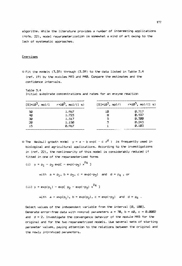
177

algorithm. While the literature provides a number of interesting applications

(refs. Z ) , model reparameterization is somewhat a kind of art owing to the

lack of systematic approaches.

Exercises

0 Fit the models (3.55) through (3.59) to the data listed in Table 3.4

(ref. 19) by the modules M45 and M40. Compare the estimates and the

confidence intervals.

Table 3.4 Initial substrate concentrations and rates for an enzyme reaction

~ ~ 1 x 1 6 , moi/i r~105, mi/(i s)

32 1.967 40 1.723 3m 1.517 m 1.1m 15 0.967

10 8 5 3 1

0.717 0.537 O . m 0.243 0.103

0 The kibull growth model y = a - b exp( - c xd ) is frequently used in

biological and agricultural appl icaticns. According to the investigations

in (ref. 2 2 ) , the nonlinearity of this model is considerably reduced if

fitted in one of the reparameterized forms

with a = pl, b = 6, c = exp(-p3) and d = p4 , or

Selezt values of the independent variable f r m the interval CO, lml.

Generate error-free data with nominal parameters a = 70, b = 60, c = 0.awa)2

and d = 2. Investigate the convergence behavior of the module M45 for the

original and for the two reparametrized models. Use several sets o f starting

parameter values, paying attention to the relations between the original and

the newly introduced parameters.

1 I0

3.5 ILL-CONDITIOND ESTIMFITION PROBLEMS

To obtain the estimate (3.23) in a multivariate linear regression problem w e

h

solve a set of linear equations. According to Section 1.7, the estimate p is

sensitive to small perturbations of the observation vector

XTWX

number of this matrix is the ratio of its largest eigenvalue Xl to its

smallest eigenvalue inX. In the program module M ~ Z the matrix XTWX is

transformed to a correlation type matrix. The 5um of the eigenvalues of this

matrix is nx and the largest eigenvalue is always near to one. Y c u can easily

recognize an ill-conditioned regression problem looking at the smallest

eigenvalue hx of the correlation matrix. If hX is less than, say, 10-5 then the results should be treated with caution.

? if the matrix

is ill-conditioned, i.e., its cmdition number is large. The condition

Now w e analyze a little deeper the effect of a small eigenvalue. By (3.30)

and (3.32) the joint confidence region o f the parameters at a given confidence

level is a hyperellipsoid

* where Ap = p - p. In the basis of the eigenvectors ul, I+, ..., SX of XTWX

the left hand side of ( 3 . M ) reduces to canonical form, and the confidence

ellipsoid is given by

rl nx ) , xi(AfiI2 const , - 1=1 (3.61)

where XI, h2, . . . , Xnx are the eigenvalues of XTWX and Afi = [uiITAp

denotes the i-th principal component. From (3.61) follms that the principal

axes of the ellipsoid are along the eigenvectors, and the length of the axis

along ui is proportional to If Xi is small, the ellipsoid is

elongated along

values that are far apart. Furthermore, the mean square error, i.e., the

expected distance between the estimate p and the true parameter vector p

satisfies the inequality (ref. 23)

ui and we get almost the same gwdness-of-fit at parameter

h

Thus, with a nearly zero eigenvalue of the covariance matrix of the independent

variables the estimates tend to be inflated and the results are meaningless.

Therefore, in nearly singular estimation problems reducing the mean square

179

error of the estimates i s of f i r s t importance. Since the least squares

estimator gives minirum variance only i n the class of unbiased estimators, we

rather give up unbiasedness.

3.5.1 Ridqe resression

The simplest and mt popular biased estimator i s due t o Hoerl and Kmnard

(ref . 231, estimating the u n k n m parameters by

; (A ) = [ XTWX + X I 1-1 XTW? (3.63)

instead of equation (3.23) o f ordinary least squares. The scalar X i s called

the ridge parameter. As i n the Marquardt modification of the Gauss-Newton

method, the additional term XI increases the smallest eigmvalue of the

m a t r i x t o be inverted. The ro le of the ridge parameter d i f fers , however,

considerably from that of the Marquardt parameter. We usually f i x the ridge

patrameter a t some positive value that hopefully gives a smaller square error

than

twl used only during the i terat ion and not affecting the f i n a l result.

Unfortunately, selecting an appropriate ridge parameter i s f a r f rom simple.

Very often we rather vary the ridge parameter and p lo t the ridge estimates

(3.63) a t d i f ferent values of X . The p lo t reveals possible i n s t a b i l i t y of

saw parameters. Since XTWX

module M42, the ridge parameter i s usually varied between 0 and 1.

X = 0 , whereas the Marquardt parameter can be considered as a technical

i s normalized t o a correlation matrix i n the

Y w may notice that the ridge regression i s a straightforward s t a t i s t i c a l

counterpart of the regularization methods discussed i n Section 1.7.

Example 3.5.1 Analysis of the rate coeff ic ient of an acid-catalysed reaction by

ridge regression

We assume that the reaction considered i n Example 3.2 i s not only

acid-catalysed but also basis-catalysed. Then i t s rate coeff ic ient i s of the

form

k = ko + kHCH+l + km[MI + kmCOH-I + k6CA-I . (3.64)

I n th i s system

since the cmcentrat im

[H+lCM-l =

3.1 we have the following results:

[&-I = [No$bH40-]. Table 3.1 includes the data we need,

[M-] can easily be obtained f rom the ionic product

of the water. F i t t i n g (3.64) to the data of Table (m01/1)’

180

MULTI!'ARIABLE LINEM REGRESSION METHOD OF LEbST SQUARES

RUMBER OF INDEPENDENT VARIABLES ,,,,. 5 NUMBER OF SAMPLE PCINTS . ............ 10

PRINCIPAL COHP04ENT ANALYSIS OF THE CORRELATION t4ATRlX

EIGENVRLUE X ( I 1 X ( 2 1 11 3 i XI 4 1 XI 5 1

0.43760Et01 0.464 0.441 0.441 0.448 0.442 6.4@586E+00 -.I70 -.407 0.547 -.301 0.555 0.?0395EtEB 0.048 -.6?7 -.I43 0.647 B.:i3 0.13648E-'dl -.A26 0.307 -.6?4 -.302 8.654 0.58193E-0: -.903 0.195 I.082 0.447 -.006

1 2 3 4 5 b 7 8 9 10

0 I 12100E-0: I. I200BE-03 0.1:500E-03 0.14480E-03 0.15400E-0: 0.16100E-03 0.17708E-03 0.23700E-03 0.24700E-01 0.28400E-03

0.10000Et01 0.10000EtBl B.IB000EtEl 0.1000BEtB1 0.10000Et01 0.10000Et01 U.l88@0Et@l B,lI0IBEt01 B,l0@00Et01 0.10B00Et01

0.11847E-03 B.12260E-0: 0 I 13S77E-03

0.15359E-03 0.16322E-13 0.17529E-03 0. m4E-03 0.24830E-03 0. 28396E-03

a . i 4 m ~ - u

0.25275E-05 -.2600?E-B5 -. 77304E-06 0.7201BE-06 0.4BS?lE-06

B . 17lZE-05 8.11570E-05 -.13041E-05 0.43615E-07

-.zzisaE-bs

SUM OF SQUARES ..... . . ,. , . . . . . . . . . . . . DEGREES OF FREEDOM ........, ....., ... STANDARD ERROR , , , , , . , . , . , . . . . . . . . . . . DUSBIN-UATSON D-STATISTICS . . . . . . . , . . CRITICAL 1-VALUE A T 95 % CONF. LEVEL 2.57

2.531233E-11 5 2.249992E-06 2.46b7.59

_______.__.....-..______________________------------------------------

PARRNETER ESTlnATE ST.ERBOR LOWER BOUND UFPER BOUND

Since the model (3.64) includes all terms of the model (3.33), and this

latter gave gocd fit to the same data in Example 3.2, it is not surprising that

the fit is excellent. While it is not always the case, the standard residual

error is even slightly decreased by extending the model. Although according to

the

the better value o f the D-statistics. We obtain, howver, negative and hence

F-test this decrease is not significant, the improved fit is revealed by

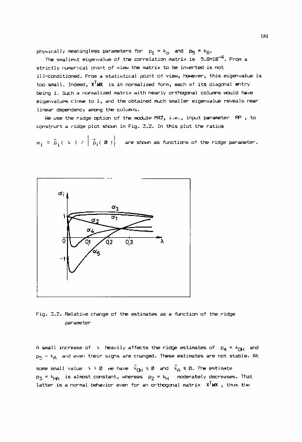
181

physically meaningless parameters for p1 = ko and p5 = kp. The smallest eigenvalue of the correlation matrix is 5.8~10)-~. From a

strictly numerical point of view the matrix to be inverted is not

ill-conditioned. From a statistical point of view, b v e r , this eigenvalue is

t w small. Indeed, XTWX

being 1. Such a normalized matrix with nearly orthogonal c o l m s wwld have

eigenvalues close to 1, and the obtained much smaller eigenvalue reveals near

linear dependency among the colums.

is in normalized form, each of its diagonal entry

We use the ridge option of the module M42, i.e., inprt parameter Rp , to construct a ridge plot shown in Fig. 3.2. In this plot the ratios

ai = ^pi( X ) / I p̂i( B ) I are shown as functions of the ridge parameter.

I “;t I Qa

Fig. 3.2. Relative change of the estimates as a function of the ridge

parameter

A small increase of x heavily affects the ridge estimates of p4 = kw and

p5 = kA and even their signs are changed. These estimates are not stable. At

s m small value X > 0 we have cw 5 0 and 2, 5 0. The estimate

p3 = kHFI is almost constant, whereas p2 = kH mderately decreases. That

latter is a normal behavior even for an orthogonal matrix X’WX , thus the

182

,-. estimate of kH is also stable. The estimate p1 = ko changes in an

interesting way. While

and remains almost constant further on. Thus this parameter estimate is

evmtually stable, but can be neglected because of its small value. Chr

analysis supports the assumption that the reaction i5 acid-catalysed with the

only essential parameters kH and kHA considered in model (3.64).

* pl( 0 ) is negative, it changes sign at a m a 1 1 x > 0

The information revealed by ridge plots as the m e shown in Fig. 3.2 can

be better understood noting that the ridge estimate (3.63) is the solution of

the minimization problem:

IIpII --> min ,

where C > 0 i5 an increasing function of X (ref. 23) . Therefore, an elongated confidence ellipsoid results in wildly changing ridge estimates for

some of the parameters, whereas other parameters remain stable.

subject to the constraint Q(p) - Q(p(0) ) = C ,

3.5.2 Overparameterized nonlinear models

On the basis of it5 constrained minimization interpretation the ridge

regression technique can be extended to nonlinear models, but the construction

of ridge plots requires considerable computing effort. Therefore, ridge

regression is rarely used in nonlinear estimation, though near singularity is

an even m r e inherent problem than in the linear case. In fact, the small

eigenvalues of the cross product matrix

increased by appropriate experiment design (see Section 3.10.21, the

eigenvalues of the matrix JT(0)WJ(O)

also on the form of the response function and the actual parameter values.

Therefore, the psibilities of eliminating near singularity by experiment

design are usually quite restricted in the nonlinear case. For example, the

partial derivatives of the Arrhenius function (3.49) are ak/W = exp[-E/(RT)l

and ak/& = - A expC-E/(RT)l/(RT), and the columns of the Jacobian matrix are

nearly collinear if the rate constants are observed over a relatively small

temperature intervall, as usually restricted by the experimntal techniques. In

such cases the model might be overparameterized (see, e.g., ref. 24) in spite

of its apparent simplicity.

eigenvalue-eigenvector analysis. In the module M45 the matrix JT(0)WJ(Li)

is investigated. We call it normalized cross product matrix, because the

partial derivatives are computed with respect to the normalized parameters

X ’ W X of a linear mdel can be

of a nonlinear &el depend, haYever,

Overparameterization and frequently its sources are revealed by an

183

p - = p . / ~ . ( ~ ) . In cmtrast to the linear case, this matrix is not normalized further to a correlation type matrix before the principal component analysis.

Its eigenvalues and eigenvectors are of considerable help when interpreting the

results. For example, at most 107. relative mean error in the parameters

implies the inequality

normalized parameters in JT(p)WJ(p) and according to (3.62) , this can be

attained if the smallest eigenvalue satisfies the inequality

J J J

E{ CP - 31T[p - 31 1 < 0.01 . h e to the use of

> la^ 2 z IDZ 2 , where s2 is the estimate of the squared sigma factor

in the weights. 6s usual, we consider the estimation problem nearly singular if

the smallest eigenvalue is below this limit.

Another advantage of the normalized parameters is that the eigenvectors

corresponding to small eigenvalues frequently reveal the form of nonlinear

dependences a m g the estimates. For this interpretation we introduce the

parameters

have

aj = log c pj I. It is important to note that at p = p(k) we

af/apj = af/aaj = (af/ap.)p.(k) , and hence the two parameter J J transformations w e introduced locally give the same Jacobian matrix.

Furthermore, we exploit the canonical form

(3.65)

h h

of the quadratic approximation (3.42), where

Afi = uiT[ a - 3 . Moving from the point a along the eigenvector ui

by a step of unit length implies

?J ( a ) - O( a ) z xi. Assume that eigenvector is

we move along ui, and a ( a ) - a ( ) Z 0 . The line Aal = Aa2 in

the space of the a’s corresponds to the curve log[ pl/@ I = log[ p1/p2 I , i.e., p1/p2 = const., in the space of the original parameters. Thus, keeping

the ratio p1/p2

In other mrds the objective function depends only on the ratio

does not depend on the individual parameters p1 and p - ~ separately.

Similarly, the eigenvector

a nearly zero eigenvalue xi m the product

Corresponding to a nearly zero eigenvalue. Then the parameter corresponding to

the coefficient 1 in the eigenvector cannot be identified. The analysis can

also be extended to find relationships -g several parameters, and is

particularly useful in chemical kinetics (ref. 25-26).

aj = log C pj 1 and

h

(Afi)’ = 1, (Afj)2 = 0 for ifj, and hence

r A

xi 5 0, and the corresponding

ui = [0.707, 0.707, 0, ..., 0IT. Then selecting &al = Aa2

A h

fixed, the objective functim value r a i n s almost unchanged.

p1/p2 , and

ui = C0.707, -0.707, 0, ..., 0IT corresponding to

reveals that the objective function depends only

p1p2. It is even simpler to interpret a unit vector

184

Exercise

0 At a fixed value V = 0.035~10-’ mol/(l s) and several values of K between

lK3 ml/l and

(3.55) at the substrate concentrations listed in Table 3.4. Perform principal

component analysis (using the module M45 and setting IM = 1) of the

normalized crc155 product matrix. Find a value

only the parameter V can be estimated with reasonable accuracy.

Similarly, find K2 such that if K > K2 then a reasonable estimate can

be obtained only for the ratio

0.1 moll1 , compute the error-free rates from the model

Ki of K such that for K < K1

V/K.

3.6 MJ-TIRESWNSE ESTIMATION

In Section 3.3 we a l l 4 the errors in the observatims qil, ;iz, . . . , qi,ny to te correlated, tmt apart from a scalar factor a2 their covariance

matrix was asKlmed to be k n w . The rmltiresponse estimation method proposed by

Box and Draper (ref. 27) does not require this strong assumption. The method

is based m the maxim likelihood principle, and involves the minimization of

the objective function

O ( p ) = detC V(p) 1 (3.36)

where

(3.67)

is the nymy empirical covariance matrix cunputed at the actual parameter

vector p . Notice that the errors in different sample points are still assumed to be uncorrelated. The determinant criterim (3.66) is equivalent to the

unweighted least squares method if mly one dependent variable is observed in

every sample point. For the rmltiresponse case it is, at least from a

theoretical point of view, a more general estimator than the least squares.

Lhfortunately, there are sure technical difficulties associated with the

determinant criterim (ref. 28). Minimizing the determinant (3.66) is not a

trivial task. In addition, the method obviously does not apply if detC V(p) 1

is zero or nearly zero for all parameter values. This is the case if there

exist affine linear relationships ammg the respmses yl, y2, ..., Yny~ as we

dixussed in Section 1.8.7. To overcome this problem the principal component

analysis of the observations is applied before the estimation step.

185

Example 3.6 Compariscn of the determinant criterion wi th least s q u a r e s

Return to the example of Box et a l . ( r e f . 29) we s t a r t e d to d i s c u s s i n

Sec t ion 1.8.7. The thermal i somer i za t ion be desc r ibed by t h e mechanism show,

i n F igu re 3.3.

F ig 3.3. Mechanism of the thermal i s o m r i z a t i o n of a-pinene

Assuming f i r s t o r d e r reactions, the mechanism g i v e s rise to a set of f i r s t

o r d e r d i f f e r e n t i a l equat ions. T h e fol lowing s o l u t i o n of t h e equa t ions g i v e s the

component concen t r a t ions yl, y2, ..., y5 as func t ion o f t h e reaction t ime t:

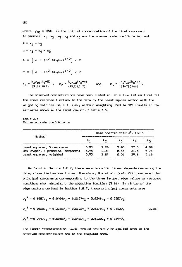
186

where y10 = lC0L

(a-pinene); kl, k2, k3, k4 and kg are the unknow, ra te coefficients, and

i s the i n i t i a l concentration of the f i r s t component

5 = kl + k2

a = k3 + k4 + k5

P = [-a + / 2

7 = [-a - ( r ~ ~ - 4 k ~ k ~ ) ~ / ~ ] / 2

The observed concentrations have been l i s ted i n Table 1.3. Let us f i r s t f i t

the above response function to the data by the least sqares method with the

weighting matrices

estimates shown i n the f i r s t row o f of Table 3.5.

Wi = I , i.e., without weighting. M u l e M45 results i n the

Table 3.5 Estimated rate coeff ic ients

As found i n Section 1.8.7, there were two a f f i n l inear dependences m g the

data, c lassi f ied as exact ones. Therefore, Box e t a l . ( re f . 29) considered the

principal components corresponding to the three largest eigenvalues as response

functions when minimizing the objective function (3.66). By v i r tue o f the

eigenvectors derived i n Section 1.8.7, these pr incipal comments are:

(3.68)

The linear transformation (3.68) should obvicxlsly be applied both t o the

observed ccncentrations and t o the computed ones.

187

0.745 -0.269 -0.234 -0.016 -0.250l

-0.269 0.715 -0.247 0.018 -0.264

-0.234 -0.247 0.785 -0.- -0.230

-0.016 0.018 -0.m 0.001 0.005

-0.258 -0.264 -0.230 0.005 0.755

Based on the analytical expression for the derivative of detC Wp) 3 , Bates and Watts (ref. 30) recently proposed a Gauss-Newton type procedure for

minimizing the objective function (3.66). We use here, howwer, the simplex

methad of Nelder and Mead (module My)) which is certainly less efficient but

does not require further programing. The determinant is evaluated by the

module M14. After 95 iterations we obtain the results shum in the second row

of Table 3.5, in good agreement with the estimates of Box et al. (ref. 29 1.

Canparing the first and second rows of Table 3.5 we could cmclude that the

least squares and the determinant criterion yield significantly deviating

estimates. This cmclusion is, however, not completely true. We repeat the

estimation by the least squares method, but considering the three principal

components (3.68) as responses. This can alternatively done retaining the

original model with five responses, but introducing the weighting matrix

elements

with

where uik is the i-th element of the k-th eigenvector compted in Section

1.8.7. Then the nondiagmal weighting matrix

W =

is used in the d u l e M45, exploiting the weighting option WI = 2 . The result of the estimatim is shcw, in the third row of Table 3.5.

Cansidering the recent general dislike of statisticians t w r d the

application of the least squares method to rmltiresponse problms, it is

surprising to =ee that having eliminated the linear dependences from the data,

the least squares method gives very similar estimates to the determinant

criterion. Thus, in this f a m s example a preliminary screening of the data is

rrure important than the choice of the estimation criterion. To put it more

simply, the analysis of linear dependences revealed that had not been

measured but assumed, thwgh its values significantly influenced the estimate

of k3, in accordance with the reaction mechanism shown in Fig. 3.3. Using

three principal canponmts we practically dropped these "measurements", and

obtained an improved value of

criterion.

y4

k3, a l m t independently of the estimation

188

3.7 EUJILIBRATIffi R F W C E EWTIONS

The problem to be solved here primarily cmes from chemical engineering

where m e sirmltanwusly observes several variables that are expected to

satisfy a number of balance equations such as stoichiometric relations. Due to

measurement errors the observed values obviously do not fulfill this

expectation. Let xl, xz, ..., xnv denote these variables observed in a single

sample point that gives the data { xi = xi + Ci; i=l,nv 1. CkKtming that the

covariance matrix c o v { C ) = V of the error vector C is diagonal and knum,

we would like to find the values x that minimize the quadratic form

c

cx - ;IT v-1 cx - ;I

and, at the - time, satisfy the set W x - b = 0

(3.69)

(3.70)

of nb linear balance equations. Since we do not have unknown parameters, and

observe the variables only once, this problem differs from the ones studied in

the previous sections. Nevertheless, the same estimation tecbique is used and

the results will be useful for parameter estimation in the next section.

c Introducing the correction vector c = x - x and the equation error vector

*.

f = Wx - b, according to (3.69) and (3.70) we minimize the objective function

Q(c) = cT V1 c (3.71)

subject to the constraints

W + f = O . (3.72)

PI similar constrained optimization problem has been solved in Sectim 2.5.4

by the method of Lagrange mltipliers. king the same method we look for the

stationary point of the Lagrange function

L ( C , X ) = CT v-1 c + AT c w + f 1 (3.73)

where denotes the nb-vector of Lagrange rmltipliers. At the stationary

point the partial derivatives of the function (3.73) vanish

a ac - = 2 2 1 c + w T x = 0 , (3.74)

(3.75) a -- = K + f = 0 . ax

189

l3y

X = 2CWI-lf , and using (3.74) c = - (1/2)WJTx . Introducing this value into (3.751 gives

(3.74) again, we obtain the optimal correction

c = - WJTCWTI-lf . (3.76)

Thus the problem can be analytically solved, similarly to linear regression. At

the correction (3.76) the objective function (3.71) takes the value

q2 = fTCwTl-lf , (3.77)

called error measure in the literature of balance equilibration.

The error measure is invariant under rexaling the equations (3.70) and even

under replacing the original equations by their independent linear

cmbinatims. This latter m y be necessary if the matrix is singular and

hence the inverse in (3.77) is not defined. Since V ir a diagonal matrix with

nonzero diagonal entries, this case reveals that the balance equations are not

linearly independent. The problem can be resolved by considering a m a x i m

linearly independent subset of the balance equations.

WT

Since qz is distributed as X2 , the measuremnts can be accepted if

(3.78)

where the right hand side is the tabular value of the

nb degrees of freedom at the significance level a, usually at a = 0.05 . Unfortunately, the error variances should be exactly known for this test. If

the error variances are known only up to a scalar factor, then the correction

vector is still correctly givm by (3.76) , but the inequality (3.78) is of

no value.

X2 distribution with

Nevertheless, if (3.78) is known to be violated, a further issue is to

find the variable that is primarily responsible for the violation. The ratio of

the absolute value of the correction to the corresponding standard deviation

provides s ~ e information but may be misleading (ref. 31) . The analysis proposed by Almdsy and Sztanb (ref. 32) is based on geanetric ideas. If

exactly one observation is corrupted by gross error then the corresponding

colurm of matrix W and the vector f of equation errors are nearly

collinear. Useful measures of collinearity are 7i = cos ai , where ai is the

angle bet- f and the i-th c o l m of W . The variable suspected to be corrupted significantly is then the one corresponding to the largest AlmAsy

indicator 17i 1 . The Ti values are invariant under scaling of the balance

equations (ref. 32) .

190

Proqram d u l e M 5 0

5000 HEM ~ t l l l t t t t t t t t t t t t t t t t t l t t l l l l t l t t t t l t l l t t l t t t ~ l l l l l 500: RE# I EQUILIBRATINS LINEAR BALANCE EOUATIONS PV 1 5004 REH t LEAST SOUARES METHOD AND OUTLIER ANALSSIS t 5006 REM t t I t I t t 1 t t t t t t I t I t I l l t 1 l l t l t l t l l t t I t I t I I t t t t f Ill1 I t 5008 BE1 INPUT: 5010 REh NE NUMBER OF BALANCE EQUATIONS 5012 RE\ NV NUMBER OF VARIABLES 5014 2Eti WINB,NVI HEITRIX OF COEFFICIENTS IN EQUATIONS 51lb REN B!NBJ RIGHT HAND SIDE OF EQUATIONS 5%13 RE! X(NV) OBSERVATIONS 5620 REN V(NV1 VARIaNCES [SQUARED ERRORS) OF VARIABLES 5122 RE1 OUTPUT: 5024 REK EE STRTUS FLAG 5026 REM 0 SUCCESSFUL EQUILIBRATIDN 5128 REM 1 LINEARLY DEPENDENT EQUATIONS 5838 RE\ FINPI EQUATION ERRORS BEFORE EOUILIBRATING 5632 RER C(NV) CORRECTIONS OF VARIIBLES

5136 RER BINV) VECTOR OF ALIASY I I IDICATORS 5038 REfl CH 5048 REM AUXILIARY ARRAYS: 5042 REH A(NB,NR),T(NV,NRl 5844 RE1 b@DULE CALLED: Nib 504t ~ E H ---------- T.VIJ' 5048 FOR 1-1 TO NV :FOR J-1 TO N B 5850 T I I , J)=W( J , I ltV( I I 5052 NEXT J :NEXT I

5E5b FOR 1.1 TO NB :FOR J=l TO I 5858 A=O :FOR K=l TO NV :A=AtWII,K)tT(K,J) :NEXT K :A(I,J)=A 5060 NEXT J :NEXT 1

5064 N=NB :GOSUB I600 :IF ER=I THEN 5128

50b8 FOR 1.1 TO NB 58'0 5872 NEXT I 50!4 REH ---------- (WVW )'-ltF 5076 FOR 1=1 TO NB 5078 T.0 :FOR K = l TO NB :T=T+B(I,KltF(K) :NEXT R :T[I,I)=T 5880 NElT I 5882 RE!! ---------- COlfPUTE CORRECTIONS 5084 FOR 1.1 TO NV 5186 5088 NEXT I

SUH OF SQUARES 5898 RE! __-_-_____ 5892 QN :FOR 1.1 TO NB :Q2=02+FII)tTIB,I) :NEXT 1 :D=SQR(02)

5896 FOR 1.1 TD tiV :FOR J=! TO NB 5098 T.0 :FOR Y=l TO NB :T=T+W(K,IllRlk',J) :NEXT K :TII,J)=T 5iB0 NEXT J :NEWT I 5102 REM ---------- 61 I l=(llq) (DIAStw' IWVU' i'-ltWlA-0.5)tW' ( W V W ' lA-ltF

5034 REH 02 WEIGHTED sun OF SOUARES OF CORRECTIONS

CH! SQUARE A T 8.05 SIGNIFICANCE LEVEL IIF NB<=lI)

5854 REN ---------- A=WVY'

P=( UVW' 1 '-1 5062 RE! __--------

$066 REn ___--_____ F

Fz-BII! :FOR k'=I TO NV :F=FtW(I,R)tX(K) :NEXT K :F(I)=F

C=R :FOR K.1 TO NB :C=C-TII,K)tT(0,I() :NEXT k :C(I)=r

5094 RE! ---------- T=W'(WV#']"-1

5184 FOR 1=1 TO NV 5106 D=$ :E=8 5188 FOR I 4 T O Nb 5110 D=DtT( I , K l lU(K, I ) :E=EtTI I ,K) tF(ll1 5112 NEXT t!

191

5114 G(I)=liQ/SQR(C)lE 5116 NEXT I 5113 REM ---------- CHI SQURRE 5 1 3 CH=Q :IF W10 THEH 5126 5122 CH= - ( N H = I ! ~ L B ~ - ( N P = : ) lS,99-iNB=3! 17.81-(NB=4)19.49-( NB=S)tll. 1

5126 ER=E

5130 HER l l l t t t l l l l l l t l l t l t l l t t t t l t l t l t l l l l l l l l ~ t l t l l l l l

5124 C H ~ C H - ( ~ P ~ 6 ) 1 1 ~ . ~ - ( M B . i ) t ! 4 . i - ( N P . B ) t l 5 . S ~ ( N B ~ 9 ) 1 1 6 . 9 - ( N P ~ 1 0 ) t 1 ~ . 3

size RETURN

Since the covariance matrix is diagmal, a vector denoted by V is used to

store the variances. If the number of balances does not exceed ten, the module

also computes the tabular value of the chi square distribution at significance

level a = 0.05 and degrees of freedom nb. The return value ER = 1 of the

status flag indicates that the rcws of the matrix W are linearly deplndent,

and hence you should drop at least one of the balance equations. If the source

of linear dependence is not clear then the module Ml0 can help to uncover it.

Example 3.7 Equilibrating linear balance equations

The four variables x1, xz, XJ, and x4 describing a process are expected

to satisfy the balance equations (ref. 31):

0 . 1 ~ ~ + 0.6~~ + - 8.2~~ - 0.7~~ = 0

0.8x1 + O.lxz + - 0.2x3 - 0.1x4 = 0

0.1~1 + 0.3~2 + - 0.6~3 - 0.2~4 = 0 .

The observations and error variances are s k w in Table 3.6.

Table 3.6 Observed values and variances for the balance equilibration problem

variable measured variance

x1 0.1858 0.002mP

x4 3.eEam O.m

x2 4.7935 0.IDZP5 x3 1.2295 0.000576

The main program and the results are as follows:

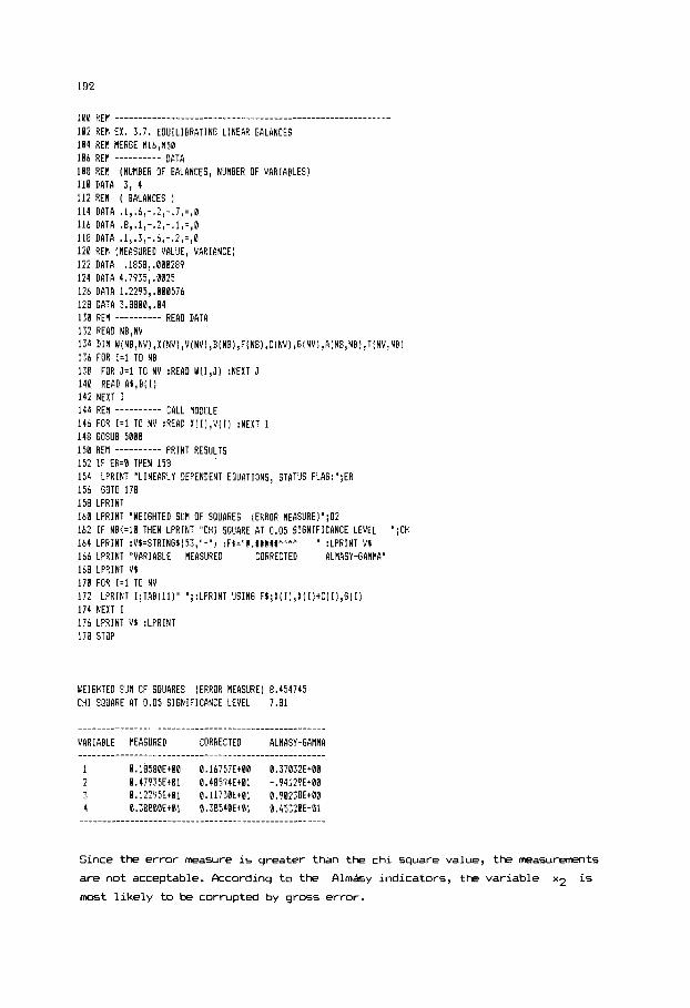
192

180 HEN ........................................................... 182 REM EX. 3.7. EQUILlERATING LINEAR EALANCES 104 HEN IIERGE N16,N51

118 RE1 110 DATA 3 , 4 112 REM ( EALRNCES )

114 DATA .1,,5,-,2,-.7t=,1 115 DATA .8, .1,-.2!-,1,=,1 118 DATA .l , .3,-.6,-. 2 , = , 0 120 RE! (MEASURED VALUE, VARIANCE) 122 DATA ,1858, ,001289 124 DATA 4.7935,.0125 125 DRlR 1.2295, .000576 128 DATA 3.8800,.14 130 REH ---------- READ DATA 132 READ NP,NV 134 DIM W lNR,NV), X lNV1 , V( NS) R INRI ,Fl NF) ,C ( NS) ,G(NV) , A ( NE,NPI ,TI NV,NE 135 FOR 1.1 TO NB 138 FOR J=l TO NV :READ U(I,Jl :NEXT J 146 READ AI,P(I) 142 NEXT I 114 RE! ---------- CALL HODULE 145 FOR 1.1 TO NS :READ XlI),V(I) :NEXT I 148 GOSUR 5001

PRINT RESULTS 152 IF EFi.0 THEN 158 154 LPRINT 'LINEARLY DEPENDENT EQUATIONS, STATUS FLA6:";ER 156 GOTO 178 158 LPRINT 150 LPRINT "WEIGHTED SUH OF SOUARES [ERROR NEASURE:';Q2 162 IF NP<=l8 THEN LPRIRT "CHI SQUARE AT 0.05 SIGNIFICANCE LEVEL 164 LPRINT : V$=STRINGI [53! "-I ) :F$='#. # # # l X * " " " 156 LPRINT "SARIAPLE HEASURED CORRECTED ALNASY-GAflMAu 168 ?PRINT V$ I71 FOR 1.1 TO BV 172 LPfiIRT I;TAP(11)" ";:LPRINT KING F$;X[I) ,K(l)tC(I),G[I! 174 NEXT I 176 LPPINT Vb :LPRINT 178 STOP

116 REN ---------- DATA (NUNPER OF BALANCES, NUNPER OF SARIAPLES!

158 RE4 _ _ _ _ _ _ _ _ _ _

';CH :LPRINT V$

YEIGHTED SLIH OF SQUARES CHI SQUARE AT 0.05 SIGNIFICANCE LEVEL 7.81

(ERROR PlEkSURE) 8.454745

Since the error measure i s greater than the ch i square value, the measurements

are not acceptable. According t o the CllmAsy indicators, the variable x2 i s

most l i k e l y t o be corrupted by gross error.

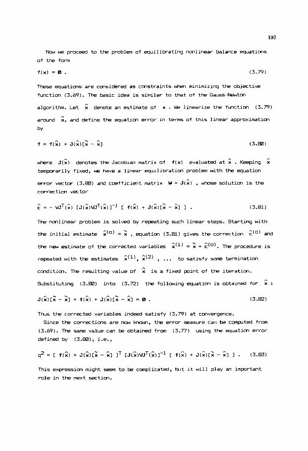
193

Now we proceed to the problem of equilibrating nonlinear balance equations

of the form

f(x) = 0 . (3.79)

These equations are considered a5 constraints when minimizing the objective

function (3.69). The basic idea is similar to that of the Gauss-Newton

algorithm. Let x denote an estimate of x . We linearize the function (3.79)

arowd x, and define the equation error in terms of this linear approximation

A

h

by

h

where J(C) denotes the Jacobian matrix of f(x) evaluated at . Keeping x

temporarily fixed, w e have a linear equilibration problem with the equation

error vector (3.80) and coefficient matrix

correction vector

W = J(C) , whose solution is the

The nonlinear problem is solved by repeating such linear steps. Starting with

the initial estimate

the new estimate of the corrected variables

repeated with the estimates ;(I), ;(') , ... to satisfy 5ome termination

condition. The resulting value of x is a fixed point of the iteration.

Substituting (3 .80) into (3.72) the following equation is obtained for x :

;(O) = z , equation (3.81) gives the correction ;(O) and

= + ;(O). The procedure is

h

h

Thus the corrected variables indeed satisfy (3.79) at convergence.

Since the corrections are now known, the error measure can be computed from

(3.69). The same value can be obtained from (3.77) using the equation error

defined by (3.801, i.e.,

This expression might seem to be complicated, but it will play an important

role in the next section.

194

3.6 FITTING ERROR-IN-VARIABLES M l D a S

If the assumption of neglecting errors in independent variables cannot be

justified, there is no statistical distinction bet- dependent and

independent variables. Then we rather use the vector

denote the variables of the model written in the more general implicit form

z = (z~,z~,...,z~~)~ to

f(z,p) = 0 . (3.84)

The model consists of nk equations and contains np unknown parameters p

to be estimated f r m nm observations. The outcane of the i-th observation

is the data vector

allow for sane error Cij in all variables.

errors in the i-th observation can be correlated, their covariance matrix Vi

is assumed to be know, i.e.,

E{ ci > = 0, EC GiGiT 1 = Vi

- * - .% -.. zi = (zil,zi2 ,..., ~ i , ~ ~ ) ~ where z . - = z - - + L... Thus we

1J 1J 1J

We assume that errors in different observations are uncorrelated. Although

and E{ GiGjT 1 = 0 if i f j . (3.65)

In order to obtain the parameter estimates

21 = (Zil, zi2, ..., zi,nz)T, i = 1 ,..., nm, ttw error norm function ^p and the corrected variables

h h h h

(3.86)

h

is minimized with respect to zi's and p , subject to the constraints

h

f(zi; p) = 0 , i = 1, 2, ..., nm . (3.87)

The above criterion can be derived f r m the maximum likelihood principle

(refs. 33-34).

Having a well defined minimization problem, we can proceed to its solution.

At any fixed p minimization of (3.66) subject to (3.67) is equivalent to

solving nm nonlinear balance equilibration problw of the form

(3.88) h

f(zi; p) = 0 .

Solving the nonlinear balance equilibration problems (3.88) and cmplting the

error measures frcm (3.63) we obtain

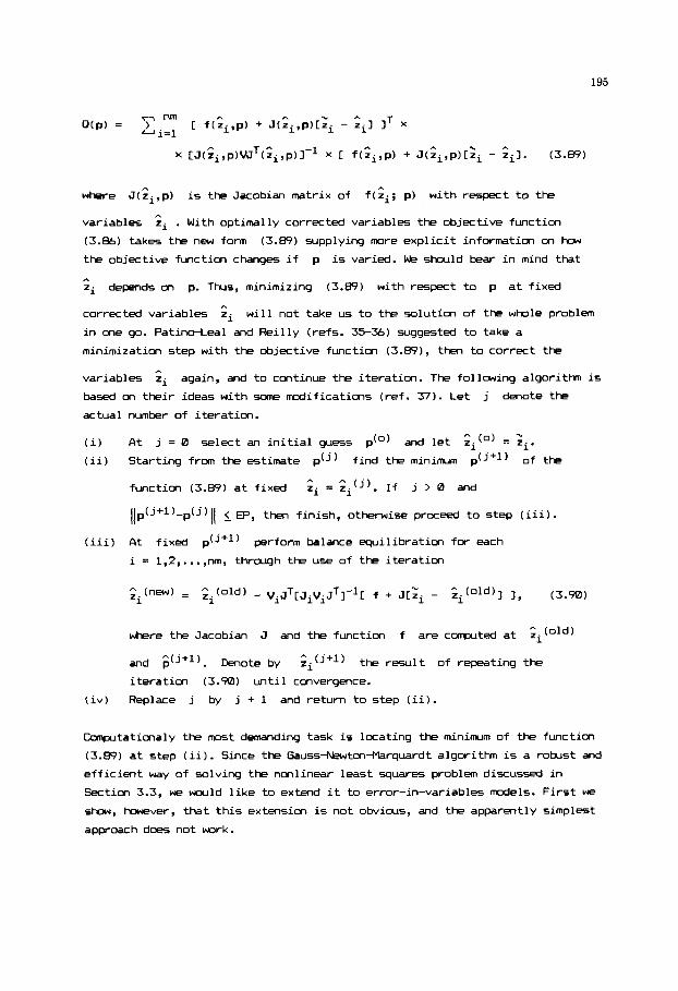
195

h h h h - , A

X [J(~~,p)VJ~(z~,p)l-~ x C f(zi,p) + J(zj,p)Czi - zil. (3.89)

h h

where J(zi,p) is the Jacobian matrix of f(zi; p) with respect to the

variables

(3.86) takes the new form (3.89) supplying mre explicit information on how

the objective function changes if p is varied. W e should bear in mind that

zi depends on p. Thus, minimizing (3.89) with respect to p at fixed

corrected variables zi

in one go. Patindeal and Reilly (refs. 35-36) suggested to take a

minimization step with the objective function (3 .89) , then to correct the

variables zi

based on their ideas with some modifications (ref. 37). Let j denote the

actual number of iteration.

(i) At j = 0 select an initial guess p(O) and let ;i(o) = zi.

(ii) Starting from the estimate p(J) find the minim p(J+') of the

h

zi . With optimally corrected variables the objective function

h

h

will not take us to the solution of the whole problem

h

again, and to continue the iteration. The following algorithm is

-.,

h

function (3 .89) at fixed zi = ;i(J). If j > 0 and

[lp(J+')-p(J)ll < EF', then finish, otherwise proceed to step (iii).

(iii) At fixed p(J+') perform balance equilibration for each

i = 1,2, ..., nrn, through the use of the iteration

where the Jacobian J and the function f are computed at ;i(old)

and G(J+'). Denote by si(J+') the result of repeating the

iteration (3.90) until convergence.

(iv) Replace j by j + 1 and return to step (ii).

Computationaly the most demanding task is locating the minimm of the function

(3 .89) at step (ii). Since the Gauss-Newton-Marquardt algorith is a robust and

efficient way of solving the nonlinear least squares problem discussed in

Section 3.3, we would like to extend it to error-in-variables models. First we

show, however, that this extension is not obvious, and the apparently simplest

approach does not work.

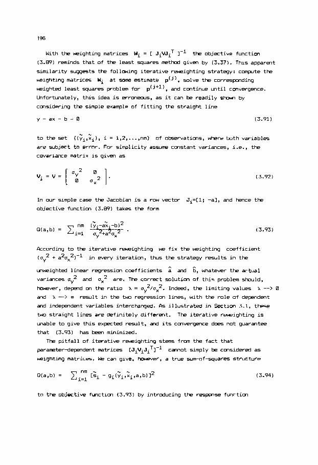
196

With the weighting matrices Wi = C J.VJ.T I-' the objective function 1 1

(3.891 reminds that of the least quares method given by (3.37). This apparent

similarity suggests the following iterative reweighting strategy: compute the

weighting matrices Wi at 5ome estimate p(j), solve the corresponding

weighted least squares problem for

Lhfortunately, this idea is erronwus, as it can be readily show, by

considering the simple example of fitting the straight line

y - a x - b = 0 (3.91)

p(J+l), and continue until convergence.

* * to the set {(yi,xi), i = 1,2, ..., nm} of observations, where both variables

are subject to error. For simplicity assume constant variances, i.e., the

covariance matrix is given as

(3.92)

In our simple case the Jacobian is a row vector

objective function (3.89) takes the form

Ji=C1; -a], and hence the

kcording to the

'uy2 + a2ux2r1

(3.93)

iterative reweighting we fix the weighting coefficient

in every iteration, thus the strategy results in the

h h

unweighted linear regression coefficients a and b, whatever the actual

variances (3 and ux2 are. The correct solution of this problm should,

however, depend on the ratio

and X --> rn result in the two regression lines, with the role of dependent

and independent variables interchanged. As illustrated in Section 3.1, these

two straight lines are definitely different. The iterative reweighting is

unable to give this expected result, and its convergence does not guarantee

that (3.93) has been minimized.

parameter-dependent matrices CJiViJiT]-' cannot simply be considered as

weighting matrices. We can give, however, a true Kim-of-squares structure

Y X = u 2/ux2. Indeed, the limiting values A --> 0 Y

The pitfall of iterative reweighting stem f r m the fact that

to the objective function (3.93) by introducing the response function

197

(3.95)

I

and the "observed" responses si E 0 for all i = 1,2,...,nm. Since

minimization of (3.4) is now equivalent to solving a nonlinear unweighted least

squares problem, the Gauss-Newton-Marquardt procedure applies. We note that for

this simple illustrative problem we do not really need the iteration procedure,

since there exist explicit expressions for the error-in-variables estimates of

a and b, see (ref. 1). The idea of incorporating the induced weights into the

response function is, b v e r , generally applicable and requires the

decompcsi tion

c J~(P)vJ~~(P) I-1 = Q~~(P)Q~(P) , (3.96)

thereby transforming the objective function (3 .89) to the unweighted sum of

squares form

(3.97)

h

where si P 0 for all i = 1,2,...,nm. Since in step (ii) of the

error-in-variables algorithm zi is fixed, we omitted it from the

arguments of Qir fi and Ji. When minimizing (3.97) we can use a nonlinear

least squares algorithm with the nk-dimensional virtual response function

defined by

h

for the i-th observation.

If the problem is multifunctional, i.e., nk > 1 , then the decomposition (3.96) is not unique. It is advisible to use the Cholesky decomposition

c J.v.J-T 1 1 1 1 = L ~ L ~ ~ where L~ is a lower triangular matrix. TM oi = ~ ~ - 1 is

a suitable matrix satisfying (3.96). Efficient algorithms for obtaining Li

and then Qi

Lines 5404 through 5436 of the following module are based on their

algorithmic ideas.

can be found in the book of Wilkinsm and Reinxh (ref. 38).

The organization of the module is sonwhat tricky in order to make use of the

nonlinear least squares module M45. Indeed, the module M52 is essentially a

server subroutine for the module M45.

198

Prwram module M52

5208 REM t t t t t t t t l t t t t ~ t t t t t t ~ t t t l t l t l ~ t l l t t t t t t t t t t t t t t l l l t 5202 REH t F I T T I N G AN ERROR-IN-VARIABLES HODEL 1 5284 RE1 1 OF THE FORM F ( z , r ) = e t 5286 REW t RODIFIED PATINO-LEAL - REILLY HETHOD 1 5208 RE! t t t t t t t 1 1 11 1 1 t t It t t l t t t t t t t t t t 11 t t t 1 t t i t t t t t t t t t t t t 5 2 1 8 REh INPUT: 5212 RE! NM NUMBER OF SAHPLE POINTS 5214 REH tJZ NUHBER OF VARIABLES 5 2 1 6 REM N I NUBBER OF EQUATIONS 5218 REH NP NUMBER OF PARMETERS 5220 RE1 T[NH,I...NI) TABLE OF OBSERVATIONS 5222 RER R ( N 2 ) VARIANCES OF VARIAELES 5224 REH P(NP) I N I T I A L PARAHETER ESTIMATES 5226 REH EP THRESHOLD ON RELATIVE STEP LENGTH OF PARAilETERS 5228 REI! EZ THRESHOLD ON STEP LENGTH OF VARIABLES 5238 REH I M MAXIHUR NUHBER OF ITEPATIONS

5234 RE! ER STATUS FLbG 5236 REil B SUCCESSFUL ESTIMATION 5238 REH 1 THRESHOLDS NOT ATTAINED 5240 HE\ 2 HRTRIX Fz'lRlFz ND7 PDSlllVE D E F I N I T E 5242 RER ( LOCALLY DEPENDENT EQUATIONS ) 5244 REM P(NP) PARAMETER ESTIMATES 5246 HEM T(NM,N!+!,. .21N2) CORRECTED VARIABLES 5248 REH ... .. FURTHER RESULTS PRINTED I N THE HODULE 5250 REH USER-SUPPLIED SUBROUTINES: 5252 REH 5254 RER GOSUB 5399 :RETURN 5256 REN FRO\ L I N E 788: 5258 REH 5260 RER 5262 REH FROH L I N E 60s: 5264 REB 9266 REW 5268 REM AUXILIARY ARRAYS: 5278 REM A(NP,NP) ,CiNP, NP ,U(NP,NP) , X 121N2 ) ,Y (NK) ,B(NP) ,D ( NP ) ,S(NP) ,6 ( NK ,NP 5272 RER V(NM ,NK) ,RINK ,NK ) , H ( N I ,NK 1, W (NK , NK) 5274 REM MODULES CALLED: ti l6,Hlfl,H41,H45 5276 NX=NLtNZ :NY=NK : M I 4

$232 REN m u T :

FROM L I N E 988; OBLIGATORY STATEIlENTS ARE

Z(1. I .nz) ,P( l . . .np) ---) Fll ... n k ) ( FUNCTION VALUE EVALUATION )

2 (1. I . n z ) ,P( l . . .np) ---) E(1. . .nk ,1,, a nz 1 ( P l R T l A L DERIVATIVES OF F H I T H RESPECT TO I )

5278 REIl ---------- I N I T I A L ESTIMATE OF VARIABLES 5 ~ 8 0 FOR H=I TO Nti

5286 NEIT t i

5282 FOR 1 = 1 TO NZ : T ( M , N Z + l ) = T i t i , I ) :NEXT I 5284 FOR 1.1 TO NY :V(M,I)=8 :NEXT I

5288 FOR 16.1 TO I H 5290 LPRINT :LPRINT T A B ( 1 5 ) ; " t t t t t l k U k NONLINEAR LSQ ESTIRRTION "; 5292 LPRINT "NUNBER'jIG;' t l l t t t t t t t " ; LPRINT 5294 FOR 1.1 TO NP : S ( I ) = P ( I ) :NEXT I :GOSUB 4580 5296 IF ER:0 THEN 5448 5298 LPRINT :LPRIWT TAB(15);"tttttttttt CORRECTED VARIRBLES t l t t t l l l t t '

5382 FOR M = l TO N I 5384 FOP 11-1 TO Iil 5386 ZE.0 5318 FOR 1.1 TO NX : X ( I ) = T ( H , l ) :NEXT I 5310 GOSUB 537E

5388 LPRINT PRINT

199

5312 FOR I=1 TO NK 5314 V=B :FOR J=l TO NK :V=YtA(I,J)tFIJ) :NEXT J :VIIl=V 5316 NEXT I 5318 FOR 1.1 TO NZ 5328 Z=X(I) :FOR J.1 TO NK :Z=Z-R(I)tE(J,I)tV(J) :NEWT J 5322 D=Z-T(R,NZtI) :T(#,NZ+I 1-2 :ZE=ZE+DtD 5324 NEXT I 5326 IF SQR(ZE)<=EZ THEN 5332 5328 NEXT I T 5338 ER=l 5332 REH --------- PRINT VARIABLES 5334 IF tOl THEN 5342 5336 LPRINT V1 5338 5348 5342 FOR 1.1 TO NZ 5344 5346 5348 NEXT I 5350 GOSUB 788 5352 5354 NEXT I! 5356 LPRINT V$ :LPRINT 5358 IF ER=l THEN 5446 5360 REH ---------- TERRINATION CONDITION 5362 PE.0 :FOR 1.1 TO NP :PE=PEt(P(I)-S(Ill^2/S(I)*2 :NEXT I 5364 IF SQRIPE)<=EP THEN ER=0 :60TO 544R 5366 NEXT IG 5368 ER=I :60TO 5448 5370 REH ---------- A=(Fz'tRtFzIA-l 5372 6OSUB 5376 :N=NK :GOSUB I680 :IF ER.1 THEN ER.2 5374 RETURN 5376 REH ---------- AzFz'tRtFz AND F=FtFzt(Z-X) 5378 FOR I0:l TO NZ :Z(IB)=X[NZtIB) :NEXT I 0 5388 6OSUB 68B 5382 FOR 18.1 TO NK :FOR J0.l TO I8 5384 A=B :FOR KB=l TO NZ :A=AtR(K0)tE( I f l ,K8)tE(JB,KB) :NEXT K0 :R(IB,J0l=A 5386 NEXT J B :NEXT I8 5388 GOSUB 788 5398 FOR 18.1 TO NK 5392 A=F(I f l ) :FOR J0.l TO NZ :A=AtElI8,J8)t(X(J8)-Z(J8]1 :NEXT J B :F(I0)=A 5394 NEXT I0 5396 RETURN 5396 REM ---------- RESPONSE FUNCTION 5408 GOSUB 5376 :IF NK)l THEN 5484 5482 IF RIl,l)=0 THEN ER.2 :60TO 544b ELSE Q(lll)=SQR(l/~~l,lll :60TO 5438

5486 FOR 10.1 TO NK

LPRINT ' HEAS";TAB( 71;" I';TAB(ll);'Z(I) HEAS";TRBI26);'Zl11 CORR'; LPRINT TAR(40);"EQUATION ERROR AFTER CORRECTIONn :LPRINT V$

IF I=l THEN LPRINT H; LPRINT TAB( 7);I; :LPRINT USING FS;X(I),Z(Il

FOR K = l TO NK :LPRINT TAB(45);'F[';K;*)=';F(K) :NEXT K

5484 RER ---------- ---------- DECORPOSE A INTO HtH' BY CHOLESKY METHOD

5408 FOR Je=i TO 10-1 5418 5412 H( I0,10)=A/H(JB,J01 5414 NEXT JB 5416 5418 IF A i = B THEN ER=2 :GOTO 5446 ELSE H(I0,IB)=SQR(A) 5420 NEXT I0

5424 FOR 10.1 TO NK 5426 Q( 10, I0]=1/H( 18, 18)

A=A(I0,JBl :FOR K0=1 TO JB-1 :A:A-H(I8,KUltH(J8,K8) :NEXT K8

A=A(I8,IB) :FOR YB.1 TO 18-1 :A=A-H(18,68)*2 :NEXT K8

5422 REn _ _ _ _ _ _ _ _ _ _ _______-__ FIND 0'. Hb[-l]

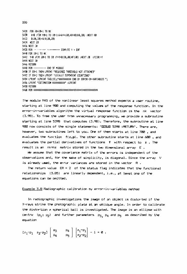
200

5428 FOR JE=iBtl TO NK 5430 A 4 :FOR KB.1 TO JB-l:PI:R-H(J0,KLI)tQ(K0,10~ :NEXT K 0 5432 QiJB,I0)=I1IH(JE,JE) 5434 NEXT J0 5436 NETT I0

5440 FOR 10.1 TO NK 5442 Y.8 :FOR JE=l TO I0 :Y=VtQ(IB,J0)tF(JBI :NEXT J0 :V(IB)=Y 5444 NEXT I0 5446 RETURN 5448 RER ---------- END OF NODULE

5436 REH _ _ _ _ _ _ _ _ _ _ _ _ _ _ _ _ _ _ _ _ COMPUTE Y = QtF

5458 IF ER-1 THEN LPRINT 'REQUIRED THRESHOLD NOT PTTPINED" 545: IF ER.2 THEN LPRINT 'LOCALLY DEPENDENT EQUATIONSn 5454 LPRINT :LPRINT TAB(15);'tttttftttt END OF ERROR-IN-VIRIPBLES "; 5456 LPRINT "ESTIBATION t t t t t t t t t? * :LPRINT 5458 RETURN 5460 PEH t t t t t l t t t t t t t t t t t t t t t t t t t t t t t t t t t t ~ t t t t t t ? j t t t t t t : t

The module M45 of the nonlinear least squares method expects a user routine,

starting at line Saw and computing the values of the response function. In the

error-in-variables algorithm the virtual response function is the nk vector

(3.98). To free the user from unnecessary programming, we provide a subroutine

starting at line 5398 that cmpltes (3.98). Therefore, the subroutine at line

920 now consists of the single statements: "GOSUB 53% :RETLRN". There are,

however, t w o subroutines left to you. h e of them starts at line 7aW , and evaluates the function f ( z , p ) . The other subroutine starts at line UiW , and evaluates the partial derivatives of functions f with respect to z . The result is an nkmz matrix stored in the two dimnsional array E .

We assume that the covariance matrix of the errors is independent of the

observations and, for the sake of simplicity, is diagonal. Since the array V

is already used, the error variances are stored in the vector R . The return value ER = 2 of the status flag indicates that the functional

relationships (3.85) are linearly dependent, i.e., at least one of the

equations can be mitted.

Example 3.8 Radiographic calibration by error-in-variables method

In radiographic investigations the image of an object is distorted if the

X-rays strike the photographic plate at an oblique angle. In order to calibrate

the distortion a

centre (pl; p2)

equation

r

spherical ball is investigated. The image is an ellipse with

and further parameters b, p4 and p5 as described by the

201

h S

The above model is fitted to 20 observed pairs of cmrdinates (ril; zi2) by

Reilly and Patindeal (ref. 35) with the assumption that the errors are

normally distributed and independent with variances

ozz = 0.WZI01 . The following main program contains the observed coordinates in

the DCITA lines

in line 220. Termination criteria for the parameters (Ep) and for the

equalibrated variables (EZ) are given in line 218.

al2 = 0.0001 and

114 - 152 , The initial estimates of the parameters are given

118 REM ........................................................... 182 REM El. 3.8. ERROR-IN-VARIABLES PARAMETER ESTIMATION - CALIBRATION 184 REA HERGE M16,M18,H41,M45,M52 I 0 6 REk ---------- DATA 188 REM (NUABER OF SAMPLE POINTS) 118 DATA 28 112 REM (21, 2'2 114 DATA 0.58, -0.12 116 DATA 1.20, -0.60 118 DATA 1.68, -1.88 128 DATA 1.86, -1.48 122 DATA 2.12, -2.54 124 DATA 2.36, -3.36 126 DATA 2,44, -4.88 128 DATA 2.36, -4.75 138 DATA 2.86, -5.25 132 DATA 1.74, -5.64 134 DATA 1.34, -5.97 136 DATA 0.90, -6.32 138 DATA -8.28, -6.44 140 DATA -0.78, -6.44 142 DATA -1.36, -6.41 144 DATA -1.98, -6.25 146 DATA -2.58, -5.88 148 DATA -2.88, -5.50 158 DATA -3.18, -5.24 152 DATA -3.44, -4,86

282 READ NH 284 NZ.2 :NK=I :NP=5 :IR=28 206 DIM T(NH,ZtNZ 1 ,V(NM,NK) ,R(NI 1 ,PlNP)!

READ DATA 288 REH __-_------

INK 1 ,FINK 1 288 DIH ElNK,NZ),AINP,NP),C(NP,NP),UlNP,NP),B(NP),D(NP),SINP) 219 DIH GlNK,NP),Q(NK,NK) 212 FOR 1.1 TO NM :READ T(I,l)lT~I,Z) :NEXT I 214 R ( 1 )=.8881 :R(2)=. 8881 216 RER ---------- ITERATION CONTROL 218 EP=.BBI :EZ-.BBf :IM=28 228 P( 1 I=-. 57 :P(2)=-3.4 :P(3)=. 1 :P(4)=.8B857 :P( 5)=.882 222 GOSUB 5280 224 IF E R O B THEN LPRINT 'STATUS FLA6:';ER 226 STOP 608 REH ---------- PARTIAL DERIVATIVES WITH RESPECT TO Z

bB4 El1,1)=2t(Pl3)1WltP(4)lW2) :E(1,2)=2t(P(5)tW2tP(4))Y1) 686 RETURN

682 wi=z (1) -P( 11 :w=z (2) -pi 2)

788 REB ---------- FUNCTION EVkLUATlON 7812 Y1.2 (1 )-P( 1 ) :w2=z (21-P(2) 791 F(I)~W11HItP(3)tW2tWZtP[5)t21HilH2tP(4)-1 786 RETURN

982 6OSUB 5398 904 RETURN

OBLIGATORY STATEHENT 900 REfl -_________

The detailed output produced by the program is rather long. This problem needs

three repetitions of the algorithic steps (ii-iv) , 50 that the rodule M45 is

called three times. We omit most of the out& associated with the first two

calls. Nmlinear balance equilibratim is also carried out three times, but

only the results of the final equilibration are show hwe.

l t t t t t t t t t NONLINEAR LSO ESTlHRTlON NUHBER 1 tttttttttt

STARTING POINT

. . . 11. 4 FH=B.iE-84

SUH SO= 16582.61

P( 1 )=-.57 P( 2 )=-3.4 P( 3 ) = *1 PI 4 I = .89857 P ( 5 )= ,882

SUH SO= 893.6689

P( 1 )=-1.808847 P ( 2 )=-2.923785 P( 3 )= 8.744357E-82 P ( 4 )= 1.646991E-82 P( 5 )= 7.961292E-82

SUH SO= 893.6689

SL= 2.584833E-83

SL. 5.468988E-05

tttttttltt NONLINEAR LSO ESTIHRTION NUHBER 2 tttttttttt

I T = 3 PH=8.1E-3 SUH SO: 882.4754 SL= 2.366362E-84

* . . tttttttltt NONLINEAR LSQ ESTIBATION NUBPER 3 tltttttttt

. . . SUH OF SQUARES . . , . . . . . . . . ,. . . . ,, , , . 882.4716 DEGREES OF FREEDON . , . . . , , . , , . . . . . . . . 15 STRNDARD ERROR . . . . . . . . . . . . . . . ,. . ,, . . 7.6701b5 CRITICAL T-VALUE AT 95 X CONF. LEVEL 2.13

203

...................................................................... PARAHETER ESTINATE ST. ERROR LONER BOUND UPPER BOUND

. . . 11 t t t t t t t t CORRECTED VAR I PlBLES t t t t t t t t t L

I I 0.50808Et80 2 -.12BBBEt18

2 1 0.12888Et01 2 -.600BIEt88

3 1 0.16BBBEtBl 2 -.18088Etll

4 1 B.IB680E+ll 2 -.1400BEt81

5 1 1,21280EtBl 2 -.25488Et81

6 ! 8.23688Et81 2 -.33608E+Bl

7 1 8.2448BEt81 2 -.400BBEt$f

2 -.47508EtBI 9 1 U.28681EtB1

2 -.525BBEt81 18 1 8.17488EtBI

2 - .5648BEtB1 11 1 0.1348BEtB1

2 -I 5?710Et01

2 - I 6328BEt0l 13 1 -.280BBEt08

2 -.64408EtB1 14 1 -.78888Et'd8

2 -.64480EtBI 15 1 -.136%8EtB1

2 -.64IBBEtBl 16 1 -.19U8BEtBl

2 -.62508Et01 17 1 -.258@0Et01

2 -.5BBBBEt01 18 1 -.28800Et81

2 -.550BBEt81 19 1 -.31888Et81

2 -.52400EtBI 28 I -.3440UEtBI

2 -.48680EtBI

8 1 8.23688Et81

12 1 0.9BBBBEtBB

0.53418EtBP -.72187E-01 0.11735EtB1 -.62558Et88

-.10498E+81 0.17997Et81 -. 1436BEtBl 0,22738EtBl -. 24?39Et81 8.24349EtBI -. 33544Et81 8.24265EtBl -. 39986Et81 8.22679EtBl -. 47180Et81 8.21385Et01 -.52326Et81

-,56381E+BI 'd.13576EtBI -.59932Et81

-. 62884Et81 -.27835Et00 -.65483Et81 -.78959Et80 -.65881EtBi -.13513Et81 -.6381BEtBl -. 18675EtBi -.6181#+81 -.246BBEtB1 -.58347Et01 -. 28875Et01 -.55885Et81 -.31743EtB1 -.52345E+81 -, 34760Et81 -.4BB84Et81

8.15353Et81

B.l7378E*UI

0,88154EtB0

F( I 1: 4.112721E-05

F I 1 1: 8.344651E-87

F( I ):-1.716614E-05

F( 1 )=-2.652487E-05

F ( I )=-3.045797E-05

F( 1 )=-1.883587E-R5

F( I ):-5.98886E-66

F( 1 1: 8.948697E-06

F( I ) = 1.748456E-85

F( I ) = 2.121925E-05

F ( I )= 2.874242E-85

F( 1 1: 1.498116E-05

F I 1 )=-6.67572E-06

F( 1 )=-1.49Bll6E-05

F( 1 )=-2.110005E-05

FI I )=-2.16968?E-05

FI I )=-1.376Bb7E-05

F I 1 )=-7.748684E-87

F( 1 1.28746E-85

F( 1 )= 3.31401BE-05

t t t t t t t t t t END OF ERROR-IN-VARIABLES ESTIMTION t t t t t t t t t t

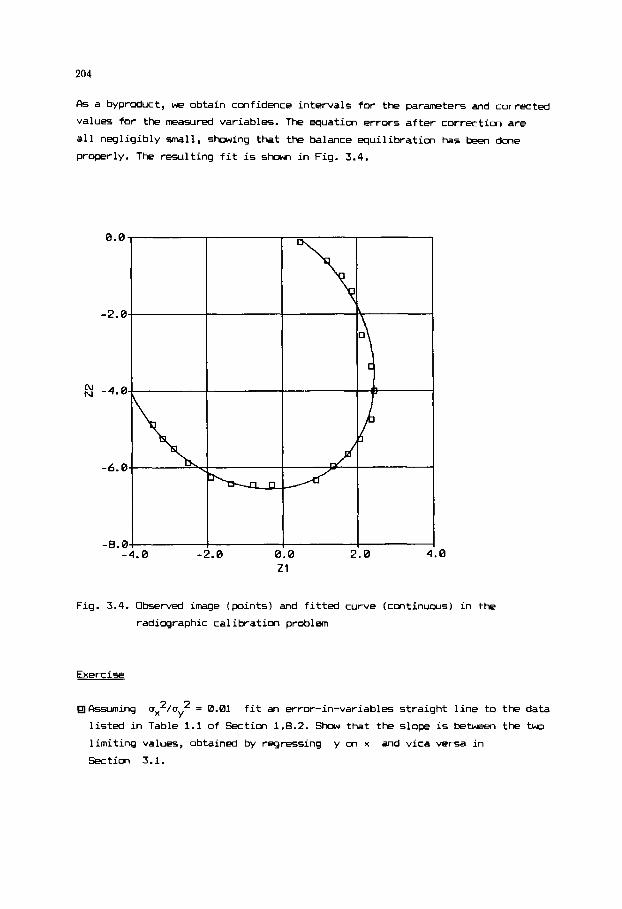
204

As a byproduct, w e obtain confidence intervals for the parameters and corrected

values for the measured variables. The equation errors after correction are

all negligibly small, showing that the balance equilibration b s beRl done

properly. The resulting fit is shown in Fig. 3.4.

N N

, 0 21

Fig. 3.4. Observed image (points) and fitted curve (continuas) in the

radiographic calibration problem

Exercise

Assuming ~ ~ ~ ~ / c r ~ ~ = 0.01 fit an error-in-variables straight line to the data

listed in Table 1.1 of Section 1.8.2. Show that the slope is between the two

limiting values, obtained by regressing y on x and vica versa in

Section 3.1.

205

3.9 FITTIffi ORTHOGONC\L F'CLYNOMIPLS

Y o u can use multivariable linear regression to fit a polynomial

(3.99) r7 n

LA i=0 y = ) aixi

- to the set { (x,, y,); j = 1,2, ..., np 1 of points. The i-th row of the

observation matrix x in (3.20) is then ( 1, xjr xj2, ..., xj" 1. E V ~ for a

polynomial of moderately high degree, however, the resulting cross-product

matrix

This difficulty can be avoided by estimating the parameters

of the function

XTX has a large condition number, and the problem is ill-conditioned.

so, sl, ..., s,,

(3.100)

where Po, Pl, ..., Pn are polynomials, orthogonal on the given set of grid points. To define this property introduce the notation

According to Forsythe (ref. 3 9 ) , the polynomials Pk and P1 are orthogonal

over the grid points

orthogonality of the polynomials

regression problem associated with the model (3.100) is diagonal and hence very

easy to invert. A further advantage is that increasing the degree of the

polynomial from n to n+l, the previous estimates so, 51, ..., sn remain

unchanged.

(xl, xz, ..., xnp), if < Pk(X),Pl(x) > = 0. a/ the

Pi, the cross product matrix of the linear

A h h

The Forsythe polynomials are defined by the recursive relationships

P-l(x) = 0 , Po(x) = 1 , Pi+l(x) = (x-ai+l)Pi(x) - ~ i P ~ - ~ ( x ) ,

where

The least squares estimate of the parameters so, sl, ..., s,, in (3.100) are

simply obtained by

A -" 5.1 = Wi/0.. 11 , where oi = < Y,Pi(x) > .

Rearranging the polynomial (3.100) to the canonical form (3.95') gives the

estimates for the coefficients a,, al, ..., a,,. The following module based on

206

( re f . 40) f i t s polynomials of degree n = 0, 1, ..., ND to the set of N)

points, where ND < W . I f the x j values are not a l l different or numerical

errors are l ike ly to corrupt the results, the module automatically decreases

the maxirmm degree ND, and sets the status flag ER = 1.

Prosram module M52

5500 REH l l l t l ~ t t l l t t t t t l t t t t l l l l t t t t t t t t t t t t t t l l t t t l t t t ~ t 5502 REB t POLYNOHIAL REGRESSION I 5584 REN t USING FORSYTHE ORTHOGONAL POLYNOtllhLS 1 550t REH t t l t i t t t t t t t l l t t t l t l t t t t t t t t t t t t t t t t t t ( t l t t t l l~ l l t t 5508 RE1 INPUT: 5510 REN NP NUMBER OF SAMPLE POINTS 5512 REH X(NP) VALUES OF INDEPENDENT VARIABLE 5514 REH YINP) OBSERVATIONS OF DEPENDENT VARIABLE 5516 RE1 ND 5518 REH OUTPUT: 5520 REN ER ERROR FLAG 5522 RE!! 0 SUCCESSFUL REGRESSION 5524 REH I SPECIFIED ND IS TOO LARGE 5526 REU ( IN THIS CASE A FURTHER OUTPUT IS 5528 REH ND ACTUAL BAXlHUiI DEGREE 1 5530 REH C(J , I J I-TH COEFFICIENT IN THE J-TH ORDER POLYNOMIAL 5532 REH ( V = SUM [C(J,l)IX"II I=0...J ) 5534 REH CINP,J) RESIDUAL SUB OF SQUARES FOR THE J-TH POLYNOHIAL 5536 REN REHARK: HINIHUH SIZE OF (IRRAY C IS NPtNP 5538 REU ---------- GENERATE VALUES OF FORSYTHE POLYNOHIALS 5548 FOR I = i TO NP :ClCl,I)=l :NEXT I :C[l,B)=NP :BE38 5542 FOR J=l TO ND 5549 E R 4 :IF ND)NP-1 THEN ER.1 :ND=NP-I 5546 5548 AL=AL/C(J,B) :ClNP,J)=AL 5550 FOR 1=1 TO tip 5552 5554 5556 NEXT I 5558 SH.0 :FOR 1.1 TO NP :Sil=SH+ClJ,IJtC(J,I! :NEWT I 5568 C(J+l,B)=SH :BE=SH/C(J,B) 5562 5564 NEXT J 5566 RE1 ---------- WEIGHTING COEFFICIENTS OF POLYNOHIALS 5568 '3.0 :FOR 1=1 TO NP :Sl=SH+Y(I) :NEXT I

HAXlHUl DEGREE OF THE POLYNOIIAL I ND(NP )

6 1 4 :FUR I=1 TO HP :AL=ALtYII!1CIJ-l,I)lC(J-I,I) :NEXT I

C( J, I ) = ( I ( I )-AL) tCi J-1, I ) IF 3 E O B THEN CIJ, I )=C(J, I )-BELC(J-Z, I )

IF Sll!=.B@BBlltC(J,0) THEN ER.1 :ND=J-l :6OTO 5566

5570 C(0,0)=l I 5572 FOR 1.1 TO NP-1 :Ci0,1)=8 :NEXT I 5574 C(I,NP)=SII!NP : B E 4 5576 FOR J.1 TO ND 5578 SM.8 :FOR 1:l TO NP :SH=SH+Y(IJtC(J,I1 :NEXT I 5588 AL=CINP, J ) :BU=C( Jtl , a! /C !J ,01 5582 C[JI8)=-ALtC(J-I,8) :IF B E 0 0 THEN C l J , a ) ~ C I J , 0 I - R E l C I J - 2 , 8 ) 5584 FOR I=1 TO ND 5586 C(J,I)~C(J-i,I-l!-ALtC(~-l,I) 5588 IF BEOI THE# CIJ,I)=C(J,I)-BEtC(J-?,!) 5590 NEWT I 5592 FOR I=J+i TO NP-1 :CIJ,I)=0 :NEXT I 5594 C[ J ,NP)=SN/C(Jtl,0 ) : BE-RU 5596 MEXT J

207

5598 REB ---------- CANONICAL POLYNOHIALS AND SUH OF SQUARES 5608 CIO,B)=CI0,NP) tC(0,O) :C(0,NP)=0 : SH.0 : Y=CI0,0) 5602 FOR 1.1 TO NP :SH~SMtlYII)-Y)t(V[l)-Vl :NEXT I :C(NP,B)=SR 5604 FOR J=l TO ND 5606 SR=CIJ,NP) 5608 FOR I:0 TO J :CIJ,I):SHtC(J,I)tClJ-l,I) :NEXT I :CIJ,NP)=0 5618 SH.0 5612 FOR 1.1 TO NP 5614 5616 5618 NEXT I 5620 Cl RP, J )=St4 :b22 I F SMi=ClNP,J-l) THEN ND=J-1:GOTO 5626 5624 NEXT J 5b2b RETURN 5628 RE8 t t t t t t t t t t t t t t t t t t t t t t t t t t t ! & t l ~ t ~ t t t t t t t t l t t t l t t t l

Y=CIJ,J) :FOR K=J-1 TO 0 STEP -1 :Y=YtXlI)+CIJ,K) :NEXT K SH=SH+lVl 1 ) - Y ) 11 'il I)-Y)

Example 3.9 Polynomial regression through Forsythe orthoga-ialization

The LMTA statements of the following program include 12 data pairs

(xi, yi) , where x i s the temperature (K) and y i s the equilibrium vapor

pressure (bar, 1 bar = lo5 Pa) of l iquid oxygen (ref. 41).

We attempt to f i t least squares polynomials of degree 0 through 11 ,

?,

describing the vapor prssure as a functim of temperature.

180 RE\ ________________________________________---------- 102 REH EX. 3.9 . POLYNURIAL REGRESSION 104 RE4 USING FORSYTHE ORTHOGONAL POLYNOHIALS I06 9EM MERGE F55 :08 EEM ---------- D4TA 110 REN 1)lUHBER OF POINTS AND HAXIHUH DEGREE) 112 DRTA i2,ll i14 REM (XlI)-terPp Y(I)-press) i i b Daia 54.35, 8.081580 I18 PRTA 60, 0.807317 128 DATR 70, 0.06235 122 DdTA 80, 0.3083 124 DRTA 90, 0.9943 126 DATA 100, 2.546 128 DATA 110, 5.443 138 DATA 120, 10.21 132 DATA 138, 17.44 134 DATA 140, 27.82 136 DATA 150, 42.23 138 DATA 154.77, 50.87 208 RER ---------- READ DATA AND CALL HODULE 202 READ NP,ND 204 DIH XI NP) ,Y INP ) ,C( NP,NF)

ZPB GOSUB 5500 206 FOR 1.1 TO NP :READ w(ri,v(i) : E X T r

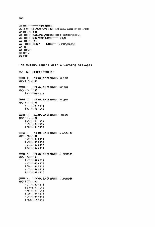
208

PRINT RESULTS 210 REH --_____--- 212 IF ER THEN LPRINT 'ER.1 : R A X , BDnlSSIBLE DEGREE 1S";ND :LPAINT 214 FOR J:t TO ND 216 LPRINT 'DE6REE:';J ,'RESIDUAL SUH DF SQUARES:';C(NP,J) 218 LPRINT USING ' Y ( X ) = L##@##**AA'; C ( J , B ) 228 FOR I=I TO J 222 LPRINT USING " #.##$$#A*A* t XW';C(J,I),I 224 NEXT I 226 LPRINT 228 NEXT J 238 STOP

The outpu t begins w i t h a warning message:

ER.1 : MAX. ADMISSIBLE DEGREE IS 7

DEGREE: B Y ( X )= B.13168Et82

RESIDUAL SUR OF SQUARES: 3512.318

DEGREE: 1 RESIDUAL SUN OF SQUARES: 807.5648 Y(XI= -,34171E+02

8.45189EtBB t X A 1

DEGREE: 2 RESIDUAL SUM OF SQUARES: 54.10914 Y (1 I = 0.51196E+B2

-.136llE+t1 t X A 1 B.fl647BE-02 t X * 2

DEGREE: 3 RESIDUAL SUH OF SQUARES: ,5136249 Y (1). -.34631E+82

8.14353Et81 t X* 1 -.19677E-01 t X * 2 0.98283E-04 t X A 3

DEGREE: 4 RESIDUAL SUH OF SOUARES: 6.469585E-83 Y(X)= -.98362E+00

-.32470E-01 t X A 1 0.32085E-82 t X" '2 -.61456E-04 t X * 3 8.36254E-tb t X* 4

DEGREE: 5 Y ( X ) = -,96379E+01

RESIDUAL SUH OF SQUARES: 4.128297E-03

0.43970Et08 t X" 1 -.67383E-02 t X' 2 8.39624E-84 t X * 3 -.13536E-B6 t X A 4 8.95280E-89 t X * 5

DEGREE: 6 RESIDUAL SUM OF SQUARES: 1.1R9194E-04 Y ( X I = 0.33366Et82

-.23770E+BI L X" 1 0.67954E-01 t X* 2 -.98769E-83 I X* 3 0.76843E-05 I X A 4 -.2937flE-87 t X * 5 0.48386E-10 t X " 6

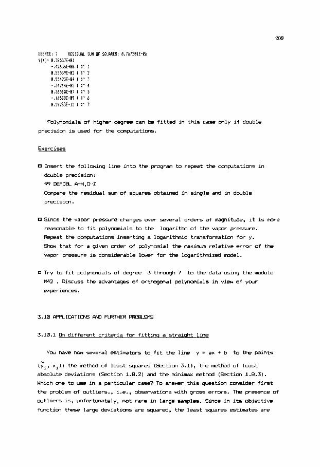
209

DEGREE: 7 RESIDUAL SUH OF SQUARES: 8.767201E-'36 Y ( X i = 8.78537Etll

-.42636Et00 t 1'' 1 0.55539E-82 t X " 2 0.95423E-04 t X " 3 -.34214E-05 t X * 4 0.36510E-07 t X " 5 -,16588E-0? t 1" 6 ~.29za3~-12 t x * 7

Polynomials of higher degree can be fitted in this case only if double

precision is used for the compltations.

Exercises

Insert the following line into the program to repeat the computations in

double precision:

99 DEFDBL &H,C-Z

Compare the residual sum of squares obtained in single and in double

precision.

Since the vapor pressure changes over several orders of magnitude, it is m r e

reascnable to fit polynomials to the

Repeat the computations inserting a logarithmic transformation for y.

Show that for a given order of polynomial the maximum relative error of the

vapor pressure is considerable lower for the logarithized model.

logarithm of the vapor pressure.

0 Try to fit polynomials of degree 3 through 7 to the data using the module

M42 . Dixuss the advantages of orthogonal polynomials in view of your experiences.

3.10 APPLICATIMVS AND FLRll-ER PROaEMs

3.10.1 Q-I different criteria for fittinq a straiaht line

Y o u have now several estimators to fit the line y = ax + b to the points

." (yi, xi): the method of least squares (Section 3.1), the method of least

absolute deviations (Section 1.8.2) and the minimax method (Section 1.8.3).

Which one to use in a particular case? To answer this question consider first

the problem of outliers., i.e., observations with gross errors. The presence of

outliers is, unfortunately, not rare in large samples. Since in its objective

function these large deviations are squared, the least squares estimates are

210

clearly more sensitive to the outliers than the method of least absolute

deviations. The least squares is a m a x i m likelihood estimator so far the

error distribution is normal. In a normal distribution the probability of

wtliers is vanishingly small, and hence their presmce signifies deviation

from the assumed normality. Therefore, if the error distribution is suspected

to be "flat", i.e., the probabilitiy of large errors is higher than expected in

a normal distribution then the more robust least absolute deviations criterion

is preferable.

In practice the error distribution is usually unkncm, and the choice can be

made on the basis of the empirical curtosis of the residuals defined by

2 k = n [Zri4] / [Cri2] , (3.101)

where the

goes from 1 to the number of sample pints. According to (ref. 42), in case

of a large curtosis, k > 3.8 , the sum of absolute deviations is better to use. The other extreme case is indicated by a low curtosis, k < 2.1, w h e n the

error distribution is possibly "sharper" than the normal. In this case the

minimax criterion is a good choice.

ri's are the residuals from a least squares fit, and the sumtion

Exercise

0 Select the suitable criterion for the nicotine - tar data investigated in Sections 1.8.2, 1.8.3 and 3.1. Inspecting the shadow prices in the

minimax estimation omit the mcht suspectible point and repeat the estimations

by the different methods. Discuss the sensitivity of the various estimates

with respect to omitting this pint.

3.10.2 k i q n of experiments for parameter estimation

The best known application of experiment design is to find the extrefrum of a

quantity depending on further variables by observing its value at appropriately

selected points (refs. 43-46). In this section, hawwer, consideration is

restricted to design methods, purported to increase the reliability of

estimates when fitting a model to observations.

A k - point design is described by the design matrix Xk , consisting of k rows. The i-th row of the matrix specify the values o f the the independent

variables to be selected in the i-th experiment. Depending on the linearity or

nonlinearity of the rodel, the design matrix affects the covariance matrix Cp of the estimates according to the expressions (3.301 and (3.45), respectively.

The covariance matrix, in turn, determines the joint confidence region (3.321

211

of the parameters. Our goal is to obtain a confidence region as small as

possible. The size of the ellipsoid (3.32) can be measured in different ways,

and these give rise to various optimality concepts listed in Table 3.7.

Table 3.7 Optimality criteria in experiment design

Optimality concept Cri terion

det[ C 3 ---> min trace[ C 1 --> min P

P

D A E XminC cp 1 --> max

____________________________I_

kcording to Table 3.7, a D - optimal design X minimizes the volume of

the confidence ellipsoid. The mean square length of the axes is minimized in

A - optimal design, whereas

longest axis. In the case of a nonlinear respse functim the Jacobian matrix

(3.411, and hence also the approximate covariance matrix (3.45) depend on the

parameter values, in addition to the design

defined at 5 ~ e fixed parameter vector.

E - optimality means the m i n i m length of the

Xk. Thus optimality of a design is

To obtain a meaningful extremum problem the number of experiments k and

the set of feasible vectors of the independent variables T are fixed. In most

ca5es T

introducing penalty functions

by the methods and modules described in Section 2.4, this direct approach is

usually very inefficient. In fact, experiment design is not easy. The

dimensionality of the extrermm problem is high, the e x t r a are partly m the

boundaries of the feasible region

symnetric in the vectors xl, x2, ..., xk , you have to face the difficult problem of multiple maxima (ref. 44).

is defined by inequalities & 5 xi 5 xu, i = 1,2,.. .,k. Though such constrained extrwm problems can be solved

1, and since the objective functions are

In practice it is more efficient to adopt a less ambitious approach of

"polishing" a starting design xk

objective functim in each iteration and thereby determining a nearly optimal

design. A useful algorithm i5 to drop one point of the current design and add

an optimally selected new point xk to the remaining design Xk-1. This

inner iteration is repeated for each point of the design in turn. Then the

procedure can be restarted updating the first point again. The convergence rate

might be disappointing,

inhermt approximations.

iteratively, increasing the value of the

but high accuracy is not necessary because of the

212

Example 3.10.2 Approximate D - optimal design fo r estimating Michaelis-Menten

parameters

Starting with the substrate values xi = CS i l i n Table 3.4, we construct a

nearly D - optimal design t o estimate the parameters of the response function

(3.55). Since we have 10 measurements i n the s tar t ing design, we f i x k = 10.

The feasible region i s given by xL = 0 and

parameter values, necessary t o be selected a p r io r i , are

and

xu = 5x10-’ mo l / l . The nominal

V = 4X10-’ m o l / ( l a)

K = 4x10-’ ml/l. h s t a n t error variance i s assumed.

In every inner i t e ra t i on step the objective function

Q ( x ) = det{ Jz-lJk-l + j(x;V,K)jT(x;V,K) 1 (3.1022)

i s minimized subject t o the constraint

correspcnding to the r m i n i n g experiment design Xk-l, denoted by JkP1, does

not depend on x , and j i s the column vector of pa r t i a l derivatives a t x . Evaluating (3.102) over a course g r id we can f i nd a t most two local maxima.

xL < x 5 xu, where the Jacobian

Therefore, the program designed t o solve t h i s problem f i r s t divides the

interval CxL,xu], each of the two subintervals bracketing one of the maxima. [h

each interval the single maximum is localized by module M25, and the larger one

i s selected fo r the new point of the design. As shorn i n Table 3.8, the f i r s t

three p i n t s are irmediately replaced by xu. I n the next 5 inner i terat ions,

b v e r , the global maximum i s located a t inner points o f the feasible

interval. Final ly, (3.102) takes i t s maximum value again on the upper end w h e n

replacing the last 2 p i n t s . The design obtained i n the f i rst outer

i terat ion (i.e., a f ter updating a l l the 10 points) remains almost unchanged

subsequently, with the inner points approaching t o a single value. The

resul t ing design decreases the volume of the (approximate) confidence e l l ipso id

of the parameters by a factor of 2 wi th respect t o the s tar t ing design.

Table 3.8 Wte r i terat ions of the experiment design procedure

Design p i n t s xi~103, ml/ l ater QXl@

i terat ion 1 2 3 4 5 b 7 8 9 10

0 1.02 3.02 5.02 8.02 10.02 15.00 20.00 30.00 40.02 50.00 2.S96 1 50.00 50.02 50.02 14.74 14.- 14.63 14.75 15.13 50.00 50.00 4.5854 2 50.02 50.02 50.02 15.42 15.42 15.34 15.33 15.38 50.00 50.00 4.5939

b 50.00 50.02 50.00 15.38 15.39 15.38 15.38 15.38 50.02 50.02 4.5939

213

In this example the approximate design consists only of two differmt points

with replicates. Restricting the number of points to k = 2 right at the beginning, the problem can be solved by hand calculations yielding the same

result. Y o u should not draw, however, overly general cmclusion from this fact,

since the number of different points in a D - optimal design can exceed the number of the parameters. Nevertheless, the optimal design normally involves a

relatively small number of different points, and the corresponding observations

are hardly suitable for validating the model. Thus the methods of this section

apply only when the form of the response function is no more questionable. The

need for replicates is a disadvantage also in kinetic analysis, where in a

single experimntal run the variables can be sampled at points that are not t w

close. Such additional constraints, however, can be incorporated into the

design procedures (see, e . g . , refs. 47-48).

Exercise

0 Repeat the design procedure of Example 3.10.2 assuming constant relative

variances.

3.10.3 Selectins the order in a family of horol~cus models

In Example 3.5.1 we used ridge regression to confirm that the simpler model

(3.33) is preferable to (3.64), though the latter gives slightly better fit.

Such model selection problems are faced in many applications, particularly when

considering a homologous family of candidate models. For example, in polynomial

regression we should select a degree n. A similar problem, discussed in

Chapter 5, is to select the order n of a linear differential equatim when

identifying a pharmacokinetic model.

Example 3.5 has certainly convinced you that the test fitting model is not

necessarily the one to chc-=e. In fact, it may be overparameterized with respect

to the available data, leading to inflated or even meaningless estimates of the

parameters. In addition, a t m complex model usually gives unsatisfactory

predictions, even slightly apart from the observed values of independent

variables. Which model should be then adopted? The simplest rule is that model

cmplexity (i.e., its degree or order) should be increased only while the

residual variance is significantly decreasing. This can be tested cunparing the

residual variances of different models ty the F-criterion. This test is

not "sharp" enwgh and frequently suggests a too complex model. A number of

criteria has been proposed that take the number of parameters into account more

explicitely (for reviews see e . g . , refs. 49-54)). The most poplar one is the

Akaike's Information Criterion (ref. 511, suggesting to choose the model for

214

which the quantity

AIC = - 2 log (maximium likelihmd) + 2 np (3.103)

takes its minim value, where np is the number of the parameters. If the

assumptions (i)-(vi) of the least squares method are valid, minimizing (3.103)

is equivalent to minimizing the simple expression

AIC’ = Q(G;np)/t? + 2 np , (3.104)

where Q(̂ p;np)

weighting coefficients

parameters. In practice 2 is replaced by its estimate s2. At this point it

is advantagas to use a c m s2, not depending on the number of parameters

of the particular model. Obviously, the a priori choice of

affects the atcome of the test.

is the minim value of the weighted wn of squares with

wi = c?/cri2, found for the model containing np

s2 significantly

Exercise

0 Select the degree of the polynomial describing the logarithnic vapor pressure

of oxygen as a function of the temperature (see Example 3.9).

Suppose the vapor pressure is exact to three digits and give an estimate

for the logarithms. Apply (3.104) replacing 2 with 5’.

s2

3.10.4 Error-in-variables estimation of van Laar wrameters from

vapor-liauid eauilibrium data

At low pressures the following equations are valid for a binary vapor-liquid

mixture :

(3.104)

where

mole fraction of component 1 in the liquid phase mole fraction of component 1 in the vapor phase pressure

equilibrium vapor pressure of pure component i activity ccefficient of component i.

x1 Y1 P T temperature pio(T) 7i

The functions pio(T) equation:

are supposed to be know exactly, given by the Fhtoine

log pio(T/K)/Pa = A i - Bi/CT/K + Cil .

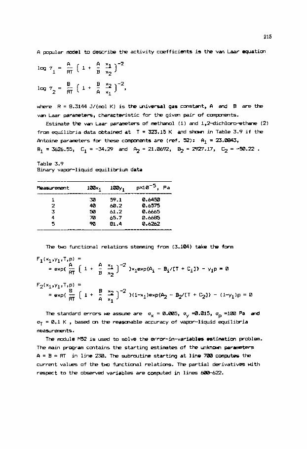
215

A popllar model to describe the activi ty cwf f ic ients i s the van Laar equation

where R = 8.3144 J / ( m l K ) i s the universal gas constant, CI and B are the

van Laar parameters, characteristic for the given pair of compxlents.

Estimate the van Laar parameters of methanol (1) and 1,2-dichloro--ethane (2)

from equil ibria data obtained a t

Antoine parameters for these components are (ref. 52) :

T = 323.15 K and shaw, i n Table 3.9 i f the

A 1 = 23.0843,

B1 = 3626.55, Ci = -34.29 and = 21.0692, % = 2927.17, % = -54).22 *

Table 3.9 Binary vapor-liquid equilibrium data

Measuremeot 1 ~ 1 0 ~ ~ 1ml p ~ 0 - 5 , Pa ----

1 30 59.1 0.6450 2 40 60.2 0.6575 3 50 61.2 0.6665 4 70 65.7 0.6685 5 50 81.4 0.6262

The two functimal relations stemming f rom (3.104) take the form

The standard errors we assume are ux = 0.005, u 4.015, up 400 Pa and Y uT = 0.1 K , based on the reamable accuracy of vapor-liquid equi l ibr ia

measurmts . The module M52 i s used to solve the error-in-variables estimation problem.

The main program contains the starting estimates of the unknow, parameters

A = B = RT

current values of the two functimal relations. The part ial derivatives with

respect to the observed variables are canputed i n l ines 600-622.

i n l ine 230. The subroutine starting a t l ine 700 canputes the

216

108 REn ........................................................... 182 REH EX. 3.18.4 VRN LRRR PRRRNETERS (ERROR-IN-VARIRBLES HETHOD) 104 R E I MERGE Hl6,HlR,H4l,H45,H52 186 RE1 ---------- DATA 188 REH ( NH ) 110 DRTR 5 112 REH ( X1 Y1 P/PA T/K 1 114 DRTR 8.38, 8,591, .6458E5, 323.15 116 DATA 8.48, 8.602, .6575E5, 323.15 118 DATA 8.58, 8.612, ,6665E5, 323,15 128 DATA 8.70, 0.657, .6685E5, 323.15 122 DRTR 8.98, 8.814, .62b?E5, 323.15

282 READ NH 284 NZ.4 :NK=2 :NP=2 :IH=28 3 6 DIH T(NH,?tNZ 1 ,V(NH,NKl ,R(NZ ,P(NP) I Z (NZ 1, X ( 2tNZ) ,Y INK) ,FINK) 208 DIH E(NK,NZ ) ,R(NP,NP), C(NP,NP) ,U( NP,NP) ,B(NP) ,DlNP) ,S(NP) 218 DIH G(NK,NP),OINK,NKI 212 FOR 1.1 TO NH 214 FOR J=l TO NZ :READ TI1,Jl :NEXT J 216 NEXT I 21B BN1=23.4883 :BN1=3626.55 :CN1=-34.29 :REI ANTOINE PIRAHETERS 220 RN24'1.0692 :BN212927.17 :CN2=-56.22 :REH

READ DATA 288 REM _______--_

' 222 RU=8.3144 :REH 6RS CONSTANT 224 R l I )=( .885) "2 :R(2 )= ( . 815)T :R(3 )= ( 188)*2 : R ( 4 ) = ( . 1 )^2 :REH VARIANCES 226 REfl ___--___-- ITERGTION CONTROL PRRBHETERS AND INITIRL GUESS 228 EP=.BBI :EZ=.B81 :IH=28 230 PI 1 ]=RUt323.15 :P(2)=RUt323.15 232 GOSUB 5288 234 IF EROB THEN LPRINT 'STATUS FLA6:';ER 236 STOP 688 REM ________-_ JACOBIAN HRTRlX OF F WITH RESPECT TO I 682 RR=P(l) :BB=P(Zl :PT=Z131 :T=2(4) 684 XI=Z(l) :X2=l-X1 :YI=Z(2) :Y2=1-Y1 686 Pl=EXPlRNl-BNI/ ( TtCNlI ) :PZ;EXP(RN2-BN2/ (TtCN2) ) 618 Sl=RA/RU/T/(ltAA/BBtXl/X2)*2 610 S2=BU/RU/T/lltBB/AAtX2/X1)*2 612 SI=EXP(SI) :62=EXP(S2) 614 E(1,l): 6ltP1-2t6ltXltPltBR/RU/TtRR/~B/XZ*2/(liXl/X2tRA/~U]A3 616 E(l,Z)=-PT :E(1,3)=-Yl :E~1,9)~-XltPlt61tSI/T~61t~ltPl~BNl/(T~CNl~A2 618 E(2,1):-62tP2~2t62tX2tP2t~B/RU/TtBB/AA/Xl~2/(ltX2/XltBE/RR]*3 b28 E 12,2 )= PT : E (2,314 2 :E (2,4 1 =-XZtP2t62tS2/Tt62tX2&P2tENZ/ ( TtCN2) *? 622 RETURN

FUNCTION EVALUATION 718 RE! _ _ _ _ _ _ _ _ _ _ 782 AR=P(l) :BB=Pl2) :PT=2(3) : T - Z ( 4 ) 784 Xl=Z(lI :XZ=l-XI :Y1=2(2) :YZ=I-Yl 7616 PI=EXP(AHl-BNI/ (TtCN111 :PZ=EXP(RN2-BN2/ (TtCN2) ) 708 SI=AA/RU/T/ (ltAA/BBtXI/X2)*2 712) SZ=BB/RU/T/ (ItBB/AAtX2/X1)^2 712 61=EXP(SI) :62=EXP(S2) 714 F(1)=6ltXltPl-YltPT 716 F(2)=62tX2tP2-YZtPT 718 RETURN

982 6OSUB 5398 984 RETURN

DBLIGATORY STITEMENT 9Bfl REH ---___-_--

After two cuter iterations the following results are obtained.

217

...................................................................... PARPHETER ESTllPTE ST. ERROR LOWER BOUND UPPER BOUND

P ( 1 ) 8.51359Et04 8.19477Et83 0.48939EtB4 9.53779Et94 PI 2 ) 8.43207Et04 6.52429Et02 0.41996Et94 0.44418E+04

......................................................................

HEAS I Z( I ) H E M 2 I I ) CORR EOURTION ERROR AFTER CORRECTION

1 9.30000Et9B 2 0.59109Et00 3 8.64508Et05 4 0.32315EtB3

1 B.400BBEt0B 2 0.6020BEtEB 3 0.6575BEtB5 4 0.32315Et03

I 0.50E90Et00 2 0.6128BEtB0 3 0.66658Et05 4 0.32315EtU3

1 0.7BBB0EtEE 2 0.6579@Et00

4 0.32315Et03

1 0.90000Et00 2 0.8140BEtEB 3 B.62620EtB5

3 0.66850E+B5

4 8.32315Et93

0.29879Et09 B.59596EtB0 0.64525Et15 0.32309EtB3

0.39967Et90 0.61214Et09 0.65761Et95 0.32312EtE3

0.5BB18Et90 8.62400EtUB B. 666lEEtB5 8.32324EtB3

0.69947Et0B 0.66676Et00 8.66835Et05 6.32319Et83

9.98060EtBB 0.8104BEtBB E.62621Et85 0.3231 5Et03

F( 1 )=-.915625 F( 2 )=-9.765625E-03

F ( 1 )=-.046875 F ( 2 )=-2.734375E-02

F I 1 )=-3.90625E-83 F( 2 )=-3.9Bb25E-83

The van Laar parameters CI = 5135.9 J/ml and B = 4320.7 J/ml yield a

good fit. The observed variables are only slightly corrected to satisfy the

d e l equations. The quantity "equation error after correction" is expressed in

Pascals, hence the above values are negligible mall .

You can meet almost all the difficulties of parameter estimation w h e n

evaluating vapor-liquid equilibria data (implicit functional relations among

several variables, corrupted by measurement errors that are likely to be

correlated (see, e . g . , ref. 53).

W S

1 M.G. Kendall and CI. Stuart, The Advanced Theory of Statistics. vol. 2,

2 N.R. Draper and H. Smith, CIpplied Regression Chalysis. 2nd ed., John Wiley, Inference and Relationship, 3rd ed., Griffith, London, 1973.

1981.

218

3 R.R. Hocking, Developments in linear regression methodology: 1959-1982,

4 Y. Bard, Nonlinear Parameter Estimation. Academic Press, NEW York, 1974. 5 D.M. Himlblau, Process Analysis by Statistical Methods, John Wiley,

New York, 1970. 6 F.S. wmd, The use of individual effects and residuals in fitting equations

to data. Teclnometrics, 15 (1973) 667-696. 7 J.Durbin and G.S. Wattscn, Testing for serial correlations in least squares

regression, I . , Biometrika, 37 (1958) 409-426. 8 K. Schwetlick, Kinetixhe Methoden zur Chtersucl-ung von Reaktionmechanim.

MB Deutxher Verlag der Wissenxhaften, Berlin, 1974. 9 J.N. Brmsted and W.F.K. Wynne-Jones, Trans. Faraday SOC. 25 (1929) 59. 10 Y, Bard, Comparison of gradient methods for the solution of nonlinear

parameter estimation problems, SIAM J. W r . Anal. 7 (1970) 157-186. 11 D.M. Himlblau, Applied Nonlinear Programming, McGraw-Hill, New York, 1972. 12 J. Garcia-Peh, S.P. Azen and R.N. Bergman, On a modification of

Marquardt's cunprmise: Rationale and applications. Appl. Math. Complting,

Technometrics, 25 (1183) 219-23.

12 (198 1-17. 13 L. Nazareth, Some recmt approaches to solving large residual nonlinear

14 K. Levenberg, A method for the solution of certain nonlinear problems in

15 D.W. Marquardt, Pn algorithm for least squares estimation of non-linear

16 R.A. Alberty and F. Daniels, Physical Chemistry, 5th ed., John Wiley,

17 G.F. F r m t and K.B. Bixhoff, Chemical Reactor Analysis and Design,

18 W.B.S. Newling and C.N. Hinshelwood, The kinetics of the acid and alkaline

19 M.J.C. Crabbe, An enzyme kinetics program for desk-top computers,

20 D. Garfinkel and K.A. Fegley, Fitting physiological models to data,

21 D.M. Bates and D.C. Watts, Relative curvature measures of nonlinearity,

22 D.A. Ratkowsky, Nonlinear Regression Modeling, Marcel Dekker, New Yorrk

23 A.E. Hoerl and R.W. Kennard, Ridge regression: Biased estimation for

24 R.I. Jennrich and P.F. Sam-, Application of stepwise regression to

25 S.Vajda, P. Valkb and T. Turthyi, Principal component analysis of kinetic

26 S. Vajda and T. Turthyi, Principal canponmt analysis for reducing the

least squares problems. SIAM Rev., 22 ( 1 W ) 1-11.

least squares, hart. Appl. Math., 2 (1944) 164-168.

parameters. SIAM J. Appl. Math., 11 (1963) 431-441.

New York,lW.

Joln Wiley, New York, 1979.

hydrolysis of esters, J. Chem. Sa, 23 (1936) 1357-1364.

Cmplt. Biol. Ned. 4 (1982) 263-283.

Am. J. Physiol. 246 (19B4) R641-R650.

J. R. Statist. Soc., Ser. B 42 (1980) 1-25.

1983.

nonorthogonal problw, Teclnometrics, 12 (1970) 55-67.

nonlinear estimation. Techncwtrics, 10 (1968) 63-72.

models, Int. J. Chem. Kinet. 17 (1985) 55-81.

Edelsonfield-Noyes model of Belousov-Zhabtinsky reaction, J. Phys. C h . W (1986) 1664.

from several responses. Biometrika, 52 (1965) 355-365.

rmltiresponse modelling, Technometrics, 21 (1979) 291-298.

Some problw associated with the analysis of multirespmse data, Technometrics, 15 (1973) 33-51.

response parameter estimation, SIAM J. Sci. and Stat. Comp., 8 (1987) 49-55.

61 (1965) 8-13.

27 G.E.P. Box and N.R. Draper, The Bayesian estimation of c m parameters

26 D.D. McLean, D.J. Pritchard, D.W. Bacon and J. h i e , Singularities in

29 G.P.E. Box, W.G. Hulter, J.F. MacGregor and J . Erjavec,

30 D.M Bates and D.G. Watts, A generalized Gauss-Newton procedure for rmlti-

31 D.L. Ripps, Adjustment of experimental data. Chem. Engng. Prq. Symp. Ser.

219

32 G.A. Almky and T. Sztanb, Checking and correction of measurements on the

33 W.D. Deming, Statistical Wjustment of Data, John Wiley, New York, 1943. 34 H.I. Britt and R.H. Luecke, The estimation of parameters in nonlinear

implicit models. Technanetrics, 15 (1973) 233-241. 35 P.M. Reilly and H. PatintrLeal, A Bayesian study of the error-in-variables

model. Technmtrics, 23 (1981) 221-227. 36 H. Patino-Leal and P.M. Reilly, Statistical estimation of parameters in

vapor-liquid equilibrium. AICK J. 28 (1982) 580-587. 37 P. Valkb and S . Vajda, &I extended Marquardt-type procedure for fitting

error-in-variables models. Comput. C h . Engng. 11 (1987) 37-43. 38 J.H. Wilkinson and C. Reinxh, Handbook for Outmatic Computation, Vol. 11.

Linear Algebra, Springer Verlag, New York, 1971. 39 G.E. Forsythe, Generation and use of orthogonal polynomials for data-fitting

with a digital computer. J. SIM, 5 (1957) 74-88. 40 D.B. Marsland, Data fitting by orthogonal polynomials, in. CAM

Thermodynamics (ed. R.V. Jelinekl, Sterling Swift, Manchaca TX, 1971. 41 N.B. Vargaftik,

Nauka, Moscow, 1972 (in Russian) 42 J.E. Gentile, W.J. Kennedy and V.A. Spmsito, 0-1 least absolute values

estimation, h. Statistics, M, (1977) 838-845. 43 J.C. Kiefer, Design of experiments, in. Collected Papers 111, Springer,

NEW York, 1985. 44 V.V. Nalimv and N.A. Chernova, Statistical methods of design of extremal

experiments, Nauka, Moxow, 1965 (in Russian) 45 G.K. Krug, Yu.6. Sosulin and V.A. Fatuw, Design of experiments in

identification and extrapolation, Nauka, Moxow, 1977. 46 B. Kanyb, Parameter sensitivity analysis for designing of experiments

in kinetics, Fkta Biochim. Biophys. &ad. Sci. h g . 12 (1978) 24-28. 47 D.Z. D’Argenio, Optimal sampling times for pharmacokinetic experiments,

J. Pharmacokinet. Biopharm. 9 (1981) 739-755. 48 J.J DiStefano 111, Optimized blwd sampling protocols and sequential design

of kinetic experiments, Am. J. Physiol. 240 (1981) R259-FQ65. 49 I.J. Lecntaritis and S.A. Billings, Model selection and validation methods

for nm-linear systems, Int. J. Cmtr. 45 (1987) 511-341. 50 E.M. Landau and J.J. DiStefano 111, t”Lltiexpmentia1, multicompartmental and

noncompartmental modeling 11, Data analysis and statistical considerations, h. J. Physiol. 246 (1984) R665-R677.

51 H. Akaike, A new look at statistical model identification, IEEE Trans. Aut. Control, AC-19 (1974) 716-723.

52 R.C. Reid, J.M. Prausnitz and T.K. Sherwood, The Properties of Gases and Liquids, 3rd ed. PkGraw-Hill, NEW York, 1977.

53 S. Kemhy, J. Manczinger, S. Skold-Jorgmsen and K. Tbth, Reduction of thermodynamic data by means of the multirespmse maximum likelihood principle, AICE J. 28 (1982) 21-3.

basis of linear system models. Probl. Control. Inf. Theory, 4 (1975) 59-69.

Handbook of Thermphysical Data of Gases and Liquids,

220

Chapter 4

SIGNAL PROCESSING

Many experimwlts result in a sequence { (xi,yi), i = 1, 2, ..., m 3 of

data pairs. As in the previous chapter, w e assume that there exists a

functional relationship y = f(x) between the two variables, and hmce refer

to (xl, ..., x,) and (yl, ..., y m ) as grid points and function values,

respectively. The form of this function is, lmwever, often unknowr. In other

cases it may be deduced from physical principles, but is too complex far

meaningful parameter estimation, with m a n y parameters of no particular

interest. In both situations we wish to predict s ~ e properties of f directly

from the observations

as follows:

(xiryi). The most important quantities to estimate are

i) the functim value f(x) between two grid points (interpolation);

ii) the derivative f'(x) (numerical differentiation); and

iii) the integral f(x)dx , where the limits a and b satisfy the b

a

inequalities x1 5 a < b 2 xm (numerical integration).

The important application of numerical differentiation is locating the

extrema or inflection points of the curve. Finding the area under the curve

involves numerical integration.

Since f(x) is known only at the grid points, to solve these problems we

must connect the data by saw plausible interpolating function. Its form s b l d

be sufficiently general so as to be able to approximate large classes of

functions, but simple enough to deal with. By far the most c m a m 9 such

functions are polynomials. If we use all data pairs simultaneously, the

interpolation is called global. In many cases, hDwever, local interpolation is

a better choice, considering only n < m grid points a r m d the point x of

interest. Local linear and quadratic interpolation (i.e., n = 2 and n = 3 , respectively) are the most familiar procedures. W h e n the interpolating function

has been selected, numerical differentiation and integration are

straightforward. For example, with local linear interpolation shown in

Fig. 4.1, the estimate of the derivative is (yi+l-yi)/(xi+l-xi) at all

x - 1 - < x 5 xi+l , whereas J:f+lf(x)dx 2 (yi+l + yi)/(xi + 1-xi)/2 by the well 1

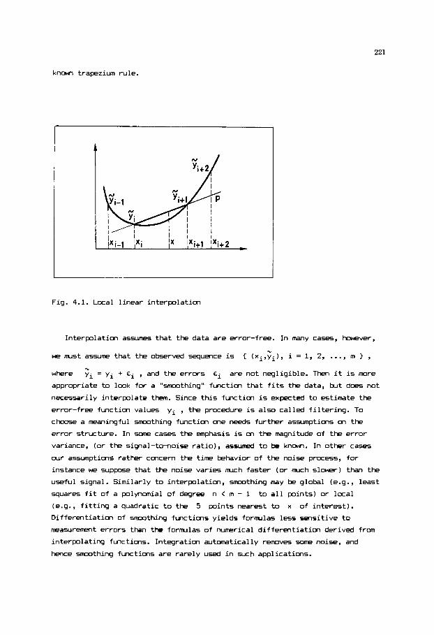
221

know, trapezium rule.

c c

I Fig. 4.1. Local linear interpolation

Interpolation as- that the data are error-free. In many cases, however,

w e must assume that the observed sequence is c i = I, 2, ..., m I , where Li appropriate to look for a "-thing" function that fits the data, but does not

necessarily interpolate them. Since this function is expected to estimate the

error-free function values yi , the procedure is also called filtering. To

choose a meaningful -thing function one needs further assumptions on the

error structure. In some cases the emphasis is on the magnitude of the error

variance, (or the signal-to-noise ratio), aswned to be k n m . In other cases

our assumptions rather concern the time behavior of the noise process, for

instance we suppose that the noise varies much faster (or rmch slower) than the

useful signal. Similarly to interpolation, -thing may be global ( e . g . , least

squares fit of a polynomial of degree n < m - I to all points) or local

(e.g., fitting a quadratic to the 5 points nearest to x of interest).

Differentiation of smwthing functions yields forrmlas less sensitive to

measurement errors than the forrmlas of numerical differentiation derived from

interpolating functions. Integration automatically removes 5ome noise, and

hence -thing functions are rarely used in such applications.

n,

yi = yi + Gi , and the errors are not negligible. Then it is more

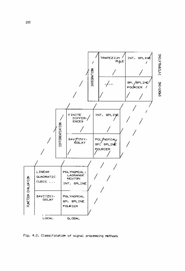
222

TRAPEZIUM R U k E

/

/

5 r( i +

9 I N T . SPLIN c( +

a

i? / E? CI

/

2 S'PpLINE/ FOURIER / I

/

L I NEAR

QUADRAT I C

C U B I C . . .

SAV I TZKY- GOLAY

/

/

F I N I T E D I FFER-/ ENCES

OLAY y-

/

POLYNOMIAL: LAGRANGE NEWTON

I N T . S P L I N E

POLYNOMIAL

SM. S P L I N E

FOUR I ER

LOCAL GLOBAL

Fig . 4.2. Classificatim of s i g n a l process ing methada

223

Each signal processing method dixussed here involves sane function which is

either interpolating or smoothing, and is either local or global approximation

of the data. This results in the two-way classification of the methods show, in

Figure 4.2, where the quadrants of each card list methods of the same family

for the particular application.

Signal processing may also involve parameter estimation methods (e.g.,

resolution of a spectral curve into the sum of Gaussian functions). Even in

such cases, however, we may need non-parametric methods to approximate the

position, height and half-width of the peaks, used as initial estimates in the

parameter estimation procedure.

In this chapter we restrict consideration to nm-recursive signal

processing. A good introduction into recursive filtering can be found in the

b w k of Bozic (ref. 1). Another interesting field not discussed here is to

modify conventional analytical methods to produce signals, w h o s e direct huMn

interpretation is no longer necessary and possible ( e . g . , correlation

chromatography). The interested reader may consult the review paper (ref. 2).

As shown in Fig. 4.2, we have several methods to solve any particular

problem. The choice primarly depends on the sample size, and hence we introduce

the following classificatim:

i) small samples (5-15 points);

ii) medium samples (lE-llZEi pints); and

iii) large samples (from 50 points).

Small samples are practically error-free in most cases ( e . g . , data in

thermodynamical tables), but given over an irregular mesh. Ch the other hand,

large samples almost invariably represent the "raw" output of a measuring

device, or are obtained by sampling a continuous signal. In this class the grid

pints are equidistant that may simplify data processing. In medium

samples we often have sme assumption on the signal-to-noise ratio while in

large samples the spectral properties of the noise process are m r e or less

known.

There is an extensive mathematical literature devoted to interpolation,

function approximation, numerical differentiation and integration (refs. 3-5),

but many methods are not particularly useful for signal processing. For

example, there is a large variety of efficient methods of integrating

numerically a function that can be cmplted at any desired point. In signal

processing, however, the data are a priori given, and the class of applicable

methods is considerably restricted. In addition, many classical formulas are

very simple so that discussing them we include only three modules.

More attention will be given to two families of very general methods. The

224

first is based on the use of spline functions, and is going to replace many

classical procedures for interpolation, smwthing, numerical differentiation

and integration. The second family contains the Fourier transform spectral

methods, and it has such an extensive list of potential applications that we

can discuss only of the most basic mes.

4.1 CLASSIW MTHODS

4.1.1 Interpolation

In global polynomial interpolation we fit the polynomial

P,l(X) = a,lxm-l + a,p m-2 + ... + do

to the points

equations

pW1(xi) = yi, i = 1, 2, ..., m .

{ (xi,yi), i = 1, 2, ..., m } by solving the set of . .

If the grid points are distinct, the solution of (4.2) is

unique. The correspcnding polynomial can be given in several explicit forms

different from the canonical form (4.1). For instance, it can be complted as a

linear combination

a,, al, ... am-l

of the Lagrange base polynomials defined by

TI (x-xi)

TI (xj-xi) - i#j

i #j

Lj(X) =

(4.3)

(4.4)

The classical Lagrange forrmla is not efficimt numerically. One can derive

m r e efficient, but otherwise naturally equivalent interpolation forrmlas by

introducing finite differences. The first order divided differences are

defined by

f(x.) - f(x-

xi - xi-1 f ( Xi, xi-l ) = ---L--2d

where f(xi) = yi. Similarly

defined recursively by

, i=2, ... m, (4.5)

the (k+l)-th order divided differences are

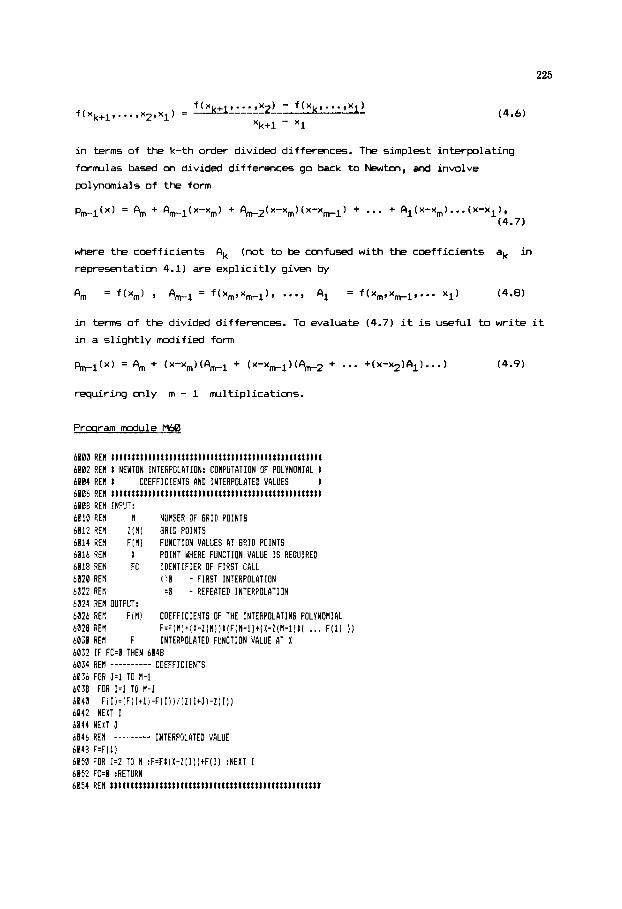
i n terms of the k-th order divided differences. The

225

(4.6)

simplest interpolating

formulas based on divided differences go back t o h t o n , and involve

polynomials of the form

+ A,2(x-xm) + ... + ~l(X-Xm)...(X-X1)' (4.7)

where the coefficients Ak (not t o be confused with the coeff ic ients ak i n

representation 4.1) are e x p l i c i t l y given by

Am = f ( x m ) , Aml = f ( X m , X m - l ) , ..., A 1 = f(Xrn,Xm-1,"' Xi) (4.8)

i n terms of the divided differences. To evaluate (4.7) i t i s useful t o wr i te i t

i n a s l i gh t l y modified form

requiring only m - 1 rmlt ip l icat icns.

Prmram m u l e PA0

6000 RE! t I t t t tttttt t t t t t t It ttttttt I t t I I I It t t t t t t t t t t t t t t t t t 6002 REIl t NEWTON IMTERPOLPTION: COWPUTATION OF POLYNONIAL t 6004 REH I COEFFICIENTS AND INTERPOLATED VALUES t 60B6 RE! t I t ttttttl I t t I t It tttt tttt It t t ttt t tttt tttttttt It t t t t OBBB REN !N?CT: 601B RE5 tl NJNFER OF 6RID POINTS 6012 RE8 Z(1) GRID POINTS A014 REM F[N) FUNCTION VALUES A! 6RID POINTS 6016 REF X POINT WHERE FUNCTION VALUE IS REQUIRED 6018 RER FC IDENTIFIER OF FIRST CALL 6820 REM (':I - FIRST INTERPOLATION be22 RE8 10 - REPEATED INTERPOLATION 6024 RE! 0UTPL;T: 6026 REK Fin) COEFFICIENTS OF THE INTERPOLATING POLYNOMRL 6028 REH F:FlM)+IX-ZlH) ! t [F[N-11+!X-Z!R-l) t ( , . . F(1) ) 1 6050 RE! F INTERPOLATED FUNCTIDN VALUE AT X 6032 IF FC=0 THEN 6048 0034 RE!! ---------- COEFFICIENTS A076 FCR J.1 TO H-1 6038 FOR 1.1 TO N-J 6040 6042 NEXT I

Fl I ) = l F i I+l!-F( I ) ) i (Zl I+J)-Z( I) 1

5a44 NEXT J INTERPOLATED VALUE b045 REH ._________

6848 F=F[I) 6050 FOR !=2 TO M :F=FtlX-ZII))tFlI) :NEXT I 6852 FC.0 :RETURN 6054 REN t t t t t t I I tttt ttt t It t t It tlttt t t t t t t It tttttttttttttttt

226

There are two operations performed in the module. First, it determines the

coefficients Ak

at the specified X . Both operations are performed if the first call flag FC

has a nonzero value on the inplt.

of the function values, and the module sets the value FC = 0 . In a second (and in any subsequent) call with the same data but with a different

coefficients are not recomputed.

in the expression (4.7). Second, it calculates the polynomial

The coefficients will be stored in the place

X the

Example 4.1.1 Determination of enthalpy by Newton interpolation

Each DATFI line of the following main program gives a temperature T and a

corresponding molar enthalpy value

(ref. 6). The units are K and kJ/ml, respectively. We find the molar

enthalpy at the temperature

# ( T I - p ( 0 ) of SiF4 in gaseous state

T = 298.15 K.

188 RE1 ........................................................... 102 REH EX. 4.1.1 NEWTON INTERPOLATION 104 REH NERGE N60 L86 REH ---------- DATA 10B REH (NUNBER OF POINTS) IIU DATA 9 112 RER (1,K H-H0,kJ/nolI

116 DATA 388, 15.492 118 DATA 408, 23.367 128 DATA 588, 32.826 122 DATA 608, 41.225

126 DATB 800, b0.637

138 DATA 1000, 88.836 280 REH ---------- READ DATA

204 D M Zln),F(H) 206 FOR 1=1 TO Il 288 READ Z(I),F(I) 218 NEXT I 212 RE1 ---------- CALL INTERPOLATION MODULE 214 FC.1 :X=298.15 216 LPRINT 'NEUTON INTERPOLATION, NUHBER OF PO1NTS:";H 218 GOSUB 6000 220 VI=STR196)05, '-I I 222 LPRINT V1 224 LPRINT USING ' T = I t # . t # K 226 LPRINT V$

114 DATA 290, e.722

124 DATA 708, 50.799

128 DATA PBB, 70.666

202 READ n

H( T )-H( 8 )-I$ .##I kJ/nol" ; X ,F

228 STOP

The outpit of the program is as follows.

227

NEYTON INTERPOLBTION, MUilEER OF POINTS: 9 ............................................. T=298.15 K H I 1) -H(0)=15.356 kJ/&ol ---_____________________________________-----

Global polynomial interpolation is restricted to ~jmall samples of fairly

gmd data. If there are many grid points, the resulting higher order polynomial

tends to oscillate wildly bet- the tabulated values as show in Fig. 4.3.

I I I I i b

Xi-1 xi xitl X i t 2

Fig. 4.3. Fh interpolating polynomial p oscillating a r m d the "true"

functim f .

This oxillation may have nb relation at all to the behavior of the "true"

function. Therefore, we cannot recarmend global interpolation except for

m a l l samples. In large samples interpolation is rarely needed. For medium size

samples low order local interpolation considering 3 - 6 nearest neighbors of the point

is lmal cubic interpolation in the Aitken form programmed in the

following module.

x of interest does the job in most cases. The m t popular m e t W

228

Proqram module M b l

6100 REII t l t t t l t t t ~ t t t t ~ t t t t ~ 1 l l t l 1 l ~ l t 1 l 1 1 1 l ~ ! t 1 ~ l l l t l 1 l l 1 t 6102 REfl 1 LOCAL CtiBIC INTERPOLATION 1 6104 REH t l t l t t t t t t t1 l t t t l t t t~ t t t l11 l~ t l~ t l t l l t l t l l t l l t l t11 l 6106 REF INPIT: 6108 RE1 N NUBREF! OF GRID POINTS

6112 REH F(R) FUNCTION VALUES AT 6RID POINTS t114 RE! X GIVEN POINT bllb REfl WTPJT: 6llE REr F INTERPOLATED FUNCTION VALUE 6li0 FOR 11.4 TO H-1 6122 IF Z(6-l)bX THEN 6128 6124 NEWT K 6 1 3 K=n 6128 F3.F [i -3) : F?=F IR-2) :Fl=F (K-1) :F=F[ C ) 6130 Dj=Z(K-Z)-X :DZ=Z(K-ZI-X :Dl=Z[K-l)-X :D=Z(K)-W 6132 F?=(F3tDWZtD3)/ (D2-D3) 6134 Fl.IF3tDl-FlrD3;/[Dl-D3) 6136 F ZIF3tD -F tDSi/(D -D3)

6lSh) F =!F21C -F tDZ)/(D -D2! b142 F =1FltD -F tDI)/[D 4 1 ) b144 RETURN 6140 R E 1 ~t l t t t l t t t t l l t t t t t1 t t t t t t1 t t11 l t t t~ l t t l~ l t t t l1 t l l1 t

tiia REH z(n) WID POINTS

613 Fl=(F?lDl-FltD2)i(Dl-D?)

The module selects the four nearest neighbors of X and evaluates the cubic

interpolating polynomial.

Evaluation of a function outside the range of the grid points is called

extrapolation. While extraplation is based on the same ideas as interpolation,

it is mch more hazardous and shwld be avoided whenever possible.

4.1.2 Smmthinq

Smoothing of noisy data is justified if the sampling frequency is

sufficiently high, and hence the sample contains information for adjusting the

observed function values by kind of averaging. Then the smmthing function

enables us to evaluate function values at both the grid points and bet- them

a5 well. Global least squares polynomial fit is the most traditional method of

smoothing for small and medium samples. Orthogonal polynomials and the program

module M55 are useful to carry cut such calculations.

For large samples global polynomial smoothing is either not sufficiently

flexible (if the selected degree is low) or faces the same problems as in the

case of interpolation (if the selected degree is high). Local smathing

usually gives better results. This involves least squares fit of polynomials of

degree n < Zk to the 2k + 1 points (X-k,Y-k), ... (Xo,yo), ... (XkrYk),

229

-h3 h2 -h 1

h3 h2 h 1

. ah3 4hZ 2h 1 ,

0 0 0 1

where 2k is sufficiently smaller than m and xo is a selected grid point

of interest. The fit is particularly simple if the grid points are equidistant

and the aim is to obtain a corrected value xo. Then this estimate can

be computed as the linear combination yo at

r , Y =

(4.10)

of the considered 2k + 1 function values. The coefficients ci and the

denaninator F of the forrmlas (4.10) have been compiled by Savitzky and Golay

(refs. 7-6) for several values of k and n.

Table 4.1 shows the Savitzky - Golay coefficients obtained by fitting a

quadratic or cubic (these two yield identical coefficients for ) to 5, 7, 9

and 11 points. The way to select the number of points is discussed in (ref. 9).

The use of t m many points is hazardous, since increasing the “extent of

smoothing” such fits can distort also the useful signals. Therefore, the m x t

popllar forrmla involves only 5 points and the cubic

R(X) = a3x3 + a2x2 + alx + do . (4.11)

Derivation of the coefficients in (4.10) for this case is very simple. If h

is the distance bet- the grid points denoted by

(O,yO), (h,;l) and (2h,q2), then the observatim matrix X and observation

(-2h,;-2), (-h,;-l), I

vector 3 introduced in Section 3.2 are given by

c

Y-2

Y-1

YO

r

I

c

Y1

;2

(4.12)

Ejy (3.23) the least squares estimates of the coefficients in (4.11) are

(4.13)

230

Since

formula we were lmking for.

p3(0) = a. , the first expression of (4.13) is the Savitzky - Golay

Table 4.1 Coefficients for local quadratic or cubic smmthing by Savitzky and Golay

5 -3 12 17 12 -3 35 7 -2 3 6 7 6 3 - 2 21 9 -21 14 39 54 59 54 39 14 -21 231 11 -36 9 44 69 84 89 84 69 44 9 -36 429

In addition to their simplicity the Savitzky - Golay formulas are well

suited to real time filtering. While more advanced methods such as -thing by

spline functions or by Fourier techniques as- the knowledge of the entire

sample, to apply (4.10) we have to wait mly for further k points. If k is

Once fixed the extent of smoothing can be increased by applying the procedure

several times. If the sampling frequency is high, it may be sufficient to pick

up each (Zk+l)-th point and wrooth only these ones using their nearest

neighbors.

4.1.3 Differentiation

The derivatives of the unknown functim are estimated by the derivatives of

an interpolating or smoothing function fitted to the given set of data. Global

interpolating polynomials wildly oscillating bet- grid points are not

suitable for estimating the derivatives. Fk show, in Fig. 4.3, we may expect

particularly bad estimates at the grid points where the polynomial crosses the

"true" curve.

The familiar forrmlas of numerical differentiation are the derivatives of

local interpolating polynaials. A11 such formulas give bad estimates if there

are errors in the data. To illustrate this point consider the case of linear

interpolation where the divided difference (yi+l - - xi) estimates

the derivative at xi < x < xi+l . Let = c? denote the variance of

the measurwnent errors. We are usually m r e concerned with the relative errors

a/yi, the inverse of the signal-to-noise ratio. If the errors are independent,

then

r r

r

D2{;i+l - ;i) = 2 2 and hence the relative error in the slope is given

231

error of the slope may be much larger than the relative error in the data.

Notice that this error is additional to the one introduced w h e n approximating

the function by a straight line.

It follows that the formlas of nwrical differentiation do not apply to

noisy sequence of data. Formulas based on the differentiation of local

smoothing polynomials perform somewhat better. These are also of the form

(4.10) if the derivatives are required only at the grid points. For example,

the derivative of (4.11) is

~ ' ~ ( 0 ) = al , where al is given by (4.13) as a linear combination of the function values. The coefficients of the formulas of -thing differentidtion

based on the fit of a cubic (ref. 7) are show, in Table 4.2. To obtain correct

numerical values you should multiply the denaninator by the distance h as

shown in (4.13).

P'~(x) = 3a3x2 + 2a2x + al . Therefore,

Table 4.2 Coefficients for local cubic smoothing differentiation by Savitzky and Golay

2k + 1 x-5 X-4 X-3 x-2 x-1 xo xi x2 x3 x4 x5

5 1 -8 0 8 -1 12 7 22 -67 -58 0 58 67 -22 252 9 86 -142 -193 -126 0 126 193 142 -86 1188 11 302-294 -532-503-296 0 296 323 532 294 -302 5148

Although numerical differentiation is considered as a routine step in signal

processing, our discussion tries to emphasize that its results heavily depend

on the choice of the interpolating or -thing function. Different methods may

lead to much deviating estimates. Nevertheless, from frequently sampled data

we may be able to locate e x t r a or inflection points by nwrical

differentiation, since zero-crossing of the first or second derivatives is

Mmewhat more reliable than their values.

The next d u l e is based on the five point Savitzky - Golay formulas listed

in Tables 4.1 and 4.2. It returns both the smoothed function values and the

estimates of the derivative. The formulas are extended also to the four

outermost points of the sample, where (4.10) does not directly apply.

232

Prwram module M2

mu REH t t t t t t t t t t t t t t t t t t t t t : t t t t t t t t t t t t t i ~ ; ; t : : r t : t t ~ i ~ t 6202 RE# t 5-POINT CUBIC SMOOTHING BY SAVITZCY AND GOLAY t 6204 RER t t t t t ~ ~ ~ t t t t t t t t t t t t l t t f t t ~ ~ 1 : t ~ t ~ t t t t l t t t t t t t t t t t t 6286 PEfl IMFUT: b208 REY N #UMBER OF GRID POINTS 6210 RER FIN1 FUNCTION VALUES AT 6RID POINTS b212 2EM OUTPUT: 5214 RE! SI1,N) S l B , I ) SHOOTHED FUNCTION VALUES 6216 PEW b218 RER REMARK: 6 2 8 S10,1~=i267tF111~12LF12]-1BtF~3!~12tF141-~tF(5))1210 6222 S l B , 2 ~ ~ 1 2 1 F l l l ~ 2 7 t F ~ 2 ) t 1 2 t F ~ 3 ] - B t F [ 4 ) t 2 t F [ S ) ) / 3 5 6 2 3 FOR 1 4 TO N-2 b226 SI0,I 1=1-3tFI 1 - 2 ) t l Z t F l 1-1 l t l 7 t F I I )+12tF[ I t 1 ) -3 tF [ I t ? ) 1/35 6228 NEXT I 6230 SiU,Nl~i287tFlNl~12tFl~-l~-lBtF~N-?)~l2tF~N-3l-3tF~N-4ll/2l0 6232 6234 5 I1 , 1 I =i -125tF I 1) t 1 3 6 t F 121t4RtF13) -8BtFl 4) t 2 9 t F I51 1 /84 6236 S(1,21=1 - S 7 t F ( l ) -~~Fl2)~3~tF~3!*39tF~4)-lS~F(5))/l~b 6239 FOR 1-3 TO N-2 1248 S l l , I ) = I F 1 I -Z) -RtF( 1-1 I t B t F I It1 )-F( I t 2 1 1/12 b242 NEXT I 6144 Sl 1 N l = 1125 tFlN)-l36tF(N-ll-4BtFlN-2l~~BtF lN-31-29tF "-4) 1 /a4 6246 6248 RETURN 6250 RE! t t t t t t t l t t t l t t t l t t t 1 t t t t : t t t ~ t t t t t t t t t t t t t t f t t ~ ~ t t l

S ( 1 , I ) SMOOTHED FIRST DERI'VATIVES END POINTS ARE ALSO PROCESSED

SI0 ,N- l I= lZ tF IN1 t 2 7 t F I N - 1 I t l 2 t F "-21 -8 IF lN-3 l t2 tF(N-4 ] 1135

S l 1 ,N-1 ) = I 97 IF IN) +3 tF(N- l I -36tF(N-2)-3TtF(N-3) t15tF(N-4 1 i /1?6

Note that the the g r i d poin ts are n o t s p e c i f i e d on the i n p t . The d e r i v a t i v e

is numerically correct i f the d i s t a n c e h between the g r i d p o i n t s is 1.

Otherwise, to obta in t h e d e r i v a t i v e a t the I-th point you rmst d i v i d e S ( 1 , I )

by t h e d is tance .

Example 4.1.3 Detection of end p o i n t s i n potent icmetr ic t i t r a t i o n by the method

of Savitzky and Golay

In potent icmetr ic titratim a vol tage is obtained f r m an e l e c t r o d e that is

s e n s i t i v e to an imic species =uch a5 , i.e., the pH of the s o l u t i o n i n

t h i s case. We w i l l consider t h e t i t r a t i o n of t h e mixture of a s t r o n g a c i d ( K 1 )

and a weak ac id (M$UFl) with NaOH ( r e f . 10). ck 2 m l vol- of the base

are given t o the a c i d i c s o l u t i o n , t h e pH increases and w h e n one of the a c i d s

is neut ra l ized t h e pH changes very rap id ly by a small a d d i t i m of NaM . We

want to f i n d these maximum poin ts of the f i r s t d e r i v a t i v e of the t i t r a t i o n

curve. In t h e following main program the DFITA l i n e s conta in 32 d a t a pairs,

each cons is t ing of the volume of t h e added NaM i n m l and the measured pH.

F i r s t we call the module to obta in the f i r s t der iva t ive . Then t h i s

d e r i v a t i v e is placed i n t o t h e a r r a y F , and by repeatedly c a l l i n g the module

w e obta in the estimate of the second der iva t ive .

233

109 REH ________________________________________------------------- 102 REH EX. 4.1.3 SMOOTHED DERIVATIVES BY SAVITZKY RND 60LAY 104 REH MERGE Hb2 106 REM ---------- DATA 108 REH (NUNBER OF POINTS) 118 DATA 32 112 REH (V,m1; pH) 114 DATA 2.4, 2.642, 2.6, 2.706, 2.8, 2.786, 3.1, 2.877 116 DATA 3.2, 2.986, 3.4, 3.126, 3.6, 3.295, 3.8, 3.480 118 DATA 4.8, 3.659, 4.2, 3.816, 4.4, 3.952, 4.6, 4.874 128 DATA 4,8, 4.183, 5.8, 4.285, 5.2, 4.384, 5.4, 4.488 122 DATA 5.6, 4.579, 5.8, 4.682, 6.8, 4.791, 6.2, 4.988 124 DATA 6.4, 5.845, 6.6, 5.211, 6.8, 5.444, 7.1, 5.859 126 DATA 7.2, 8.617, 7.4, 9.747, 7.6,18.134, 7.8,18.348 128 DATA 8.8,18.491 , R.2,18.684, 8.4,10.692, 8.6,18.7b6 200 REN ---------- READ DATA 282 READ N 284 Dln I IN) ,F (N) , S l 1 ,N) ,A1 ( N ) ,AZ(N) ,A3(N) ,A4 IN) 286 FOR 1.1 TO N 288 READ Z(II,F(I) :!Al(I)=F(Il 218 NEXT I 212 RE! ---------- SMOOTH TWICE 214 DI=Z(2)-2(1) 21b GOSUB 6208 218 FOR 1.1 TO N :A2(1)=S(B,I) :A3(1)=S(l,I)/DI :F(I)=R3(1) :NEXT I 220 GOSUB 6288 222 FOR 1.1 TO N :A4(1)=S(l,I)/D2 :NEXT I 224 REn 226 REH ---------- PRINT RESULTS 228 V$=STRlN6~145,"-*) :LPRINT V$ 230 LPRINT 'V,nl pH smoothed pH first second" 232 LPRINT " derivative ' 234 LPRINT V1 236 V1$= * 1.11 81.111 11.111 111.111 111.111 238 FOR 1.1 TO N 240 LPRINT USING V11;7(I) ,Al(I) ,RZ(I),A3( I) ,A4111 242 NEXT I 244 LPRINT V$ 246 STOP

The program gives the output a5 f o l l m .

............................................. V,rl pH smoothed pH first second

derivative

2.48 2.642 2.642 8.292 8.425 2.68 2.706 2.707 8.357 8.299 2.88 2.786 2.785 8.427 8.313 3.88 2.877 2.876 0.492 6.462 3.28 2.986 2.987 8.618 8.768 3.48 3.126 3.127 8.779 8.758 3.68 3.295 3.296 8.900 8.395 3.88 3.488 3.479 8.926 -0.157 4.08 3.659 3.658 0.846 -0.548 4.28 Z.816 3.815 0.729 -0.536 4.40 3.952 3.953 8.642 -8.381

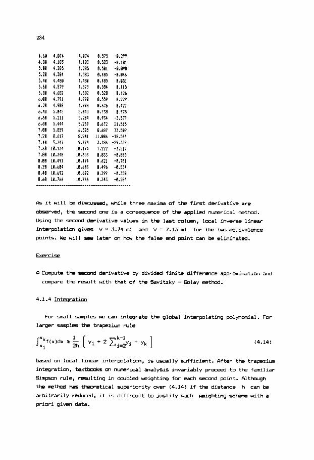
234

4.60 4.174 4.88 4.183 5.88 4.285 5.20 4.384 5.40 4.480 5.61 4.579 5.88 4.682 6.80 4.791 6.28 4.988 6.40 5.045 6.68 5.211 5.88 5.444 7.08 5.859 7.20 8,617 7.48 9.747 7.68 10.134 7.81 18.348 8.88 11.491 8.20 10.604 8.48 11.692 8.60 18.766

4.074 4.183 4,285 4 * 383 4.480 4.579 4,682 4,798 4.908 5.043 5.214 5.269 6.385 8.201 9.774

10.174 10.353 10.494 18.683 18.692 18.766

1.575 -8.299 8.523 -8.181 8,501 -8.090 8.485 -0.846 0.485 8.051 8.584 0.115 0.528 8.126 8.559 8.229 0.626 8.427 8.738 0.978 8.934 -3.579 1.672 21.565 8.687 33.589

11.806 -18.564 3.186 -29.339 1.222 -3.517 8.833 -8.865 0.621 -8.781 0.496 -0.534

8.343 -0.284 8.399 -8.358

ck it will be discussed, while three maxim of the first derivative are

observed, the secmd one is a consequence of the applied numerical method.

Using the second derivative valu- in the last co1um-1, local inverse linear

interpolation gives V = 3.74 ml and V = 7.13 ml for the two equivalence

points. We will see later on how the false end point can be eliminated.

Exercise

0 Cunplte the second derivative by divided finite difference approximation and

cunpare the result with that of the Savitzky - Golay method.

4.1.4 Inteqration

For small samples we can integrate the global interpolating polynomial. For

larger samples the trapezium rule

(4.14)

based on local linear interpolation, is usually sufficient. FIfter the trapezium

integration, textbwks m numerical analysis invariably proceed to the familiar

Simpxn rule, resulting in doubled weighting for each secmd point. Althargh

the method has theoretical superiority over (4.14) if the distance h can be

arbitrarily reduced, it is difficult to justify such weighting schffne with a

priori given data.

235

Exercise

Discuss the behavior of the Simpson formla on a "measured" data sequence

similar to 1,-1,1,-1, ...

Show that integration amplifies the signal-tcmoise ratio if the errors are

independent .

4.2 SPLIN FUUCTIONS IN SIawL PRDCESSING

Local cubic interpolation results in a function whose derivative is not

necessarily continuous at the grid points. With a nm-local adjustment of the

coefficients we can, hDwever, achieve global differentiability up to the second

derivatives. Euch functions, still being cubic polynomials between each pair of

grid points, are called cubic splines and offer a "stiffer" interpolation than

the strictly local approach.

4.2.1 Interpolatinq splines

We find the cubic spline interpolating the points C (xi,yi), i = 1, 2, ..., n 1. Let pi(d) denote the cubic polynomial over the interval [xi,xi+ll

of length hi = xi+l - xi , where d = x - xi. To define the n-1 cubics we

need 4(n-1) coefficients. The available constraints are as follows:

(a) The cubics are interpolating ones, and hence

pi(0) = yi , i=1,2, ... n-1; pi(hi) = yi+l , i=1,2, ... n-1.

(b) The continuity of the first derivative implies

= p'i(0), i=2,3, ... n-1,

(4.15)

(4.16)

(4.17)

(c) whereas from the continuity of the second derivative we have

p"i-l(hi-l) = ~"~(01, i=2,3 ,... n-1. (4.18)

Thus we have 4n-6 equations, and need two further constraints to define the

coefficients uniquely. In m t case5 these are chosen according to me of the

following alternatives.

236

i) Assume that the second derivative vanishes at the end points x1 and xn,

resulting in the equations ~"~(0) = 0 and ~"~-l(h,-l) = 0 . The derived function is called natural spline.

ii) The first derivative has arbitrarily fixed values at the end points,

P'l(0) = Y ' O and P'n-l(%-l) = Y ' ~ .

It can be verified that the set of linear equations given by the constraints

has a unique solution both for cases i) and ii), if the grid points

xl, x2, ..., xn are distinct (ref. 11).

quantity

To illustrate a special smoothness property of natural splines, define the

Obviously, S = 0 for a straight line. If S is small for a

function, it indicates that f does not wildly oscillate over

[xl,xn] o f interest. It can be shown that m g all functions

given

the interval

that are twice

continuously differentiable and interpolate the given points, S takes its

minimum value on the natural cubic interpolating spline (ref. 12).

It remains to calculate the coefficients that define the interpolating

spline. [he can obviously solve the 4(n-1) constraint equations directly, but

there exists a much m r e efficient algorithm. Let mi and mi+l denote the

second derivatives of the cubic pi at d = 0 and d = hi, respectively. The

derivative is a linear function, given by

Integrating the function (4.20) twice and determining the two integration

constants from the constraints (4.15) and (4.16), the cubic polynomial

obtained in the form

pi is

i = 1,2, ... n-1 . (4.21)

Now we differentiate (4.21) once and exploit the constraints (4.17). The

resulting equations are

231

i = 2, 3, ..., n-1 . (4.22)

If we select the end conditions

m l = O and m,,=0. (4.23)

i), the further equations are

Wopting assumption ii) instead, equations (4.23) are replaced by

2hlml + hl- = - Y * ~ ] and hl

(4.24)

In both cases the resulting system of equatims is tridiagonal and can be

easily solved by the special method presented in Sectim 1.5. (hce the

values are knorn, equations (4.21) can be easily rearranged to obtain the

polynomial coefficients. Camputing the function value and the derivatives at

any point x is then straightforward, whereas integration is facilitated by

the relationship

mi

valid for any cubic.

Prwram module M63

6385 REH INPUT: 6388 REH N

6312 REH F ( N ) 6314 REIl EC 6316 R E 1 6318 REfl 6320 RER 5322 REH D1 6324 REH DN 6526 REH OUTPUT: 6328 RE1 S14.N) 6338 RER

6316 REH Z(NI NUHBER OF GRID POINTS 6RID POINTS (KNOTS) FUMCTION VALUES I D E N T I F I E R FOR SELECTING END CONDITIONS

NOT 0 - FIRST DERIVATIVES GIVEN AT END POINTS

F I R S T DERIVATIVE AT X=I(l) F I R S T DERIVATIVE AT X=Z(N)

0 - NATURAL SPLINE

T H I S CASE REQUIRES FURTHER INPUTS:

S ( J , I I COEFFICIENTS OF THE J-TH DEGREE TERHS ( 5 4 . . . 3 ) S(4,I) INTEGRAL VALUE FRON Z(l) TO Z(I)

238

6332 FOR l = I TO N-1 6334 S ~ U , I ~ ~ Z ~ l ~ l l - Z ~ l l : 5 ~ l , ~ ) ~ ( F ( ~ t l ~ - F ( ~ ) ) / 5 ( 0 1 ~ ) 6336 NEXT I 6338 S($,N)=B 6340 5(3,1)=2tS(0,1) 6342 I F ECOU THEN 5(2,1)=3t~S(l,lI-D1)

6346 S=S(B, 1-1 1 /S(3,1-1) 6344 FOR 1.2 To N

b358 S~3,I~=2:(S~0,I~tS~0,I-lll-sts~u~1-1~ 6348 IF EC.0 AND 1.2 THEN S=0

6352 IF I (N THEN 5~2,11~~~~S~1,1)-5(1,1-11~-5~5(2,~-1) b354 NEXT I 6356 I F ECOB THEN S~2,N~~3t~DN-S(1,N-l))-StS~Z,N-l) 6358 I F EC.0 THEN 512,N)=8 6360 S(Z,N)=S( 2, N ) IS( 3,N) :S( 3,N)=U 6362 FOR 1.N-1 TO 1 STEP -1 6364 S(?,1)~(S(2,I]-S(B,l)tS(?,Itl))/S[~,I) 6366 IF E C 4 AND 1=1 THEN S(2,1)=8 6368 S11,1)~S~1,3)-S(B,I)t(21S(2,I)~S(2,I~l))13 6378 5(3 I I I W 2 , It1 )-5(2 I 1 ) IS(0, I ) 13 6372 NEXT I 6374 S( I ,N)=S( 1 ,N-1 )tS(B,N-ll t (S (2,N-1 )tS(?,N) ) 6376 S(4,1)=8 6378 FOR 1.2 TO N 6388 SzS( 4,I-1 l*S(B, 1-1 t I F ( I ltF( 1-1 ) ) 12 b382 5 ( 4 , I +S( B, 1-1 )^3t ( S( 2 , I 1 tS ( 2 , 1-1 ) 1 112 6384 S( B, I-1) =F( 1-11 6386 NEXT I 6388 S( B,N) =F( N ) 6398 RETURN 6391 REA t t t t t l t t t t t t t t t l t t t t t : : t : : : : : : : : : : : : t t t t~~:: : : : : t : :

With the end condition flag EC = 0 m the input, the module determines the

natural cubic spline function interpolating the function values stored in

vector F. Otherwise, D1 and DN are additional input parameters specifying

the first derivatives at the first and last points, respectively. Results are

returned in the array S such that S(J,I), J = 0, 1, 2, 3 contain the 4

coefficients of the cubic defined on the I-th segment bet- Z(1) and

Z(I+l). Note that the i-th cubic is given in a coordinate systm centered

at Z ( 1 ) . The module also calculates the area under the curve from the first

point Z(1) to each grid point Z(1) , and returns it in S(4,I) . The entries in the array S can be directly used in applications, but we provide a further

module to facilitate this step.

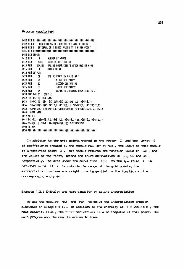
239

Proaram module M64

6488 REH I & t I I t t t t t t t t t l t t t t t t t t ~ l t t t t I t I I t l t ~ t l t t t t l ~ t t t ! ~ t 6482 REH t FUNCTION VALUE, DERIVATIVES AND D E F I N I T E t 6404 REH I t 6406 REH t t l t I t t t t t t t t t t t t I t t ~ ~ t t l t & t & & k I I t t t t t t ~ ~ t t t t t t t t ~ t 6488 REH INPUT: 6410 R E 1 N NUNBER OF KNOTS 6412 REH Z(N) GRID POINTS (KNOTS) 6414 REH S(4,N) SPLINE COEFFICIENTS (FROH H63 OR 165) 6416 REH X GIVEN POINT 6418 REH OUTPUT: 6428 REH SB SPLINE FUNCTION VALUE AT X 6422 REH 51 F I R S T DERIVATIVE 6424 REH 52 SECOND DERIVATIVE 6426 REH 53 THIRD DERIVATIVE 6428 REH 54 D E F I N I T E INTEGRAL FROH Zll) TD X 6438 FOR I=N TO 1 STEP -1 6432 IF XU(I1 THEN 6442 6434 6436 6438 6440 60TO 6448 6442 NEXT I 6444 S=X-ZII) :S0=[5[2,1)tS+S(1,1) )tS+SIB,l) :S1=2tSIZ11 )tS+S(l,!) 6446 S2=512,1) :S34 :S4=StISB+S(B,l) )/2-StStSIS2/6 6448 RETURN 6458 REIl t t I t t t t t t t t t t t l t t I I I I I t t l & t t t t l l t t t t I t t t t l t t t t t ~ t t &

INTEGRAL OF A CUBIC SPLINE RT A 6IVEN.POINT

S=X-Z[I) :58=( ( S( 3, I )tS+S(2, I ) )tStS(l,I) )tS+S(0,1) S1=(315(3, I)tS+2tS(2, I))tS+S(l, I) :S2=6tS(3, I)tS+2tS[2, I) 53=6tS( 3, I ) :S4=S( 4, I ) +St (SBtS(B, I ) )/Z-StStSt lS2+S(2, I ) ) 112

In addition to the grid points stored in the vector 2 and the array S

of coefficients created by the mdule M63 (or by M69), the input to this module

is a specified point

the values of the first, secmd and third derivatives in S1, 52 and S3 , respectively. The area under the curve from Z(1) to the specified X is

returned in 54. If X is outside the range of the grid points, the

extrapolation involves a straight line tangential to the function at the

corresponding end point.

X . This module returns the functicn value in S0 , and

ExamDle 4.2.1 Enthalpy and heat capacity by spline interpolation

We use the mdulg. MaJ and M64 to solve the interpolation problem

discussed in Example 4.1.1. In addition to the enthalpy at T = 298.15 K , the heat capacity (i.e., the first derivative) is also cmputed at this point. The

main program an0 the results are as follows.

240

180 REN ____-___________________________________------------------- 182 REfl EX. 4.2.1 SPLINE INTERPOLATION 184 REM HERGE H63, H64 186 REH ---------- DATA 188 REH (NUHBER OF POINTS) 118 DATA q 112 REM (T,K H-Hfl,kJ/~l) 114 DATA 280, e.722 116 DATA 388, 15.492 118 DATR 488, 23.367 128 DATA 580, 32.826 122 DATA baa, 41.225 124 DATA 788, 58.799 126 DATR EBB, 68.637 128 DATA 988, 78.666 130 DATA 1881, 88.836

202 RERD N 284 DIH Z(N),F(N),S[4,N) 286 FOR I=1 TD N 288 READ Z(l),F(l) 210 NEXT I 212 LPRINT "NATURAL CUBIC SPLINE INTERPOLATION" 214 RE^ _ _ _ _ _ _ _ _ _ _ CALL SPLINE DETERHINATION AND EVRLUATIDN HODULES 216 EL=% :GOSUB 6380 218 X=298.15 :6OSUB 6488 228 VI=STRING$( 45, '-' 1 222 LPRINT V1 224 LPRINT USING "T=W.$# K 226 LPRINT USING ' C p 4 .### J / (001 K)';SIk1008 228 LPRINT VS 238 STOP

READ DATA 288 REfl _-_--_--__

H(T)-H(81=$#.### kJ/nol';X,SB

NATURAL CUBIC SPLINE INTERPOLATION

4.2.2 Smoothins solines

c I f the data C (x i ,y i ) , i = 1, 2, ..., n > are noisy, i t i s not reasonable

to force a function f to pa55 through the measured values. Suppose we have an

estimate di of the standard error of the i-th function value. ThRl a

suitable measure of the distance of any smoothing function

measurement points i s the sum of squares

f f rom the

(4.26)

If the squared distance F2 i s greater than the number of points n, then the

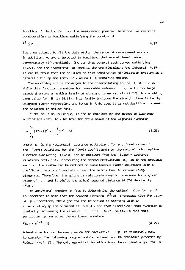
241

function f is too far from the measurement points. Therefore, we restrict

consideration to functions satisfying the constraint

F2(n, (4.27)

i.e., we attempt to fit the data within the range of measurement errors.

In addition, we are interested in functions that are at least twice

continuously differentiable. a7e can draw several such curves satisfying

(4.27), and the "smoothest" of them is the one minimizing the integral (4.19).

It can be shown that the solution of this constrained minimization problem is a

natural cubic spline (ref. 12). We call it wnwthing spline.

The smoothing spline converges to the interpolating spline if di -> 0.

with too large While this function is unique for reasanable values of

standard errors an entire family of straight lines satisfy (4.27) t b s yielding

zero value for S in (4.19). This family includes the straight line fitted by

weighted linear regression, and hence in this case it is not justified to seek

the solution in spline form.

di,

If the solution is unique, it can be obtained by the method of Lagrange

multipliers (ref. 13). We look for the minimum of the Lagrange function

L = 'n 1

[f'8(x)12dx + -(F2 - n) P

X1

(4.28)

where p is the reciprocal Lagrange multiplier. For any fixed value of p

the 4(n-1) equations for the 4(n-1) coefficients of the natural cubic spline

function minimizing (4.28) can be obtained from the Euler - Lagrange

relations (ref. 13). Introducing the second derivatives mi as in the previous

section, the system can be reduced to simultanwus linear equations with a

coefficient matrix of band structure. The matrix has 5 nonvanishing

diagonals. Therefore, the spline is relatively easy to determine for a given

value of p , and it yields the actual squared distance (4.26) denoted by F2(p).

The additional problem we face i5 determining the optimal value for p. It

is important to note that the squared distance

of p . Therefore, the algorithm can be viewed as starting with an

interpolating spline obtained at

gradually increasing the value of p until (4.27) holds. To find this

particular p we solve the nonlinear equation

Fz(p) increases with the value

p = 0 , and then "streching" this function by

A Newton method can be used, since the derivative F'(p) is relatively easy

to compute. The following program d u l e is based on the procedure proposed by

Reinxh (ref. 13). The only essential deviation from the original algorithm is

242

i n the formula for the correction 4 :

where the additional square root convergence promtion factor can sanewhat

improve the convergence a t the beginning of the iteration where

satisfies the inequality

~ ' ( p )

0 < ~ ' ( p ) << n .

Prosram module M65

6588 REll t t t t t t t t I t t t tt tt t ttt t tttt tt tt t t t t t t t tI t tt t t t t t ttkt t 6582 REH t DETERHINBTION OF SHOOTHIN6 CUBIC SPLINE t 6584 RER I HETHOD OF C. H. REINSCH t 6506 RER t t t tl t t t t t t t I t t t t t tt tt t t t t I t t t t t t t t ttt t t tttl t k t tt t t 6508 REH INPUT: 6518 REH N NUHBER OF 6RID POINTS 6512 REH Z ( N ) 6RID POINTS (KNOTS) 6514 REll F(N) FUNCTION VALUES 6516 REH D(N) STANDARD ERRORS AT 6RID POINTS

6528 RER OUTPUT: 6522 REH ER STATUS FLAG 6524 REH 8 SUCCESSFUL COHPLETITION 6526 REH 1 SOLUTION IS P STRAIGHT LINE 6528 REH 2 NURBER OF ITERATIONS IS INSUFFICIENT 6538 REH 6532 RER 6534 REH AUXILIARY ARRAY: 6536 RER R(6,N) 6 5 3 R(5,8)=8 :R(5,1)=8 :P=B 6548 R('d,B)=8 :R(B,l)=B :R(B,N)=B :RG?,N)=B 6542 H=Z(Z)-Z(I) :F=(F(2)-F(l))/H 6544 FOR 1.2 TO N-1 6546 6.H :H=Z(I+l)-Z[I) 6548 E=F :F~(F(I+l!-F(I))/H 6550 S(B,I)=F-E :R(3,1)=2t(6tH)/3 :R(9,1)=H/3 t 5 5 2 R(2,1)=D(I-1!/6 :R(B,I)=D(ltl)/H 6554 6556 NEXT I 6558 FOR 1:2 TO N-1 6568 S I 1 , I )=R(B, I ) tRI 0, I )MI1 , I ) tR( 1 I I )tRl2,I) tR (2,l) 6562 S(2,1)=R(B,1~tR~1,lt1~~R11,1~tR12,1~1) 6564 6566 NEXT I

6518 REH In HAXIHUH NUHBER OF ITERATIONS

S(4,N) S(J,I) COEFFICIENTS OF THE J-TH DEGREE TERHS (5.8 ... 3) S(4,I) INTEGRhL VALUES FROH I l l ) TD Z(I)

R(1,I )=-D( I )/ED( I) /H

IF I(N-1 THEN S13,1)=R(0,I)tR12,It2) ELSE S(3,1)4

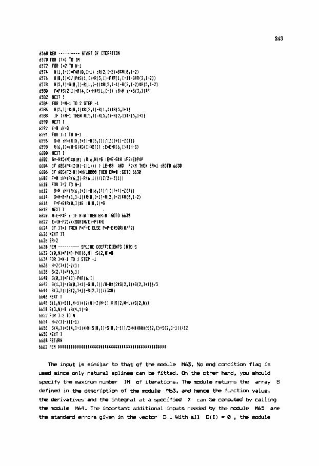
243

6568 REfl ---------- START OF ITERBTION

6572 FOR Iz2 TO N-1 6574 RIl,I-l~=FlRl8,I-l~ :RI2,1-21=6tR(8,1-2) 6576 6578 6588 6582 NEXT I 6584 FOR 1.N-1 TO 2 STEP -1 6586 R(5,1)=R(B,I)tR(5,1)~[l,l)tR(5,ltl) 6588 IF I(N-1 THEN R ( 5 , I ) = R ( 5 , l ) - R ( 2 , 1 ) & R l 5 , I ( 2 ) 6598 NEWT I 6592 E=8 :H=0 6594 FOR 1.1 TO N-1 6596 6598 6688 NEXT I 6602 6=-HtD(N)tD(N) : R ( 6 , N ) 4 :E=E-GtH :FZ:E&PIP 6604 I F BPS(Pt (Z(N) -2( I ) ) ) ) l E t 8 8 AND F2(N THEN ER:l :60TO 6630 6606 I F BBS(FZ-N)GN/lBB99 THEN ER=B :60TO 6639 6608 F.8 :H=IR(6,2 )-R(6,1 I I /(2(2)-2(1) 1 6619 FOR 1.2 TO N-1 6612 6614 6=H-6-R(I,I-l)tR(B,I-1)-R(2,1-Z)tR(9,1-2) 6616 6418 NEXT I 6620 H:E-PIF : I F H 4 THEN ER.0 :60TO 6638 6622 E=(N-F2)/( (SQR(N/E)tP)&H) 6b24 IF 11.1 THEN P=PtE ELSE P=PtElSOR(N/FZ) 6626 NEXT I T 6628 ER=2 6639 REA ---------- SPLINE COEFFICIENTS INTO S 6632 S(B,N)=F(N )-PtR(b,N) :SI 2,N)4 6634 FOR 1.N-1 TO I STEP -1 6636 H d I I + 1 ) - 2 ( 1 ) 6638 SI 2, I )=R( 5, I ) 6640 S l9 , I )=F( I ) -P IR(6 , I ) 6b42 S(1,1)~(Sl0,ltl)-S(B,I))/H-Ht(2lS(2,I)tS(2,Ilf))/3 6644 S(3, I )=(S( 2, I t1 ) -512, I ) ) / (3 tH) 6646 NEXT I 6648 S( 1 ,N)=S( 1 ,N-1 ) t 12 (N1-2 (N-1 ) ) t(SIZ,H-l)tS(Z,W) ) 6659 S(3,N)=9 :S(4,1)=9 6652 FOR 1.2 TO N

6579 FOR IT=~ TO i n

RIB, I )=I / ( P t S I I , I ) t R I 3, I ) -FIR( 1,1-1)-6tRI2, 1-21 1 R ( 5 , I )=S( 9, I )-R(l, 1-1 ) tR( 5 , I - I ) -R( 2,I-2) tRI 5! 1-21 FzPtS(2, I ) t R ( 4, I )-HtR( I , 1-1 ) :6.H :H=S(3, I ) t P

6.H :H=IRI5, It1 )-R( 5, I ) 1 /I I ( It1 1-2 I I ) ) R(6 , I Iz(H-6) tD( I ) tDI I ) :E=EtR(6, I ) t (H-6)

6 4 :H=(R(6, I * l ) -R(6 , I ) )/I11 I+l)-I ( I ) )

F=Ft6tR(E, I ) t 6 :RIB, 11.6

6654 H ~ Z ( I ) - I ( I - I ) 6656 S(4,1)~S~4,I-I)+HtlSIB,I)tS(8,1-1~)/2-HtHtHt(S(2~~)tS~Z,~-l~)/12 6658 NEXT I 6660 RETURN 6662 RER t t t t t t t t l l t t t l l l t t t l i l l l l l t t t t t t t ~ t ~ l t ~ l ~ t l ~ l ~ t t ~ l l

The input is similar to that of the module M63. No end condition flag is

used since only natural splines can be fitted. & the other hand, ycu should

specify the maximum number IM of iterations. The module returns the array S

defined in the description of the module M63, and hence the function value,

the derivatives and the integral at a specified X can be computed by calling

the module W . The important additional inputs needed by the module M65 are

the standard errors givm in the vector D . With all D(1) = 0 , the module

244

returns the interpolating natural cubic spline, whereas t m large

m y result in a straight line idicated by the error flag

D(1) values

ER = 1 .

ExamDle 4.2.2 Detection of end points in potentiometric titration by spline

smmthing

The problem of Example 4.1.3 is revisited here. We determine the smoothing

spline function and its derivatives assuming identical standard errors

di = 0.25 in the measured pH.

198 REH ........................................................... 182 REH EX. 4.2.2 SHOOTHING BY SPLINE 184 REH H E R E R65 106 REM ---------- DATA 188 REM (NUNBER OF POINTS)

112 REH [V,nl ; pH1 114 DATA 2.4, 2.642, 2.6, 2.716, 2.8, 2.786, 3.0, 2.877 116 DATA 3.2, 2.986, 3.4, 3.126, 3.6, 3.295, 3.8, 3.480 118 DATA 4.8, 3.659, 4-2, 3.816, 4.4, 3.952, 4.6, 4.874 128 DATA 4.8, 4.183, 5.0, 4.35, 5.2, 4.384, 5.4, 4.480 122 DATA 5.6, 4.579, 5 , 8 , 4.682, 6.8, 4.791, 6.2, 4.988 124 DATA 6.4, 5.845, 6.6, 5.211, 6.8, 5.444, 7.1, 5.859 126 DPTR 7.2, 8.617, 7.4, 9.747, 7.6,10.134, 7.8,18.348 128 DATl 8.8,18.471, 8.2,18.684, 8.4,18.692, 8.6,10.766 2PC REI ---------- READ DITP 202 REID H 284 DIH Z(N),FIN),D(N),S(4,N),Rlb,N) 216 FOR 1.1 TO N 288 READ ZII),F(I) :I0 NEXT I 212 REH ---------- CONSTANT STANDARD ERROR 214 SD=.25 216 FOR 1.1 TO N :D(I)=SD :NEXT I

220 18=28 :GOSUB 6501 222 IF ER=l THEN LPRINT "STRAIGHT LINE' 224 IF ER.2 THEN LPRINT "MAX NUHEER OF ITERATIONS I H IS EXCEEDED' :STOP 226 RER ---------- PRINT RESULTS 228 VS=STRIN6$(65, "-'I 238 A$=B 11.#1 11.111 11.111 1W.11 11111.W 232 LPRlhT USING 'SMOOTHING SPLINE, ST. ERR: 1t.tt';SD :LPRINT 234 LFRINT VS 236 LPRINT 'V, 11 tlEAS. pH SROOTHED pH FIRST DER. SECOND DER." 238 LPRINT Vt 24C FOR 1.1 TO N 242 LPRINT USING R1; Z ( I 1 ,F( I ) , S ( B , I 1 ,S( 1, I ] , 2 W 2 , I ) 244 NEXT 1 246 LPRINT V$ 248 STOP

iie DATA 32

218 RE! ---------- CALL SROOTHING SPLINE RCDULE

Note that the coefficients S(2,I) are rmltiplied by 2 to obtain the second

245

derivatives shown in the last colunn of the following Output.

StIDOTHING SFLINE, ST. ERR: 0.25

2.48 2.60 2.88 3.80 3.20 3.40 3.60 3.88 4.B0 4.20 4.40 4.60 4.80 5.08 5.20 5.48 5.68 5.80 6.08 6.20 6.40 6.60 6.881 7.00 7.28 7.40 7.60 7.80 8.00 8.20 8.40 8.60

2.642 2 I 706 ?.786 2 I 877 2.986 3.126 3.295 3.480 3.659 3.816 3.952 4.874 4.183 4.285 4.384 4.480 4 * 579 4.682 4.791 4.908 5.045 5.211 5.544 5.859 8.617 9.747 18.134 10.348 18.491 11.684 10.692 10.766

2.625 2 I 703 2.788 2.885 3.103 3.143 3.303 3.474 3.644 3.802 3.945 4,072 4.186 4.291 4.389 4.481 4,564 4.639 4.718 4.808 4.961 5.285 5.885 6,834 8.027 9.128 9.898 10.355 10.588 10.697 10.754 10.796

8.38 0.08 0.40 0.16 8.45 0.34 0.53 0.51 0.64 0.59 0.76 0.52 0.84 8.28 0.86 -0.84 0.83 -0.30 0.76 -8.42 0.67 -8.48 0.60 -0.32 0.54 -8.23 0.51 -0-16 8.47 -0.16 0.44 -0 120 0.39 -8.25 8.35 -0.16 0.37 8.34 0.57 1.62 1.12 3.92 2.22 7.83 3.86 9.13 5.57 7.63 5.97 -3.43 4.76 -8. 88 3.83 -8.37 1.64 -5.61 0.78 -2.93 8.37 -1.16 a.23 -0.28 0.20 0.80

Using inverse linear interpolation the two titration equivalence pints are

obtained as the zero-crossing points of the second derivative at

and V = 7.14 ml . On Fig. 4.4 the second derivative curve of the

interpolating spline (SD = 0)

are shown. The false zero-crossing of the second derivative present at

interpolation is eliminated by mmthing.

V = 3.78 ml

and that of the -thing spline (SD = 0.25)

We note that another type of smmthing spline can be fitted by the

traditional least squares method. In that case, however, the q subintervals

on which t k individual cubics are defined should be selected prior to the fit,

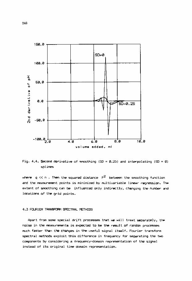
246

. 0

Fig. 4.4. Second derivative of -thing (SD = 0.25) and interpolating (SD = 0)

spl in-

where q << n . Then the squared distance F2 between the smoothing function

and the measurment points is minimized by rmltivariable linear regression. The

extent of smoothing can be influenced only indirectly, changing the number and

locations of the grid points.

Apart from some special drift processes that w e will treat separately, the

noise in the measurements is expected to be the result of random processes

rmch faster than the changes in the useful signal itself. Fourier transform

spectral methods exploit this difference in frequency for separating the two

components by considering a frequency-domain representation of the signal

instead of its original time domain representation.

247

4.3.1 Continuous Fourier transformation

The frequency domain representation F of a function f depending on

time t is defined by the Fourier transform

m

kCf1 = F(Y) = s f(t)exp(-iZllYt)dt , -m

(4.31)

where i =(-l)”’ and F depends on the frequency Y. If the integral in

(4.31) converges, then the Fourier transform is one-to-me, and its inverse is

given by

The generally complex function

parts according to

F can be decomposed into real and imaginary

m m

F ( v ) = s f(t)cos(ZIbt)dt - is f(t)sin(2llvt)dt -m -m

(4.33)

due to the Euler equality expcix) = cos(x) + i sin(x). If f is even, then

its transform F is real, F(v) = Re F(v). If f is odd, then F is

plrely imaginary, F(Y) = i Im F(v). Otherwise F is a complex valued function.

Sane elementary properties of the Fourier transform are listed in Table 4.3.

Table 4.3 Properties of the Fourier transform

Property Relationship

1 ineari ty ZCa1f1 + azf21 = a1ECfyI + a2ZCf21

time shifting ZCf(t-to)l = FCf(t)lexp(-i2nvt0)

differentiation IC--fl = i2n~ZCfl d

dt

integration Z[ s mf(7)d7 3 = (iZn~)-~ZCfl -m

248

It is important that differentiation and integration in the time domain give

multiplication and division, respectively, by the variable v in the

frequency domain. The role of convolution integrals will be further discussed

in Chapter 5.

We can regard Fourier transform as decomposing f into trigonometric

functions of different frequencies. This spectral decomposition is based on the

property

m 1 ~ ~ ( z n v l t ) i = A ~ E ~ ~ - ~ ~ ) + 6(r+v1)1 (4.34)

where 6(v-vl) denotes the Dirac impllse such that 6(v-vl) = 0 for v f u1

and

(4.35)

By the time shifting property shown in

cosine function

Table 4.3, the transform of a shifted

The transform (4.36) is complex valued and vanishes at all frequencies except

v = r1 and v = -v l . The complex number F C v I can be represented by its

amplitude A(v) = CRe%(v) + Im2F(v)11'2 and phase

P ( V ) = arc tg [Im F(v)/Re F(v)]. ck functions of v , A ( v ) and ~ ( v ) are

called amplitude and phase spectra, respectively. In the amplitude spectrum of

(4.36) we have ~ ( 7 ~ ) = ~ ( - v ~ ) = h1 , whereas ~ ( v ) = 0 if I v I IC v1 . Since any piecewise continuous function can be expanded into a sum of trigonometric

functions with different amplitudes and phases, by (4.36) and by the linearity

of Fourier transform the amplitude and phase spectra A ( v ) and ~ ( v ) uniquely

specify the function

only as the power spectrum $ ( v ) = Re%(") + Im%(v) , which does not specify f uniquely, but contains sufficient information in many applications.

f. The frequency domain description is frequently given

This is the analytical formalism we will need in the present section. The

experimental data are, however, almost invariably given by a limited set of

discrete observations instead of a continucus function defined for -m < t < m.

The next s u m t i o n extends the Fourier transformation to a finite set of

sampled data.

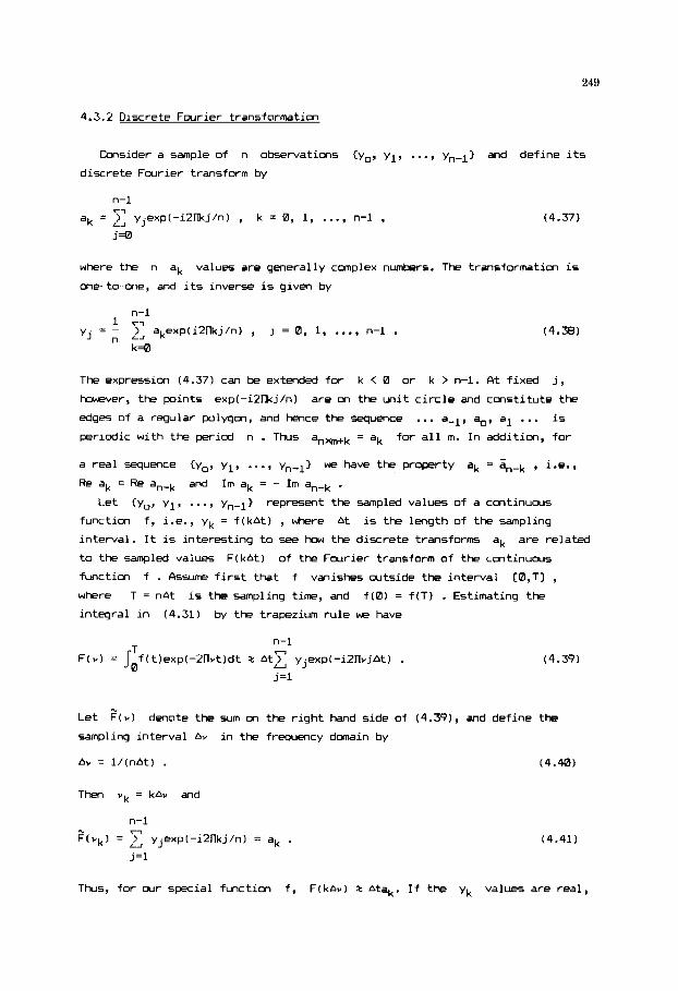
249

4.3.2 Discrete Fourier transformation

Consider a sample of n observations {yo, y1, ..., yn-l> and define i t 5

discrete Fourier transform by

n-1 Tl

L A ak = ) yjexp(-i2nkj/n) , k = 0, 1, ..., n-1 ,

j=Q,

(4.37)

where the n ak values are generally complex numbers. The transformation i s

one-to-one, and i t s inverse i s given by

n-1

2, akexp(i2nkj/n) , k=O

1 Tl

yj = ; j = 0, 1, ..., n-1 . (4.38)

The expression (4.37) can be extended fo r k < 0 or k > n-1. A t f ixed j,

however, the points exp(-iZmj/n) are on the unit c i r c l e and constitute the

edges of a regular polygon, and hence the sequence

periodic with the period n . Thus a n m k = ak fo r a l l m. I n addition, for

a real sequence {yo, yl, ..., yn-l} we have the property dk = +,-k , i.e.,

Re ak = Re anWk

... a-1, do, a1 ... i s

and I m ak = - I m an-k . Let {yo, yl, ..., yn-l} represent the sampled values of a continuous

function f, i.e., yk = f ( k A t ) , where A t i s the length of the sampling

interval . It i s interesting t o see how the discrete transforms dk are related

t o the sampled values F(kAt) of the Fourier transform of the continuous

function f . Assume f i r s t that f vanishes outside the interval C0,Tl , where T = nAt is the sampling time, and f ( 0 ) = f ( T ) . Estimating the

integral i n (4.31) by the trapezium ru le we have

n-1 T

F ( v ) = J0f(t)exp(-2nvt)dt 2 At): yjexp(-i2nVjAt) . j=1

(4.39)

Let ? ( Y )

sampling interval Av i n the frequency domain by

AV = l / (nA t ) . (4.40)

denote the s u m on the r i gh t hand s i d e of (4.391, and define the

Then vk = kAv and

n-1 -.. Tl F(vk) = 2, yjexp(-i2nkj/n) = ak .

j=1

(4.41)

Thus, for cur special function f, F(kAv) z Atak. I f the yk values are real,

250

then by (4.40) the points of the dixrete spectrum are obtained at the

frequencies = 0 , v1 = 1 / T , v2 = 2/T, ..., vnI2 = n/(2T) , where vnI2

is called the Nyquist critical frequency. The further points of the spectrum

are determined by the relation

additional information. an-k = ak , and hence do not offer any

kwever, unless special care is exercised, generally the dixrete spectrum

does not estimate very well the sampled continuous spectrum. The problems we

face are as follows.

Aliasing is present if the function

a frequency Y higher than Y,,,~, say Y = vnI2 + &. This component shows up in the spectrum at the frequency

distorted unless f i5 bandwidth limited to less than the Nyquist

critical frequency. This relationship is the sampling theorem implying that

the sampling interval At shauld be chrxen sufficiently small, depending

on the estimated bandwith of f.

f contains a periodic component with

vnI2 - AY. Thus the spectrum is

Broadening and "leakage" of the spectrum is the consequence of the finite

interval [0,T] of integration in (4.39), if f does not vanish outside

this interval. In fact, (4.39) then means estimating the Fourier transform

of the product

defined by

f(t)WCm,Tl, where WCO,T] is the square window function

(4.42)

Thus Atak 2 PCfWC0,T13, which is the convolution integral of the

transforms ZCfl and Z[Wc0,T~3. The latter has rather unpleasant

properties. For example, Fig. 4.5 shows the even square window

and its

similar sidelobs. The undesired convolution of ZCfl with such a boxcar

function implies that the spectrum is broadened and has several sidelobs

near the critical frequency Y ~ , ~ . It can be improved by increasing the

samDle size.

WC-T,TI (purely real) transform. NWC0,T33 i5 caplex valued, but has

CIlthough one has to deal with the above problems, the discrete Fourier

transformation is still a powerful tool, mainly because of its numerical

efficiency. The efficiency does not follow from (4.37) that requires n2

complex multiplications. As shown, however, by Cooley and Tukey (ref. 141, the

transform can be computed in operations with an ingenious algorithm

called Fast Fourier Transformation (FFT). The original Radix-2 version of FFT

applies to sample sizes n = 9 , where m is a positive integer. This

nxlogp

251

assumption i s not very restr ict ive, since we can always add a suf f ic ient number

of zeros to the sample i n order to reach the nearest power of 2. As w e w i l l

discuss, such zero addition might even improve the spectrum.

sin2T9Q F(3) = - I

I I I 1 I---

Fig. 4.5. The boxcar function f ( t ) = WC-T,T3 and i t s Fourier transform F ( v )

The following module i s b a d on the FORTRAN program of Cooley, Lewis and

Welch (ref . 15).

Proqram module M67

6 7 8 0 REtl t t t t l ~ l ~ ~ l l l l l l l l l l l l $ l l l ~ l l l l l l ~ l l l ~ ~ l ~ ~ ~ ~ ~ l l l l l ~ ~ 6 7 8 2 REM I FAST FOURIER TRRNSFORH I 6 7 8 4 REH I RADIX-2 ALGORITHM OF COOLEY AND TUKEY t 6 7 0 6 RE! l l l l l l l l l ~ l ~ ~ $ l l ~ l ~ l l l l l l ~ l l l ~ l l ~ l l l l l l l l ~ ~ l l ~ l ~ l ~ ~

6 7 1 8 REtl tl LOK'(NLltlBER OF POINTS) 6712 REH A(1 ... 2.1, 6 7 1 4 REH B(1. . .2*tl) b 7 1 5 RER I N I D E N T I F I E R OF INVERSE TRANSFORMATION 6 7 1 8 RE! 0 - DIRECT TRANSFORMATION 6 7 2 0 REH NOT 0 - INVERSE TRANSFORMATION 6722 REH OUTPUT: 5 ? 2 4 REtl A(1. I .2*tli REAL PART OF TRANSFORNED SEQUENCE 6 7 2 6 REll B(1.. .2*ti) IHA61NARY PART OF TRANSFORHED SEQUENCE

6788 RER INPUT:

REAL PART OF FUNCTION VALUES IHRGINARY PART OF FUNCTION VALUES

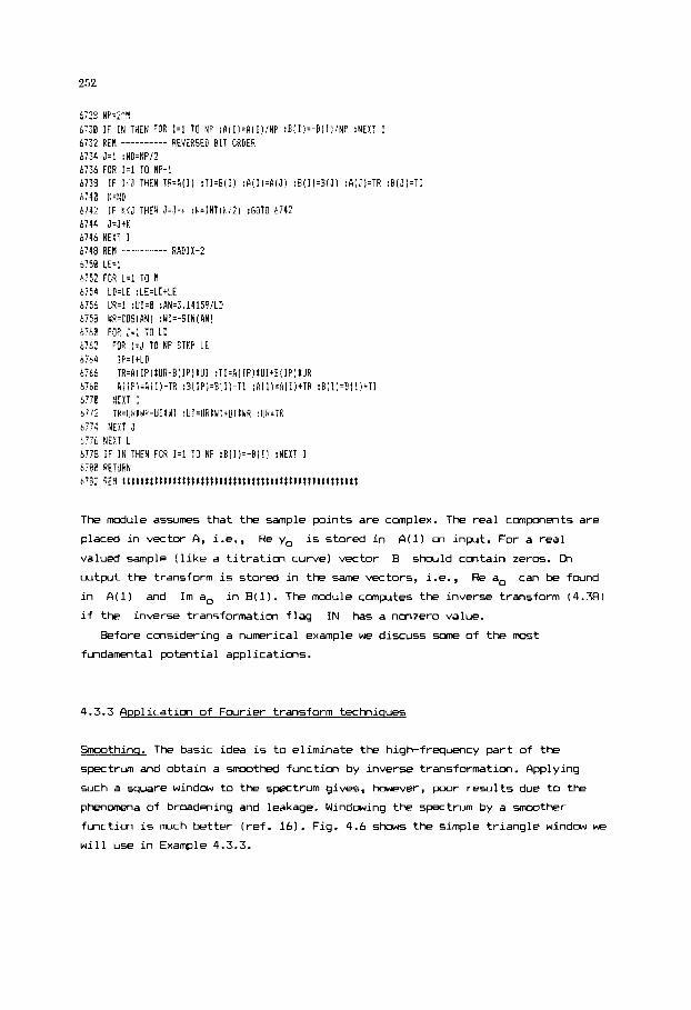
252

The module assumes that the sample points are complex. The real components are

placed in vector A , i.e., Re yo is stored in Q(11 on input. For a real

valued sample (like a titration curve) vector B should contain zeros. Cn

cutput the transform i5 stored in the same vectors, i.e.,

in A ( 1 ) and Im a, in B(1). The module compltes the inverse transform (4.38)

if the inver- transformation flag I N has a nmzero value.

Re a, can be found

Before considering a numerical example we discuss me of the m s t

fundamental potential applications.

4.3.3 Qpplication of Fourier transform techniques

Sroothinq. The basic idea is to eliminate the highfrequency part of the

spectrum and obtain a smoothed function by inverse transformation. Applying

such a square window to the spectrum gives, hDwever, pDOr results due to the

phenomena of broadening and leakage. Windowing the spectrum by a smoother

function is mch better (ref. 16). Fig. 4.6 shows the simple triangle windrw we

will use in Example 4.3.3.

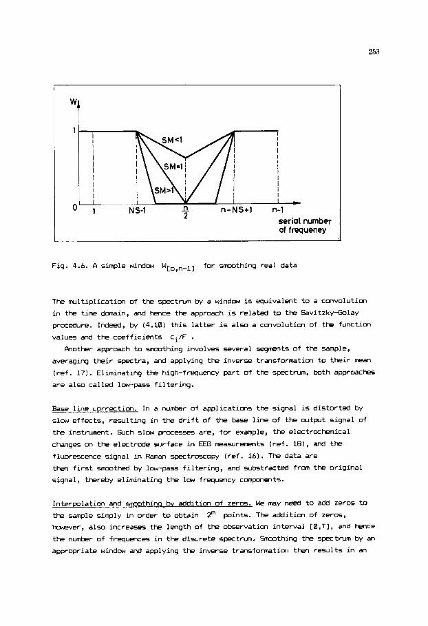
253

r I I I I I I I I I I I I I -

n-NS+1 n-1 z N S-1 serial number of frequeney

Fig. 4.6. A simple window Wro,n-ll fo r smoothing real data

The mult ip l icat ion of the spectrum by a window i s equivalent t o a convolution

i n the t i m e d m i n , and hence the approach i s related t o the Savitzky-Golay

procedure. Indeed, by (4.10) th i s l a t te r i s also a convolution of the function

values and the coeff ic ients ci/F . Another approach to smoothing involves several W m t s of the sample,

averaging the i r spectra, and applying the inverse transformation t o the i r mean

( re f . 17). Eliminating the high-frequency part of the spectrum, both approaches

are also called low-pass f i l t e r i ng .

Base l i ne correction. I n a number of applications the signal i s distorted by

slow effects, resulting i n the d r i f t of the base l i n e of the output signal of

the instrument. Such slow processes are, f o r example, the electrochemical

changes on the electrode surface i n EEG measurements ( re f . la), and the

fluorescence signal i n Raman spectroscopy (ref . 16). The data are

then f i rs t smoothed by low-pass f i l t e r i ng , and substracted f rom the or ig ina l

signal, thereby eliminating the low frequency cmpcnents.

Interpolation and smoothins by addition of zeros. We may need t o add zeros t o

the sample simply i n order t o obtain

however, also increases the length of the observation interval [0,T], and hence

the number of frequences i n the discrete spectrum. Smoothing the spectrum by an

appropriate window and applying the inverse transformation then resul ts i n an

p i n t s . The addition of zeros,

254

enhanced sample with new d a t a p o i n t s between the o r i g i n a l ones.

D i f f e r e n t i a t i o n and i n t e a r a t i o n . As seen from Table 4.3, we can e s t i m a t e the

d e r i v a t i v e of t h e sampled funct ion i f we mul t ip ly ak by t h e f a c t o r ( i 2 l l k A v )

before the inve r se t r ans fo rma t im. Th i s operation a m p l i f i e s the high frequency

components, and hence it can be used only with a smoothing window as a f u r t h e r

r ru l t i p l i e r . Ch the other hand the spectrum is divided by the same f a c t o r i n

o rde r to e s t ima te t h e i n t e g r a l of t h e sampled funct ion. Therefore , a t

s u f f i c i e n t l y l a r g e values of k

the i n t e g r a t i m . Th i s shows why i n t e g r a t i o n always l eads to sane smoothing.

the high-frequency components does n o t d i s t u r b

Munerical deconvolution. A number of techniques t h e o r e t i c a l l y r e s u l t i n l i n e

spectra, with n m z e r o va lues only a t well def ined va lues of t h e independent

va r i ab le . Due to s c a t t e r i n g phenomena, however, the s e p a r a t e l i n e s are

broadened i n t o p e a k s of a cont inuous cu rve that may be viewed as the

convolution of t h e o r i g i n a l l i n e spectrum with the Gaussian funct ion

g ( t ) = exp(-atZ) ( r e f . 16). By the last r e l a t i o n i n Table 4.3 we can restore

the t h e o r e t i c a l l i n e s t r u c t u r e , or a t least s i g n i f i c a n t l y narrow the p e a k s by

d iv id ing the transform of the ou tpu t s i g n a l by the transform of the Gaussian

and then performing inve r se t ransformation. Th i s procedure is of cons ide rab le

importance i f t h e p e a k s ove r l ap and t h e i r number is n o t a p r i o r i k n m .

Feature e x t r a c t i o n and d a t a reduct ion. A sampled cont inuous s i g n a l can

f r equen t ly be well descr ibed i n terms of a few l awf requency components of its

d i s c r e t e Four i e r transform. Th i s enab le s u s to s tudy , store and compare

r e l a t i v e l y s h o r t v e c t o r s i n l a r g e d a t a bases.

Example 4.3.3 Detection of end p o i n t s i n po ten t i cme t r i c t i t r a t i o n by Four i e r

transform techniques

Cur goal is again to f i n d the maxima of t h e smoothed first d e r i v a t i v e of the

t i t r a t i o n curve f i r s t s tud ied i n Example 4.1.3. Recal l that t h e d i s c r e t e

transform of a real sample s a t i s f i e s the r e l a t i o n s h i p

j = 1, 2, ..., n/2-1 . an/2+j = Sn/2-j f o r a l l

h l t i p l y i n g t h e transform by the window Wco,n-13 show, i n Fig. 4.6 t h i s

property i s . p r e s e r v e d , and hence the i n v e r s e t ransform of t h e product is purely

real. The window (or low-pass f i l t e r ) is desc r ibed i n terms of two parameters,

the index NS of the frequency w h e r e smoothing is s t a r t e d , and t h e smothing

f a c t o r SM that determines t h e slope of t h e decreasing part of t h e window as

show, on Fig. 4.6. The transform of the -tW funct ion is then the product

Z[f]Z;[W]. To ob ta in the smoothed d e r i v a t i v e of f , we mul t ip ly t h i s product by

255

the coeff ic ient (i2llkAv) and perform inverse transformatim, whereas the

smmthed curve i s the inverse transform o f the product itself.

The following main program includes the above steps.

180 REM

182 REW EX. 4.3.3 APPLICATION OF FFT TECHNIQUES I84 REH MERGE Hb7 186 REH ---------- DATA 188 REH (NUHBER OF POINTS) 118 DATA 5 112 RER (V,ml; pH1 114 DATA 2.4, 2.642, 2.6, 2.786, 2.8, 2.786, 3.0, 2.877 116 DATA 3.2, 2.9e6, 3 . 4 , 3.126, 3.6, 3.295, 3.8, 3.488 118 DATA 4.0, 3.659, 4.2, 3.816, 4.4, 3.952, 4.6, 4.874 128 DATA 4.8, 4.183, 5.8, 4.285, 5.2, 4.384, 5.4, 4.488 122 DATA 5.6, 4.579, 5.8, 4.682, 6.0, 4.791, 6.2, 4.9~8

126 DATA 7.2, 8.617, 7.4, 9.747, 7.6,18.134, 7.8,in.34e 128 DATA e . 8 , ~ . 491, e.2,1~.6~4, 8.4, 18.692, 8.6, 111.766

1 2 4 DATA 6.4, 5.845, 6.6, 5.211, 6.8, 5,444, 7.0, 5.859

200 REH ---------- READ DATA 282 READ W :N=2*N

286 FOR 1.1 TO N 208 READ Z(I),F(I) 210 A(I)=F(I) :B(I)=0 212 NEXT I : D X = I ( P ) - Z ( I ) 214 REM ---------- CALL FOURIER TRANSFORNATION MDDULE 216 I N 4 :6USUB 6706

SHOOTHING FROR THE NS-TH FREQUENCY 218 REM _ _ _ _ _ _ _ _ _ _ 220 RER Stl: SHOOTHIN6 FACTOR 222 NS=N/8 :SM=l 224 FOR 1.2 TO N / 2

228 IF S(B THEN S=B 238 M I )=S1A( I ) :B(I)=SkB( I) 232 A I N t 2 - I ) = A ( I) : B ( N t 2 - I )4( I ) 234 NEXT I 236 S=l -SR :IF S(0 THEN S.8 238 A ( N / 2 t l ) = A ( N / 2 t l ) tS

STORE SHOOTHED TRANSFORH 248 RER _ _ _ _ _ _ _ _ _ _ 242 FOR 1.1 TO N 244 U(I)=AIIl : V [ I ) = B ( I ) 246 NEXT I

INVERSE TRANSFORHATION 248 REH _ _ _ _ _ _ _ _ _ _ 250 IN=1 :6OSUB 6788 252 RE1 _____---__ STORE SMOOTHED FUNCTION VALUES 254 FOR 1.1 TO N :S(I)=A(I) :NEXT I 256 REM ---------- TRANSFOR1 OF THE F I R S T DERIVATIVE 2 5 8 D=6,28319/N/DX 268 All)=B :BI1)=0 262 FOR 1.2 TO N U t l

284 D I M I I N 1 IF i N ) 3 S I N 1 ,Dl N 1 A ( N ) B(N 1 ,U( N 1 , V ( N 1

226 S:I :IF I b N S THEN S=1-(ItI-NS)IINI2tZ-NS)tSH

264 A [ I )=-V[ I )tDt( 1-11 :B( 1 ):U( I ItDkI 1-11 266 A ( N t 2 - I ) = A ( I 1 : B ( N t Z - I ) = - B ( I ) 268 NEXT I 278 RER ---------- INVERSE TRANSFORMATION 272 I N = l :GOSUB 6788 3 4 REIl ---------- STORE DERIVATIVES 276 FOR 1.1 TO N :D(I)=A[I) :NEXT I

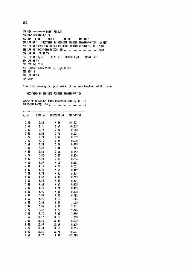
256

PRINT RESULTS 278 REn --________ 280 V$=STRING$[50,"-") 282 A)=n 1.11 ##.#I **.#I II#.llIB 284 LPRINT ' 2B6 LPRINT "NUMBER OF FREQUENCY WHERE SM@OTHING STARTS, NS . ,';NS 288 LPRINT nSHOOTHING FACTOR, SW . . . . . . . , , , . . . . . . . . . . . . . . . . . ';St! 298 LPRINT :LPRINT VS 292 LPRINT V, nl HEAS pH SHOOTHED pH RERIVITIVE' 294 LPRINT V I 296 FOR 1.1 TO N 298 LPRINT USING AS;Z(I) ,F(I),S[ I ) ,D( I ) 388 NEXT I 502 LPRINT V1 304 STOP

SMOOTHING BY DISCRETE FOURIER TRANSFORHATION": LPRINT

The following output should be evaluated with care.

SMOOTHING BY RISCRETE FOURIER TRANSFORHATION

NUMBER OF FREQUENCY YHERE SMOOTHING STARTS, NS , . 4 SWOOTHIN6 FACTOR, S i l I , , . . . . , . . . . . , . . , . , . , . , . , . , , 1

2.48 2.60 2.80 3.00 3.20 3.48 3.68 3.80 4.00 4.20 4.40 4.68 4.80 5.88 5.20 5.40 5.68 5.88 6.B0 6.20 6.40 6-60 6.80 7.80 7.20 7.48 7.60 7.80 8.00 8.20 8.48 8.60

2.64 4.44 -19.323 2.71 2.67 -0,319 2.79 2.81 -0.258 2.08 2.15 0.521 2.99 2.92 0,632 3.13 3,04 0.910 3.38 3.26 0.995 3.48 3.44 1.043 3.66 3.66 8 . 942 3.82 s -82 0.824 3.95 3.99 0.696 4.07 4.10 8.601 4.18 4.22 8.511

4.38 4.41 8.414 4.48 4.40 8.399 4.58 4.57 0.484 4.68 4.b5 8.438 4.79 4.74 0.485 4.91 4.85 8,610 5 - 8 5 4.98 0.782 5.21 5.19 1.244 5.44 5.47 1.935 5.86 b.36 7.811 8.62 8.29 9.506 9.75 9 .G 3.998

18.13 10.18 1.888 18.35 16.43 0.972 10.49 1B.64 0.619 18.60 18.61 -0 I 193 10.69 18.75 -0.287 10.77 8.99 -19.388

4.29 4.31 8-45?

257

Indeed, both the m t h e d curve and the derivative have sidelobs at both ends

of the sample, but the results are satisfying at most o f the internal points.

Since Fourier transform spectral methods are usually applied to samples much

larger than the one considered here, the distortion at a few outermost points

is not a serious drawback.

Exercise

Repeat the computations with other NS and SM values and investigate

how the number of maxima of the derivative changes.

4.4.1 Heuristic methods o f local interpolation

Spline interpolation is a global method, and this property is not

necessarily advantageous for large samples. Several authors proposed

interpolating forrmlas that are "stiffer" than the local polynomial

interpolation, thereby reminding spline interpolation, but are local in nature.

The cubic polyncmial of the form

(4.43)

has been used in the i-th interval by Akima (ref. 191, where

d = x - xi , hi = xi+l - xi , whereas the polynomial at d = 0 and d = hi, respectively. Cancatenation of the

polynomials (4.43) gives a continuous and once continuously differentiable

interpolating function. (Notice that cubic splines are twice continuously

differentiable.) The kuristics lies in the choice of ti . The weighted sum

ti and ti+l denote the derivative of

(4.44)

has been proved useful where

forrmlas have been suggested by Butland (refs. 20,Zl).

mi = (yi+l - yi)/hi . Slightly different

258

Exercise

0 Interpolate the titratim curve implementing Akima's method. Compare the

interpolating curve with the results of local cubic interpolation and spline

interpolation.

4.4.2 Praessins of spectroKoDic data

In order to maximize information obtained from raw spectroscopic data,

analytical chemists and instrumental specialists depend M signal processing

and apply a large number of specialized versions of the basic methods

considered in this chapter, as well as the parametric methods discussed in the

previous chapter, see, e.g. (ref. 22). Here we provide only an example of

parametric methods. Table 4.4 shows 20 points of the electronic absorption

spectrum of o-phenilenediamidine in ethanol (ref. 23) .

Table 4.4 Points of an electronic absorption spectrum

Absorptivity 20000 29020 3mz0 32002l lWQ#d 9002 &!?I00 &mil

Frequency, cm-I 4- 4 1 m 4waew 390C30 36000 3 7 m 3612U10 35QUGl

Absorptivity 6500 &!?I00 38mm 1800 Wil 950 1BZ0 27aM

Frequency, cm-I 340iU1 33007l 32202 31-

Absorptivity 3i00 2500 850 170

Following the treatment in (ref. 23) we separate the spectrum into 3

Gaussians, and estimate the parameters

function

Ai,Bi and Ci, i = 1, 2, 3, of the

y = L, T-l Aiexp[ -[ 3i;--L] - c. 2 ] i=l

(4.45)

using the nonlinear least squares module M45. The initial estimates of the

parameters shaKl in Table 4.5 can be obtained by inspecting the curve. Indeed,

Ci is the location of the i-th peak, Ai is its height and Bi is its

half-width multiplied by Jz . The initial estimates and the ones rwlting from the fit are sham in Table 4.5. The fit is plotted on Fig. 4.7.

259

Table 4.5 Parameter e s t i m a t e s i n model (4.45)

I n i t i a l

390m 2500

46wm 6500 2500 420m 3 m 2 w 34020

Final

37165 2365

4m46 64619 2754 42am 3369 1844 34434

95% confidence in te rva l

-106 - 44223 1946 - 2784 47774 - 48319 52Z0- 7588 2210 - 3299 41419 - 42741 2271 - 40ilH 1684- 2m3 34247 - J46MI

___l___________l_

a0

u o v e n u m b e r . l / c m

Fig. 4.7. O b s e r v e d (poin ts ) and f i t t e d (continuous) e l e c t r o n i c absorption

spectrum

Exercise

Use smoothing s p l i n e to obtain the i n i t i a l e s t i m a t e s f o r peak locat ion ( t h e

l o c a t i m of the m a x i m u m ) , peak height ( funct ion value a t t h e maximum poin t )

260

and half-width (the distance between the maxirmm point and the inflection

point).

REFERENCES

1 2

3

4 5

6

7

8

9 10 11 12

13

14

15

16

17

18

19

20

21

22

23

S.M. Bozic, Digital and Kalman Filtering. Arnold, London, 1979. H.C. Smit, Specification and Estimatim of Noisy Fhalytical Signals, Laboratory of Pnalytical Chemistry, University of Amsterdam, 1986, (manuscript) A. Ralston, A First Course in krwrical Chalysis, McGrawf-lill, New York, 1965. P. Henrici, Elements of Numerical Analysis, John Wiley, New York, 1964. F. B. Hildebrand, Introduction to Numerical Analysis, McGraw-Hill, New York, 3956. V.P. Glushko (Editor), Thermodynamic properties of Individual Substances, (in 4 vol-) Nauka, MOsccw, 1978-1982 (in Russian) A. Savitzky and M.I.E. Golay, Smoothing and differentiation of data by simplified least squares procedures, Analytical Chemistry, 36 (1964) 1627-1639. J. Steiner, Y. Fermonia and J. Deltour, Comment on smwthing and differentiation of data, Fhalytical Chemistry, 44 (1972) 1906-1909. A. Prator and P.M.A. Sherwood, Fhalytical Chemistry, 52 (1980) 2315. J. Wzi, Eotvos Lordnd University Budapest, Personal cmication. C. de Bwr, P Practical Guide to Splines, Springer, New York, 1978. I.J. Scbenberg, On interpolation by spline functions and its minimal properties. Ch Approximation Theory, p109. Proceedings of the Conference held in the Mathematical Research Institute at Oberwolfach, Black Forest, August 4-10, 1963. Birkhaser, Basel-Stuttgart, 1964. C.H. Reinxh, Smoothing by spline functions 1-11. Numerische Mathematik, 10 (1967) 177-183 and 16 (1971) 451-454. J.W. Cmley and J.W. Tukey, An algorithm for the machine calculation of cmplex Fourier series, Mathmatics of Compltation, 19 (1965) 297. J.W. Cmley, P.A. Lewis and P.D. Welch, The fast Fourier transform and its aoolications. in K. Enslein. A. Ralston and H.S. Wilf (Editors) ~. , , Statistical Methods for Digiial Computers, Vol. 3, 1977.

John Wiley,'New York,

R.R. Griffitk (Editor), Transform Techniques in Chemistry, Plenum Press, New York, 1978. P.D. Welch, The use of fast Fourier transform for t k estimation of pcwer spectra: A method based on time averaging over short, modified periodigrams. IEEE Trans. Audio and Electroacustics. W-15 (1967) 70-73. J. Berkhwf and B.O. Walter, Temporal stability and individual differences in human EEG. An analysis of variance of spectral values. IEEE Trans. B i d . Engng. 15 (1968) 165-173. H. Akima, A new method of interpolation and smwth curve fitting based cn local procedures. Journal of the Aa'l, 17 (1970) 589-bal2. I. Butland, in K.W. Brodie (Editor) IMA Conf. on Mathwnatical Methcds in Cmp. Graphics and Design '79. Academic Press, Toronto, 1960. R.I. Tervo, T.I. Kenett and W.V. Prestwich, An automated background estimation procedure for gamma ray spectra. b c l . Instr. Meth. Phys. Res., 216 (1983) 205-ZB. P. Gaus and I.B. Gill, Smoothing and differentiation of spectroxopic curves using spline functions, J. Applied Spectroscopy, 38 (1984) 37E-376. G. Beech, F W T R W IV in Chemistry, John Wiley, New York, 1975.

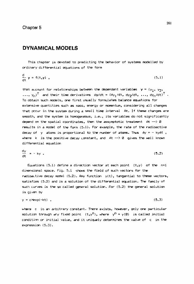
Chapter 5 261

DYNAMICAL MODELS

This chapter is devoted to predicting the behavior of systems modelled by

ordinary differentidl equations of the form

d -- y = f(t,y) , (5.1) dt

that account for relationships between the dependent varjables

..., yn)T To obtain such models, one first usually formulates balance equations for

extensive quantities such as mass, mergy or momentum, cmsidering all changes

that occur in the system during a mall time interval At. If these changes are

smooth, and the system is homogenecus, i.e., its variables do not significantly

depend on the spatial coordinates, then the assymptotic treatment At -> 0

results in a rodel of the form (5.1). For example, the rate of the radioactive

decay of y atans is proportional to the number of atoms. T b s Ay = - kyAt , where k is the positive decay constant, and At -> 0 gives the well know

differential equation

y = (yl, y2, and their time derivatives dy/dt = (dyl/dt, dy2/dt, ..., dy,/dtlT .

( 5 . 2 )

Equations (5.1) define a direction vector at each point (t,y) of the n+l

dimensional space. Fig. 5.1 shows the field of such vectors for the

radioactive decay rodel (5.2). Fhy function y(t), tangential to these vectors,

satisfies (5.2) and is a solution of the differential equation. The family of

such curves is the so called general solution. For ( 5 . 2 ) the general solution

is given by

y = c*xp(-kt) , (5.31

where c is an arbitrary constant. There exists, howwer, m l y one particular

solution through any fixed point (t,yo), where yo = y(0) is called initial

condition or initial value, and it uniquely determines the value of c in the

expression (5.3).

262

\ \ \ \ \ \ \

t

Fig, 5.1. Vector field defined by the differential equation

Existence and uniqueness of the particular solution of (5.1) for an initial

value

sufficient to a55ume that the functim f is differentiable and its

derivatives are bounded. Except for a few simple equations, however, the

general solution cannot be obtained by analytical methods and we must seek

numerical alternatives. Starting with the knom point

methods generate a sequence (tl,y'), (t2,p), ..., (ti,yi), approximating the points of the particular solution through

large and we shall be content to outline a few popular types. [he of them will

deal with stiff differential equations that are very difficult to solve by

classical methods. Related topics we discuss are sensitivity analysis and quasi

steady state approximation.

p can be s h under very mild assumptions. For example, it is

(to,p), all nwrical

(to,p). The choice of the method is

Both the function f and the initial condition p may depend on unknown

parameters p :

d

dt -- y = f(t,y,p), y ( 0 ) = P(P) . (5.4)

263

.*

A frequent problem is to estimate p from the sample { (ti,yi),

i = 1, 2, ..., nm 1, where yi denotes an error-corrupted observation of the

solution. If the solution is known in analytic form, we have a parameter

estimation problem treated in Chapter 3. In principle, one can use the wne

methods even without an analytical solution, solving the differential equations

numerically in each iteration of the estimation procedure. The canputational

cost of such treatment is, hmever, too high for most personal canputers, and

we will propose a special technique with improved numerical efficiency.

.*

Modeling of saw systems leads to higher order differential equations of the

form

,(m) = f(t,y,y(l) ,..., y(m-1)) . (5.5)

The additional variables

a set (5.1) of m first-order differential equations, and hence you do not

need special methods to solve (5.5). Nevertheless, we will treat separately the

problems of identifying and inverting single-input, single-cutput linear

systems described by the equation

y(m) + aly(m-l) + ... + amy = blu(m-l) + ... + bmu ,

xi = y, x2 = y(l), . . . , xm = y(m-ll reduce (5.5) to

(5.6)

where u(t) is the input and y(t) is the output of the system.

Ordinary differential equations are suitable only for describing horogenwus

systems, and we need partial differential equations if the variables depend

also on spatial coordinates. The solution of such equations is beyond the x o p e

of this b w k .

5.1 W R I W SDLUTICN IF ORDINPRY DIFFEREMIa ECXKSTIauS

Although not r e c m d e d for practical use, the classical Euler

extrapolation is a convenient example to illustrate the basic ideas and

problems of numerical methods. Given a point (ti,y') of the numerical

solution and a step size h, the explicit Euler method is based on the

approximation

to ti+l = ti + h by the expression

(yi+' - y(i))/(ti+l - ti) 5 dy/dt to extrapolate the solution

yi+l = y1 ' + hf(ti,y') . (5.7)

ck seen fran Fig. 5.2, reducing the step size h improves the accuracy of

this estimation.

264

Fig 5.2. True values y ( t ) and cmprted values y(i) i n the Euler method

While i n the f i r s t step the deviation from the exact solution stems only from

approximating the solution curve by i t s tangent l ine, i n further steps we

calculate the Slope a t the current approximation instead of the unknown

true value y(ti), thereby introducing additional errors. The solution o f

(5.2) is given by (5.31, and the to ta l error E i = y(ti) - yi f o r t h i s

simple equation i s

yi

Ei = y(ti-l)exp(-kh) - (1 - kh)yi-l . (5.8)

Since yi-l = y(ti-l) - Ei-l , (5.8) yields the recursive re la t ion

Ei = [exp(-kh) - (1 - kh)ly(ti-l) + (1 - kh)Ei-l . (5.9)

The f i r s t term i n (5.9) i s the local truncation or step error that occurs i n

a single step and does not take i n t o accwnt the use of

y ( t i - 1 ) . The second term shows the propagation of the error

primary importance to keep the ef fect of

resulting i n the s t a b i l i t y of the method. I n t h i s simple example the

yi-' instead o f

Ei-l. It i s of

Ei decreasing i n l a t t e r steps,

265

requirement of stability implies 11-khl 5 1 , 50 that

(5.10) 2

k h < - .

Thus, stability can be achieved only at sufficiently small step sizes. Such

steps decrease also the truncation error, but increase the required

computational effort. Therefore, a c m goal of all numerical methods is to

provide stability and relatively small truncation errors at a reasonably large

step size (refs. 1-2).

The stability of the Euler method is improved by using interpolation instead

of extrapolation, and considering the tangent evaluated at ti+l :

yi+l = yi + hf(ti,yi+') . (5.11)

For the special case of (5.2) we can solve (5.11) as

and then the total error is given by

1 y(ti-l) + (5.12)

1 + kh 1-1 '

The truncation errors in (5.9) and (5.12) are of the same magnitude, but

the implicit Euler method (5.11) is stable at any positive step size h. This

conclusion is rather general, and the implicit methods have improved stability

properties for a large class of differential equations. The price we have to

pay for stability is the need for solving a set of generally nonlinear

algebraic equations in each step.

To compare the explicit and implicit Euler methods w e exploited that the

solution (5.3) of (5.2) is known. We can, howwer, estimate the truncation

error withwt such artificial information. Considering the truncated Taylor

series of the solution, for the explicit Euler method (5.7) we have

(5.13)

where we assumed

of 8 is between ti and ti+l, but otherwise unknown. Nevertheless, (5.13)

shows that the truncation error is proportional to

expression for each method, and express the truncation error in the form

CXhP+' , where the integer explicit and implicit Euler methods are both first order ones. While a higher

order implies smaller truncation error, this does not necessarily mean improved

yi = ~ ( t ~ - ~ ) to obtain the local truncation error. The value

h2. We can derive a similar

p is said to be the order of the method. The

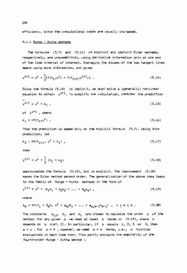
266

efficiency, since the cmpltational costs are usually increased.

5.1.1 Runse - Kutta methods

The formulas (5.7) and (5.11) of explixit and implicit Euler methods,

respectively, are unsynmetrical, using derivative information only at me end

of the time interval of interest. Averaging the Slopes of the two tangent lines

means using m r e information, and gives

h

2 yi+l = yi + -[f(tiryi) + f(ti+l,yi+ql . (5.14)

Since the formula (5.14) is implicit, we must solve a (generally) nonlinear

equation to obtain

yi+l = Y’ ’ + kl 3

yi+’. To simplify the calculation, consider the prediction

- (5.15)

of yi+l , where

kl = hf(ti,y’) . (5.16)

Thus the prediction is based only on the explicit formula (5.7). Using this

prediction, let

approximates the formula (5.14), but is explicit. The improvement (5.18)

makes t k Euler method second order. The generalization of the above idea leads

to the family of

yi+l = yi + (blkl

where

km = hf (ti + dmh,

Runge - Kutta methods in the form of

+ $k2 + ... + bsks) ,

y’ + amlkl + ... + am,,lk,ll , 1 5 m s .

(5.19)

(5.20)

The constants aij, bi and di are chosen to maximize the order p of the

method. For any given p we need at least 5 terms in (5.191, where s

depends on p (ref. 2). In particular, if p equals I, 2, 3 or 4, then

s = p . For p = 5 , however, we need s = 6 terms, i.e., 6 function

evaluations in each time step. This partly explains the popllarity of the

fourth-order Runge - Kutta method :

yi+l = yi + kl/6 + k2/3 + k3/3 + k l / 6 ,

where

kl = hf ( ti,yl)

k2 = hf( t i + h/2, y l + kl/Z)

k3 = hf ( t i + h/2, yi + k2/2)

k4 = hf ( ti + h, y1 + k3/Z) .

267

(5.21)

(5.22)

The following program module extends the formula (5.21) t o vector

d i f ferent ia l equatims of the form (5.1), simply by considering y , f and

ki as vectors.

Prosram module M70

7000 REH ttttttttttttttttttttttt~ttttttttttttttt~ttttttttttt 7P02 RE1 t SOLUTION OF ORDINARY DIFFERENTIAL EQUATIONS t 7004 REN t FOURTH ORDER RUNGA-KUTTA IIETHOD t 70C6 REM t t t t t t t t t t t t ttttt t t t t t t tt t t t t t t t ttttt8tttt t t t ttt t t t 7188 REIl INPUT: 70lB RE! N NURPER OF DEPENDENT VARIABLES 7012 HEM T INITIAL TIIE 7814 REII Y(N1 INITIAL CONDITIONS 7016 REN H TINE STEP SIZE 7018 RER NS REQUIRED NUHRER OF STEPS 7028 REH OUTPUT: 7822 REn T END TINE 7024 REII Y(N1 SOLUTION AT END TINE 70% RE! USER SUPPLIED SIIBROUTINE: 7028 REN FRO! LINE 900: T,Y(N) --> DINj I RHS EVALUBTION ) 7030 REM bUYILIAFiY ARRAYS: 7032 REM R(N),Q(N) 7034 FOR L = l TO NS 7 0 2 FOR I=1 TO N :R(ll=Y(I) :NEXT I 7C38 GOSUP 900 7040 FOP 1.1 TO N :QII!=D(II :Y(I)=R(IIt,StHtD(II :NEXT I 7042 T=T+.StH :GOSUB 900 7844 FOR I=1 TO Y :QII)=Q(I)t?tD(I) :Y(I)=R(I)t.5tHtDiI) :NEXT I 7046 60SUB 900 7048 FOR I=l TO N :QlIl=QIIl+~tD(Il :Y(I)=R(IjtHtD(I) :NEXT I 7050 T=Tt.StH :GOSUB 900 7852 FOR 1.1 TO N :YII!=R(I)tHi6t(Q(I]tD(I)) :NEXT I 7054 NEXT L 7156 RETURN 7058 REH ttttt~tttttttttttttt~ttttttlttttttttttttttttttttFt~

The module ca l l s the user supplied subroutine start ing a t l i n e VDZl that

evaluates the r i gh t hand sides of (5.1) a t the current values of the Y

vector and t ime T and put them i n t o the vector D. For a single equatim only

Y ( 1 1 and D(1) are used. The step size H and the number NS of steps are

selected by the user.

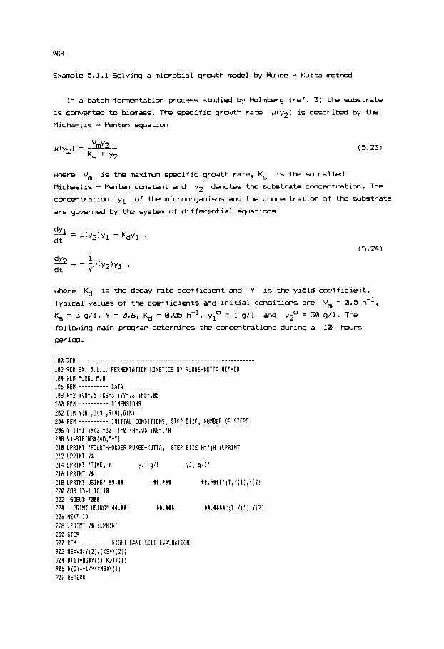
268

Example 5.1.1 Solving a microbial growth model by Runge - Kutta method

In a batch fermentation process studied by Holmberg (ref. 3) the substrate

is converted to biomass. The specific growth rate

Michaelis - Menten equation u(y2) is described by the

(5.23)

where Vm is the m a x i m specific growth rate, K, is the so called

Michaelis - Menten constant and yz

concentration y1

are governed by the system of differential equations

denotes the substrate concentration. The

of the microorganisms and the cmcentration of the substrate

(5.24)

where Kd is the decay rate coefficient and Y is the yield coefficient.

Typical values of the coefficients and initial conditions are

K, = 3 g/1, Y = 0.6, Kd = 0.05 h-', yl0 = 1 g/l

following main program determines the concentrations during a 10 hours

period.

Vm = 0.5 h-',

and yZo = XI g/l. The

100 REb _.._____________________________________-----.-.-----------

1 0 2 REN EX. 5.1.1. FERMENTATION K I N E T I C S BY RUNGE-IUTTA NETHOD 104 REM bER6E I70 106 REN ---------- DATA 108 N=? :Vfl=.5 :G=3 :YY5.6 :liD=.05

3 2 D I M Y(N! ,D(N! ,R(NI ,CI INI 204 REH ---------- I N I T I M CONDITIONS! STEP S I Z E , NUIBER OF STEPS 28t Y ( l ) = l : ? ( 2 ) = 3 0 :T=8 :H=.E: ;FiS=l!H 208 V I 4 T R I H 6 P I 4 0 , "-"! 210 LPRINT "FOURTH-ORDER RUNGE-KUTTA, 2!2 LPRINT V4

2 1 6 LPHINT VO :I8 L P K N T U S I N 6 " 11.11 220 FOR !D=l TO 18

224 L F R l N T USINGn tU,R# HR.#l# t t . t # t U " : T , V ( l ! ,Y[2) 226 N E l T I D 228 LF'R!IT \'I : P R I N T 2 0 STUP 5 P 0 RE\ ---------- RIGHT HAND SIDE EVALUATION 902 NS=Vl??Y(Z)!(ES+Y[2! 1

:at REM ---------- DII~EWNS

STEP S I Z E H=";H :LPRINT

214 LPRINT " T I H E , h Y f , !I1 c, g l l "

xw * X#t tU. tUUt" ;T,Y ( 1 1 , Y ( 2 !

m GOSUB 7100

704 D ( 1 ! ~ M S t Y [ l ) - Y D t Y ! l ) 906 D i ? ) = - l ! Y Y t M S t Y ( l ) 908 RETURN

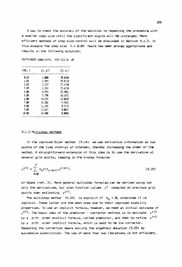
269

A way to check the accuracy of the solution is repeating the procedure with

a smaller step size until the significant digits will be unchanged. More

efficient methods of step size cmtrol will be discussed in Section 5.1.3. In

this example the step size

results in the following solution:

h = 0.05 hours has been proved appropriate and

FOUPTH-ORDER RUNGE-KUTTk, STEP SIZE H z .05

T I t l E , h

0.00 1.00 z.00 3.08 4.00 5.00 t.OO 7.00 8.00 9.00

10.00

1.000 1.498 2,239 3.339 4.955 7 , 2P0

10.524 14.586 15.264 15.557 14.800

30.0000 29.0678 27.6780 25.b158

18.1852 12.0600 4.5845 0.2518 8.0033 0.0100

22. sem

5.1.2 Multistep methods

In the improved Euler method (5.14) we use derivative information at two

points of the time interval of interest, thereby increasing the order of the

methal. A straightforward extension of this idea is to use the derivative at

several grid points, leading to the k-step formulas

( 5 . 2 5 )

of &lams (ref. 2). More general rmltistep forrmlas can be derived using not

only the derivatives, but also function values

points when estimating yi+l. yi computed at previcus grid

The multistep method (5.25) is explicit if b,, = 0, otherwise it is

implicit. These latter are the test ones due to their improved stability

properties. To use an implicit formula, haever, we need an initial estimate of

yi+l. The basic idea of the predictor - corrector methods is to estimate yi+l

by a p-th order explicit formula, called predictor, and then to refine yi+l

by a p-th order implicit formula, which is said to be the corrector.

Repeating the correction means solving the algebraic equation ( 5 . 2 5 ) by

successive substitution. The use of m r e than two iterations is not efficient.

270

The great advantage of the predictor - corrector methods i s that i n addition

t o yi+l, i n expression (5.25) we need only previously computed (and saved)

function values. Thus, the computational cost depends on the number of

corrections and does not depend m the order p of the part icular forrmla.

Starting a rmlt istep method i s an additional problem, since no previcus

funct im values are yet available. One can s t a r t wi th a one step forrmla and a

small step size, then gradually increase k t o the desired value. A more

c m approach i s t o use Runge - Kutta steps of the same order a t the

beginning.

The module included here i s based on the fourth order method o f Milne

( re f . 41, where the predictor

i s combined with the corrector

h

3 y i + l = yi-1 + -[ 2fi-1 - 4fi + f(ti+l,\/i+l) 1 .

(5.26)

(5.27)

Only me correction i s made and the procedure i s started ca l l i ng the fourth

order Runge - Kutta module M0 .

Prwram module M1

7100 REM t t t t t t t t t t t t t t t 1 t 1111 t t i t t t t t t t t t t t t t t t t t t t t t t t t t t t !I02 REM t SOLUTION OF ORDINARY DIFFERENTIAL ERUPlTlONS t 7184 REM t PREDICTOR-CORRECTOR NETHOD OF IlLNE t 7106 REM t t t t t t t t t t t t t t t t t t 1 t I t t t t t t I t t t t t t t t I t t t t t t t t t t t t t t 7108 REN INPUT: 7110 HEM N NUNBER OF DEPENDENT VARIABLES 7112 R5li T INITIAL TIME !I14 KEM Y ( N ) INITIAL CONDITIONS 7116 REH H TIME STEP SIZE 7118 REH NS 7128 REN FC IDENTIFIER OF FIRST CALL 7122 REH 0 - NOT FIRST CALL, THUS VALUES 7124 REH YlIN),Y21N),Y31N),DI(NJlD2~N) ARE KNOWN 7126 REN 7128 REM I REQUIRES N S ) = l ) 7130 HEN OUTPUT: 7132 REH T END TINE 7134 REfi YIN! SOLUTION FT END TIME 7136 REN 7138 REH USER-SUPPLIED SUBROUTINE 7148 REH FRUH LINE 908: T,YlN) --> DIN) I RHS EVALUATION 1 7142 REH AUXILIARY ARRAYS: 7144 REN R(NJ,QlN) 7146 RE1 IODULE CALLED: H78

REQUIRED NUHBER OF STEPS IAT FIRST CALL N 9 . 4 )

NOT B - FIRST CALL

I AND UPDATED VALUES OF YI(N),V2lN),Y3lN),DllN),D2lN),FC

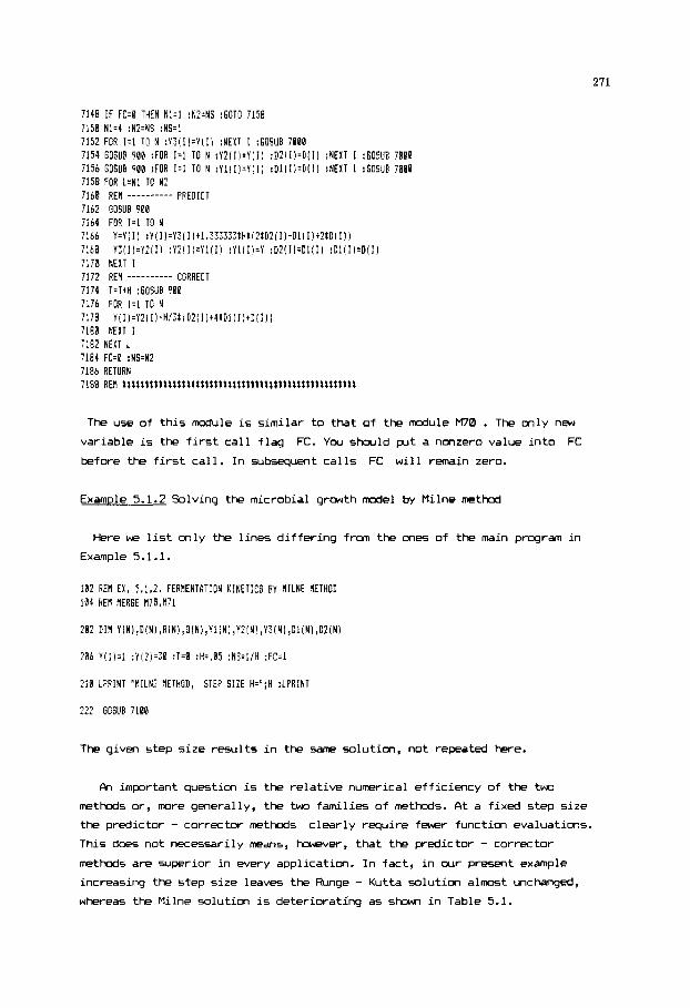
271

7148 IF FC=I THEN N ~ = I :K=NS :GOTO 7158 7150 N1.4 :N?=NS :HS=l 7152 FOR I 4 TO N :Y:!l)=Y(Il :NEXT I :GOSUB 7066 7154 GDSUP 900 :FOR 1.1 TO N :Y2(I)=Y[I) :D?~Il=DIl) :NEXT I :GOSUB 7006 7156 GOSUB 900 :FOR 1.1 TO N : Y l ( l ] = Y ( l ) :Dlill=D(Il :NEXT I :GOSUP 7000 7158 FOR L=Nl TC N? 7 1 b l 7162 1164 7166 7168 7178 7172 7174 7176

7180 7178

RER ---------- PREDICT 50SUB 900 FOR 1.1 TO N Y=Y(I) :Yill=Y31 I)tl.333332;tHti?tD?(I1-DlIIlt2tD(I)) Y3(I)=Y2[I l :Y~lIl=Ylll~ :Vl(I)=Y :D2lIl=Dl(I) :DllI)=Dll) NEXT I RE1 ---------- CORRECT T=T+H :GOSUB 900 FOR 1.1 TO W

NEYT I Y (I)=Y?( I )+H13tiD2( I 1+4tD1(I)tD[II 1

The use of this module is similar to that of the module Ml0 . The only new variable is the first call flag FC. V w should put a nonzero value into FC

before the first call. In subseciuent calls FC will remain zero.

Example 5.1.2 Solving the microbial growth model by Milne method

Here we list only the lines differing from the ones of the main program in

Example 5.1.1.

102 RE! EX. 5.1.2. FERMENTATION KINETICS BY RILNE NETHOD 111 RE! MERGE KO,K71

282 Dlfl Y~Nl,li~N~,RlN1,O~Nl,~liN~,Y?~N),Y3(Nl,Dl~Nl,D2(Nl

206 Ylll=l :Y12)=50 :T=0 :H=.%5 :NS=l/H :FC=I

:lI LPHINT 'MnILNE NETHOD,

222 G O W E 7100

STEP SIZE H=";H :LPRINl

The given step size results in the same solution, not repeated here.

Fh important question is the relative numerical efficiency of the two

methods or, m r e generally, the two families of methods. At a fixed step size

the predictor - corrector methbds

This does not necessarily means, k v e r , that the predictor - corrector methods are superior in every application. In fact, in cur pr-t example

increasing the step size leaves the Runge - Kutta solution almxt unchanged,

whereas the Milne solution is deteriorating as sholKl in Table 5.1.

clearly require fewr function evaluations.

272

Table 5.1 Substrate (y2, g / l ) cmplted a t d i f ferent step s i z e s H ( i n hours)

T i m , h Runge - Kutta Milne

H = 0.1 H = 0.2 H = 0.25 H = 0.1 H = 0.2 H = 0.25

4 1 2 . w 12 .04 12.060 1 2 . w 12.060 1 2 . w 7 4.585 4.585 4.585 4.585 4.585 4.585 8 0.252 0.253 0.257 0.252 0.253 0.242 9 0.wD3 0.003 0.W 0.003 0.m 0.018

10 0.002 0.020 0.002 0.002 -0.m1 -0.022

Experience shows that the re la t ive ly slow Runge - Kutta procedure i s qui te

robust and hence i t i s a g m d choice fo r a f i r s t t ry .

5.1.3 Adaptive step size control

To control the step size adaptively we need an estimate of the local

truncation error. With the Runge - Kutta methods a good idea i s t o take each

step twice, using formulas of d i f ferent order, and judge the error f rom the

deviation between the two predictions. Selecting the coeff ic ients i n (5 .m)

t o give the same aij and di values i n the two formulas a t least f o r some of

the internal function evaluations reduces the overhead i n calculation. For

example, 6 function evaluations are required wi th an appropriate pair of

fourth-order and f i f th-order formulas ( re f . 5) .

I n the predictor - corrector methods the magnitude o f the f i r s t correction

i s an imnediate error estimate with no additional cost.

From the actual step size ha,-, error estimate ESt and the desired error

bound Edes a new step size hn, can be selected according t o

(5.28)

where p i s the order of the method. The expcnent p instead of (p+l ) i n

(5.28) resul ts i n a more conservative step size control, taking i n t o account

also the propagation of errors.

The mst sophisticated d i f f e ren t i a l equation solver considered i n this took

and discussed i n the next section includes such step size control. I n contrast

t o m o s t integrators, bowever, i t takes a fu l l back step when facing a sudden

increase of the local error. I f the back step i s not feasible, f o r example a t

s tar t , then only the current step i s repeated with the new step size.

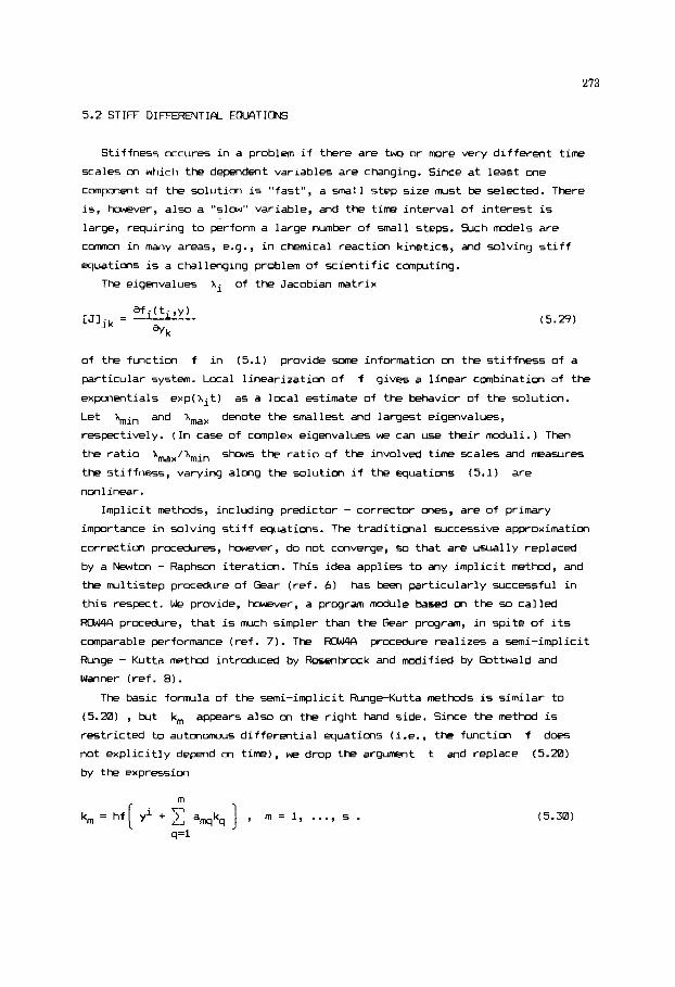
273

5.2 STIFF DIFFERENTIFIL EWTIONS

Stiffness occures in a problem if there are two or m r e very different time

scales on which the dependent variables are changing. Since at least one

cwnponmt of the solution is "fast", a small step size must be selected. There

is, hOwever, also a "slow" variable, and the time interval of interest is

large, requiring to p&form a large number of small steps. Such models are

c m in many areas, e . g . , in chical reaction kinetics, and solving stiff

equations is a challenging problem of scientific canplting.

The eigenvalues Xi of the Jacobian matrix

of the function f in (5.1) provide s m information on the stiffness of a

particular system. Local linearization of f gives a linear combination of the

expcnentials exp(xit)

Let Xmin and xmax denote the smallest and largest eigenvalues,

respectively. (In case of canplex eigenvalues we can use their moduli.) Then

the ratio

the stiffness, varying along the solution if the equations (5.1) are

non 1 inear.

as a local estimate of the behavior of the solution.

hmax/Xmin shows the ratio of the involved time scales and n-easures

Implicit methods, including predictor - corrector ones, are of primary

importance in solving stiff equations. The traditional successive approximation

correction procedures, however, do not converge, so that are usually replaced

by a Newton - Raphsan iteration. This idea applies to any implicit method, and

the rrultistep procedure of Gear (ref. 6) has been particularly successful in

this respect. We provide, however, a program mcdule based on the so called

procedure, that is rruch simpler than the Gear program, in spite of its

camparable performance (ref. 7). The RCWW procedure realizes a semi-implicit

Runge - Kutta method introduced by R-brock and modified by Gottwald and

Wanner (ref. 8 ) .

The basic formula of the semi-implicit Runge-Kutta methods is similar to

(5.20) , but km appears also on the right hand side. Since the method is

restricted to auton-s differential equations ( i . e . , the function f does

not explicitly depend on time), we drop the argument t and replace (5.20)

by the expression

(5.30)

274

We need to solve s sets of nonlinear equations, but Rosenbrock devised a

much simpler procedure. L inear izat im of the m-th set of equations i n (5.30)

around the point

m-1 ’ - ? - I

y = y1 + L, aqkq

q=l

gives the equations

(5.31)

(5.32)

fo r k,, where I denotes the n m iden t i t y m a t r i x , and n i 5 the number of

dependent variables (the dimension of the y vector). Furthermore, the

Jacobian m a t r i x J i s evaluated only a t the beginning o f the current time

interval, and the a, c o e f f i c i m t s are ident ical f o r any m. The

fourth - order method then requires the solution of 4 sets o f l inear

equations

Ek, = r, , m = 1, 2, 3, 4 (5.33)

where

Since a l l 4 sets of equatims i n (5.33) have the same coeff ic ient matrix E,

a single LU decomposition i s su f f i c i en t as described i n Sections 1.3.2 and

1.3.3. The next point of the solution i s predicted by

yi+l = yi + blkl + b2k2 + b3k3 + b4k4 (5.34)

whereas

Ei+l = e l k l + 4 k 2 + e ~ k 3 + e4k4 (5.35)

i s an estimate of the local error vector. The values of the coeff ic ients

involved can be found i n the l i n e 7260 through 7272 of the following program

module.

275

Prosram module M / 2

7208 REN t t t l t t t t t t t t t t t t ~ t t t t t t t ~ l t t t t t k t t t t ~ ~ ~ t t l ~ t t t l l ~ l k 7282 REM t SOLUTION OF STIFF DIFFERENTIAL EBUATlONS I 7204 REM t SEMI IMPLICIT-RUNGE KUTTA METHOD WITH BICKSTEPS t 7206 REH t ROSENBROCK-GOTTWALD-WANNER t 7283 REH t t t t t t t t t t t t ~ t t t ~ t t t t ~ t t t i t t t t t i ~ t t t r t i t ~ i t t i i i t t t i 7218 REH INPUT: 7212 REH N 7214 REH T 7216 REM YIN) 7218 RER TE 7220 REIl EP 7222 REN H

7226 REM OUTPUT: 7228 REM ER 7238 REM 7232 REH 7234 REM T 7236 REM Y(N) 7238 REM H 7240 REM I P 7242 REM IR

7224 RE! I n

NUHRER OF DEPENDENT VARIABLES INITIAL TIME ItlITIAL CONDITIONS REQUIRED END TIME RELATIVE ERROR TOLERANCE INITIAL TIME STEP SIZE MAXIMU! NUMBER OF STEPS

STATUS FLAG 0 SUCCESSFULL SOLUTION I NUMBER OF STEPS INSUFFICIENT

END TIME SOLUTION AT END TIRE SUOOESTED SIZE OF NEXT STEP NUMBER OF ACCEPTED STEPS NUMBER OF REPEATED AND BACKWARD STEPS

7244 REM USER SUPPLIED SUBROUTINE: ?246 REH FROM LINE 988: T,Y(N) --) O ( N ) ( RHS EVALUATION 7248 RE1 AUXILIARY ARRAYS: 7258 REM E(N,NI,A(N,N),RIN),YO(N),YLlN)

7254 REM MODULES CALLED: H14,M15 7256 IF T?=TE THEN ER.8 :GOT0 7414 7258 RElr ---------- INITIALIZATION 7260 Rl=.438 :A2=.9389487 :83=7.387954E-82 7262 C1=-1.943474 :C2=.4169575 :C3:1.323968 7264 C4=1.519513 :C5=1.353788 :C6=-.8541515 7266 81=.7298448 : B2=5,418698E-B2 7268 B3=.2815994 :B4=.25 7270 E1=-1.908589E-82 :E2=.2556888 1272 ES=-B.b38163E-02 :E4=.25 7274 IP.0 : I R 4 :LS=-l :LE4 :SF4 :TR=T 7276 FOR I=l TO N :YOlI)=Y(I) :NEXT I 7278 REM ---------- MAX NUMBER OF STEPS OR END TIME REACHED 7288 IF IP)=lM THEN ER=I :GOT0 7414 7282 IF TtH?=TE THEN LEE-1 :HO=H :H=TE-T

JACOBIRN HRTRIX 7284 RE)I _ _ _ _ _ _ _ _ _ _ 7286 GOSUB 908 7288 FOR 1.1 TO N :R(I)=D(I) :NEXT 1 7298 FOR J.1 TO N 7292 Y=Y ( J ) :D=ABS(Y )t.8$ltlE-15 :Y(J)=Y+D 7294 GOSUB 9BB 7296 FOR 1.1 TO N :E(I,J)=(D(I)-R(II)/D :NEXT I 7298 Y(J1.Y 7318 NEXT J 7302 REN _ _ _ _ _ _ _ _ _ _ LU DECOtiPOSITlON 7384 FOR 1.1 TO N :FOR J=l TO I4 7306 A ( I, J I=-, 3951HtE 1 I, J )- ( I d 1 7388 NEXT J :NEXT I 7318 6OSUB 1481 7312 IF ER THEM H=H/2 :GOT0 7384

7252 REM R1 IN) ,R2(N) ,R3(N) ,R4(N) 5 X IN)

276

ONPUTE STEP RE\ _ _ _ _ _ _ _ _ _ _ C 7316 FOR 1.1 TO N :W(I):HtR(I) :NEXT I 7% GOSUP 1501 7 3 3 FOR I=l TO N 7322 R1( I )=XI I ) :Y(I)=YO( I )tAltX( I) 7324 NEXT 1 7226 GOSUP 901 7:28 FOR 1.1 TO N :X(I!~HtD!I)tCltPl(I) :NEXT I 7330 G W B 1500 7332 FOR I=l TO N X 4 R2( I )=X!I) :YiI)=YO!I ItG2tR1( I )tR31R2( I) 7335 NEXT I 7738 GOSUE 900 7349 FOR 1.1 TD N :X(!)~HII)(I)tC~tR1!!ItC~tRZ!I) :NEXT I 7542 GOSUR 1500 !!44 FOR I=: TO N 7346 K(I!=X!Ij :K(I)=HtD( I)tC4tRl(I)+CSIR~iI!+C~lR3(1) 734a NEXT I 7351 GCSUB 1501 7352 FOR 1=1 TO N -7 i .,54 84 ( 1 ! = X ( I ) : Y ( I ) = Y O ! I )+PI tP1 ( I )+P?tU( I )tB3tR3( I )tP4iR4! I! 7356 NEXT I 7358 T=!+H T I h @ REH ---------- ESTIMATE ERROR ?:52 ES=EP,'lt Y 6 4 FOB 1.1 TO N !:At, S!.BBS(E!tRl(I)tE?tRS( I)tE3tR3( I )+E4tR4( I!! ?368 S:=AESiY(Ij) :S?:kES(YO(I)) X70 S=:tS!!(S?tS3tEPIlElB) Y!? IF S'ES THEN ES=S Z 7 4 #EXT I 7376 RE!! ---------- NEPl STEP SIZE 7378 S=. 9t i EPIES)' . 2fm !181 HZStSFtH

CHECK ERROR 7 y i _____.____

7184 IF ES"EP THE# 7480 7386 REN ---------- ACCEPT STEP AND INCRERSE STEP FACTOR SF 7388 IP=IPtl 739 I F LE THEN H=HO :ER=B :6@T@ 7411 3 9 2 FOR 1.1 TO N :VL(I)=YO(I) :YO(I)=YiI) :NEU I 7594 TL=TR :TR=T 7396 LS.0 :SF=I.$!ISF :IF SF!! THEN SF.1 7398 GOT0 7281 7410 lB=lR+l :LE=C: IF NOT LS THEN 7409 7402 RE8 ---------- REPEB! CURRENT STEP IF BACKSTEP IS NOT POSSIBLE 7484 FOB 1=1 TO N :V(I)=YO(I) :NEXT I 7415 T=TE :GOT0 !304 !408 REV ---------- STEP P R C I PNL HODERATE STEP FACTOK SF 7411 FOR I=l TO N :Y(I)=YL(I) :YO!I)=K(I) :NEXT I !412 IP=IP-I :T=TL : T k T : LS=-1: SF:.PtSF :6OTO 7285 7414 BETURN 741b RE8 l t ~ ~ t l t t t t t t l t t t t t t t t t t t t t t t ~ t t ~ t ~ ~ ~ t t l t t t ~ 4 ~ ~ t 4 t ~ 4 t ~

4 '

In contrast to the modules M70 and M71 , here we s p e c i f y the end t i m e TE

i n s t e a d of the number of steps, s i n c e t h e i n i t i a l s t e p s i z e H is a d a p t i v e l y

decreased or inc reased i n o r d e r to keep the r e l a t i v e error j u s t below the

th re sho ld EP . The suggested v a l u e s of the t h re sho ld are between 0.01

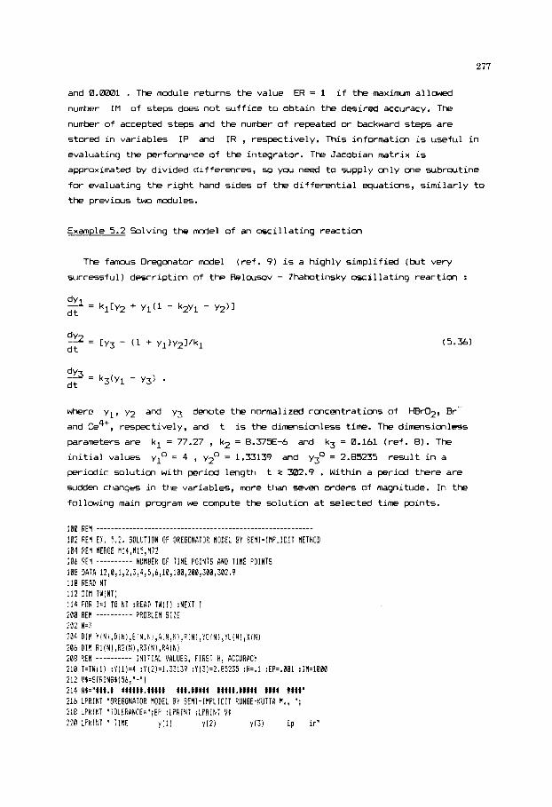
277

and 0.W1 . The module returns the value ER = 1 if the maxin-um allowed

number I M of steps does not suffice to obtain the desired accuracy. The

number of accepted steps and the number of repeated or backward steps are

stored in variables IP and IR , respectively. This information is useful in evaluating the performance of the integrator. The Jacobian matrix is

approximated by divided differences, so you need to supply only one subroutine

for evaluating the right hand sides of the differential equations, similarly to

the previous two modules.

Example 5.2 Solving the model of an oscillating reaction

The famous Oregonator model (ref. 9) is a highly simplified (but very

successful) description of the Belousov - Zhabotinsky oscillating reaction :

where yl, yz and y3 denote the normalized concentrations of I-BrO2, Br-

and Ce4+, respectively, and

parameters are kl = 77.27 , k2 = 8.375E-6 and k3 = 0.161 (ref. 8). The

initial values yl0 = 4 , yZD = 1.33139 and yJ0 = 2.85235 result in a

periodic solution with period length t % 302.9 . Within a period there are sudden changes in the variables, m r e than seven orders of magnitude. In the

following main program we cmplte the solution at selected time pints.

t is the dimensionless time. The dimensionless

105 RE\ ________________________________________------------------- l@? RE\ E l . 5.2. SOLUTION OF OREGONATOR MODEL BY S E M I - I I I P L I C I T NETHOD in4 PEN MERGE M!4,MlS,H7? LQb 9EN ---------- NUMBER OF T I N E POINTS AND TINE POINTS 108 DATP 12,%~1,?,!,4~5,6,10,100,?08~.~~0,~0?,9 110 HERD NT 112 0114 TY(NT1 114 i0H 1.1 TO NT :READ Ti4[I) :NEXT I 3 0 REM ---------- PROBLEM S I T E :a2 N.3 204 DIN Y I N 1 B i N ! ! E I N. I! ! B i N , I! 1 , P I N i ! Y O 1 N 1 I YL i N ! X I N ! 206 DIY R I I N ) ,R;I#! ,R3(N! , l i 4 i N i 288 9EM ---------- I N I T I A L '!!ALUES, FIRST H, ACCURACY 110 T=TW!l) :?!1)=4 :YI2)=1.!'1!9 :Y(3!=?,95?35 :H=.l :EP=.0Bl :IN=100B Y Z V b 4 T F t I N 6 $ ( 5 b , " - " ! 214 AB="XWl,# WWWWW#.11##X W#t.lttt# $ItIW.Wttlt W t fltt' Zlb P R I N T "OfiEGONATOR HODEL BY S E M I - I H P L I C I T RUNGE-KUTTA I . , "; iie LPHINT "TOIERANCE=~:EP :IFHINT :LPRIC; ~t X I LPfiI!!T " YIME y i : i Y I Z ) y ( 3 ! i p ir'

278

222 LPHINT V I 224 LPRINT USING AI;T,Y(l),YIZ),Yl3)

228 FOR 10.2 TO NT 230 TE=TW(ID) :GOSUB 7200 232 LPRINT USING B$;T,Y(l) , Y ( 2 ) ,Y (3 ) , IP,IB 234 NEXT ID 236 LPRINT V I :LPRINT 238 STOP

982 O(lP77.27t (Y (2)tY 11) t (1-8.375E-BblY (1)-Y (2) 1 ) 904 DIZI=(Y(3)-(ltY(I))tY(Z))/77.27 906 D(3)=.lblt(V(l)-Y(3)) 908 RETURN

CALL SOLUTION WOPULE FOR EACH TIHE POINT ?1J REM _ _ _ _ _ _ _ _ _ _ LL

RIGHT HAND SIDE EVILURTION 900 RE! --------__

I n addition t o the so lut im, the number o f accepted steps ( i p ) and the number

of back steps or repeated steps ( i r) are also printed t o show how the step

size c m t r o l works.

OREGONBTOR MODEL BY SEMI-IRPLICIT RUNGE-KUTTR H . , TOLERRNCE- ,001

TIflE

Q.0 1.0 2.0 3.6 4.0 5.0 6 . 8

10.0 100. 8 280.0 300.0 302.9

4.00080 4.52980 5.35444 6,93755 12.43387

97271.55000 1.00214 1.08368 1.85098 3.13234 4.01773

116764 .e~m

.- _------- ____.

1.33139 I . 28090 1.22638 1,16312 1.17232 0.82421 0.18801

785.15818 273.45220 20.54734 1.46751 1.32940

. --_ - - -_ - - - .

y(3)

2.85?$5 3.66899 3.33716 3.74294 4,52226

2839.26000 18304.12000 21 132. 22000

1.01394 1.84376 2.44688 2.85972

-------

. _ _ _ _ _ _ _ - _-_

ip i r

5 0 4 0 4 0 6 1 58 5 16 0

183 3 224 0 31 2 30 1

b 0 _-- -----

Exercise

0 T r y t o solve the Oregmator model using a n m - s t i f f integrator as the

module M70 . Commnt M the step size needed f o r a reaMnable accuracy.

5.3 SENSITIVITY INKYSIS

I n t h i s s t i m we consider the parametrized vector d i f f e ren t i a l equation

(5.37)

where p denotes the np-vector o f parameters. The vector of sens i t iv i ty

279

coefficients to the parameter pj is defined by

(5.38)

These partial derivatives provide a lot of information (ref. 10). T k y show

how parameter perturbations ( e . g . , uncertainties in parameter values) affect

the solution. Identifying the unimportant parameters the analysis may help to

simplify the model. Sensitivities are also needed by efficient parameter

estimation praedures of the Gauss - Newton type. Since the solution y(t,p)

is rarely available in analytic form, calculation of the coefficients sj(t,p)

is not easy. The simplest method is to perturb the parameter

differential equation with the modified parameter set and estimate the partial

derivatives by divided differences. This "brute force" approach is not only

time consuming (i.e., one has to solve np+l sets of ny differential

equations), but may be rather unreliable due to the roundoff errors. A much

better approach is solving the smsitivity equations

pj , solve the

where the i,j-th element of the Jacobian is given by

(5.39)

(5.40)

The sensitivity equations (5.39) are derived by differentiating (5.37)

with respect to

hand side. The initial values to (5.39) are given by

pj , and changing the order of differentiation on the left

(5.41)

The sensitivity equations (5.39) can be solved simultanmusly with the

original equations (5.37). Althwgh the special structure of this extended

system of differential equations enables m e to devise more efficient special

methods (see, for example, refs. 11-13), in the following example we solve the

equations using the general purpose integrator module M72 . The straightforward method not making use of the special structure of the sensitivity equations is

called direct method of sensitivity analysis.

Example 5.3 Parameter sensitivities in the microbial growth model

In order to discuss the practical identifiability of the model studied in

Examples 5.1.1 and 5.1.2, Holmberg (ref. 3) computed the sensitivities of the

microorganism concentrations y1 and substrate concentration y2 with

280

respect to the parameters V,, K,, Kd and Y. To repeat the computations, we

need the part ia l d e r i v a t i v e s

(5.42)

and

The i n i t i a l va lues are

i n i t i a l va lues o f the concentrat ions y1 and y2 do not depend upon the

parameters i n v e s t i g a t e d . ) To solve the extended system of d i f f e r e n t i a l

equations t h e fo l lowing main program is used:

sj(O,pl = 0 , j = 1, 2, 3 and 4 . (Note t h a t the

281

900 REK _ _ _ _ _ _ _ _ _ _ RIF T JH. H A M SIDE EVALUATIOM 90: M0=KStY(?) :Nl=Y(?)lN0 :M2=Nl/H0 :M3=KS/M0/b0 904 N4=VMiHl-K3 :15=VNttt3iY!l) :M6=-\'M/YYtNl :M74M/VVtW3tY(lj 906 RE! - ORIGINRL EQUATIONS 908 Ctli \'YtRltY!1l-KDtY!lj 9:0 D(2) =-VtlIYYLNlti'(l! 912 REH - SENSITIVITY EQUilTIOMS WITH RESPECT TO Vfl 914 Gi3) = NltV(1) tM4tV(3)tHSiY (4) 916 D ( 4 1 =-VNlYY M l t Y (1 j tH6tY ( 3 ) tM7tV (4) 918 REM - SENSI1I'~ITY EQUOTIONS WITH RESPECT TO Ks 928 D( 5) 4Ntti2tY (1 1 tW4tY 15)ttlStY (6) 922 D(6) = VN/YYtM2tY(1) tH6tYIS)+H7tY(6) 924 RE! - SENSITIVITY EOUATIONS WITH RESPECT TO Kd 926 D(7) =-Y(l) tI4tY (7)+\5iY (8 ) 28 Dl81 = M6tY (7)+M7tV(8) 930 REP! - SENSITiVITY EQUATIONS WITH RESPECT TO Y 932 D(9) = tN4iY(9)tRSiY(18)

936 RETURN 934 DI in)= v n i Y Y / v Y i w ! 1) t n b t ~ (9)tn7ty I 10)

Instead of the sensitivities sj(t,p) , in most applications we use the vectors of semi-logarithmic or normalized sensitivities, defined by

*/'log Pj = ~jh//aPj - (5.44)

The last four colurms of the following output list the matrix semi-logarithmic sensitivities consisting of n y m t = 22 rows and np = 4

columns. This matrix is called normalized sensitivity matrix.

S of

SEMI - LDGRRITHNIC IdYiidlogPj) SENSITIVITY NATRIW

TI\E,h CO#CE#THilTi@N PARRNETER SENSITIVITY g / l VP Ks Kd Y

___-___-________________________________---------------- 0.0 yl 1.001 0,000 0.090 8.0B0 0.000

y 2 30.000 0,080 8,000 0.000 0.000 1.0 yl 1.498 0.679 -0.063 -8.875 0.001

y2 29.068 -0.691 B.107 8.025 8.931 2.0 yl

Y2 3.0 yl

Y:

Y ? 5.6 yl

Y2 6.0 yl

Y2 7.0 yl

Y2 8.0 yl

y? 9.0 yl

Y ? 10.0 y l

Y2

4.0 )1

2 , ;:o :!,678 3.339 25,616 4.955

22.581 7.290 18.185 10.524 12.060 14.385 4.586 16.20; 0.252 15.557 e ,003 14.880 0.008

. - _-------

2,023 -1 743

4.496 -5.675 e I798

-11.871 15.770

-27 I &. 209 25.b72 -37.461 31.820 -46.466

8 . 8 i 2 -7.873 4.036 -0.123

3.771 -0.002

'.*

--

-0.190 -8.224 0.007 0.328 0.131 2.318 -0.431 -0.499 0.029 8.756 0.389 4.335 -0.872 -8.982 8.101 1.543 8.913 7.245 -i.b45 -1.782 8.333 2.933 1.854 11.237 -2.906 -2.971 1.156 5.211 3.295 15.936 -4.093 -4.810 4.864 7.499 4.289 17.020 -0.544 -2.511 15.644 1.812 8.769 2.525 0.587 -2.728 16.462 8.040 0.013 0.035 8.505 -1.328 15.681 0.001 0.000 0.001

282

kcording to (5.44) the semi-logarithmic sensitivity coefficients show the

local change in the solutions when the given parameter is perturbed by unity on

the logarithmic scale and are invariant under the scaling of the parameters.

0 2 4 6 10 T L m e , h

Fig. 5.3. Semi-logarithmic sensitivity of the substrate with respect to the

parameters Vm, Ks, Kd and Y

Fk sem f r m Fig. 5.3, the substrate concentration is m t sensitive to the

parameters around t = 7 hours. It is therefore advantageous to select more

observation pints in this region when designing identification experiments

(see Section 3.10.2). The sensitivity functions, especially with respect to

and

of the columns in the Jacobian matrix may lead to ill-conditioned parameter

estimatim problem. Principal cwnpcnmt analysis of the matrix

powerful help in uncovering such parameter dependences. The approach will be

discussed in Section 5.8.1.

K, Kd, seem to be proportional to each other, and the near-linear dependence

STS is a

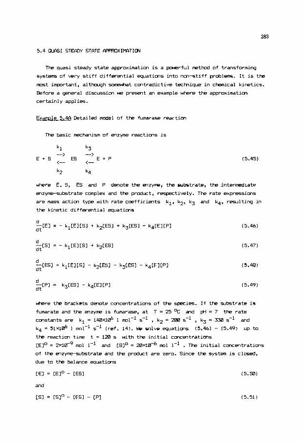
283

5.4 CXlAsI STERDY STATE PPPROXIMFITION

The quasi steady state approximation i s a powerful method of transforming

systems of very s t i f f d i f ferent ia l equations i n t o non-st i f f problems. It i s the

most important, although somewhat contradictive technique i n chemical kinetics.

Before a gmeral discussion we present an example where the approximation

certainly applies.

Example 5.4A Detailed model o f the fumarase reaction

The basic mechanism of enzyme reactions i s

k l k3 -> -->

E + S ES E + P <-- <- k2 k4

(5.45)

where E, S, ES and P denote the enzyme, the substrate, the intermediate

enzyme-substrate cmplex and the product, respectively. The rate expressions

are mass action type with ra te coefficients kl, k2, k3 and k4, resul t ing i n

the kinetic d i f ferent ia l equations

d

d t --[Sl = - klCElCS1 + k2CESl (5.47)

d

d t --[PI = k3CESl - k4CEICPI (5.49)

where the brackets denote concentrations of the species. I f the substrate i s

fumarate and the enzyme i s fumarase, a t T = 25 % and pH = 7 the rate

constants are

k4 = 5 1 d 1 ml-' 5-I ( re f . 14) . We solve equations

the reaction t i m e t = 120 s with the i n i t i a l concentrations

[Elo = ZX~IZI-~ ml 1-l

of the mzyme-substrate and the product are zero. Since the system i s closed,

due to the balance equations

kl = 140Xl& 1 ml-I s-' , k2 = i00 s-' , k3 = 330 5-l and

(5.46) - (5.49) up t o

and [SIo = 20x10-6 ml 1-l . The i n i t i a l concentrations

[ E l = [El0 - CESI (5.3a)

and

CSI = CSlo - CESI - [P I (5.51)

284

it is sufficient to consider the two linearly independent differential

equations

d --[ESl = kl(CE1° - CESl)(CSIo - CESl - [PI) - (k2 + k3)CESl + dt

and + kq( [Elo - CESI 1 CPI ( 5 . 5 2 )

d

dt --[PI = k3CESI - kq(CE1° - CES1)CPl . (5.53)

With the initial step size H = 0.1 s and threshold EP = 0.Wl01, the d u l e

M72 gives the following results:

ENZYilE CGTALYSIS - DETBILEO MECHAIilSM

a,0 h a @

i 2 . 0 l8.@ 24.0 X.9 3 . c 42.8 48.C 54.0 61.E h6.P

*..o !B,8 84.E 5e .e 16.0

182.0 108.0 1 i 4 . 8 12E.0

7?

I .0B00Et01 8.165E-03

0.15EE-08 &.:%3E-e8 0.15YE-08 a.1514E-08 8.1414E-06 0,!4;1E-08 P.1467E-BE( P.1457E-08 0.1451E-06 0.144hE-08 G . 1412E-08 4,1440E-08 B.1438E-08 CS14;’E-08 8.14:bE-OE 0,143SE-08

0.1434E-EB

~ . i b ? 2 ~ - 0 a

0.1435E-08

0.C000Et00 0.3136E-05 41 0.58!2E-05 4 0.8203E-05 : @.;CllE-$4 3 0.1170E-84 3 0.1??2E-04 3 0.1386E-04 3 0.14VE-14 2 0,1509E-84 2 0.154bE-04 2 8.1573E-84 2 0.1593E-04 ! 0,lblbE-84 1 C.lblbE-04 1 0 . lbXE-04 1 0,1527E-04 I 0.lb31E-04 1 0.163E-04 I 0.lb34E-04 1 O.lb3bE-64 1

9

0 0 0 0 0 0 B 0 0 0 0 0 0 0 0 0 0 0 0

The enzyme - substrate complex concentration reaches its maximum value in a

very short time, and decays very slowly afterwards. To explain this special

behavior of the concentration [ES], write its kinetic equation in the form

dCESl/dt = rp - rc , where rp and rc denote the total production and

consumption rates of the enzyme - substrate, respectively. Since rp and rc

are very large, any deviation yields a quick change in

Thus rp = rc . Therefore, it is a gwd

approximation to assume that r = rc at every instant of time, i.e., to find

CESISS for which the right hand side of (5.52) is zero :

rp - rc f 0

[ES] quickly reaches its value where [ESl.

P

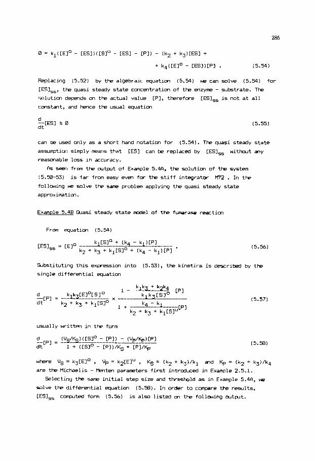
285

0 = kl([Elo - CES])([SIo - [ESI - [PI) - (k2 + k3)CESl +

+ kq(CE1° - CES1)CPI . (5.54)

Replacing (5.52) by the algebraic equation "5.54) we can solve (5 .54) f o r

CESISS, the quasi steady s ta te concentration o f the enzyme - substrate. The

solut ion depends cm the actual value [PI, therefore [ES],, i s not a t a l l

constant, and hence the usual equation

d

d t --[ESl 5 0 (5.55)

can be used only as a short hand notat ion f o r

assumption simply means that [ES] can be replaced by [ES],, w i t h o u t any

reascnable loss i n accuracy.

(5.54). The quasi steady s ta te

As seen f rom the wtput o f Example 5.46, the solut ion o f the system

(5.W-53) i s f a r fran easy even fo r the s t i f f integrator M72 . In the

following w e solve the same problem applying the quasi steady s ta te

approximation.

Example 5.4B m a s i steady s ta te model o f the fumarase reaction

From equation (5.54)

Substi tut ing this expression i n t o

s ingle d i f f e ren t i a l equation

(5.531, the k ine t ics i s described by the

d --[PI = d t

k k [EI°CS10

k2 + k3 + kl [Slo X

usually w r i t t e n i n the form

(5.57)

(5.581

where Vs = k3[EIo , Vp = k2[El0 , Ks = (k2 + k3 ) / k l and Kp = (k2 + k3)/k4

are the Michaelis - Menten parameters f i r s t introduced i n Example 2.5.1.

Selecting the -me i n i t i a l step s ize and threshold as i n Example 5.46, we

(5.58). In order t o compare the r e ~ ~ l t 5 , solve the d i f f e ren t i a l equation

[ES],, computed form (5.56) i s also l i s t e d on the fol lowing wtput.

286

0,E 6.0

17.8 :9.0 :4.8

56.0 47.0 48.0 54.0 60.0 66.0 iL.O

78.0 84.8 90.1 Sb .0

l8?.0 188.0 114.8 120.8

30,a

-r/

8.lb82E-08 8.1553E-88 0.1672E-08 0.1592E-08 8.1563E-08 0. 1S37E-08 0.1514E-08 R.1494E-08 8.1479E-88 0.1467E-BE 0.1457E-88 0.1451E-08 0.1446E-08 0.1442E-08 0.1440E-08 0.1438E-08 0.1K7E-08 0.1436E-88

0.143E-08 0.1434E-88

0 . 1 4 3 5 ~ 4 a

0.0000Et'M 0.3136E-85 0.5873E-85 0.8204E-05 8.1014E-04 B.1170E-04 0.1292E-14 0.138bE-04 0.1457E-04 0.1509E-04 0.1546E-04 8.1573E-84 0.1593E-04 0.1606E-04 R.lbl6E-04 l.lb?!E-04 B.lb27E-04 0.1631E-04 0.1633E-04 0.1655E-04 0.1636E-04

9 2 2 2 I 1 1 1 1 1 1 1 1 1 1 1 1 1 1 1

3 B 8 0 8 0 0 0 0 0 0 0 0 8 0 0 0 0 0 B

As seen from the output, the number of steps required is significantly reduced.

Nevertheless, apart fran a very short induction period, the solution

essentially agrees with that of the detailed model.

Exercise

o Solve Example 5.4B using the program module M70 . Try to solve Example 5.4A with the same method. Comnent on the differences in accuracy, required step

size, etc.

5.5 ESTIMATIDN CF PNWETERS IN DIFFEREMIN- ECXlATIaVS

In this section we deal with estimating the parameters p in the dynamical

model of the form ( 5 . 3 7 ) . As we noticed, methods of Chapter 3 directly apply

to this problem only if the solution of the differential equation is available

in analytical form. Otherwise one can follow the same algorithms, but solving

differential equations nwrically whenever the computed responses are needed.

The partial derivations required by the Gauss - Newton type algorithms can be

obtained by solving the sensitivity equations. While this indirst method is

very general (ref. 151, it is so time consuming that m y be not feasible on a

personal compter.

The direct integral approach to parameter estimation we will discuss here

applies only with all variables yl, yZ, ..., yny a m r e efficient alternative. Let tl, t2, ..., hm dmote the sample time points with tl = 0 . The unknown parameters p are to be estimated from

the set of observations { (ti,yi) , i = 1, 2, ..., nm } . The basic idea of the direct integral method (refs. 16-17) is transforming the vector

differential equation (5.37) into the equivalent integral equation

observed, but then it offers

I

( 5 . 5 9 )

and approximating the integrand by cubic spline functions that interpolate the

points { (ti,f(;i,p)) , i = I, 2, ..., nm } . Evaluating the integrals at the current estimate of the parameters cmverts the problem into an algebraic

m e which can be solved by the nwlinear least squares algorithm of Section

3.3.

p

f

P Let S (t) denote the ny-vector of natural cubic splines interpolating the

values { (ti,f(;i,p)) , i = 1, 2, ..., nm } . Introducing ti-e veztor

t) dt

of nmmy el-ts we can write the objective function of the direct integral

mthod in the usual form (3 .39 ) .

The Jacobian matrix defined in (3.41) can be easily computed by the same

interpolation technique. The idea is to differentiate ( 3 . a ) with respect to

the parameters changing the order of differentiation and spline integration.

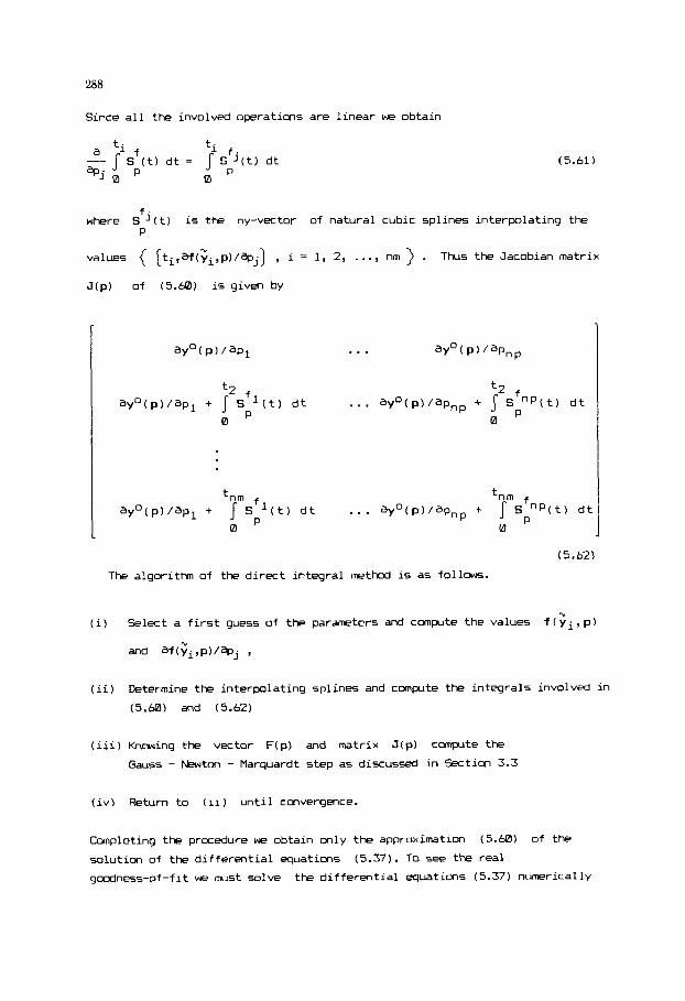
288

Since all the involved operations are linear we obtain

t. a ti f f.

+ j m P 0

--- S (t) dt = S '(t) dt P

(5.61)

f.

P where S '(t) is the ny-vector of natural cubic splines interpolating the

values { (ti,af(yi,p)/Wj) , i = 1, 2, . . . , nm } . J(p) of ( 5 . 6 0 ) is given by

I

Thus the Jacobian matrix

...

(5.62)

The algorithm of the direct integral method is as follows.

-L

(i) Select a first guess of the parameters and cmpute the values

and af(;i,p)/+j 9

f(yi,p)

(ii) Determine the interpolating splines and compute the integrals involved in

(5.60) and (5.62)

(iii) Knming the vector F(p) and matrix J(p) cmplte the

Gauss - W t o n - Marquardt step as discussed in Section 3.3

(iv) Return to (ii) until convergmce.

Completing the praedure we obtain only the approximation

snluticn of the differential equations

goodness-of-fit we must solve the differential equations (5.37) numerically

(5.60) of the

(5.37). To see the real

289

with the parameter estimates ^p and initial conditions f (^p) , but only once. Since spline interpolation and integration is mcht faster than solving the

sensitivity equations and the original differential equations, the direct

method is superior to the indirect m e in terms of numerical efficiency,

whenever it is feasible.

In spite of its simplicity the direct integral method has relatively g o d

statistical properties and it m y be even superior to the traditional indirect

approach in ill-conditioned estimation problems (ref. 18). Good performance,

Inever, can be expected m l y if the sampling is sufficiently dense and the

measurement errors are moderate, since otherwise spline interpolation may lead

to severely biased estimates.

The following program d u l e is a dification of the nonlinear least

squares d u l e

equation solution involved it is rather lengthy.

M45. Because of spline interpolation and differential

Proqram module M75

7500 REM t t t t t t t t t t t & t t l l t i t t l t t l l t t t t t t t t t l l t l t t t t t t t t & t & t t 7502 FEM t ESTIMATIOI I OF PARAMETERS I N DIFFEREt iTIAL t '584 REM I EQUATIONS E V DIRECT INTEGRAL HETHOD t ' 5 @ b FEY tElTENSICiN OF THE HIMtfELBLAU-JDNES-5ISCHOFF METHOD& ?5#B PEI l t t t i l t t t t t t t l l t t t t t t t t t t & t t ~ t ~ t t t t t t t t t t t t & t t t t t t t 75:0 FEM !MFUT: 751: RE! NM NUMBER OF SAMPLE POINTS ?:I4 RE!I YY NUIRER OF DEPENDENT VARIABLES 7516 HEM NP NUMGEfi OF PARAMETERS 7518 REM T ( N M ) SIMPLE TIME POINTS 7528 E'EN ViNM,hiY! TAELE OF OBSERVATIONS 7522 RE1 W I I D E N T I F I E R OF WEIEHTING OPTIONS 7524 RE! 0 IDENTICAL WEIGHTS I W I 1 3 1 ! = 1 9 WII ,J !=0 7526 RE! 7528 ?EN 2 USER-SPECIFIED WEIGHTS 7533 REM 7532 RE\ 7 5 3 REM P ( N P i I N I T I A L PARARETER ESTIMATES 7536 REI( EP THRESHOLD DM RELATIVE STEP LENGTH 7538 KEY I N M A ~ I M U M NUMBER OF ITERATIONS 7 5 4 0 HEM CETPUT: 7542 REH ER ST4TUS FLAG 3 4 RE1 I SUXESSFUL ESTIMATION ? 5 4 6 FEt? i REQUICED T?FESHOLD NOT ATTAINED 7545 PEN PiNP! PARMETEK ESTIMATES 7 5 5 0 RE1 ,.... FURTHER RESULTS ARE PRINTED I N THE NODULE '552 FEM USER-SUPPLlEI; SLIBROUTINES: 7554 HEM FROM L:%E SEE: 75% SEN T I 1 !...! ny) AND PI1, ..., np! --i @(lq...,ny) 7 3 8 RE8 I EVALUATE RHS OF @ I F F . EQUATIONS ) 7:CD REM 75b2 REM FRO8 L I N E 808: 7564 RE! Fii, ...! n p i --! YIIl !...! n y ) 7566 REt! I EVALUATES I M T I R L CONDITIONS FOR VRRIABLES I

1 RELATIVE WEIGHTS ( WI I I ) =CONST/V! I, I IA2,W ( I , J )=a 1

GI'JEN BY FURTHER INPUT AS W(tiY,NY) MA!iilI OF WEIGHTING COEFFICIENTS I ONLY FOR U I = ? j

290

7568 RER RUXILIARV ARRAYS: 7570 REH A 1 INP HAX NV] , [NP HA1 NVI ) ,C( NP,NP) ,U(NP,NP) ,BINP ,DE(NP), 61 NV ,NPl 7572 REH FINH) , I INW) ,S(4,NBl ,SF(NH,NY) ,SGINli,NY ,NP) ,YG[NY ,NPl , WINY ,NY 1 7574 REtl EINY ,NV) ,R[NY) ,VOlNV ) , VL I NV ) ,Rl (NV ) ,R2 (NY 1 ,RJ(NV) ,R4 INV) ,XI NV) 7576 REH HODULES CRLLEO: H14,N15,tl16,Ml8,H41,H6~,H7~

SPLINE KNOTS 7588 FOR M=l TO NH :Z(W)=T(i l ) :NEXT H 7582 REH ---------- GENERATE WEIGHTING COEFFICIENTS 7584 I F W!OO THEN 7588 7586 FOR I=1 TO NV :FOR J.1 TO NV :W[I,J)=-(Id) :NEXT J :NEXT I 7588 EI.0 : E S 4 :PH=.01 7590 REH ---------- SUH OF SQUARES AT STARTING POINT 7592 GOSUB 7816 :GOSUB 7772 7594 REH ---------- START OF ITERATION 7596 LPRINT :LPRINT 'STARTING POINT';TABI25);"SUW SO=';F :LPRINT 7598 FOR K.1 TO NP :LPRIHT T~B(25); 'P( ' ;K;'~=';plW) :NEWT K 7688 FOR 11.1 TO 111 7682 FOR I.1 TO NP :U(K,B)=P[K) :NEXT K :FR=F 7684 REH ---------- COHPUTE T'WT AND W l ' V 7686 FOR K=1 TO NP :BlK)=8 :FOR L = l TO I :CIK.L)=8 :NEXT L :NEXT C 7688 GOSUB 7842 7610 FOR H.1 TO NB 7612 7614 GOSUB 7804 7616 FOR K=l TO NP 7618 FOR L=1 TO K 7620 Q4 7 6 2 FOR 1.1 TO NY:FOR J=1 TO NV 7624 7626 NEXT J :NEXT I :C(K,L)=C(K,L)tA 7628 NEXT L 7630 A=8 7632 FOR 1.1 TO NV:FOR J=1 TO NY 7634 7b3b HEIT J :NEXT I :B(K)=BIK)tA 7538 NEXT K 7648 NEXT H 7b42 REH ---------- NDRRRLIZE CROSS PRODUCT HRTRII 7644 TR.8 :FOR 1.1 TO NP :ClI,8)=ClI,I] :TR=TR+ClI,I) :NEXT I 7646 TR=TRIMP/lEUB 7648 FOR 1.1 TO NP 7650 7652 NE!T I 7654 FOR 1=1 TO NP :FOR J=1 TO I 7656 7658 NEXT J :NEXT 1 7668 REW ---------- MAROUARDT'S COHPROHlSE 7bb2 FOR 1.1 TO NP 7bb4 7666 N I , I ) = C I I,I)+PH 7668 NEXT I 7678 REB ---------- RRTRIX INVERSION 7672 ER.0 :N=NP :GOSUB 16E@ :IF EH=1 THEN 7728 7674 REH ---------- COHPUTE STEP 7676 FOR I=l TO NP 7678 7688 NEXT I

7578 REH -__-______

I F W l = l THEN GOSUB 7792

A=A*W I I , J I t6[ I ,L) tGl J ,K) t P ( L ) & P I K!

A=A+lJl I , J l tGl J , l ) t l V ( H , I ) - V l I ) ) t P l K )

IF CII,B)<=TR THEN ClI,B)=l ELSE C(I,8)=SOR(ClI,B])

U I I , J )=E l I , J 1 :C( I , J ) = C l I , J I IC I I ,81 IC( J ,el

FOR J = 1 TO 1-1 :RlI,J)=C(1,J) :NEXT J

D.8 :FOR J.1 TO NP :D=D*AI I , J ) IC (J ,B ) tB [J ) :NEXT J :D(I)=D/C(I,E)

29 1

7682 REH ---------- CHECK SIGN AND REDUCE STEP IF NEEDED 7684 st=e : ~ = i

FOR 1.1 TO NP 7688 IF XItD(I)i=-.95 THEN XI=-.95iDi1) 76?0 SL=SL+DiI)tD( I) 782 NEXT I :SL=SQRiSL)lXI 7694 RE! ---------- NEW ESTIMTES 7696 FOR 1.1 TO NP :P(I)=U(I,0)tiltXItD(I)) :NEXT I 7698 GOSUB 7816 :60SUB 7772 7708 KEN ---------- PRINT ITERATION STEP 7702 FI="t.it'"̂ *" :LPRINT 7704 LFRIHT "IT=";IT;TRH(lB);"PN=": :LPHINT USING F$;PN; 7706 LPRINT TbB(251;"SUM SQ=";F;TAP(50);"SL=";SL :LPRINT 7708 IF F\=FR THEN 7712 7710 FUR K=l TO NP :LPHINT TAB(25);"Pi ' ; ; l l :n)=n;P(K) :NEXT K 7712 RE1 ---------- END OF PRINT 7714 IF SL(=EP THEN EI=0 :GOTO 7728 7716 RE! ---------- HARQUARDT' PARMETER 7718 IF F(=FR THEN 7722 7726 P!=l0tP!i :GOTO 7660 7722 PH=PHil0 :IF PtK.000001 THEN PN=.000001 .'724 NEkT IT 7726 EI.1 7728 IF FRCF THEN FOR I=1 TO NP :P[I)=U(I,Q) :NEXT I 7730 REM ----------- SOLVE DIFFERENTIAL EQUbTIONS 7732 GOSUB 7908 7734 REfl ----------- COMPUTE E X A l T SUfl OF SQUARES 7736 GOSUB 7772 7738 IF=NMtNV-NP :SE=SQR( F!NF) 7740 RE1 ---------- STANDARD ERROR AND CORRELATION tlATRIX OF PARRHETERS 7742 FOR 1.1 TO NP :FOR 1.1 TO I 7744 A ( I,J)=E( I ,J) 7746 NEXT J:NEXT I 7748 N=YP :GOSUP 1600 :IF ER.1 THEN ES=l :60TO 7764 ELSE ES=0 7750 FOR 1.1 TO NP 7752 Bi I )=SOR(F/NF!A( I , I )/C( I ,0)/C( I ,0)) 7755 C(0,Il=SQR(A(I,I)l 7756 NEXT I 7758 FOR I=l TO NP :FOR J=1 TO NP 7760 Ci I, J)=INT(l080td(I,J)!C(0, I)!C(0,J)t.5)/1008 7762 liEXT J:NEXT I

7766 FOR 1.1 TO NP :FOR J=I TO I :t'!II,J)=U(I,J) :NEXT J :NEXT I 7768 N=NP :GOSUB 1808 7778 6 0 3 7920

7774 F=8 7776 FOR H = l TO N! 7778 IF WI=l THEN GOSUB 7792 7780 FOR 111 TO NY :Y(I)=SF(H,I) :NEXT I 7782 FOR 1.1 TO NY :FOR J=l TO NY 7785 7786 NEXT J :NEXT I 7788 NEXT ti 7798 RETUPN

7764 REM ---------- PRINCIPAL CONPONENT ANALYSIS

7772 RER ---------- sun OF SQUARES

F=F+W( I ,J )! ( V ( H , I )-Y (I ) ),'2

292

7792 RE4 ---------- RELATI!'E WEIGHTING 77S4 FOR 1.1 TO N? 7796

7800 NEXT 1 7802 RETURN 7801 RE1 ---------- JACOEI MATRIX AND RESPONSE 7806 FOR 1.1 TO NY :FOR J=1 TO NP 7808 61 I I J)=58!11, I , J )

7812 FW 1:l TO I Y :Y[l)=SF(tl,I! :NEXT I 7814 RETURN 7816 PER ---------- DIRECT INTEGRAL RESPONSES 7818 GOSUB 888 7828 FOR H=l TO NH 7822 FOR J=1 TO NY :Y(J)=V(il ,J) :NEXT J 7524 GOSUB 900 7926 FOR J=! TO N I :SF(M,J!=D(Ji :NEXT J 7528 NEXT 4 7830 FUR J0.1 TO NY 7832 FOR 4.1 TO NM :FlK)=SFIil,J8! :NEXT N 7834 N=NN :EC=0 :GOSUB 6300 7836 FOR H.1 TC Ntl :SF(n,J0)=SI4,#)+YI(JB! :NEXT H 7838 NEXT J0 7840 RETURW 7842 RE! ---------- CIRECT INTEGRAL JACOB! RATRIX - FIRST TlHE POINT 7844 FOR J=l TO NP 7846 7848 7850 7852 NEXT J 7854 EOSUB 818 7856 FOP I=: TO NY :FOR 3.1 TO NP 7858 YG!I, J)=YGII,J)-YI !I I/DE(J) 7850 NEXT J: NEXT I 7552 REH ---------- - INNER TIKE POINT 78t4 FOR H=l TO NN

7868 FOR !=I TO NP 370 !872 7874 7576 NEXT J !8!8 GOSUP 90% 7888 FOR 1.1 TO NY :FUR J = 1 TO NP 3 8 2 SG(t!,I,Ji=GlI! 3 ) - 0 ( I)/DE(J) 7884 NEXT J: NEXT I 2386 NEXT 7855 FOR IP=l TO NY :FOR J0.1 TO NP 7890 FOR N=1 TO Nil :F(R)=SG(W,IB,J0) :NEXT R 7892 N=NN :EC=0 :GOSUB 6380 7894 FOR N.1 70 NH :SG(H,10,J0)~Sl4,~)tYG(I0,Jfi) :NEXT tl 7896 NEXT J0 :NEXT I f i 7308 RETURN 7908 RE# ---------- SOLUTION OF DIFFERENTIRL EQUATIONS 7982 N-NY :IR:lfi0 :H=lT(21-T(l)l/l0

Y=bBS(V(b,I)! :IF Y!1E-15 THEN Y=lE-15 7798 Hi I! I )=l/Y/Y

7810 NEXT J: NEXT I

DE=.0BltABS(P(J) )tlE-10 :PIJ )=P(J !tDE :GOSUB 880

PI J)=P( JI-DE :DE( J)=DE FUR 1.1 TO NY :YE(I,J)=YI(I!/DE :NEXT I

7866 FOR 1.1 TO NY :yii)=vcn,I) :NEXT I

IIE=.10ltkBSlPl J) )+.0000Bl :P( J )=PI J)+DE :GOSUB 9B'd FOR !=I TO NY :G(l,J)=D[I)/DE :NEXT I P( J )=Pi J -DE :DEI J ) =DE

7904 GOS~~P 8ae 79C6 FOR J.1 TO NY :YlJ)=YI[J) :REIT J

293

7959 FOR 16.2 TO NM 7910 T=TiJ6-1) :TE=TiIGl :GOSUB 7280 7912 IF ER THEN LPRINT 'ER=n;ER,"ERROR I N DIFF. EQU. SOLUTION" :STOP 7914 FOR J = l TO NY :SF(IG,J)=Y(J) :NEXT J 7915 NEXT I6 7918 RETURN 7920 REN ---------- PRINT RESULTS 7922 LPRINT :LPHINT 7924 LPRINT TAR(1S);"ESTIIATION OF PARANETERS IN DIFFERENTIAL" 7926 LPRINT TRP(17) ;'EQUATIONS BY DIRECT INTEGRAL METHOD' 7928 LPRINT :LPRINT :LYRINT 7930 LPRINT . NUtlPER OF JEPEN9ENT VARIABLES ....... ';NY 7932 LPRINT . MUMEER OF PRRRMETERS.. ............... ";NP 7934 LPRINT . NUREER OF TIflE POINTS ............... ';NM 7936 LPRINT . OPTION OF WEIGHTING ................. ';WI; 7938 IF M I 4 THEN LPRINT allDENTICAL 7940 IF W1.l THEN LPRINT '(RELATIVE WEIGHTS)' ;942 IF WI=2 THEN LPRINT '(USER DEFINED WE1GHTS)O 7944 F$="#.#llllltA*" ' :LPRINT :LPRINT 7946 LPRINT " PRINCIPAL COHPONENT ANALYSIS OF NORHED CROSS PRODUCT HATRIX" 7948 LPRINT :LPRINT "EIGENVALUE'; 7950 FOR 1.1 TO NP :LPRINT TAB(10tlt51;' Pl";I;*) '; : NEXT I :LPRIWT :LPRINT 7952 FOR 1=1 TO NP 7954 LPRINT U(O,I), 7956 FOR J = l TO NP :LPRINT USING "11.1111 7958 NEXT I 7960 LPRINT :LPRINT 79b2 V$=STRINGI 178, ' -") :Vl$:STRING$ (55, I-" 1 7964 I F EI=l THEN LPRINT " REQUIRED THRESHOLD NOT ATTAINED" :LPRINT :LPRINT 7966 IF ES=l THEN LPRINT " SINGULAR CROSS PRODUCT RATRII' :LPRINT :LPRINT 7968 FOR 1=1 TO MY 7970 LPRINT :IF NY)l THEN LPRINT "RESPONSE FUNCT1ON";I 7972 LPRIFIT Vl$ :LPRINT 'NO',' Y XEAS"," Y COflP',," RESIDUALn :LPRINT V1$ 7974 FOR M=l TO Nfl

7978 NEXT H :LPRINT V11 7980 NEXT I :LPRINT :LPRIHT 7982 LPRINT ' SGW OF SQUARES [VIA SOLUTION OF ODE). ';F 7984 LPRINT . DEGREES OF FREEDOH ................... ";NF 7986 IF WI.0 THEN LPRINT . STRNDARD ERROR ...................... ";SE :988 I F !41)0 THEN LPRlWT . SIGH4 FRCTOR IN THE WEIGHTS ......... ';SE 7990 GOSUB 4180 7902 LPRINT " CRITICRL I-VALUE AT 95 X CONF. LEVEL 7994 LPRINT :LPRINT V$ :LPRINT 'PARAMETER", 7996 IF ES=B THEN LPRINT ' ESTIMATE'," ST. ERR",'LOWER BOUND",*UPPER BOUND', 7998 LPRINT :LPRINT V$ 8008 FOR 1.1 TO NP EB02 LPRINT ' P(";I;') ', :LPRINT USING F$:Pll), 8004 PB=AFS(Pl I ) tP[ I ) ) 8886 8808 LPRINT 8810 NEXT I 8812 LPRINT V$ :LPRINT 8014 IF ES=l THEN 8038 8816 LPRINT 8818 LPRINT 8 0 3 FOR 1.1 TO NP :LPRINT TA8(18tI);Y P(' ; l ; ' ) "; : NEXT I :LPRINT :LPRINT

';U(J,I); :NEXT J :LPRINT

7976 LPRINT M, :LPRINT USIttG F~;V(N,I),SF(#,I),VIII,I)-SF(M,I)

";I

I F E S 4 THEN LPRINT USING F);PB,P(I)-TtPB,PII)tTtPB,

CORRELATION MATRIX OF PARPHETERS:"

294

T h e i n p u t d a t a s t r u c t u r e is very similar to the me i n t h e d u l e M45 . Two

u s e r r o u t i n e s are to be supp l i ed . T h e f i r s t one starts at l i n e 9wz) and

e v a l u a t e s the r i g h t hand s i d e s of the d i f f e r e n t i a l equa t ions . T h e second

r w t i n e , s t a r t i n g a t l i n e 80.3, s e r v e s f a r c m p t i n g the i n i t i a l c o n d i t i o n s a t

the c u r r e n t estimates of the parameters. I f the i n i t i a l estimates are parameter

independent ( w e know them e x a c t l y ) , then t h i s r o u t i n e s imply puts the know,

v a l u e s i n t o t h e v a r i a b l e s YI(l), ..., YI(NY) . The r equ i r ed partial

d e r i v a t i v e s are generated us ing d iv ided d i f f e r e n c e s approximation. In o r d e r to

ease the u s e of the d u l e a very s imple example is considered here.

Example 5.5 F i t t i n g a Michaelis - Menten type k i n e t i c model

Consider t h e s imple model

(5.63)

wi th unknown i n i t i a l cond i t ion

y ( 0 ) = p3 . (5.64)

T h e d a t a listed i n Table 5.2 are the c o n c e n t r a t i o n s of a drug i n plasma and

c ~ n e f r m a test p r o b l m o f the Eo*1Dp statistical program package ( r e f . 19).

Table 5.2 Observed drug concmtration

No Time, min Concentrat ion, g / l

ti

0 23.6 49.1 74.5 80.0

1m.0 125.5 144.3

24.44 19.44 15.56 10.56 9.07 6.85 4.07 1.67

295

To illustrate the robustness of the direct integral program module, we chose

the starting estimates p1 = 1 , p2 = 1 and p3 = 1 , althwgh ~3 = 24.44

obviously is a better starting guess.

100 HEM _______________-________________________------------------- 102 RE1 EX. 5.1; DlAECT IVTEGRAL PARMETER ESTIMATION 104 RiH BERGE ~!l,B15,Mli,~18,#41,M63,~~~,b75

108 RE# Y Y #B NP

1 2 ?EM [ T I M E All@ CONCENTRATION! :1: CATA 0, 24.44

I!E DATb 4?,1, 15.56 i?l DCTA 7 4 . 5 , 10.56 !2 DATA 80.0, 9.07

126 DATA 125.5, 4.V 128 DATA 117.3, 1 . 5 7 23% REM ---------- RidD DATA AND SPECIFY DINENSIONS 202 REAP NY,NB,NP 3 4 MX=WY :IF MXiNP THEN RI(=NP 286 DIM A[MX , Ir? ! ,CiNP ,NP ) , Ui WP,NP) , B l NP) , CEINP! $1 MY ,NP) , N N Y ,MY) 3 8 DIK FiMM! ,ZINM! ,Si4,NUl ,SFIN!l,NY! ,SG[Nfl,NY ,NF! ,YG(NY,NP) 210 B!B EiNY , N Y j ,R!NVl ,VllNYl ,YLlNY 1 ,RliNY) ,R2!NY I ,RJiNY) ,R4INY) , X [ N Y ) 212 PIM T[NM! ,V (NM,NY! 214 FOR 1.1 TC NH ;lb READ Ti ' l ! :FOR J=1 TO NY :READ V ( U , J I :NEXT J 218 NEXT B 220 REH ---------- SET ITERATiOM CONTROL PARABETERS AND CALL nODULE 222 P(11'1 :P(?)=l :F[:)=l 224 EF=.B01 :I#=JB :WI=0 226 GOSUB 7500 228 STOP

106 REM ---------- Dm

1!@ DATA :, a, 3

116 x T a ~ J . L ~ , 19.44

2 4 DATA ie0.0, 6.35

aea REM ---------- INITIAL VALUE EVALUATION SUBROUTINE a02 YIii)=Pi:) 304 RETURN 9b0 REM ---------- RIGHT HAND SIDE EVRLUATION SUBROUTINE 90: D i li=-Pi I ltri l!! (Pi?]+Y (11 ) 904 R E X R I

Before listing the output, recall that the objective function to be

minimized is based M the approximate response ( 5 . 6 0 ) . The minimum of this

function is 1.01W.02, whereas solving the differential equation ( 5 . 6 3 ) at

the final estimate of the parameters gives the value 1.060729. The direct

integral estimares are acceptable m l y if these two values do not significantly

differ, see (ref. 18).

STARTING POINT SUU SO= 68876.19

Pi 1 ) = 1 P i z ) = 1 P( 3 ) = 1

296

11; 1 P R = E , I E - B l

IT: 2 Ptk0.1E-02

IT= ? Pk4. lE-B3

I T = 4 PM=B.IE-M

IT= 5 PM=B.IE-85

!T= 6 PM:B.IE-PIS

sun SR= 7 1 9 . m a

P i 1 )= ,3919189 P ( 2 ) = 2.950189 P I 3 != 25.26825

SUtl SO= 9.465345

P( 1 != .24710?1 PI 2 ) = 4.258754 P i 3 ) = 24.49897

SUM SO: 1.066295

P( 1 ) = ,2452795 P ( 2 )= 5.326014 P I 3 ) = 21.3834

SUH SO= 1.01a621

PI I ) = ,2474369 P ( 2 != 5.573409 P ( 3 I = 24.38938

SUH SO= 1,818682

P( I ) = ,2475825 P I 2 ) = 5.58522 PI 3 ) = 24.39008

SU\ SQ- 1.01Bb02

SL= 2?.3446k

SL= .5924W4

SL= .2507575

SL= .0472762

SL= 2.199665E-83

SL: 2.64@32E-04

ESTIEATIOI i OF PARMETERS I N DIFFERENTIAL EQUATIONS BY DIRECT INTEGRRL NETHOD

NUKBER OF DEPENDENT VARIABLES ,. I ,, , . 1 KURBER OF PAEIII'IETERS.. . . . . . . . . . . . . . , . 3

O P T I O l OF YEIGHTING ................. B ( I D E N T I C A L WEIGHTS) KDHBER OF TME POINTS ..,...I.. . , . . , . a

PRINCIPAL COMPONENT ANALYSIS OF NORHED CROSS PRODUCT n A T i u x

EIGENVALUE P ( I P ( 2 P I 3 !

k321.124 -.491?98 ,141432 .859146 356.7185 .El1155 - . ? 8 4 5 3 .511119 1.76409 ,316741 ,948176 ,825222

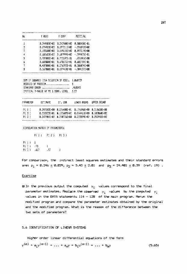
297

SUY OF SQUARES (?'!A SOLZT!ON 3F ODE!. CEEREES OF FREEDOM .................., 5 S T X D 4 R P EREOR , . . , . . . . . , . . . . . . . . . . . . CP!TICCL T-VRL!IE AT 9 5 X C O W . LE'!EL 2 . 5 7

1.068729

.46%593

FARAMETEP ESTIMTE ST. ERR LOWER FOUND UPPER FOUND

P i 1 i 1.247581Et00 0.27640BE-01 B.176546Et00 0.318620EtB0 F( '2 ! 0.5Z5::EtN 0.1336WEt0; 0.864411Et00 0.103060Et02 P i 3 j @.?439@1Et$2 D.3907:6Et00 0 .233E9Et82 0.25394?EtP2

CORRELATION PATRIX 3F PARANETEPf:

For comparison, the indirect least squares est imates and the i r standard errors

are: p1 = 0.246 2 0.029, p2 = 5.43 2 2.01 and p3 = 24.401 2 0.39 (ref. 19) .

Exarcise

In the previous cutplt the complted yi values correspond t o the f i n a l

parameter estimates. Replace the observed yi values by the cmplted y i

values i n the DATA stat-ts 114 - 128 of the main program. Rerun the

modified program and compare the parameter estimates obtained by the or ig inal

and the modified program. What i s the r e a m of the difference between the

two sets of parameters?

5.6 ILENTIFIWTIW OF LINEAR SYSTEMS

Higher order l inear d i f ferent ia l equations of the form

y("') + aly(m-l) + ... + amy = blu(m-l) + ... + bmu (5.65)

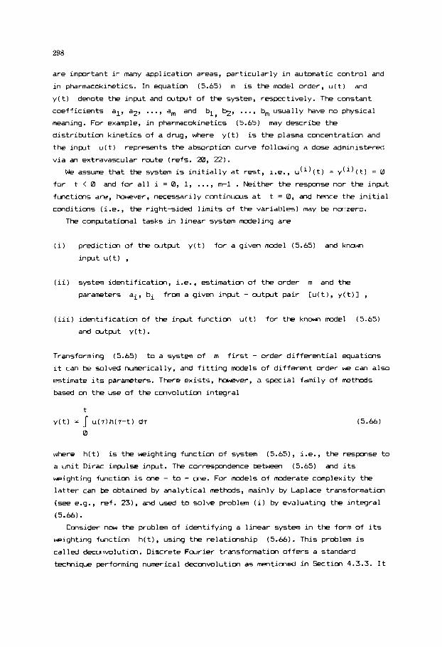
298

are important in many application areas, particularly in autcunatic control and

in pharmacokinetics. In equation (5.65) m is the model order, u(t) and

y(t) denote the input and outplt of the system, respectively. The constant

coefficients al, a2, ..., a, and bl, ba, ..., b, usually have no physical

meaning. For example, in pharmacokinetics (5.65) may describe the

distribution kinetics of a drug, where y(t) is the plasma concentration and

the inplt u(t) represents the absorption curve following a dose administered

via an extravaxular route (refs. 20, 22) .

~e assume that the system is initially at rest, i.e., u(l)(t) = y(i)(t) = 0

for t < 0 and for all i = 0, 1, ..., m-1 . Neither the response nor the input functions are, however, necessarily continuws at t = 0 , and hence the initial

conditions (i.e., the right-sided limits of the variables) may be nonzero.

The computational tasks in linear system modeling are

(i) prediction of the output y(t) for a given model (5.65) and known

input u(t) ,

(ii) system identificatim, i.e., estimation of the order m and the

parameters ai, bi from a given input - output pair [u(t), y(t)l ,

(iii) identification of the input function u(t) for the know model (5.65)

and output y(t).

Transforming (5.651 to a system of m first - order differential equations

it can be solved numerically, and fitting models of different order we can also

estimate its parameters. There exists, however, a special family of methods

based on the use of the convolution integral

(5.66)

where h(t) is the weighting function of system (5.65), i.e., the response to

a unit Dirac impulse inplt. The correspondence between (5.65) and its

weighting function is me - to - one. For models of moderate complexity the

latter can be obtained by analytical methods, mainly by Laplace transformation

(see e.g., ref. 23), and used to solve problem (i) by evaluating the integral

(5.66).

Cu-isider now the problem of identifying a linear system in the form of its

weighting function h(t), using the relationship ( 5 . 6 6 ) . This problem is

called deconvolutim. Discrete Fourier transformtion offers a standard

technique performing numerical deconvolutim as mentioned in Section 4.3.3. It

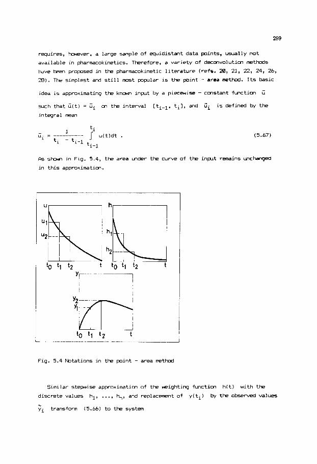
299

requires, however, a large sample of equidistant data points, usually not

available in pharmacokinetics. Therefore, a variety of deconvolution methods

have been proposed in the pharmacokinetic literature (refs. i0, 21, 22, 24, 26,

28). The simplest and still rest popllar is the point - area metkd. Its basic

idea is approximating the known inplt by a piecewise - constant function

such that u(t) = Ui on the interval [ti-l, ti], and ci is defined by the

integral mean

u

(5.67)

As slmm in Fig. 5.4, the area under the curve of the input remains unchanged

in this approximation.

Y,-

.. I

rig. 5.4 Notations in the point - area rrpthod

Similar stepwise approximation of the weighting function h(t) with the

discrete values hl, ..., I-+,, and replacement of y(ti) by the observed values

yi transform (5.66) to the system m,

300

(5.68)

of linear algebraic equations. The coefficient matrix of (5.68) is triangular,

and hence the equations can be easily solved for hl, h2, ...,h,, (ref. 22) .

While the point - area method is very convenient in terms of cmputatimal efforts, it has a seriws drawback. The matrix of the linear system (5.68)

is inherently ill - conditioned (ref. 251, and the result is very sensitive to

the errors in the observations.

More robust deconvolutim methods can be derived by a parametric approach.

For example, let us seek h(t) in the form of a polyexpcnential

with unknown m and parameters Ai, Xi . Substituting this function into (5.66) givss a (nonlinear) parameter estimation problem (ref. 26), althwgh one

must approximate the observed input values

order to evaluate the integral in ( 5 . 6 6 ) . We propose here a different

parametric method that leads to a linear estimation problem.

ul, ..., un by some function in

The idea is estimating first the parameters in (5.65) by the direct

integral approach discussed in the previous section, and then evaluate the

weighting function analitically (ref. 27) . For notational simplicity set rn = 2

in (5.65). The equation is integrated twice to give

ti ti t

y(ti) = - alJ y(7) d7 - a2J J y(7) d7 dt +

0- 0- 0-

(5.69)

0- 0- E-

where t = 0- denotes time "just before" t = 0 . A s in the previws sections,

we replace the integrands by spline functions interpolating the observed values

YO, Y 1 r - - . , Yn and uo, q, . . . I un . It is advantageous to write the input in the form

- r -

where 6(t) and H(T1 are, respectively, unit Dirac impulse and unit step

functions and u,(t) is a continuws function such that uc(0) = 0. ( In

pharmcokinetic applications Dc denotes the dose given as an intravenous

bolus at t = 0 . ) Since

301

ti ti s Dc x 6(7) d7 = Dc

0- 0-

and s Us x H(7) d7 = US x ti ,

we need to fit a spline function only to the points of the continuous component

u,(t) of the input. Evaluating the integrals in (5.691, the parameters al,

a2, bl and % can be estimated by multivariable linear regression. From

these estimates the weighting function can be obtained by simple algebraic

expressions (ref. 27) .

In the special case the input consists of a single Dirac impulse, the first

sampling time can be different from zero. Then the resulting weighting function

must be appropriately adjusted (ref. 2 7 ) . In any other case, however, the

method applies only, if the first time point is t = 0. Here we presmt a program that performs all the above operations for first

and second order models. The input data are the model order, M3 and Us (use

zero values if the input has only continuous component) and the number of

sample points. In addition, for each sample point the sample time, the

(cmtinuous part of the) input and the observed output must be givm. The

program recognizes if the first time point is not at t = 0. Interpolating

spline is used to compute the integrals and the linear regression procedure is

used to estimate the parameters. The reminder of the program finds the

analytical expression for the weighting function and evaluates its values at

the sample time points. Before presenting the program itself we discuss a test

example of system identification outlined in Fig. 5.5.

n 't

q-p -

Intravenous Concentration bolus in the plasma

Fig. 5.5. Distributim kinetics identification

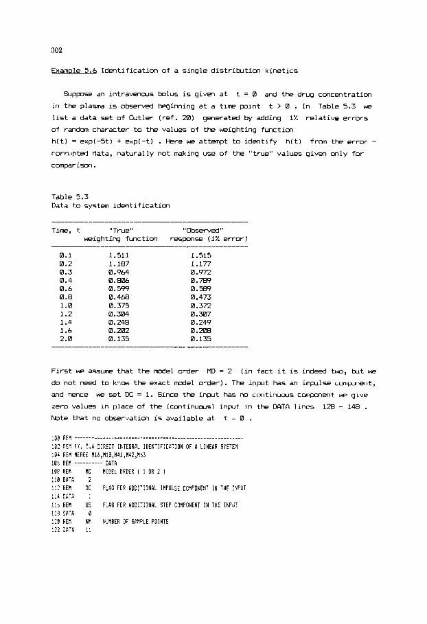
302

Example 5.6 I d e n t i f i c a t i o n of a s i n g l e d i s t r i b u t i o n k i n e t i c s

Suppose an in t r avenous bolus is given a t t = 0 and the drug concentration

i n the plasma is observed beginning a t a time p o i n t t > 0 . In Table 5.3 we

list a d a t a set of Cutler ( r e f . 20) gene ra t ed by adding 1% r e l a t i v e errors

of random c h a r a c t e r to the va lues of the weight ing func t ion

h ( t ) = exp( -5 t ) + e x p ( - t ) . Here we a t t empt to i d e n t i f y h ( t ) from the error -

cor rup ted d a t a , n a t u r a l l y n o t making u s e of t h e " t rue" v a l u e s g iven o n l y f o r

comparison.

Table 5.3 Data t o system i d e n t i f i c a t i o n

T i m e , t "True" "Observed 'I

weighting func t ion response (1% error)

0.1 0.2 0.3 0.4 0.6 0.8 1.0 1.2 1.4 1.6 2.0

1.511 1.187 0.964 0.806 0.599 0.468 0.375 0.304 0.248 O . m 0.135

1.515 1.177 0.972 0.789 0.589 0.473 0.372 0.307 0.249 0 . m 0.135

F i r s t we assume that the model o r d e r MD = 2 ( i n f a c t i t is indeed two, bu t we

do n o t need to know the exact model o r d e r ) . The i n p u t has an impulse component,

and hence we set M3 = 1. S i n c e the i n p u t has no c m t i n u a t s cmponen t we g i v e

z e r o v a l u e s i n p l a c e of the (con t inuous ) i n p l t i n t h e DATA l i n e s 128 - 148 . Note t h a t no obse rva t ion is a v a i l a b l e a t t = 0 .

i;Eg ........................................................... :a? F E 8 EX. 5 .6 DIRECT IKTEClHfiL 1DENTIF:CfiTION OF fi LINEAR SYSTEM ia4 REti RERGE H l b 1 l r l 8 , \ 4 1 , \ 4 2 , \ b 3 :Ci, 4Etl ---------- DATA 10B RE\ ND HODEL SRDES ( 1 OR 2 ) : ID DATfi i :I: RE\ DC FLAG FOR RDDIT!ONfiL INPULSE COMPONENT I N THE INPUT i 3 DATA ! : l b RE! US FLAG FOR ADCITIONRL S T E P COHPCNENT IN THE I N F J '

1 2 F;E1 KI I NURBEF; OF SPKFLE P O I N T S !I! D f i i A 11

113 i a i f i B

303

The first part of the program output c m frun the module M42 of

rmltivariable linear regression. The parameters P(1), P ( 2 ) , P(3) and P(4)

correspond to al, aZr bl and +, respectively, and have no physical meaning.

The weighting function obtained from the estimates is printed as an analytical

expression and its values are also listed.

HULTI'!BRIABLE LINEQR FiEGF'E5510N llETHOD fiF LEOST SQUIRES

305

EIGENVALUE XI 1 1 X ( 2 I XI 3 1 XI 4 I

0.363llEt01 8.520 B.498 -.461 -.518 8.3378BEt00 -.039 8.512 0.814 -.271 0.51837E-BI -.756 R.545 -.352 B.BBB 0.4121BE-B4 8 .395 0.438 0.012 8.887

.---------------------------

WEIGHT Y COHP

0.lB000Et01 0.15150EtR1 0.1flB80Et01 0.11841EtBl 0.1BBBBEt01 0.95536EtBB B.IBBBBEtB1 0.7924BEtBB B.lB000EtBI 0.60182Et88 0.1B000EtBl 0.4bBlbEt0B 8.1BB1BEtBl 8.37347EtB0 1.1B000E+BI 8.38483EtEE B.1000BEt01 B.24917EtBB

0.100B0Et01 0.13745EtB0 B.IUBEBEtB! 8.20467Et08

.__________-_---- RESIDUAL

-.28293E-84 -. 714'27E-02 B. 16641E-Bl -. 34147E-82 -, 12819E-01 8.48361E-82 -.14727E-E? B, 21738E-82 -.19461E-03 B.33343E-82 -. 24493E-82 _________-__----

SUM OF SQUARES ...................... 5.513071E-84 DE6REES OF FREEDOfl .................. 7 STANDARD ERROR ...................... 8.874578E-03 DURBIN-WATSON D-STATISTICS .......... 2.762654 CRITICAL T-VALUE AT 95 1: CDNF. LEVEL 2.37

...................................................................... PRRANETER ESTIHATE ST,ERROR LOWER BOUND UPPER BOUND

P i 1 1 8.59287Et81 0.28378Et08 0.52481Et01 0.65932EtBl P( 2 1 0.47682Et01 0.35937Et80 0.39165Et01 0.56199Et01 P( 5 1 B.15150Et01 0.81448E-02 fl.14957EtUI 8.15343Et01 P( 4 I 0.49347Et01 8.34565EtilE 0.41155E+Bi 0.57539EtBl

CORRELATION MATRIX OF PARAMETERS

MODEL ORDER: '2

IJEIGHTING FUNCTION:

h(t) = Aterp(alfattitBtexp(betattl A = .9578139 R = 1.0591??

a l f a =-.9614869 beta =-4.959159

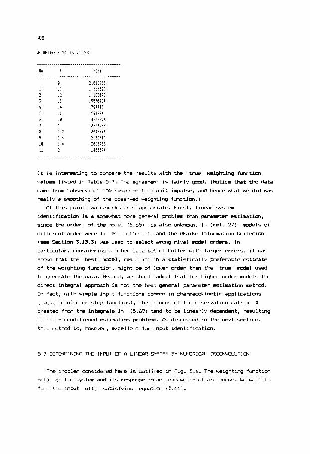
306

I t i s interesting t o canpare the resul ts wi th the "true" weighting func t im

values l i s ted i n Table 5.3. The agreement is f a i r l y gmd. (Notice that the data

came from "observing" the response t o a u n i t impulse, and hence what we d id was

rea l ly a smoothing of the observed weighting function.)

A t t h i s p i n t two remarks are appropriate. F i r s t , l inear system

ident i f icat ion i s a Mmewhat m r e general problem than parameter estimation,

since the order of the model (5.65) i s dl50 unknom. In ( re f . 27) models o f

d i f ferent order were f i t t e d to the data and the Plkaike Information Cr i ter ion

(see Section 3.10.3) was used to select among r i v a l model orders. I n

particular, considering another data set of Cutler wi th larger errors, i t was

shown that the "best" model, resul t ing i n a s t a t i s t i c a l l y preferable estimate

of the weighting function, might be of lower order than the "true" model used

to generate the data. Second, we shwld admit that for higher order models the

direct integral approach i s not the best general parameter estimation method.

In fact, with simple input functions c ~ m m ~ i n pharmacokinetic appl icat ims

(e.g., impulse or step function), the colunns of the observation matrix X

created from the integrals i n (5.69) tend t o be l inear ly dependent, resul t ing

i n ill - conditioned estimation problwm. Fk discussed i n the next section,

t h i s method i s , hOwever, excellent for input ident i f icat ion.

5.7 DETERMINING TK INPUT CF A L INW SYSTEM BY " E R I C & DECOM/OLUTION

The problem considered here i s cutl ined i n Fig. 5 . 6 . The weighting function

h ( t ) of the system and i t s response to an unknown i n p t are known. We want t o

f ind the input u ( t ) sat isfy ing equation ( 5 . 6 6 ) .

307

Co n c e n t ra t io n in the plasma

Absorption U 1 curve

Fig. 5.6. Determining the input correspmding to a given output

Since the cmvolution integral is symmetrical in u(t) and h(t), this

problem is similar to the one of system identification considered in the

previws section. Nevertheless, it is usually easier to find the weighting

function h(t) since its form is m r e - or - less known (e.g., as a sum of

polyexponentials), and hence parametric methods apply, whereas the input

function u(t) is a priori arbitrary. Therefore, the nm - parametric point - area method is a popular way of performing numerical decmvolutim. It is

really simple: evaluating the integral means hl, h2, ..., hn of the weighting

function over the subinterval [ti-l, ti] we can easily solve the set (6.68)

of linear equations for the values El, is,, ..., 5 , of the stepwise input function. A s emphasised in the previws section, this method is, hOwever, very

sensitive to the errors in the o!Jservations. Althwgh we can overcm this

difficulty by carefully smoothing the data (ref. 221, the result will m c h

depend on the particular method of smoothing.

-

Another non - parametric approach is decmvolutim by discrete Fourier

transformatim with built - in windowing. The samples obtained in pharmacokinetic applications are, b v e r , usually short with n m - equidistant

sample time points. Therefore, a variety of parametric decmvolutim methods

have been proposed (refs. 20, 21, 26, 28). In these methods an input of known

form depending on unknown parameters is assumed, and the model response

predicted by the convolution integral (5.66) is fitted to the data.

308

The deconvolution method we propose here i s also parametric and i s based on

d i rect integral parameter estimation ( re f . 27). We consider a "hypothetical"

l inear system S* with input u* = h , where h i s the known weighting

function of the real system S , and the cutplt of

y* = y , the known response function. Then by

S* i s assumed to be

(5.66) we have

Since y* = y , cmparism of equations (5.66) and (5.71) shavs that the

weighting function h* of S* equals the input function u which i s being

scught. NMnl, h' can be estimated by ident i fy ing the weighting function of a

l inear model of the form (5.65) as described i n the previous section. The

sane program can be used fo r input determination i f the ro le of the variables

i s properly understood.

Example 5.7 Determining the absorption curve fo r a given response function

We continue solving the test example of Cutler ( re f . 20). I n Example 5.6 we

ident i f ied the weighting function of the system. Now we consider the second

half of the data set generated by Cutler and shown i n Table 5.4. The "true"

input u ( t ) = l.Zexp(-Zt) and the "true" weighting function were used by Cutler

to generate the "true" response, then 1% random error was added t o obtain the

"observed" response (i.e., the observed drug concentratim i n the plasma). Our

goal i s t o f i nd the input (i.e., the absorption curve) making use of the

weighting function ident i f ied i n the previous example and the "observed"

response.

Table 5.4 Data t o determine the absorDtion curve

Time, t "True" "True" 'I Observed 'I input response respMse (1% error)

0 0.1 0.2 0.3 0.4 0.6 0.8 1.0 1.2 1.4 1.6 2.0

1.2 0.9825 0.8044 0.6586 0.5392 0.3614 0.2423 0.1624 0.1089 0.0733 0.0489 0.0i-m

0 0.1m 0.293 0.3M 0.394 0.4caCa 0.368 0.327 0.288 0.252 0.211 0.155

0 0.181 0.291 0.361 0.388 0.399 0.372 0.328 0.286 0.249 0.210 0.153

309

W h e n i d e n t i f y i n g t h e hypo the t i ca l s y s t m S* we need u* . The weight ing

func t ion found i n Example 5.6 is s u b s t i t u t e d f o r the i n p t of the hypo the t i ca l

system. Th i s i n p u t does n o t c o n t a i n an impulse or a u n i t s t e p cmponent, and

hence we set M3 = 0 and US = 0 . The response of the hypo the t i ca l sys tem

e q u a l s t h e "Observed" response. The program is the me used i n Example 5.6,

on ly t h a d a t a l i n e s are changed as fo l lows:

T h e assumed model o r d e r is ND = 1 . We list here m l y t h e essential parts of

the rxltput.

_._.....___________---------------------

! E E L OKCER: 1

310

The "weighting function" we fwnd is that of the hypothetical system,

therefore it is the absorption curve we were looking for. It is useful to

compare it with the "true" input given in Table 5.4. In this special case the

input function fwnd and the "true" input are of the same analytical form, so

we can compare the parameters of the two functions, as well. In realistic

applications, however, we are not interested in the "analytical form" of the

inplt function and rather the table of computed values is of primary interest.

The direct integral approach to numerical deconvolution preserves the

symmetry of system identification and input determination, similarly to the

point - area method. By (5.71) the inplt function u = ht is restricted to

the class of weighting functions generated by a single - inpt, single -

outplt, time invariant system (5.65). This class includes plyexponmtials,

polynomials and trigmometric functions, so that the constraint on the form of

the inpt is relatively mild. This constraint may in fact have a physical

meaning in pharmacokinetics. For example, in the problem studied in Example 5.7

the hypotetical system Sx

bioavailability of the drug following an impulse administration via an

extravascular route.

may be a real linear system whose response is the

Exercise

0 Repeat the input identification experiment with the model order MD = 2 . Cwnpare the linear regression residual errors for the two cases. Select the

"best" model order on the basis of the Akaike Information Criterion (5-

Section 3.10.3 and ref. 27) .

311

5.8 WPLICATIaVS W D NRHTER PRoBLOls

5.8.1 Principal comment analysis of kinetic models

The researcher usually looks for a model that not only fits the data well,

but describes the mechanism of action of the chemical or biological process.

Such detailed models are, however, frequently overparameterized with respect tn

the available data, leading to ill-conditioned pi-nblems of parameter

estimation. In Sectim 3.5.2 you have learned that principal component analysis

of the normalized cross-product matrix J T ( p ) W ( p )

detecting ill-conditioned parameter estimation problems. In Section 5.3 w e

introduced the matrix S of normalized sensitivity coefficients. It plays the

same role for dynamical models as J(i0) in algebraic parameter estimation

problems. Therefore, the principal compmmt analysis of STS (or of STWS , if weighting is necessary) offers a convenient twl for extracting information

from sensitivity coefficients, and it reveals whether or not there is any hope

to identify the parameters of the model. Although we need initial parameter

estimates to perform the calculation, such are usually available in the

literature, at least in the form of sane order of magnitude guesses. In this

section we reconsider the sensitivity coefficients obtained in Example 5.3.

is a standard method of

Example 5.8.1 Practical idmtifiability of the parameters of the microbial

gravth process

As sham by Holmberg (ref. 3) the four parameters Vm, K,, Kd and Y are

theoretically identifiable if both the concentration of the microorganism

and that of the substrate

parameters is, hmever, a rmch more difficult issue. In the following four

cases are investigated:

(yl) are observed. Practical idmtifiability of the (yz)

(i) Both concentrations, y1 and yz are observed. The error variance is

small: 2 = 0.01 .

(ii) Both y1 and yz are observed. The error variance is large: 6' = 1 .

(iii) Gnly the substrate, yz is observed. The error variance is c? = 0.01 .

(iv) bly yz is observed. The error variance is 2 = 1 .

To investigate cases (i) and (ii), the S matrix obtained in Example 5.3 is

used directly. Forming STS and applying eigenvalue-eigmvector decomposition

(by the module M18), we obtain the results show, in Table 5.5.

312

Table 5.5 Principal component analysis of the normalized sensitivity matrix; both concentrations observed

Eigenvalue Eigenvector components corresponding to vln KS Kd Y

69429 0.957 -0.134 -0.095 -0.239 12304 0.230 0.020 -0.137 0.963

2.583 0.042 -0.518 0.846 0.121 1.724 0.172 0.845 0 .37 0.013

In case (i) l W a 2 = 1 , and hence the problem is not ill-conditioned, all

the parameters can be identified. Lhfortunately we can hardly hope such a small

error variance in biotechnical applications. In the more realistic case (ii)

l W a 2 = 100 , thus two eigenvalues are below the threshold. As it was discussed

in Section 3.5, the eigenvectors corresponding to the small eigenvalues show

that there is no hope to identify parameters Ks and Kd with reasonable

accuracy.

To investigate cases (iii) and (iv), we include only every second r w of

matrix S obtained in Example 5.3 w h e n forming STS . Plpplying eigenvalue- eigenvector decomposition again, the results shown in Table 5.6 are obtained.

Table 5.6 Principal compcnent analysis of the normalized sensitivity matrix; only substrate y2 is observed

--------________________________________----___------_ Eigenvalue Eigenvector cmponents corresponding to

Vm KS Kd Y

51599 0.912 -0.137 -0.DBl -0.378 19.225 0.334 -0.225 -0.097 0 . W 0.409 0.212 0.964 0 . W 0.162 0 . m 7 0.10-5 -0.041 0.991 0.057

As seen from the table, in case (iii) we can identify V, and Y , but neither K, nor Kd can be estimated. In the (unfortunately) more realistic

case (iv) one can hope a reasonable parameter estimate only for V,. It is

advantageous to fix all the other parameters at s m e nominal value, so avoiding

the inherent difficulties of the parameter estimation process.

Practical identifiability is not the only problem that can be adressed by

principal compcnent analysis of the sensitivity matrix. In (refs. 29-30)

several examples of model reduction based on this technique are discussed.

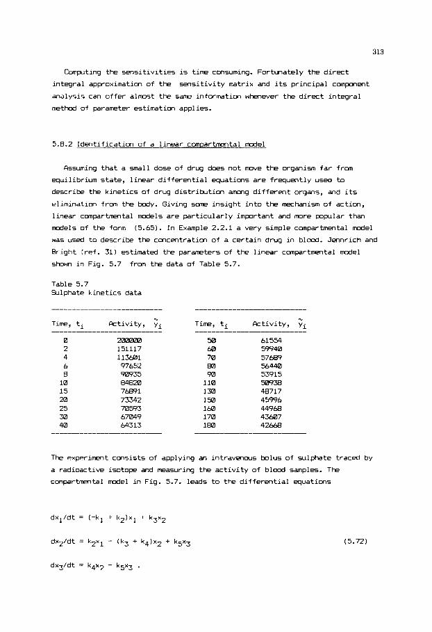
313

Computing the sensitivities is time consuming. Fortunately the direct

integral approximation of the sensitivity matrix and its principal compment

analysis can offer almost the same information whmever the direct integral

method of parameter estimation applies.

5.8.2 Identification of a linear compartmental model

Assuming that a small dose of drug does not m v e the organism far from

equilibrium state, linear differential equations are frequently used to

describe the kinetics of drug distribution a m g different organs, and its

elimination from the body. Giving some insight into the mechanism of action,

linear compartmental models are particularly important and m r e popular than

models of the form (5.65). In Example 2.2.1 a very simple cmpartmmtal model

was used to describe the concentration of a certain drug in blwd. Jennrich and

Bright (ref. 31) estimated the parameters of the linear campartmental model

shown in Fig. 5.7 from the data of Table 5.7.

Table 5.7 Sulphate kinetics data

Time, -_____ 0 2 4 6 8 10 15 20 25 30 40

.”

ti Activity, yi

2m0m 151117 113601 97652 90935 84820 74991 73342 70593 67049 64313

.”

Time, ti Fktivity, yi

50 60 70 60 90 110 132 150 160 170 160

61554 59940 57689 564m 53915 5093 40717 45996 44968 43607 42668

The experiment consists of applying an intravenous bolus of sulphate traced by

a radioactive isotope and measuring the activity of blwd samples. The

compartmental &el in Fig. 5.7. leads to the differential equations

(5.72)

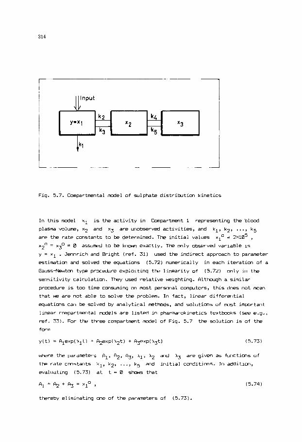
314

Fig. 5.7. Canpartmental model of sulphate distribution kinetics

In this model x1 is the activity in Cmpartment 1 representing the blood

plasm volume, x2 and x3 are unobserved activities, and kl, k2, ..., k5 are the rate constants to be determined. The initial values

x20 = xJO = 0

y = x1 . Jennrich and Bright (ref. 31) used the indirect approach to parameter estimation and solved the equations (5.721 numerically in each iteration of a

Gauss-Newton type procedure exploiting the linearity of (5.72) only in the

sensitivity calculation. They used relative weighting. Altbgh a similar

procedure is too time consuming on most personal complters, this does not mean

that w e are not able to solve the problem. In fact, linear differential

equations can be solved by analytical methods, and solutions of most important

linear compartmental models are listed in pharmacokinetics textbooks ( s e e e . g . ,

ref. 33). For the three compartment model of Fig. 5.7 the solution is of the

f orm

xIo = ZXlD5 , assumed to be known exactly. The only observed variable is

where the parameters Al, A2, A3, XI, X2 and X3 are given as functions of

the rate constants kl, k2, ..., k5 and initial conditions. In addition,

evaluating (5.73) at t = 0 shcws that

A1 + + + % = x10 , (5.74)

thereby eliminating one of the parameters of (5.73).

315

Now we can proceed i n two d i f f e r e n t ways, either by e s t ima t ing the

parameters k l , k2, ..., k5 d i r e c t l y , u s ing the a n a l y t i c a l s n l u t i o n and the

module M45, or e s t ima t ing f i r s t the parameters i n (5.73). In t h i s latter

case we can use the very s imple peel ing method, also known a5 the method of

r e s i d u a l s . A l thwgh the pee l ing procedure is of approximate character and does

n o t t a k e i n t o account t h e a v a i l a b l e c o n s t r a i n t s such a5 (5.741, it s t i l l g i v e s

use fu l i n i t i a l estimates f o r the least s q u a r e s method.

T h e peel ing method is based on the obse rva t ion that f o r compartmental models

Xi < 0

n o t close to each other, s i n c e otherwise we are unab le to s e p a r a t e the terms of

(5.73) and m u s t lump s e v e r a l compartments. A s s u m e that the i n e q u a l i t i e s

X1 < h2 < X3 < 0

i n the s o l u t i o n s of t h e form (5.73). In a d d i t i o n , the exponents are

hold, t h m the peel ing c o n s i s t s of the fol lowing steps:

( i ) Divide the time i n t e r v a l i n t o 3 s u b i n t e r v a l s , con ta in ing nl, n2 and

n3 sample p i n t s .

p o i n t s , r e s p e c t i v e l y , w h e r e n1 + n2 + n3 = n , the total number of

(ii) S ince X1 and X2 are sma l l e r than X3, w e may assume t h a t i n the last

s u b i n t e r v a l the c o n t r i b u t i o n from the f i r s t two exponents is small.

Therefore ,

* log yi z log + hJ t i , i = n1 + n2 + 1, ..., n , (5.75)

and % and X3 can be found by f i t t i n g a s t r a i g h t l i n e to the last

n3 p o i n t of the da ta .

(iii) In the second s u b i n t e r v a l on ly the f i r s t term of (5.73) is assumed to

be small, but +xp(A3ti) is a l r e a d y k n m from (ii). Thus aga in

a s t r a i g h t l i n e is f i t t e d to the d a t a

log[;. - A exp(X t 11 z log A + X 2 t i , i = n + 1, ..., n + n 1 3 3 i 2 1 1 2 ’

(5.76)

thereby e s t ima t ing % and X2.

( i v ) F i n a l l y , a s t r a i g h t l i n e is f i t t e d to the d a t a

i n o r d e r to e s t i m a t e A1 and X1.

T h e c r i t i ca l p o i n t i n the peel ing technique is the r i g h t choice o f

n2 . By (5.75)

n3 and

the logar i th ized obse rva t ions are close to a s t r a i g h t l i n e i n

316

the last subinterval, and hence a semi - lcqarithic plot of the data helps to

find the value of

values log[yi - A3exp(h3ti)l may help to choose n2 . For the data of Table 5.7 we select n1 = 6, n2 = 8 and n3 = 8 . Since relative error i5 assumed in the original data, unit weights are used when fitting the logarithic data

(see Section 3.4), and hence the modul M40 applies. The resulting estimates

are

n3 . A similar plot of the corrected and logarithized

*

A1 = l.WXlD5 , + = 2.19~10~ , A3 = 6.93~10~ , X i = -.313 , h2 = 43.0562 'A3 = -0.0027 .

These values are further refined by the module M45 applying relative

'c

weighting wi = l /yi2 and eliminating A-J by (5.74). The following estimates

and standard errors are obtained

The weighted residual sum of squares is Q = 0.00284 , close to the value Q = 0 . m 7 of Jennrich and Bright. Thus the fit is satisfying and the

peeling method is 5- to give surprisingly good initial estimates. The only

remaining problem is to find the values of the original parameters

kl, k2, ..., k5. This can be done via the formulas listed in (ref. 32)

where

The final estimates

317

kl = 0.0754 , k 2 = 0.1754 , k3 = 0.1351 , k4 = 0.0156 and kg = 0.04m

agree well with the ones of Jmnrich and Bright (ref. 31).

Exercises

0 Carry w t numerical experiments with other choices of n1 , n2 and n3 in

the peeling method. Try to construct a heuristic rule for subinterval

selection which can be used in a computer without hwnan interaction.

Compute approximate standard errors of the parameters kl, k2, ..., k5 , using the error propagation law

2

REFERu\K3ES

1 P. Henrici, Discrete Variable Methods in Ordinary Differential Equations,

2 R.L. Joinston, hmerical Methods, A Software Approach, John Wiley,

3 A. Holmberg, the practical identifiability of microbial growth models

John Wiley, New York, 1962.

New York, 1982.

incorporating Michaelis-Menten type Nonlinearities, Mathematical Bioscimces, 62 (1982) 23-43.

4 B. Carnahan and J.O. Wilkes, Digital Cmputing and r\lunerical Methods, Join Wiley, New York, 1973.

5 E. Fehlberg, Klassi~he Runge-Kutta-Forrrula fiinfter und siebenter Ordung mit Schrittweitm-Kontrolle, Computing, 4 (1969) 93-1m6.

6 C.W. Gear, The automatic integration o f ordinary differential equations. Communications of the AavI, 14 (1971) 176-180.

7 P. Seifert, Compltational experiments with algorithns for stiff ODES, hputing, 38 (1987) 163-176.

E B.A. Gottwald and G. Wanner, A reliable Rosenbrock-integrator for stiff differential equations, Computing, 26 (1981) 335-357.

9 R.J. Field and R.M. Noyes, Oscillations in chemical systems. J. Chemical Physics, 60 (1974) 1877-1884.

10 H. Rabitz, Sensitivity analysis: Thwry with applications to molecular dynamics and kinetics. Computers and Chemistry, 5 (1960) 167-180.

11 R.P. Dickinson and R.J. Gelinas, Sensitivity analysis of ordinary differential equation, J. Comp. Physics, 21 (1978) 123-143.

12 A.M Dunker, The decoupled direct method for calculating sensitivity coefficients in chemical kinetics, J. Chem. Phys. 81 (1984) 2385-2393.

13 P. Valkb and S. Vajda, Pn extended ODE solver for sensitivity calculations, Computers and Chemistry, 8 (1984) 255-271.

318

14 R.A. Alberty and F. Daniels, Physical Chmistry 5th ed. John Wiley,

15 Y. Bard, Nonlinear Parameter Estimatim. Academic Press, NEW York, 1974. 16 D.M. Himlblau, C.R: Jones and K.B. Bixhoff, Determination of rate

NEW York, 1980.

constants for complex kinetic dels, Ind. Eng. Chm. Fundamentals, 6 (1967) 539-546.

17 A. Yermakova, S. Vajda and P. Valkb, Direct integral method via spline approximation for estimating rate constants. Applied Catalysis, 2 (1982) 139-1E0.

18 S. Vajda, P. Valkb and K.R. Godfrey, Direct and indirect least squares methods in continuous-time parameter estimation, k t m t i c a , 23 (1987) 707-718.

19 F.K. Uno, H.L. Ralston, R.I. Jennrich and P.F. Sampsm, Test problw from the pharmacokinetic literature requiring fitting models defined by differential equations, Technical Report No. 61. WlW Statistical Software, Los Fhgeles, 1979.

20 D.J. Cutler, b r i c a l decmvolutim by least squares: Use of prescribed input functions, J. Pharmacokinetics and Biopharm., 6 (19781 227-242.

21 D.J. Cutler, Mmerical decmvolution by least squares: Use of polynomials to represent input function. J. Pharmacokinetics and Biopharm., 6 (1978) 243-263.

22 F. Langenbucher, Numerical convolutim/decmvolution as a tool for correlating in vitro with in vivo drug availability, Pharm. Ind., 44 (1962) 1166-1172.

23 C.T. Chen, Introduction to Linear System Theory, Holt, Rinehart and Winston, NEW York, 1970.

24 D.P. Vaughan and M. Dennis, Mathematical basis for the point-are dKCnvOlUtiM method for determining in vivo input functions. J. Phar. Sci., Part I, 69 (1960) 298-305, Part 11, 69 (1960) 663-665

systwm, Math. Bioscimces, 10 (1971) 215-237.

systems with plyexponential impulse response, J. Pharm. Sci., 69 (1980) 312-318.

identification methods, J. Pharmacokinetics and Biopharm., 16 (1988) 85-107.

linear pharmacokinetics. J. Phar. Biopharm, 8 (19EQl) 463-481.

models, Int. J. Chem. Kinet. 17 (1985) 55-81.

Edelsm-Field-Noyes mcdel of Belousov-Zhabotinsky reactim, J. Phys. C h m . 90 (1986) 1664.

31 R.I. Jennrich and P.B. Right, Fitting s y s t w of linear differential equations using computer generated exact derivatives, Technomtrics, 18 (1976) 385-399.

25 B.R. hnt, Biased estimation for nmparametric identification of linear

26 P. Veng-Pdersen, Novel deconvolutim method for linear pharmacokinetic

27 S. Vajda, K.R. Gcdfrey and P. Valkb, kmerical decmvolution using system

28 P. Veng-Pedersm, I% algorithm and computer program for deconvolutim in

29 S.Vajda, P. Valk6 and T. Turdnyi, Principal component analysis of kinetic

Je, S. Vajda and T. Turdnyi, Principal component analysis for reducing the

32 M.S. Gibaldi and D.Perrier, Pharmacokinetics, Marcel Dekker, N e w York, 1975.

319

SUBJECT I N D E X

absorption curve 306 abstract factors 65 accelerating factor 99 acid-catalysed reaction 158, 179 activity coefficient 127 addition of zeros 253 affine linear relationship 62, 186 Aitken form 227 Akaike's Information Criterion

Akima method 257 aliasing of the spectrum 250 Almdsy indicator 189, 192 Pntoine equation 214 Arrhmius dependence 173, 182 artificial variables 20 atom matrix 48, 131 -, virtual 48, 133

213, 306

background absorption 56 backsubstitution 28, 32 balance equation, linear 188

base line correction 253 basis 4

Belousov-Zhabotinsky reaction 277 bisecticn method 74 blending problem 13, 24 Box - Draper method 184 boxcar function 246 bracketing interval 74 Brent method 96 broadening of the spectrum 254) Broyden method 107, 119, 128

canonical basis 5, 7, 16 canonical form 59 Cardano method 71 charge balance equation 125 Ckbysev approximation 54 chemical reaction 47, 102 chi square distribution 154, 189 Cholevsky method 35, 197 compartmental model 91, 313 condition number 4.5, 60 confidence interval 147 confidence r q i m 144, 154, 178 convergence, motonic 86

conversion 59 convolution 247, 253, 298 coordinate transformation 6 correlation coefficients 1.53 covariance matrix 63, 153, 163 cross product matrix, normalized

-, nonlinear 193

- variable 11

-, oscillating 86

164, 182, 311

curtosis 210 cut-off method 88 cycling 19

damped iteration 99 Davidon-Fletcher-Powell method 119 deconvolution 298, 307 determinant 29, 31 - criterion 184 diagonal dominance 39 diagonal matrix 42 dimension 4 Dirac impulse 248, 300 direct integral method 284, 3aM direct search method 112 discriminant 71 dissociation reaction 125 distribution kinetics 302 divergence, motonic 86

divided difference 225 drug dosing 91 Durbin - Wattson D-statistics 152

eigenanalysis 41 electronic absorption spectrum 258 enthalpy 226, 239 enzyme reaction 123, 177, 283 equilibrium condition 128 equilibrium relations 102, 125 equivalence point, detection of 231 error measure 189 error propagation 317 estimation criterion 140 Euler method, explicit 263

experiment design, A - optimal 211

-, oscillating 86

-, implicit 265 -, D - optimal 211, 212 -, E - optimal 211 extent of reaction 48 extract 127 extrapolation 228

F-test 146, 152 false position method 77 Fast Fourier Transformation 2321 feasible solution 15 Fibonacci search 96 FLEPaVlIN program 119 Forsythe polynomials 205 Fourier transformation 24.5 -, cmtinuous 247 -, discrete 249, 298, 3BB free variable 11 frequmcy d m i n 240 full pivoting 13

320

Gauss-Newton-Marquardt method

Gaussian elimination 27, 36, 39 Gaussian function 223, 254, 258 Gear program 273 Gibbs free energy 127, 131 golden section 68, 98 gradient method 112

Hausholder formula 108, 111 Hessian matrix 112, 173 Hilbert matrix 37, 61

195, 164

ill-conditioned problem

indicator variable 16 inverse matrix 12 inverse transform 247, 249 iterative improvement 46 iterative reweighting 196 isomerization of alpha-pinene

45, 178, 282, 3e)6

61, 185

Jacobi method 42 Jacobian matrix 105, 162, 274, 288

Lagrange formula 224 Lagranqe multiplier 132, 188, 241 least absolute deviations 51 least squares 58, 140, 258, 289 Levenberg-Marquardt modification 163 linear combination 3 linear dependence 61 linear interpolation 210 linear system 297 linearization, Eadie-Hofstee 176 -, Hanes 176 -, Lineweaver--Wlrk 176 -, Scatchard 176 linearly dependent vectors 4 linearly independent vectors 4 lower triangular matrix 27 LU decomposition 28, 131

Margules equation 127, 164 Marquardt parameter 163, 179 mass balance equation 125 material balance 128 matrix inverse 2, 12, 34 maximum likelihood principle

method of residuals 315 Michaelis - Mmten equation

Milne method 270 minimax criterion 54, 210 multiresmse estimatim 61

141, 194

123, 176, 268, 294

Newton formula 2251 Newton method 112, 241

Newton-Raphson method 82, 104, 130 normal distribution 144, 210 normal form 15 normalized eigenvectors 41 Nyquist critical frequency 2%

odd multiplicity 75 ordinary differential equation 261

Oregmator model 277 orthogonal polynomials 225, 228 orthonormal eigenvectors 41 outlier 55, 210 overrelaxation 99

Oregonator model 277 orthogonal polynomials 205, 228 orthonormal eigenvectors 41 outlier 55, 210 overrelaxation 99

partial pivoting 13 peeling method 315 Peng-Robinson equation of state 72 permutation matrix 27, 29 phax equilibrium 129 pivot element 6, 9, 343 point-area method 299, 307 polynomial equation 126 positive definite matrix 35, 119 potenticmetric titration 232, 254 practical identifiability 311 predictor-corrector method 269 principal component analysis

65, 183, 282, 311

quadratic form 35, 188 quasi Newton method 107 quasi steady state approximation

124, 283

radiographic investigation 2(2w

raffinate 127 RAM) algorithm 133 random number 144 reaction invariants 51, 133 reaction matrix 47 -, virtual 48 regression line 145 residual 45, 143 response function 59, 139 -, virtual 197 restricted equilibrium 133 ridge parameter 155, 179 ridge regression 179 Rosmbrock function 117, 121 Rosenbrock method 273 m 4 A 273 Runge-Kutta method 265 -, m i implicit 273

321

saddle point 59 Savitzky - Golay

scalar product 1

Weigstein method 99

weighting function 298, 339 weighting matrix 187 weighting, Poisson 161

window function 258

f ormu 1 a weighting coefficients 145, 174 229, 231, 253

scaling of the parameters 155 secant method m sensitivity coefficient 278 -, semi-logarithmic 281 sensitivity equation 279 sensitivity matrix 281 stladow price 24, 137 signal-to-noise ratio 221 similarity transformation 41 simplex 113 simplex method of Nelder and Mead

simplex tableau 19 Simpson rule 234 singular value 61 singularity 37 slack variables 15, i0 solving a matrix equation J3 spectroscopy 56 spectrum, amplitude 248

-, relative 148, 155, 169

113, 187

-, phase 248 -, power 248 -, interpolating 235, S02 -, natural 236, 241, 287 -, smothing 240 stability 265 standard error 146 steepest descent method 112 step size 272 stiff differential equation 273 stoichimtric coefficient 47 rjtoichiwnetric number of freedom 48 stoichimtric subspace 47 stoichimtry 47 Student's t distributim 57, 147

spline, cubic 236, 287

, subspace 3 1 successive approximation 85, 99

symmetric matrix 35, 41

Taylor series 265 Thomas algorith 39 trapezium rule 234, 249 tridiagmal matrix equation 39

unimdal function 87 unit vector 4 updating formla lB8, 119 upper triangular matrix 27 user supplied subrwtine 76

van Laar parameters 215 vapor pressure 73, 207, 214 vapor-liquid equilibrium 214 vector coordinates 2

This Page Intentionally Left Blank