Data-driven performance analyses of wastewater treatment ...

lable at ScienceDirect

Water Research 157 (2019) 498e513

Contents lists avai

Water Research

journal homepage: www.elsevier .com/locate/watres

Review

Data-driven performance analyses of wastewater treatment plants: Areview

Kathryn B. Newhart a, Ryan W. Holloway b, Amanda S. Hering c, *, Tzahi Y. Cath a, **

a Department of Civil and Environmental Engineering, Colorado School of Mines, Golden, CO, 80401, USAb Kennedy/Jenks Consultants, Rancho Cordova, CA, 95670, USAc Department of Statistical Science, Baylor University, Waco, TX, 76798, USA

a r t i c l e i n f o

Article history:Received 9 September 2018Received in revised form12 March 2019Accepted 16 March 2019Available online 21 March 2019

Keywords:Wastewater treatmentBig dataStatistical process controlProcess optimizationMonitoring

* Corresponding author.** Corresponding author.

E-mail addresses: [email protected] (A.S.

https://doi.org/10.1016/j.watres.2019.03.0300043-1354/© 2019 Elsevier Ltd. All rights reserved.

a b s t r a c t

Recent advancements in data-driven process control and performance analysis could provide thewastewater treatment industry with an opportunity to reduce costs and improve operations. However, bigdata inwastewater treatment plants (WWTP) is widely underutilized, due in part to a workforce that lacksbackground knowledge of data science required to fully analyze the unique characteristics of WWTP.Wastewater treatment processes exhibit nonlinear, nonstationary, autocorrelated, and co-correlatedbehavior that (i) is very difficult to model using first principals and (ii) must be considered whenimplementing data-driven methods. This review provides an overview of data-driven methods ofachieving fault detection, variable prediction, and advanced control of WWTP. We present how big datahas been used in the context of WWTP, and much of the discussion can also be applied to water treatment.Due to the assumptions inherent in different data-driven modeling approaches (e.g., control charts, sta-tistical process control, model predictive control, neural networks, transfer functions, fuzzy logic), not allmethods are appropriate for every goal or every dataset. Practical guidance is given for matching a desiredgoal with a particular methodology along with considerations regarding the assumed data structure.References for further reading are provided, and an overall analysis framework is presented.

© 2019 Elsevier Ltd. All rights reserved.

Contents

1. Introduction . . . . . . . . . . . . . . . . . . . . . . . . . . . . . . . . . . . . . . . . . . . . . . . . . . . . . . . . . . . . . . . . . . . . . . . . . . . . . . . . . . . . . . . . . . . . . . . . . . . . . . . . . . . . . . . . . . . . . . 4992. Background . . . . . . . . . . . . . . . . . . . . . . . . . . . . . . . . . . . . . . . . . . . . . . . . . . . . . . . . . . . . . . . . . . . . . . . . . . . . . . . . . . . . . . . . . . . . . . . . . . . . . . . . . . . . . . . . . . . . . . 499

2.1. Big data . . . . . . . . . . . . . . . . . . . . . . . . . . . . . . . . . . . . . . . . . . . . . . . . . . . . . . . . . . . . . . . . . . . . . . . . . . . . . . . . . . . . . . . . . . . . . . . . . . . . . . . . . . . . . . . . . . . . . 4992.2. Water & wastewater treatment . . . . . . . . . . . . . . . . . . . . . . . . . . . . . . . . . . . . . . . . . . . . . . . . . . . . . . . . . . . . . . . . . . . . . . . . . . . . . . . . . . . . . . . . . . . . . . . 5002.3. Data considerations . . . . . . . . . . . . . . . . . . . . . . . . . . . . . . . . . . . . . . . . . . . . . . . . . . . . . . . . . . . . . . . . . . . . . . . . . . . . . . . . . . . . . . . . . . . . . . . . . . . . . . . . . . 500

2.3.1. Structure . . . . . . . . . . . . . . . . . . . . . . . . . . . . . . . . . . . . . . . . . . . . . . . . . . . . . . . . . . . . . . . . . . . . . . . . . . . . . . . . . . . . . . . . . . . . . . . . . . . . . . . . . . . . 5002.3.2. Frequency and temporal variability . . . . . . . . . . . . . . . . . . . . . . . . . . . . . . . . . . . . . . . . . . . . . . . . . . . . . . . . . . . . . . . . . . . . . . . . . . . . . . . . . . . . . 5012.3.3. Variable characteristics . . . . . . . . . . . . . . . . . . . . . . . . . . . . . . . . . . . . . . . . . . . . . . . . . . . . . . . . . . . . . . . . . . . . . . . . . . . . . . . . . . . . . . . . . . . . . . . 501

2.4. Exploratory data analysis . . . . . . . . . . . . . . . . . . . . . . . . . . . . . . . . . . . . . . . . . . . . . . . . . . . . . . . . . . . . . . . . . . . . . . . . . . . . . . . . . . . . . . . . . . . . . . . . . . . . . 5023. Methods & examples . . . . . . . . . . . . . . . . . . . . . . . . . . . . . . . . . . . . . . . . . . . . . . . . . . . . . . . . . . . . . . . . . . . . . . . . . . . . . . . . . . . . . . . . . . . . . . . . . . . . . . . . . . . . . . 503

3.1. Historical process control . . . . . . . . . . . . . . . . . . . . . . . . . . . . . . . . . . . . . . . . . . . . . . . . . . . . . . . . . . . . . . . . . . . . . . . . . . . . . . . . . . . . . . . . . . . . . . . . . . . . . 5033.2. Fault detection . . . . . . . . . . . . . . . . . . . . . . . . . . . . . . . . . . . . . . . . . . . . . . . . . . . . . . . . . . . . . . . . . . . . . . . . . . . . . . . . . . . . . . . . . . . . . . . . . . . . . . . . . . . . . . 503

3.2.1. Control charts . . . . . . . . . . . . . . . . . . . . . . . . . . . . . . . . . . . . . . . . . . . . . . . . . . . . . . . . . . . . . . . . . . . . . . . . . . . . . . . . . . . . . . . . . . . . . . . . . . . . . . . . 5033.2.2. Principal component analysis . . . . . . . . . . . . . . . . . . . . . . . . . . . . . . . . . . . . . . . . . . . . . . . . . . . . . . . . . . . . . . . . . . . . . . . . . . . . . . . . . . . . . . . . . . 5043.2.3. Partial least squares . . . . . . . . . . . . . . . . . . . . . . . . . . . . . . . . . . . . . . . . . . . . . . . . . . . . . . . . . . . . . . . . . . . . . . . . . . . . . . . . . . . . . . . . . . . . . . . . . . 5053.2.4. Neural networks . . . . . . . . . . . . . . . . . . . . . . . . . . . . . . . . . . . . . . . . . . . . . . . . . . . . . . . . . . . . . . . . . . . . . . . . . . . . . . . . . . . . . . . . . . . . . . . . . . . . . 506

3.3. Variable prediction . . . . . . . . . . . . . . . . . . . . . . . . . . . . . . . . . . . . . . . . . . . . . . . . . . . . . . . . . . . . . . . . . . . . . . . . . . . . . . . . . . . . . . . . . . . . . . . . . . . . . . . . . . 506

Hering), [email protected] (T.Y. Cath).

mailto:[email protected]

mailto:[email protected]

http://crossmark.crossref.org/dialog/?doi=10.1016/j.watres.2019.03.030&domain=pdf

www.sciencedirect.com/science/journal/00431354

www.elsevier.com/locate/watres

https://doi.org/10.1016/j.watres.2019.03.030



K.B. Newhart et al. / Water Research 157 (2019) 498e513 499

3.3.1. Activated sludge models . . . . . . . . . . . . . . . . . . . . . . . . . . . . . . . . . . . . . . . . . . . . . . . . . . . . . . . . . . . . . . . . . . . . . . . . . . . . . . . . . . . . . . . . . . . . . . 5073.3.2. Transfer function models . . . . . . . . . . . . . . . . . . . . . . . . . . . . . . . . . . . . . . . . . . . . . . . . . . . . . . . . . . . . . . . . . . . . . . . . . . . . . . . . . . . . . . . . . . . . . 5073.3.3. Multiple regression . . . . . . . . . . . . . . . . . . . . . . . . . . . . . . . . . . . . . . . . . . . . . . . . . . . . . . . . . . . . . . . . . . . . . . . . . . . . . . . . . . . . . . . . . . . . . . . . . . . 5073.3.4. Neural networks . . . . . . . . . . . . . . . . . . . . . . . . . . . . . . . . . . . . . . . . . . . . . . . . . . . . . . . . . . . . . . . . . . . . . . . . . . . . . . . . . . . . . . . . . . . . . . . . . . . . . 508

3.4. Advanced control . . . . . . . . . . . . . . . . . . . . . . . . . . . . . . . . . . . . . . . . . . . . . . . . . . . . . . . . . . . . . . . . . . . . . . . . . . . . . . . . . . . . . . . . . . . . . . . . . . . . . . . . . . . . 5083.4.1. Model predictive control . . . . . . . . . . . . . . . . . . . . . . . . . . . . . . . . . . . . . . . . . . . . . . . . . . . . . . . . . . . . . . . . . . . . . . . . . . . . . . . . . . . . . . . . . . . . . . . 5083.4.2. Neural networks . . . . . . . . . . . . . . . . . . . . . . . . . . . . . . . . . . . . . . . . . . . . . . . . . . . . . . . . . . . . . . . . . . . . . . . . . . . . . . . . . . . . . . . . . . . . . . . . . . . . . 5093.4.3. Transfer function models . . . . . . . . . . . . . . . . . . . . . . . . . . . . . . . . . . . . . . . . . . . . . . . . . . . . . . . . . . . . . . . . . . . . . . . . . . . . . . . . . . . . . . . . . . . . . 5093.4.4. Fuzzy logic . . . . . . . . . . . . . . . . . . . . . . . . . . . . . . . . . . . . . . . . . . . . . . . . . . . . . . . . . . . . . . . . . . . . . . . . . . . . . . . . . . . . . . . . . . . . . . . . . . . . . . . . . . 510

4. Conclusions and recommendations . . . . . . . . . . . . . . . . . . . . . . . . . . . . . . . . . . . . . . . . . . . . . . . . . . . . . . . . . . . . . . . . . . . . . . . . . . . . . . . . . . . . . . . . . . . . . . . . . . 510Acknowledgments . . . . . . . . . . . . . . . . . . . . . . . . . . . . . . . . . . . . . . . . . . . . . . . . . . . . . . . . . . . . . . . . . . . . . . . . . . . . . . . . . . . . . . . . . . . . . . . . . . . . . . . . . . . . . . . . 510Acronyms . . . . . . . . . . . . . . . . . . . . . . . . . . . . . . . . . . . . . . . . . . . . . . . . . . . . . . . . . . . . . . . . . . . . . . . . . . . . . . . . . . . . . . . . . . . . . . . . . . . . . . . . . . . . . . . . . . . . . . . . . 511References . . . . . . . . . . . . . . . . . . . . . . . . . . . . . . . . . . . . . . . . . . . . . . . . . . . . . . . . . . . . . . . . . . . . . . . . . . . . . . . . . . . . . . . . . . . . . . . . . . . . . . . . . . . . . . . . . . . . . . . . 511

1. Introduction

Municipal wastewater treatment plants (WWTP) continuouslymonitor and collect data from unit processes, but the data are oftenunderutilized. Due to the size and complexity of datasets currentlygenerated by WWTP and the lack of data science background forWWTP professionals, it can be challenging to efficiently collect,manage, and analyze the data (Diebold, 2003; Kadiyala, 2018;Manyika et al., 2011; Regmi et al., 2018). Despite widespread in-terest in big data integration at WWTP, most raw data are stored intheir original format for potential future performance analyses withlittle consideration to their structure or the organization of the datarepository. To extract information from this “data lake,” multiplefactors need to be considered, including the unique characteristicsof WWTP data and the goals of an individual WWTP. This reviewdescribes different data-driven methods and how they can be usedto address problems specific to WWTP. While reviews exist foracademic applications (Corominas et al., 2018; Hadjimichael et al.,2016; Olsson, 2012), this review is from an applied perspective;designed to demystify what methods should be used and underwhat circumstances. If operations data were analyzed in real-timewith data-driven tools, WWTP could promptly detect andrespond to process failures, inefficiencies, and abnormalities. Earlycorrection of these WWTP faults could reduce (i) downtime, (ii)effluent discharge violation, and (iii) resource consumption such asenergy, chemicals, and labor. Additional applications of big data toimprove WWTP operation include data validation; online moni-toring of difficult-to-measure variables; predictive maintenance(Golhar and Dallas, 2016); system and energy optimization; andtailored water reuse (i.e., producing water of distinct qualities fordifferent reuse purposes).

Big data integration at WWTP will have the most substantialimpact on process control. WWTP primarily use fixed upper andlower limits of process variables to monitor and control treatmentprocesses. These limits are adjusted based on a WWTP operator'sbackground knowledge of the specific system as well as online andoffline water quality data, but rarely are more advanced methods ofdetermining process limits (i.e., modeling) used. In part, this is dueto the variability in the sensors that provide the data. Water qualityis monitored in real-time by online digital sensors that transmit avoltage or current corresponding to an electrochemical reaction orphysical change inside the sensors as they interact with the envi-ronment (e.g., constituent concentration, flowrate, pressure, level).To calibrate these sensors, measurements using analog devices orlaboratory analyses are correlated to voltage or current changesfrom the sensor. However, solids deposition, biofilm formation, andprecipitates can interfere with the sensor's voltage or currentchange and thus with the sensor's measurement accuracy. Offline

analyses to calibrate sensors and monitor process performance isperformed either on- or off-site, and the time required for eachanalysis can range from minutes to days, depending on the labo-ratory equipment and available staff. The resulting datasets oftenhave missing values, contain outliers, and are sensitive to theinterdependent, nonlinear, and nonstationary nature of WWTPdata (Olsson et al., 2005; Rosen and Lennox, 2001), which makesWWTP difficult to model mathematically for the purpose of per-forming process control (Dürrenmatt and Gujer, 2012). Conse-quently, big data tools can provide an alternative approach (seeSection 3.3.1).

To address the unique features of WWTP processes and theresulting data, WWTP need access to a labor pool of WWTP pro-fessionals with backgrounds in data science (Kadiyala, 2018; Sirki€aet al., 2017) and need more practical guidance on full-scale big dataimplementation (US EPA, 2014). This paper serves as a WWTP en-gineer's guide to understanding the advantages and limitations ofapplying different data-driven methods for process control andoptimization.We present how big data has been used in the contextof WWTP and review the academic literature that describes state-of-the-art methods of analyzing WWTP data for advanced controland process optimization, noting that state-of-the-art in WWTPdoes not reflect state-of-the-art in the data sciences. Many moreadvancedmethodologies have been developed but not yet tested inthe WWTP context. References for further reading for each broadcategory of methods are given along with suggestions for methodsthat have promise for the water industry. Additionally, much of thisdiscussion can also be applied to water treatment. Section 2 pro-vides the reader with an introduction to big data and data-drivenanalysis, WWTP, and the prominent data characteristics of WWTPprocesses that may impact the results of data analysis. Section 3follows with analytical methods to improve process control usingexamples of real WWTP for the purpose of fault detection, variableprediction, and advanced automated control (Fig. 1). Some methodslisted in Section 3 have multiple applications; thus, the fulldescription is provided when the method is first presented. Section4 concludes with lessons learned from this review of advanced dataanalysis atWWTP; outlines the challenges facingmodernWWTP asthey integrate data-driven solutions into their operations; andidentifies some existing methodologies that have not yet beentested with WWTP data.

2. Background

2.1. Big data

The term “big data” encompasses the modern overabundance ofdata produced by online and offline analysis, and the innovative

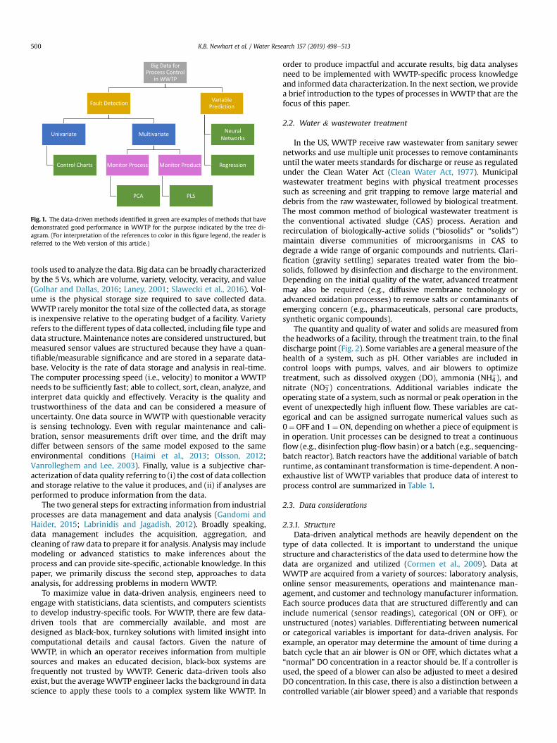
Fig. 1. The data-driven methods identified in green are examples of methods that havedemonstrated good performance in WWTP for the purpose indicated by the tree di-agram. (For interpretation of the references to color in this figure legend, the reader isreferred to the Web version of this article.)

K.B. Newhart et al. / Water Research 157 (2019) 498e513500

tools used to analyze the data. Big data can be broadly characterizedby the 5 Vs, which are volume, variety, velocity, veracity, and value(Golhar and Dallas, 2016; Laney, 2001; Slawecki et al., 2016). Vol-ume is the physical storage size required to save collected data.WWTP rarely monitor the total size of the collected data, as storageis inexpensive relative to the operating budget of a facility. Varietyrefers to the different types of data collected, including file type anddata structure. Maintenance notes are considered unstructured, butmeasured sensor values are structured because they have a quan-tifiable/measurable significance and are stored in a separate data-base. Velocity is the rate of data storage and analysis in real-time.The computer processing speed (i.e., velocity) to monitor a WWTPneeds to be sufficiently fast; able to collect, sort, clean, analyze, andinterpret data quickly and effectively. Veracity is the quality andtrustworthiness of the data and can be considered a measure ofuncertainty. One data source in WWTP with questionable veracityis sensing technology. Even with regular maintenance and cali-bration, sensor measurements drift over time, and the drift maydiffer between sensors of the same model exposed to the sameenvironmental conditions (Haimi et al., 2013; Olsson, 2012;Vanrolleghem and Lee, 2003). Finally, value is a subjective char-acterization of data quality referring to (i) the cost of data collectionand storage relative to the value it produces, and (ii) if analyses areperformed to produce information from the data.

The two general steps for extracting information from industrialprocesses are data management and data analysis (Gandomi andHaider, 2015; Labrinidis and Jagadish, 2012). Broadly speaking,data management includes the acquisition, aggregation, andcleaning of raw data to prepare it for analysis. Analysis may includemodeling or advanced statistics to make inferences about theprocess and can provide site-specific, actionable knowledge. In thispaper, we primarily discuss the second step, approaches to dataanalysis, for addressing problems in modern WWTP.

To maximize value in data-driven analysis, engineers need toengage with statisticians, data scientists, and computers scientiststo develop industry-specific tools. For WWTP, there are few data-driven tools that are commercially available, and most aredesigned as black-box, turnkey solutions with limited insight intocomputational details and causal factors. Given the nature ofWWTP, in which an operator receives information from multiplesources and makes an educated decision, black-box systems arefrequently not trusted by WWTP. Generic data-driven tools alsoexist, but the averageWWTP engineer lacks the background in datascience to apply these tools to a complex system like WWTP. In

order to produce impactful and accurate results, big data analysesneed to be implemented with WWTP-specific process knowledgeand informed data characterization. In the next section, we providea brief introduction to the types of processes in WWTP that are thefocus of this paper.

2.2. Water & wastewater treatment

In the US, WWTP receive raw wastewater from sanitary sewernetworks and use multiple unit processes to remove contaminantsuntil the water meets standards for discharge or reuse as regulatedunder the Clean Water Act (Clean Water Act, 1977). Municipalwastewater treatment begins with physical treatment processessuch as screening and grit trapping to remove large material anddebris from the raw wastewater, followed by biological treatment.The most common method of biological wastewater treatment isthe conventional activated sludge (CAS) process. Aeration andrecirculation of biologically-active solids (“biosolids” or “solids”)maintain diverse communities of microorganisms in CAS todegrade a wide range of organic compounds and nutrients. Clari-fication (gravity settling) separates treated water from the bio-solids, followed by disinfection and discharge to the environment.Depending on the initial quality of the water, advanced treatmentmay also be required (e.g., diffusive membrane technology oradvanced oxidation processes) to remove salts or contaminants ofemerging concern (e.g., pharmaceuticals, personal care products,synthetic organic compounds).

The quantity and quality of water and solids are measured fromthe headworks of a facility, through the treatment train, to the finaldischarge point (Fig. 2). Some variables are a general measure of thehealth of a system, such as pH. Other variables are included incontrol loops with pumps, valves, and air blowers to optimizetreatment, such as dissolved oxygen (DO), ammonia (NH4

þ), andnitrate (NO3

�) concentrations. Additional variables indicate theoperating state of a system, such as normal or peak operation in theevent of unexpectedly high influent flow. These variables are cat-egorical and can be assigned surrogate numerical values such as0¼OFF and 1¼ON, depending on whether a piece of equipment isin operation. Unit processes can be designed to treat a continuousflow (e.g., disinfection plug-flow basin) or a batch (e.g., sequencing-batch reactor). Batch reactors have the additional variable of batchruntime, as contaminant transformation is time-dependent. A non-exhaustive list of WWTP variables that produce data of interest toprocess control are summarized in Table 1.

2.3. Data considerations

2.3.1. StructureData-driven analytical methods are heavily dependent on the

type of data collected. It is important to understand the uniquestructure and characteristics of the data used to determine how thedata are organized and utilized (Cormen et al., 2009). Data atWWTP are acquired from a variety of sources: laboratory analysis,online sensor measurements, operations and maintenance man-agement, and customer and technology manufacturer information.Each source produces data that are structured differently and caninclude numerical (sensor readings), categorical (ON or OFF), orunstructured (notes) variables. Differentiating between numericalor categorical variables is important for data-driven analysis. Forexample, an operator may determine the amount of time during abatch cycle that an air blower is ON or OFF, which dictates what a“normal” DO concentration in a reactor should be. If a controller isused, the speed of a blower can also be adjusted to meet a desiredDO concentration. In this case, there is also a distinction between acontrolled variable (air blower speed) and a variable that responds

Fig. 2. A generic flow and sensor schematic of a CAS WWTP. Si denotes concentration of aqueous species i and is measured using offline laboratory analysis. Qi denotes the flowrateof either air, water, or supplemental carbon, which is measured using in-line flowmeters. DO, nitrate (NO3

�), and ammonia (NH4þ) are measured using sensors throughout the CAS

process to evaluate treatment performance, and at some facilities nutrient measurements are used to control the rate of biosolid recycle.

Table 1Examples of monitored features in WWTP and their associated data collection frequency and data structure.

Feature Frequency Structure Example

Water quality Daily-Monthly-Quarterly Numeric Laboratory analysis: 5-day biochemical oxygen demand, alkalinity, nutrientsWater quality Second-Minute Numeric Temperature, dissolved oxygen, pH, and nutrient concentrations from sensorsEquipment monitoring Second-Minute Categorical Power state, valve positionEquipment monitoring Second-Minute Numeric Operating speed, flowrate, pressureOperating setpoints Second-Minute Categorical Peak or normal operation for flow through, production or backwash for filtersOperating setpoints Second-Minute Numeric Runtime for batch operations

Table 2Examples of features with typically slow or rapid changes over time in a WWTP.

Timescale Feature

Slow (days-weeks) Solids retention time (SRT)Hydraulic retention time (HRT)Transmembrane pressure (TMP)

Fast (seconds-minutes) Dissolved oxygen (DO)Nutrient concentrationsTurbidityConductivityFlowrate


to the control (DO concentration). By measuring the effect ofexplanatory variables (i.e., control variables or other covariates) onresponse variables, data-driven methods can be developed to pre-dict the outcome of a process. However, not all analyses differen-tiate between explanatory and response. Additionally, not allexplanatory variables directly or measurably affect a processoutput, especially in a large process scheme like WWTP. Methodsapplied solely to explanatory variables are generally referred to asunsupervised, meaning that the goal is simply to identify patterns inthe data without any advance knowledge of the relationships beingsought. On the other hand, supervised learning occurs when theobservations are “labelled” by their response values, and the goal isto characterize the link between the explanatory and responsevariables. When a distinction between variable types is required, itis mentioned in the first instance of the method in Section 3.

2.3.2. Frequency and temporal variabilityWWTP data are collected at a variety of time intervals, from

continuous online sensor measurements to quarterly laboratoryresults. For example, WWTPmonitoring is considered “continuous”if data are collected at 15-min intervals or less (US EPA, 2015), butsome effluent quality variables are measured only every fewmonths, such as disinfection byproducts. Traditional data man-agement segregates data by source, primarily due to the difficultyof merging data of different frequencies and formats. A commonmathematical approach to handle different data frequencies is toscale data to a single time interval (Odom et al., 2018). However,datasets with a very large difference in frequencies cannot use thismethod because WWTP data are time-dependent, co-correlated(i.e., the relationships among variables are related to one another),and nonlinearly related, making downscaling challenging. Effluentquality variables may change either suddenly or gradually overtime (Table 2), and they often change nonlinearly in relation toother process variables, which can make attributing the cause ofchange between sampling events difficult.

The monitoring frequency of the treatment process strongly

depends on the goal of the analysis and the characteristics of theprocess (Venkatasubramanian, 1995). In process control, the datacollection frequency should be sufficiently high to account for in-strument noise and to track typical irregularities, but not sofrequent that excessive computational power is required for fullanalysis. Short-term faults, like a clog in a pipe that can occur on theorder ofminutes to hours, require a differentmonitoringwindowoftime than long-term faults like an increase in transmembranepressure due to biological fouling of a membrane that occurs on theorder of days to weeks (Table 2). Dürrenmatt and Gujer (2012)recommend a window width of at least three times the length oftime over which the fault occurs to be detected.

2.3.3. Variable characteristicsMany WWTP process variables exhibit unique characteristics

such as time-dependence and nonstationarity (e.g., the strongdiurnal and seasonal swings of ambient temperature), but con-ventional control strategies rarely account for such relationshipsthat need to be considered for data-driven fault detection, variableprediction, or automated control. Stationary variables have con-stant mean, variance, and covariances, making them predictableand more easily modeled. Conversely, the means and/or variancesof nonstationary variables change over time. If a variable's mea-surements are correlated from one time step to the next, the


variable is said to be dependent over time. WWTP data exhibitthese properties because of the dynamic nature of WWTP pro-cesses (Fig. 3); a constantly changing influent, batch as opposed tocontinuous processes, temperature, internal shifts in microbialecology, and process control instability are a few causes of thenonstationarity and temporal dependence.

Many statistical methods assume data are normally distributed.A normal distribution is symmetric, unimodal, and bell-shaped andis characterized by two statistical parameters, its mean and vari-ance. The multivariate case is additionally characterized by its co-variances (i.e., the variance between each pair of variables). Whenthe data are normally distributed, exact inferences can be madeabout the mean, variance, and covariances (e.g., confidence in-tervals, predictions, or hypothesis tests) because the distribution ofthe test statistics adhere to proven mathematical theories. Whenthe assumption of normality is not met, it is more difficult toidentify the distribution of the statistic. Without making assump-tions about the data's distribution, the uncertainty in the estimateof interest cannot be accurately inferred.

The assumption of normality does not typically hold in WWTP,due to boundary limits of variables (i.e., sensor operating range),process variation, and outliers. In the event of a hardware mal-function, a contaminated lab sample, or a data entry error, obser-vations may be missing or abnormal, compromising normality,analysis power, and reliability of results (Kwak and Kim, 2017). Eacherror can potentially bias features that are of interest to model, andthe removal or correction of erroneous values (i.e., data cleaning)should be a high priority prior to data analysis to limit incorrectconclusions (Haimi et al., 2013; Kadlec et al., 2009).

Particular attention needs to be paid to how a data-drivenmethodology is implemented. In the event that nonlinear andnonstationary behavior is detected, there are two approaches formodeling nonstationary behavior: accounting for a known, orpredictable, underlying trend or limiting the window of time overwhich a model is trained. Given the difficulty in modelingnonstationary behavior in WWTP (Fig. 3), relatively short windowsof time (e.g., 3 to 10 days) may be the best option to achieve

Fig. 3. Example of stationary and nonstationary process variables in WWTP. Membrane bioreand variance while permeate turbidity (top right), permeate conductivity (bottom left), an

approximate stationary and normal behavior.In addition to simple modifications of existing methods (e.g.,

using short training windows), distribution-free statisticalmethods, such as kernel density estimation (KDE) and boot-strapping, can be applied. KDE estimates a distribution using localsmoothing, allowing practitioners to work around the normalityassumption. However, KDE is very sensitive to the choice of tuningparameters (Izenman, 2013). Conversely, bootstrapping does notrequire any tuning parameters but is more computationallydemanding. From a dataset, observations are randomly drawnwithreplacement; the statistic of interest is computed; and then thesetwo steps are repeated many times to produce a distribution of thestatistic (Efron and Tibshirani, 1994). James et al. (2013) provide asimple introduction to the bootstrap method.

2.4. Exploratory data analysis

Identifying the structure and characteristics of a dataset requiresfamiliarity with the source of the data and the process itself. Plot-ting and visualizing data should be the first step in any analysis, butno one-size-fits-all approach exists. Observations recorded overtime can be visualized in time series plots (Fig. 3); the strength ofthe temporal dependence can be assessed with autocorrelationfunction plots; potential outliers can be observed in boxplots; andthe entire distribution can be plotted in a histogram. These plotswork well for monitoring a single variable, but WWTP are ofteninterested in the relationships among multiple variables. Pairwisescatterplots, multiple boxplots, functional boxplots, and cross-correlation function plots are just a few ways additional featurescan be assessed; examples of some of these plots can be found inPfluger et al. (2018). There are many tests available to assessmultivariate normality, including the Mardia test, Henze-Zirklertest, Royston test, Doornik-Hansen test, and the E-statistic(Korkmaz et al., 2014). Unsupervised learning methods for clus-tering or outlier detection are commonly used to identify structurein the data (James et al., 2013). Manual data inspection can be time-intensive, so the inclusion of more advanced statistical tools can

actor (MBR) tank level (top left) is considered a stationary variable with constant meand bioreactor (BR) DO concentration (bottom right) are nonstationary.


provide rapid insight into the data characteristics.

3. Methods & examples

In this section, we present the current use of process data inWWTP and a review of recent academic literature demonstratingthe possibilities for advanced, data-driven process control inWWTP. The focus of this review is on control methods that havebeen tested on actual WWTP systems to provide practitioners withrealistic examples. Simulation studies serve a valuable purpose butdo not always represent the WWTP process realistically due tosimplifying assumptions about data characteristics and the pro-cesses (Corominas et al., 2018). Primarily, data-driven analysis inWWTP can be used for fault detection, variable prediction, andautomated control. Each requires a different and increasinglycomplex data processing, analysis, and control framework. Thedata-driven methods are therefore discussed in the context of thegoal of each process control application: fault detection, variableprediction, or advanced control. We begin with a brief review ofhistorical methods of process control in WWTP.

3.1. Historical process control

Data-driven process control has historically been sparse inWWTP, with daily operational decisions considered more of an artthan a science (Metcalf and Eddy, 2013; O'Day, 2004). As early asthe 1920s, statistical tools like histograms and control charts wereused for informal diagnostics. Control during this time relied onmanual adjustments and observations, as digital control was not anoption prior to the 1960s. The cost of computers and instrumen-tation was high; treatment dynamics were not well understood;facilities were not designed with additional flexibility; and controltheory was not sufficiently developed (Olsson, 2012). In the 1980s,affordable computing power facilitated simple first principlemodels, although their complexity and lack of reliability madethem poor advisory systems (Olsson et al., 1998). By the early 2000sthe digital revolution reached WWTP, and most WWTP had inte-grated their own version of direct digital control into processmonitoring in the form of programmable logic controllers (PLC) andsupervisory control and data acquisition (SCADA) systems.

Despite the unique challenges posed by WWTP data, data-driven system automation and real-time control are integral tomodern WWTP operation. The most common process controlpractice is to maintain a set-point (i.e., target value) using onlinesensor readings and feedback control. For example, DO concen-trations can be controlled by adjusting air blower speed (i.e.,aeration intensity). Rather than operating at a single blower speed,online measurements provide feedback to the SCADA system thatdetermines whether blower speed should increase, decrease, orstay constant relative to a measured value, like DO concentration.Chemical dosing to enhance contaminant precipitation and addi-tional carbon for biological processes are other examples of feed-back control based on in-situ nutrient concentrations. This methodof process control is commonly achieved by a controller with avariable frequency drive to change operating conditions in acontinuous, smooth, and automated manner.

Establishing target values for process variables is one of thesimplest methods of control and is awidespread practice inWWTP.This single-variablemonitoring paradigm is the foundation for faultdetection at most modern WWTP, in which a measured value iseither within or outside of an operator-specified range. While thisapproach has a low false-alarm rate (e.g., if a flow rate measure-ment is below a set-point, a fault of unknown cause has certainlyoccurred somewhere in the system that affects flow rate), it can bevery slow to detect faults, does not forecast future values, and does

not account for correlations among variables. Plant operators mustbe available to respond quickly to a system fault to preventequipment damage or system failure, putting additional stress onequipment and staff to reduce a fault's impact on effluent waterquality. Proactive and comprehensive approaches to fault detectionand forecasting are being developed (Capizzi and Masarotto, 2017;Jiang et al., 2012; Kazor et al., 2016; Odom et al., 2018; Wang andJiang, 2009), which could help reduce cost and improve efficiencyof WWTP systems. Some data-driven fault detection methods arecurrently being implemented, and the results are discussed in thenext section.

3.2. Fault detection

A multitude of system faults or changes in conditions can causeprocess irregularities in WWTP. These include a change in influentquality (e.g., snowmelt, industrial discharge), an outbreak of mi-croorganisms that inhibit treatment (e.g., filamentous bacteria,algae), irregularities or damage to treatment units (e.g., mem-branes, clarifiers), mechanical failures (e.g., pumps, air blowers), orsensor failure (e.g., drift, bias, electrical interference). Each type offault can alter system performance differently, and it is importantto consider the versatility of an analytical approach (i.e., whichtypes of faults can be detected) when designing a fault detectionprogram. For example, if a sensor failure occurs and the sensor'smeasurements are included in a control loop, many variables couldbe affected. In contrast, if the sensor's measurements are notincluded in a control loop, a sensor fault may only affect themeasured sensor variable.

A “fault” is an unintentional deviation of a process characteristicthat limits the process’ ability to achieve its purpose (Isermann,1984). Typical single-variable faults that occur in WWTP areeasier to diagnose qualitatively and are illustrated in Table 3.However, multivariate faults can be much more difficult to discernvisually. To detect faults in the dynamic, nonstationary, multivar-iate data found in WWTP, a quantitative approach, such as statis-tical process control (SPC), is needed. In SPC, a “fault” is identifiedwhen a consecutive series of observations are flagged as abnormal.

Olsson and Newell (1999) suggested data collection frequencybe chosen to be at least one-fifth of the length of time over whichthe event of interest occurs. The distinction between normal (in-control or IC) and abnormal (out-of-control or OC) observations isdetermined by a statistical hypothesis test. Hypothesis tests areused to quantify the likelihood that an individual observation froma dataset is consistent with observations collected under IC con-ditions. IC observations are usually used to “train” an SPC model,which is a type of supervised learning because the initial data areknown to be IC. Many SPC methods exist, but few have beenimplemented in WWTP. The following is a discussion of differentSPC methods used in WWTP to determine if a significant change orfault has occurred.

3.2.1. Control chartsControl charts are useful tools to determine, at a glance, if a

process is IC. Themost popular statistical control chart was outlinedby Walter Shewhart of Bell Labs. The Shewhart control chart usesupper and lower control limits (UCL and LCL) for a process variableor statistic by adding or subtracting k standard deviations from thevariable's mean, with k¼ 3 being the industry standard (NIST/SEMATECH, 2003; Shewhart, 1926). If an observation is above theUCL (or conversely below the LCL), a statistically significant changehas most likely occurred. Shewhart control charts employed atWWTP are typically constructed with a 3- or 5-day arithmeticmoving average for variables designed to be stationary such assolids retention time (SRT) in a bioreactor or percent water

Table 3Abnormal patterns in univariate WWTP data that could indicate a fault and potential causes of the fault pattern. Adapted from Capizziand Masarotto (2017).

Pattern Cause

Isolated Power spike, air bubble on sensor, spike of contaminant in influent

Sustained Change in operational status, mechanical performance variation, sensor recalibration

Transient State change, sensor malfunction, cycle fluctuation

Drift Sensor or mechanical device degradation, biological shift, fluid flow restriction


recovery of a membrane treatment unit. Additionally, controlcharts can be used in WWTP analytical labs for quality control (e.g.,a sensor's measurements of a standard solution over time) (Riceet al., 2017) or other variables that change slowly (Table 2). How-ever, the Shewhart method of calculating control limits is only validfor a variable that is normally distributed and whose observationsare independent and stationary (Montgomery, 2009).

Updating the UCL and LCL to adapt to changing conditions usingmethods such as exponentially weighted moving average (EWMA)can account for some nonstationarity found in WWTP data (Wold,1994). The Shewhart control chart assumes the process is station-ary and weighs all past observations equally, ignoring trends(Montgomery, 2009). The EWMA gives more weight to the mostrecent observations, adapting to some process variation (NIST/SEMATECH, 2003) and is frequently used as a data smoothingtechnique (Berthouex and Box, 1996; Mina and Verde, 2007). TheEWMA accounts for both the most recent observation and pastbehavior bymultiplying themost recent observation by a forgettingfactor (0.05� l� 0.25) and the geometric moving average by 1 e l(Hunter, 1986; Montgomery, 2009; Roberts, 1959). However, theEWMA is not a good measure to distinguish between IC and OC forevery WWTP process. Like many data-driven performance moni-toring methods, the EWMA control limits are heavily impacted byoutliers (Rosen et al., 2003). In both panels of Fig. 4, the assimilationof OC observations immediately widens the range of values that areconsidered IC. Thus, control chart limits should only be updatedwith IC observations, as explored by Corominas et al. (2011).Additionally, some sensors have a lower operating limit, whichinvalidates the standard EWMA LCL (Fig. 4a). In this case, a turbiditysensor outputs a current between 4 and 20mA which is convertedto turbidity units (NTUs) using a calibrated linear regression. Here,4mA correlates to 0.04 NTU. When the turbidity is below thisthreshold, the sensor continues to output 4mA, which truncatesthe distribution of the turbidity data and invalidates the LCL. Forsmall datasets (e.g., fewer than two variables in the case of flow andpressure of a water distribution system), univariate EWMA hasshown to be better at detecting faults than multivariate EWMA(MEWMA) (Jung et al., 2013). However, most WWTP process vari-ables violate the assumptions required for the Shewhart's or theEWMA control chart (Berthouex, 1989), resulting in a high per-centage of false alarms, making them poor choices for fault detec-tion. For larger datasets (e.g., monitoring more than 2 processvariables), multivariate control charts can reduce a complicateddataset to a single measurement reflecting the “health” of theWWTP.

Monitoring multivariate processes (as opposed to individual

variable monitoring) with a control chart method may provideWWTP operators with a better sense of the overall state of oper-ating conditions (Schraa et al., 2006). Multivariate process statisticssuch as MEWMA (Lowry et al., 1992), multivariate cumulative sum(MCUSUM) (Crosier, 1988), and Hotelling's T2 (Hotelling, 1947) canbe used to examine the mean and dispersion of multiple variablesbut have rarely been implemented in industrial process monitoringdue to the complex matrix algebra required (NIST/SEMATECH,2003). MEWMA and MCUSUM have been shown to be good atdetecting small changes in the mean, compared to Hotelling's T2,but can have a high false-alarm rate (Alves et al., 2013). However,the assumption of multivariate normality is also required for thesemethods, and as mentioned previously, this is rarely observed inWWTP. A nonparametric approach, such as bootstrapping, mayyield better results for a multivariate control chart in WWTP(Phaladiganon et al., 2011).

3.2.2. Principal component analysisA widely used statistical method for monitoring multiple vari-

ables simultaneously is to capture the relationships among linearcombinations of variables rather than the variables themselves byprincipal component analysis (PCA) (Jackson, 1991). PCA identifiesindependent, linear combinations of variables (principal compo-nents or PCs) by effectively calculating lines-of-best-fit through adataset (Wise and Gallagher, 1996). PCs account for as much vari-ation as possible (given the assumption of linearity) and can,therefore, reduce the number of model variables and eliminatenoise and redundancy. For example, unsupervised PCA is frequentlyused to reduce the number of predictor (input) variables for mul-tiple regression models (discussed further in Section 3.3.3)(Wallace et al., 2016; Wang et al., 2017) and can be used to identify“clusters” of related microbiological sample properties (Jałowieckiet al., 2016).

To use PCA for supervised, data-driven analysis, a “training”dataset that represents IC conditions is used to calculate the PC,then “testing” data are transformed into the model subspace(defined by the PC). If the overall distance from a new observationto the PCA-model is above a desired control limit (similar to thecontrol chart methodology described above), then the new obser-vation is considered abnormal and is a possible indication of aprocess fault. The benefit of performing PCA prior to calculating thecontrol statistic (e.g., squared prediction error (SPE), Hotelling's T2,etc.) is the reduction in false alarms due to the reduction in noiseand removal of dependence among the features.

PCA has many applications inWWTP, from direct fault detection(King et al., 2006) to data reconstruction (Lee et al., 2006a; Schraa

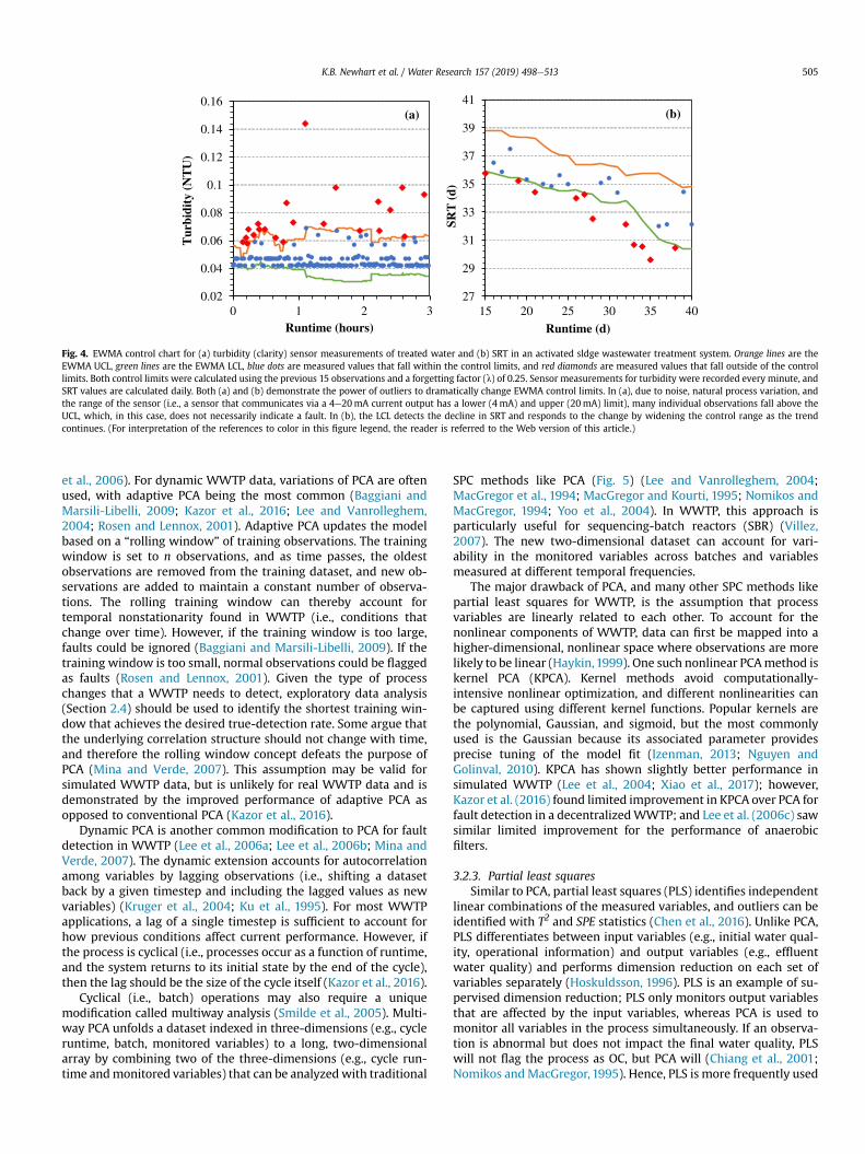
Fig. 4. EWMA control chart for (a) turbidity (clarity) sensor measurements of treated water and (b) SRT in an activated sldge wastewater treatment system. Orange lines are theEWMA UCL, green lines are the EWMA LCL, blue dots are measured values that fall within the control limits, and red diamonds are measured values that fall outside of the controllimits. Both control limits were calculated using the previous 15 observations and a forgetting factor (l) of 0.25. Sensor measurements for turbidity were recorded every minute, andSRT values are calculated daily. Both (a) and (b) demonstrate the power of outliers to dramatically change EWMA control limits. In (a), due to noise, natural process variation, andthe range of the sensor (i.e., a sensor that communicates via a 4e20mA current output has a lower (4mA) and upper (20mA) limit), many individual observations fall above theUCL, which, in this case, does not necessarily indicate a fault. In (b), the LCL detects the decline in SRT and responds to the change by widening the control range as the trendcontinues. (For interpretation of the references to color in this figure legend, the reader is referred to the Web version of this article.)


et al., 2006). For dynamic WWTP data, variations of PCA are oftenused, with adaptive PCA being the most common (Baggiani andMarsili-Libelli, 2009; Kazor et al., 2016; Lee and Vanrolleghem,2004; Rosen and Lennox, 2001). Adaptive PCA updates the modelbased on a “rolling window” of training observations. The trainingwindow is set to n observations, and as time passes, the oldestobservations are removed from the training dataset, and new ob-servations are added to maintain a constant number of observa-tions. The rolling training window can thereby account fortemporal nonstationarity found in WWTP (i.e., conditions thatchange over time). However, if the training window is too large,faults could be ignored (Baggiani and Marsili-Libelli, 2009). If thetraining window is too small, normal observations could be flaggedas faults (Rosen and Lennox, 2001). Given the type of processchanges that a WWTP needs to detect, exploratory data analysis(Section 2.4) should be used to identify the shortest training win-dow that achieves the desired true-detection rate. Some argue thatthe underlying correlation structure should not change with time,and therefore the rolling window concept defeats the purpose ofPCA (Mina and Verde, 2007). This assumption may be valid forsimulated WWTP data, but is unlikely for real WWTP data and isdemonstrated by the improved performance of adaptive PCA asopposed to conventional PCA (Kazor et al., 2016).

Dynamic PCA is another common modification to PCA for faultdetection in WWTP (Lee et al., 2006a; Lee et al., 2006b; Mina andVerde, 2007). The dynamic extension accounts for autocorrelationamong variables by lagging observations (i.e., shifting a datasetback by a given timestep and including the lagged values as newvariables) (Kruger et al., 2004; Ku et al., 1995). For most WWTPapplications, a lag of a single timestep is sufficient to account forhow previous conditions affect current performance. However, ifthe process is cyclical (i.e., processes occur as a function of runtime,and the system returns to its initial state by the end of the cycle),then the lag should be the size of the cycle itself (Kazor et al., 2016).

Cyclical (i.e., batch) operations may also require a uniquemodification called multiway analysis (Smilde et al., 2005). Multi-way PCA unfolds a dataset indexed in three-dimensions (e.g., cycleruntime, batch, monitored variables) to a long, two-dimensionalarray by combining two of the three-dimensions (e.g., cycle run-time andmonitored variables) that can be analyzedwith traditional

SPC methods like PCA (Fig. 5) (Lee and Vanrolleghem, 2004;MacGregor et al., 1994; MacGregor and Kourti, 1995; Nomikos andMacGregor, 1994; Yoo et al., 2004). In WWTP, this approach isparticularly useful for sequencing-batch reactors (SBR) (Villez,2007). The new two-dimensional dataset can account for vari-ability in the monitored variables across batches and variablesmeasured at different temporal frequencies.

The major drawback of PCA, and many other SPC methods likepartial least squares for WWTP, is the assumption that processvariables are linearly related to each other. To account for thenonlinear components of WWTP, data can first be mapped into ahigher-dimensional, nonlinear space where observations are morelikely to be linear (Haykin,1999). One such nonlinear PCAmethod iskernel PCA (KPCA). Kernel methods avoid computationally-intensive nonlinear optimization, and different nonlinearities canbe captured using different kernel functions. Popular kernels arethe polynomial, Gaussian, and sigmoid, but the most commonlyused is the Gaussian because its associated parameter providesprecise tuning of the model fit (Izenman, 2013; Nguyen andGolinval, 2010). KPCA has shown slightly better performance insimulated WWTP (Lee et al., 2004; Xiao et al., 2017); however,Kazor et al. (2016) found limited improvement in KPCA over PCA forfault detection in a decentralizedWWTP; and Lee et al. (2006c) sawsimilar limited improvement for the performance of anaerobicfilters.

3.2.3. Partial least squaresSimilar to PCA, partial least squares (PLS) identifies independent

linear combinations of the measured variables, and outliers can beidentified with T2 and SPE statistics (Chen et al., 2016). Unlike PCA,PLS differentiates between input variables (e.g., initial water qual-ity, operational information) and output variables (e.g., effluentwater quality) and performs dimension reduction on each set ofvariables separately (Hoskuldsson, 1996). PLS is an example of su-pervised dimension reduction; PLS only monitors output variablesthat are affected by the input variables, whereas PCA is used tomonitor all variables in the process simultaneously. If an observa-tion is abnormal but does not impact the final water quality, PLSwill not flag the process as OC, but PCA will (Chiang et al., 2001;Nomikos andMacGregor, 1995). Hence, PLS is more frequently used

Fig. 5. Visual representation of how multiway PCA unfolds a three-dimensional array into a two-dimensional matrix that can be analyzed with PCA. This particular configuration isconsidered “batch-wise” because the length of the batch is fixed. Another multiway unfolding could be “time-wise” if runtime is the same for each batch, and batches and variablesare merged.


in variable prediction than in fault detection.In complex systems, fault detection may improve by dividing

the process into units. Multiblock PLS (MB-PLS) subsets input var-iables into logical subsystems (e.g., primary sedimentation, aera-tion basin) prior to analysis (Wangen and Kowalski, 1989).Experimentally, MB-PLS does not improve prediction compared tothe standard PLS; however, the resultsmay be easier to interpret forfault diagnosis (Choi and Lee, 2005).

3.2.4. Neural networksConventional mechanistic models use complex formulas that

are connected in mathematically simple ways (i.e., mass balanceformulations to describe the sum of all unit processes). In contrast,neural networks (NN) use simple mathematical expressions thathave complex relationships inwhich process inputs are nonlinearlylinked to outputs without prior knowledge of an underlyingmechanism (Dreyfus, 2005; Nielsen, 2015; Olsson and Newell,1999). Process inputs and outputs are connected by “neurons”that are organized in layers (Fig. 6). A neuron in the input layerdistributes an actual process input variable to neurons in the firsthidden layer. Neurons in a hidden layer normalize and weighmultiple inputs, transform the value with an activation function,and produce a normalized output signal. NN can have one ormultiple hidden layers, connected by input transformations andoutput signals. The output layer is a weighted sum of the finalhidden layer's output signal.

In contrast to linear statistical models (e.g., multiple regression,PCA, PLS), NN model parameters do not have the same interpret-ability (i.e., no physical, chemical, or biological significance). Toidentify the parameters of each neuron in a NN model, learningalgorithms are needed. Due to the extensive intricacies of thedifferent learning algorithms for NN development, this paper willfocus on the two types of NN training: supervised or unsupervised.

Supervised training requires data to be labelled in such a way

Fig. 6. A generic neural network structure. NN can contain multiple hidden layers withdifferent numbers of neurons in each layer, and one hidden layer is shown here.

that inputs and outputs are defined. There are many differentlearning algorithms for fitting a supervised NN, and each requiresan iterative process in which parameters are estimated based on alarge historical dataset (Dreyfus, 2005). One of the most common isthe back-propagation learning algorithm that starts by randomlyassigning parameter values, calculating an estimated output, andminimizing the error between the estimated and the actual output,node by node and layer by layer, starting with the hidden layerdirectly connected to the output. Hundreds of iterations must beperformed to determine the best network for a particular dataset,requiring a substantial amount of computing power (Wei, 2013).Hence, it is valuable to minimize the number of variables used toconstruct the model.

Unsupervised training of a NN uses data that are unlabeled (i.e.,the model is supplied with defined inputs but no outputs) and usesfundamentally different learning algorithms than the error-correction method in supervised training. Unsupervised NN actbest as classifiers for pattern recognition. In fault detection, unsu-pervised NN can be trained to model a process by estimating thevalues of inputs and comparing the estimation to the actual values,also known as an auto-encoder NN (ANN). Xiao et al. (2017) usedANNs with “bottleneck” layers (i.e., the middle, hidden layer con-tains fewer nodes than the preceding or succeeding layers), whichforce the NN to effectively capture the principal components of thedata to detect faults at a WWTP. SPE was calculated from the dif-ference between actual and estimated values, and similar to PCA, anSPE threshold was calculated to determine if the process was IC orOC. Xiao et al. (2017) concluded that ANN-based fault detectionwasmore sensitive to changes than conventional PCA. Additionally,Xiao et al. (2017) compared “deep” and “shallow” ANN. Untilrecently, training NN with many layers and nodes (“deep” NN) wasnot computationally efficient (Hinton et al., 2006). However,“shallow” NN are generally unable to capture highly-nonlinearsystems. In this case, there was no conclusive evidence that thedeep ANN performed better than the shallow ANN.

3.3. Variable prediction

SPC can be used to assess if a system is IC or OC, but this is ageneric measure of product water quality and system health. Topredict what a variable value should be under given conditions,model-based control could be used. Model predictive control (MPC)compares mechanistic model predictions to actual process mea-surements. Then, deviations from the model are identified as faults.The model can be derived from theory (i.e., fluid dynamics, mi-crobial kinetics) or empirical trends (i.e., data-driven) and can beused to approximate additional process variables. In lieu of directly


monitoring the variable of interest, a link may be found amongvariables. In this way, a software sensor or “soft sensor” (alsoreferred to as inferential sensors, virtual online analyzers, orobserver-based sensors) can be developed for the online moni-toring of variables that are too time-consuming or expensive toconsistently monitor with lab-based analyses (Ch�eruy,1997; Kadlecet al., 2009). Many different approaches to variable prediction havebeen proposed, and here we review the most commonly observedin literature.

3.3.1. Activated sludge modelsSome water quality variables can be adequately predicted with

calibrated, first-principal models. The activated sludge model no. 1(ASM1) is the most widely used deterministic model for biologicalcarbon and nitrogen removal in WWTP (Henze et al., 1987). ASM1was developed in 1985 by compiling novel research about the ki-netic behavior andmechanisms of the CAS process. Subsequent CASmodels (e.g., ASM2 and ASM2d) have additional parameters thataccount for fermentation, enhanced biological phosphorusremoval, and chemical phosphorus removal (Gujer et al., 1999;Henze et al., 1999, 1995). Models based on first principals also existfor clarifiers/settlers, but due to a lack of a mathematical relation-ship between floc characteristics and settleability, they are stilllimited to process design and research purposes (Metcalf and Eddy,2013; Olsson, 2012). Uncertainty in the model inputs and thesimplified mathematical framework fundamentally limits the ac-curacy of the model. However, in many cases, pilot- or full-scalecalibration can account for some of the error in the ASM (Metcalfand Eddy, 2013). Additional sources of error are model parameterestimates. Not all unit processes share a common set of state var-iables (i.e., variables that indicate the operating conditions of aprocess as opposed to variables that measure a constituent in thewater), and linking models with variable estimates can lead tosubstantial error in the plant-wide model (Volcke et al., 2006). Forexample, ASM and secondary clarifier models are frequentlycoupled, but the models differ in how total suspended solids (TSS)concentration is calculated and incorporated.

Without calibration and only parameter estimates, the ASMmayproduce results that are only accurate within an order of magni-tude, illustrating the variability of WWTP (Gujer, 2011). Olsson andNewell (1999) considered other sources of error for model pre-dictions, including inaccurate or incorrect calibration, non-idealprocess behavior, and lump-sum parameter assumptions. Forthese reasons, MPC with the ASM is rarely used in full-scale bio-logical WWTP operations for variable prediction or fault detection.

To standardize control strategy testing at biological WWTP, asimulation benchmark was developed from the ASM1 (Henze et al.,1987) under EU COST Actions 682 and 624 (Alex et al., 1999;Jeppsson and Pons, 2004; Spanjers et al., 1998). The BenchmarkSimulation Model No.1 (BSM1) includes a mathematical model of afive-reactor CAS treatment system followed by a clarifier (Fig. 2),ASM-specific parameters from literature, and simulated influentdatasets for different weather events (Copp, 2002). The newestversion, BSM2, incorporates extensions proposed in recent litera-ture: a longer simulation study timeframe, inclusion of temporallydynamic parameters, andmore realistic sensor behavior and failure(Jeppsson et al., 2007; Nopens et al., 2010; Rosen et al., 2004).

There are hundreds of proposed control strategies for the BSM,but simulation benchmarks do not yet exist for all commonwastewater treatment technologies. While simulation studies areimportant to understand the potential behaviors of control strate-gies, the actual dynamics of a WWTP are nearly impossible toreproduce artificially. This is most evident when control strategiesperform well on BSM but cannot be replicated with real WWTPdata (Sin et al., 2006). Oppong et al. (2013) compared simulated

datasets from the BSM models to real industrial WWTP data usinganaerobic digestion in an attempt to develop a soft sensor. How-ever, the variable of interest (volatile solids concentration) hadsubstantially different co-correlation structure, both in magnitudeand direction, among the simulated and actual process variables.The difference was attributed to infrequent sampling and a stableprocess with little change, but it is also possible that the BSM isinadequate for MPC in this case.

3.3.2. Transfer function modelsTransfer function models are a general class of models that

describe the relationship between an input and output of a linearsystem using a mathematical function. When the system is not toocomplex (i.e., the number of output parameters is� 2), transferfunctions can be a good approximation for dynamic systems (Boxet al., 1994). Univariate autoregressive integrated moving average(ARIMA) models are a special case of transfer function models thatdo not depend on the input variables and are widely used for lineartime series forecasting (Chen et al., 2007). The autoregressive (AR)portion predicts values that are mathematically related to theprevious time-step(s) (i.e., lag). The moving average (MA) predictsvalues that are mathematically related to the error of the past time-steps. The integrated (I) portion of the ARIMA model indicates thatthe difference between observations (one or more) is modeledinstead of the observation itself, and this step can remove some ofthe nonstationarity present in the data.

The primary application of ARIMAmodels inWWTP is to predictan effluent variable. Park and Koo (2015) showed that an ARIMAmodel can be used to predict effluent turbidity of a sedimentationbasin. Berthouex and Box (1996) andWest et al. (2002) successfullyused an ARIMAmodel to predict effluent 5-day biochemical oxygendemand (BOD5) of a WWTP. However, the ARIMA model's inte-gration step is often insufficient to account for WWTP data non-stationarity in the long-term (West et al., 2002). As the predictionhorizon increases, the accuracy of ARIMA models declines sub-stantially; unable to account for nonlinear behavior in WWTP(Dellana and West, 2009).

3.3.3. Multiple regressionMultiple regression is an extension of a simple, linear regres-

sion, using multiple independent variables (Xi, i¼ 1, 2, …, k) tomodel a single dependent variable, Y, via Y¼ b0 þ b1X1 þ … þbkXkþe. The model parameters are commonly estimated by ordi-nary least squares, andmore information about multiple regressionmodel fitting can be found in Sheather (2009). When all indepen-dent variables are standardized (i.e., zero mean and unit variance),the strength of an input variable's impact on the output variable isdirectly proportional to the magnitude of bi, giving tangiblemeaning to the model parameters. Categorical information can alsobe integrated by the use of dummy variables (Di, i¼ 1, 2, …, k),which take on binary values (e.g., if a blower is ON, then Di¼ 1; ifOFF, then Di¼ 0). However, problems can arise when fitting amultiple regression model if the explanatory variables are exactlylinearly related (multicollinearity), are highly variable, or areautocorrelated (Miah, 2016) as in WWTP.

Ebrahimi et al. (2017) used multiple regression models to pre-dict various water quality variables like phosphorus, nitrogen, andTSS concentrations in a full-scale wastewater treatment plant withreasonable results (r2¼ 0.71e0.87, meaning the model explains71e87% of total variation in the dependent variable), but they didnot demonstrate sufficient accuracy for stand-alone fault detection.However, multiple regression techniques may have applications insoft sensor and empirical model development.

PLS regression is a combination of PLS and multiple regressionand can be used to predict the output variables from the input

Fig. 7. Simplified example of MPC. At time¼ 0 (the intersection of the axes), themeasured variable's setpoint is increased. The mechanistic model and a functiondescribing the energy consumption of the control mechanism are used to identify theoptimum control response to reach the new setpoint over a given time interval (i.e.,prediction horizon).


(Abdi, 2003). Because of this property, PLS is commonly used forindustrial soft sensors and water quality variables in WWTP, suchas chemical oxygen demand (COD), TSS, nitrate, and oil and greaseconcentrations (Langergraber et al., 2003; Qin et al., 2012). The useof nonlinear mapping with PLS (kernel PLS or KPLS) also showspromise for methane production from a full-scale anaerobic filter(Lee et al., 2006c) and COD, total nitrogen, and cyanide concen-tration in CAS (Woo et al., 2009). In these cases, KPLS performedbetter than conventional PLS, which demonstrates the importanceof accounting for nonlinearities for some data-driven applications.

3.3.4. Neural networksSupervised NN have been used to predict raw wastewater flow

from online rainfall data and historical influent data (Wei, 2013).Yang et al. (2008) reconstructed COD concentration from UV-254and pH measurements using a back-propagation NN. €Omer Faruk(2009) used a hybrid NN-ARIMA to predict boron and DO concen-trations and water temperature of a river over time. While theARIMA model performed very poorly (r2¼ 0.23e0.55), the hybridmodel performed only slightly better (r2¼ 0.79e0.83) than the NNmodel (r2¼ 0.77e0.81). NN-ARIMA hybridization has been a pop-ular research topic because, in theory, both linear and nonlinearbehavior could be described with the resulting model(Venkatasubramanian, 1995). However, few case studies exist thatdemonstrate a significant improvement of a hybrid model over aNN model (Chen et al., 2007).

A NN hybrid model was successfully used by Lee et al. (2008) topredict COD, total nitrogen, and total phosphorus concentrations inthe effluent of small CAS WWTP from conductivity, temperature,pH, DO, oxidation-reduction potential (ORP), and turbidity. Inputand output variables were lagged to account for dynamic processvariation, combined with a transfer function model (auto-regres-sive representations with exogenous inputs or ARX). Lee et al.'s(2008) approach showed good results for variable prediction(r2¼ 0.92e0.95) and is promising for soft sensor development.

Lee et al. (2002) also used a hybrid NN structure for prediction ofWWTP effluent quality. In principle, the hybridization of mecha-nistic and NN models bridges the gap between first principal andstatistical approaches. The NN was placed in parallel and in serieswith the ASM1 model to estimate the model error or input pa-rameters, respectively. The parallel hybrid NN model performedwell at predicting effluent variables (e.g., cyanide r2¼ 0.93e0.96),but the series hybrid NN model did not perform better than the NNalone, indicating that there exists some error for which the ASM1model itself does not account.

Models to determine sorption kinetics and the capacity of car-bon to adsorb contaminants can also be mapped by NN. VasanthKumar et al. (2008) trained an NN model with batch experi-mental data under various conditions to predict equilibrium con-centrations after the uptake of dye by powdered activated carbon(PAC). The resulting predictions were nearly perfect (r2¼ 0.96).However, hundreds of data points were needed to calibrate themodel prior to the predictions; there was not significant variationamong the input variables; only a single contaminant was used;and separate testing data was not used to verify results. Given thecomplexity of biological treatment modeling, generating a carbonadsorption isotherm for PAC treatment is very well understood,computationally straightforward, and accurate for design purposes.Unless NN can demonstrate the ability to account for large varia-tions in initial water quality (of which the current isotherm para-digm cannot), use of the traditional adsorption isotherm modelswill continue to be used. A potential application that has not yetbeen explored is for the generation of isotherm models for micro-pollutants (e.g., per- and polyfluoroalkyl substances) in the pres-ence of bulk organic carbon.

3.4. Advanced control

The goal of WWTP optimization is to achieve the desiredeffluent quality with fewer inputs (i.e., chemicals, energy,manpower). Future WWTP will also need to be able to adjust theireffluent quality to meet new demands without risk of disturbance.As water resources dwindle and demand increases in urban cen-ters, customizable water quality based on need and time of year(known as “tailored” water) has become an attractive option(Vuono et al., 2013). Using historical data and system knowledge, afunction can be developed to minimize cost or energy whilemaintaining effluent quality in order to identify the best set ofsetpoints and control decisions. This is a fundamentally differentapproach than heuristically adjusting variable setpoints andobserving the system's response. Various methods to achieve data-driven control (“advanced or automated control”) are discussed inthis section. However, advanced control is still in its infancy forWWTP, and few full-scale demonstrations or installations exist.

3.4.1. Model predictive controlMPC uses a mechanistic model of a process to predict a process

variable accounting for the physical constraints of a system's actualprocess variable measurements (Richalet et al., 1978). The modelpredicts future process behavior over a time interval (known as theprediction horizon), and predictions are compared to online mea-surements to determine if a change has occurred (Fig. 7). MPC isless common in WWTP because most individual WWTP processes,especially biological processes, are too complex to develop suffi-ciently accurate first principal models (Section 3.3.1) for advancedcontrol purposes due to their deviation from ideal, steady-stateconditions (Patton et al., 2000). Furthermore, the computing po-wer required to handle the nonlinearities has not been welldocumented.

MPC in WWTP takes on many forms, but all must addressWWTP data's nonlinear behavior. Nonlinear models are computa-tionally intensive to solve, and accounting for too many non-linearities can substantially slow a controller's response. A lesscomputationally intensive option is to use piecewise linear MPC inwhich multiple linear models approximate a nonlinear model(Ocampo-Martinez, 2010; Olsson and Newell, 1999). Anothermethod is to update or adapt linear model parameters to fit currentoperating conditions (Zhang and Zhang, 2006). Adaptive MPCcontrollers have been shown to perform better than conventionalPID controllers for nonlinear processes; however, strong non-linearities are still better handled by alternative control approachessuch as NN (Hermansson and Syafiie, 2015).


MPC has been implemented for dynamically simplistic WWTPunit processes, such as membrane-based treatment, that can becontrolled by a single variable. Membrane systems can be easilymodeled using known relationships of fluid flow, mass transfer, andthermodynamics. Bartman et al. (2009) derived such a model tocontrol a valve on a pilot-scale reverse osmosis (RO) membranetreatment system. The reject (concentrate) flowrate was controlledby the dynamic, nonlinear, lumped-parameter model and wasvalidatedwith experimental data. In general, the system performedbetter when controlled by the dynamic model as opposed to atraditional controller.

Not all WWTP unit processes are fit for MPC simply becauseaccurate analytical models do not yet exist, and the number ofpossible inputs makes real-time control computationally unrea-sonable. Attempts have been made in the literature to adapt MPCfor WWTP, including CAS and membrane systems, but moreresearch is needed to develop realistic and system-specific modelsbefore MPC can be implemented as a control strategy in full-scaleWWTP. Alternatively, non-deterministic, nonlinear, data-drivenmodels are an option for MPC of activated sludge systems (i.e., NN).

3.4.2. Neural networksAs discussed in Section 3.3.4, each parameter and layer in an NN

model adds an additional degree of flexibility that can address theproblem of nonlinear model fitting. However, a large number of NNmodel parameters can risk overfitting to noise in the data ratherthan the process itself and can unnecessarily increase computation.The computational power required to use an NN model for controlapplications is not well documented, and most studies in WWTPliterature utilize only a few water quality variables to predict asingle value (i.e., soft sensor development). The availability ofreliable and plentiful online sensor data can also be a majorconstraint. More research is needed with constructing largerWWTP NN before the practicality of NN control strategies inWWTPcan be assessed. To begin, WWTP NN model development shouldbe performed incrementally, so that an unexpected and unman-ageable amount of computational power is not required to achieve

Fig. 8. Illustration of repeating patterns of ORP and pH data in parallel reactors of a batchindicate the completion of different stages in biological nitrogen removal. Adopted from D

simple goals.One proposed method of using NN in nonlinear dynamic pro-

cess control is to adjust the NN structure (i.e., number of hiddenneurons) and parameters (i.e., node weights) during the trainingphase, also referred to as an unsupervised, self-organizing NN. Ateach node, an optimization function determines if the node shouldbe deleted, kept the same, or split into two, and the node param-eters are adjusted accordingly. Post-training, self-organizing NNhave been shown to perform better (i.e., lower computation timeand testing error) than NNwhere the structure is fixed (i.e., numberof nodes) (Han et al., 2010). Han and Qiao (2014) used a self-organizing NN to model aeration and recirculation (i.e., DO andnitrate concentration) and a multiple-objective controller to opti-mize control of a pilot-scale CAS system. However, the authors didnot compare system performance to a conventional controller,making it difficult to justify implementation for the purpose of DOand nitrate concentration control, given computational re-quirements for real-time control of a larger system.

NN controllers are also being designed to detect nonlinear time-varying data features that indicate the end of a reaction, such asORP in CAS (Fig. 8). Luccarini et al. (2010) used an NN program tocontrol and optimize biological nitrogen removal for a pilot-scaleSBR. The end of denitrification (i.e., a biological process to removenitrate) could not be detected well due to a 50% historicalcompletion rate at the pilot facility. The end of nitrification isdifficult to detect because of noise and the small change in therising ORP and DO. The lack of detection, in this case, demonstratesa common drawback of many data-driven systemsdthe desiredperformance must be demonstrated consistently.

3.4.3. Transfer function modelsTransfer function models can be used for MPC and optimization

in addition to variable prediction discussed in Section 3.3.2. O'Brianet al. (2011) demonstrated the ability of a first-order, six variableARX MPC to optimize energy consumption by reducing aeration by25% at a full-scale CAS WWTP, compared to the facility's originalPLC-based control strategy. However, in this case, providing

activated sludge system. The ORP elbow, nitrate apex and knee, and ammonia valleyubber and Gray (2011).


aeration based on influent organic loading is not a novel concept,and much of the improvement can be attributed to a poorly cali-brated or performing controller.

3.4.4. Fuzzy logicIn diagnosing process upsets, multiple WWTP operators may

logically reach different conclusions regarding the cause of aproblem. Unlike computers, human decision-making is not alwayslogical, and choices are not always binary (i.e., true or false). Fuzzylogic mimics the attributes of human reasoning by “blurring” theinputs and rules to allow for “partial” truth. To achieve this, fuzzylogic uses linguistic variables in place of numerical variables, de-fines relationships among variables (“clustering”) with IF-THENstatements that allow for different degrees of truth, and charac-terizes the relationships by fuzzy algorithms. The seminal paperdescribing fuzzy logic by Zadeh (1973) is recommended for readersinterested in more details on fuzzy model structure.

The classic rule development approach for fuzzy models is towrite IF-THEN relationships explicitly, which is time-consuming forboth computer scientists andWWTP operators. This process can besimplified by using an NN to map operator observations into fuzzyrules. Enbutsu et al. (1993) re-structured the traditional NN modelwith fuzzy neurons in the input and output layers to model PACdosing and established rules that were more accurate than thosederived from interviews with water treatment operators.

Taw-Hwan et al. (1997) also used a hybrid fuzzy model-NNapproach, but calculated PAC-dosing rate with a fuzzy model un-der normal conditions and used an NN model when abnormalitieswere detected (i.e., turbidity >30 NTU). Jar-tests were used tocollect data to build both the fuzzy model and NN model, whichpredicted PAC-dosing rate very accurately during a one-year fieldtest at a full-scale water treatment plant.

Yoo et al. (2003) used PCA combined with fuzzy clustering and afuzzy model to predict COD removal from a full-scale industrialWWTP. PCA was used to reduce the complexity of the fuzzy modelas well as to reduce co-linearity. Results were able to generallypredict COD removal but could not be used for direct control,demonstrating that not all combinations of data-driven solutionsare always effective.

Bello et al. (2014) used fuzzy clustering to define rules for amulti-input, multi-output coagulant-dosing system in a watertreatment plant. The pH predictions were calculated from previouspH values and flowrates of three coagulants and coagulant-aids. Inthis case, fuzzy MPC performed slightly better than a nonlinearmodel approximated by linearization. If conditions were to changesubstantially over time (i.e., if the model parameters needed toadapt over time), fuzzy models may be a practical alternative tononlinear MPC.

4. Conclusions and recommendations

The future of data-driven and big data analytics in WWTP (andwater treatment) is in improving process control to reduce energydemand, ensure effluent water quality, and prevent system failure.To achieve this, WWTP need to incorporate data-driven faultdetection, variable prediction, and automation into their currentprocess control paradigms. Despite a large body of literature onmany data-driven process control methods in WWTP, there is noconsensus on a singular “best” approach. For fault detection anddiagnosis, WWTP need to understand past and present behavior interms of IC or OC.” Control charts are good for monitoring singlevariables that are measured daily to monthly and do not contain alot of noise (e.g., laboratory analysis, SRT). To evaluate multiplevariables for fault detection and diagnosis, PCA is good for use withcomposite samples because it does not distinguish between input

and output variables like PLS. To use big data in wastewater treat-ment to predict future performance, the monitored variable(s)must have a high sample frequency and number of historical ob-servations, but do not need to be linearly related or parametricallydistributed.

A small, decentralized facility may experience so much opera-tional variability that MPC is not effective; thus, SPC may beimplemented to detect faults and reduce the number or length oftime on-site operations staff must be present. For a large, central-ized facility with the buffering capacity to operate at quasi-steady-state (compared to the decentralized case), MPC may be useful forreducing chemical inputs and energy optimization. An additionalconsideration is the development of tools to optimize operations atthe unit process scale (e.g., aeration basin with recycling, mem-brane bioreactor) in addition to the plant-wide scale. Differenttasks will employ different problem-solving methodologies.Models that reveal more mechanistic information to assist withdiagnosis tend to have poor fault detection accuracy in highlynonlinear systems. Hence, a hybrid method combining model andstatistical process control may be a superior problem-solvingapproach. Each approach will come at a computational cost,which is rarely reported in the literature; with the major limitingfactor being the quality and quantity of data generated by WWTP.

To develop high-quality and accurate big data tools for waste-water treatment industry data scientists, computer scientists, andengineers must continue to collaborate to maximize data's poten-tial. The effectiveness of many state-of-the-art data science toolshave not yet been tested in WWTP. Random forests, support vectormachines, and reinforcement learning have the potential toaccommodate many of the features of WWTP data, but they stillrequire large training datasets to fit and must produce reliable re-sults (Kusiak et al., 2013; Verma et al., 2013). With WWTP opera-tions, transparency in methodology is one of the keys to adoption,so some advanced methodologies may continue to be eschewed infavor of simpler but interpretable methodologies.

In summary, WWTP looking to integrate data-driven controlshould:

1. Define the scope of the problem and desired goals.2. Identify which variables are currently being monitored (or

should be monitored) to effectively capture the scope of theproblem.

3. Use plotting tools to investigate the characteristics of each var-iable as well as the relationships between variables.

4. Based on the features observed in the data and analysis goals,identify the appropriate method to implement. Recommenda-tions for further reading on each broad category of methods aregiven throughout the text.

5. Fit the models and assess their validity. Visualize results toensure that the conclusions are logical and realistic.

6. Share the results with other WWTP via industry-specific pub-lications and conferences to develop mainstream, data-drivenprocess control tools for WWTP.

Acknowledgments

Support for this study was provided by the National ScienceFoundation Partnership for Innovation: Building Innovation Ca-pacity project 1632227 and by the National Science FoundationEngineering Research Center program under cooperative agree-ment EEC-1028968 (ReNUWIt). The authors would also like tothank Dr. Tanja Rauch-Williams and Dr. Eric Dickenson for theircomments on earlier drafts. The anonymous comments from threereviewers also greatly contributed to framing the content of thisreview.


Acronyms

ANN Auto-Encoder NNAR AutoregressiveARIMA Autoregressive integrated moving averageARX Auto-regressive representations with exogenous inputsASM Activated sludge modelBOD5 5-day biochemical oxygen demandBSM Benchmark simulation modelCAS Conventional activated sludgeCOD Chemical oxygen demandDO Dissolved oxygenEWMA Exponentially weighted moving averageIC In-controlKDE Kernel Density EstimationKPCA Kernel PCALCL Lower control limitsMCUSUM Multivariate Cumulative SumMA Moving averageMB-PLS Multiblock PLSMEWMA Multivariate EWMAMPC Model predictive controlNH4

þ AmmoniaNN Neural networksNO3

- NitrateNTU Nephelometric Turbidity UnitOC Out-of-controlORP Oxidation-reduction potentialPAC Powder activated carbonPCA Principal component analysisPLC Programmable logic controllersPLS Partial least squaresSBR Sequencing batch reactorsSCADA Supervisory control and data acquisitionSPC Statistical process controlSPE Squared prediction errorSRT Solids retention timeTSS Total suspended solidsUCL Upper control limitsWWTP Wastewater treatment plant

References

Abdi, H., 2003. Partial least squares (PLS) regression. In: Lewis-Beck, M.,Brayman, A., Liao, T.F. (Eds.), Encyclopedia of Social Sciences Research Methods.Sage, Thousand Oaks, CA.

Alex, J., Beteau, J.F., Copp, J.B., Hellinga, C., Jeppsson, U., Marsili-Libelli, S., Pons, M.N.,Spanjers, H., Vanhooren, H., 1999. Benchmark for Evaluating Control Strategiesin Wastewater Treatment Plants. European Union Control Association.

Alves, C., Henning, E., Samohyl, R., Cristina Konrath, A., Formigoni CarvalhoWalter, O., 2013. Application of multivariate control charts for monitoring anindustrial process. Tecno-L�og. 17, 101e107. https://doi.org/10.17058/tecnolog.v17i2.3636.

Baggiani, F., Marsili-Libelli, S., 2009. Real-time fault detection and isolation inbiological wastewater treatment plants. Water Sci. Technol. 60. https://doi.org/10.2166/wst.2009.723.

Bartman, A.R., Christofides, P.D., Cohen, Y., 2009. Nonlinear model-based control ofan experimental reverse-osmosis water desalination system. Ind. Eng. Chem.Res. 48, 6126e6136. https://doi.org/10.1021/ie900322x.

Bello, O., Hamam, Y., Djouani, K., 2014. Fuzzy dynamic modelling and predictivecontrol of a coagulation chemical dosing unit for water treatment plants.J. Electr. Syst. Inf. Technol. 1, 129e143. https://doi.org/10.1016/j.jesit.2014.08.001.

Berthouex, P.M., 1989. Constructing control charts for wastewater treatment plantoperation. J. Water Pollut. Control Fed. 61, 1534e1551.

Berthouex, P.M., Box, G.E., 1996. Time series models for forecasting wastewatertreatment plant performance. Water Res. 30, 1865e1875. https://doi.org/10.1016/0043-1354(96)00063-2.

Box, G.E.P., Jenkins, G.M., Reinsel, G.C., 1994. Time Series Analysis - Forecasting andControl, fourth ed. Wiley.

Capizzi, G., Masarotto, G., 2017. Phase I distribution-free analysis of multivariate

data. Technometrics 59, 484e495. https://doi.org/10.1080/00401706.2016.1272494.

Chen, A., Zhou, H., An, Y., Sun, W., 2016. PCA and PLS monitoring approaches forfault detection of wastewater treatment process. In: Presented at the 2016 IEEE25th International Symposium on Industrial Electronics (ISIE). https://doi.org/10.1109/ISIE.2016.7745032.

Chen, S.-H., Wang, P.P., Kuo, T.-W., 2007. Computational Intelligence in Economicsand Finance. Springer.

Ch�eruy, A., 1997. Software sensors in bioprocess engineering. J. Biotechnol. 52,193e199. https://doi.org/10.1016/S0168-1656(96)01644-6.

Chiang, L.H., Russell, E.L., Braatz, R.D., 2001. Fault Detection and Diagnosis in In-dustrial Systems.

Choi, S.W., Lee, I.-B., 2005. Multiblock PLS-based localized process diagnosis.J. Process Control 15, 295e306. In: https://doi.org/10.1016/j.jprocont.2004.06.010.

Clean Water Act, 1977.Copp, J.B., 2002. The COST Simulation Benchmark: Description and Simulator

Manual. European Cooperation in the field of Scientific and Technical Research(COST).

Cormen, T.H., Leiserson, C.E., Rivest, R.L., Stein, C., 2009. Introduction to Algorithms,third ed. The MIT Press.

Corominas, L., Garrido-Baserba, M., Villez, K., Olsson, G., Cort�es, U., Poch, M., 2018.Transforming data into knowledge for improved wastewater treatment oper-ation: a critical review of techniques. Environ. Model. Softw., Special Issue onEnvironmental Data Science. Applications to Air quality and Water cycle 106,89e103. https://doi.org/10.1016/j.envsoft.2017.11.023.

Corominas, L., Villez, K., Aguado, D., Rieger, L., Ros�en, C., Vanrolleghem, P.A., 2011.Performance evaluation of fault detection methods for wastewater treatmentprocesses. Biotechnol. Bioeng. 108, 333e344.

Crosier, R.B., 1988. Multivariate generalizations of cumulative sum quality-controlschemes. Technometrics 30, 291e303. https://doi.org/10.1080/00401706.1988.10488402.

Dellana, S.A., West, D., 2009. Predictive modeling for wastewater applications:linear and nonlinear approaches. Environ. Model. Softw 24, 96e106. https://doi.org/10.1016/j.envsoft.2008.06.002.

Diebold, F.X., 2003. Big data" dynamic factor models for macroeconomic mea-surement and forecasting. In: Dewatripont, M., Hansen, L.P., Turnovsky, S. (Eds.),Advances in Economics and Econometrics: Theory and Applications, EighthWorld Congress of the Econometric Society. Cambridge University Press,Cambridge, pp. 115e122.

Dreyfus, G., 2005. Neural networks: an overview. In: Neural Netw. SE - 1 1e83.https://doi.org/10.1007/3-540-28847-3_1.

Dubber, D., Gray, N.F., 2011. The effect of anoxia and anaerobia on ciliate communityin biological nutrient removal systems using laboratory-scale sequencing batchreactors (SBRs). Water Res. 45, 2213e2226. https://doi.org/10.1016/j.watres.2011.01.015.

Dürrenmatt, D.J., Gujer, W., 2012. Data-driven modeling approaches to supportwastewater treatment plant operation. Environ. Model. Softw 30, 47e56.https://doi.org/10.1016/j.envsoft.2011.11.007.

Ebrahimi, M., Gerber, E.L., Rockaway, T.D., 2017. Temporal performance assessmentof wastewater treatment plants by using multivariate statistical analysis.J. Environ. Manag. 193, 234e246. https://doi.org/10.1016/j.jenvman.2017.02.027.

Efron, B., Tibshirani, R.J., 1994. An Introduction to the Bootstrap. CRC Press.Enbutsu, I., Baba, K., Hara, N., Waseda, K., Nogitat, S., Hitachi-shi Ibaraki, O.,

Japan, ken, Japan, T., 1993. Integration of multi AI paradigms for intelligentoperation support systems e fuzzy rule extraction from a neural network.Water Sci. Technol. 28, 333e340.

Gandomi, A., Haider, M., 2015. Beyond the hype: big data concepts, methods, andanalytics. Int. J. Inf. Manag. 35, 137e144. https://doi.org/10.1016/j.ijinfomgt.2014.10.007.

Golhar, S., Dallas, C., 2016. Big Plants Produce Big Data that They Do Not Know of….Presented at the WEFTEC. Water Environment Federation, pp. 2065e2077.

Gujer, W., 2011. Is modeling of biological wastewater treatment a mature tech-nology? Water Sci. Technol. 63, 1739e1743. https://doi.org/10.2166/wst.2011.323.

Gujer, W., Henze, M., Mino, T., Van Loosdrecht, M.C.M., 1999. Activated sludge modelNo. 3. Water Sci. Technol. 39, 183e193.

Hadjimichael, A., Comas, J., Corominas, L., 2016. Do machine learning methods usedin data mining enhance the potential of decision support systems? A review forthe urban water sector. AI Commun 29, 747e756. https://doi.org/10.3233/AIC-160714.

Haimi, H., Mulas, M., Corona, F., Vahala, R., 2013. Data-derived soft-sensors forbiological wastewater treatment plants: an overview. Environ. Model. Softw 47,88e107. https://doi.org/10.1016/J.ENVSOFT.2013.05.009.

Han, H., Qiao, J., 2014. Nonlinear model-predictive control for industrial processes:an application to wastewater treatment process. IEEE Trans. Ind. Electron. 61,1970e1982. https://doi.org/10.1109/TIE.2013.2266086.

Han, H.G., Chen, Q.L., Qiao, J.F., 2010. Research on an online self-organizing radialbasis function neural network. Neural Comput. Appl. 19, 667e676. https://doi.org/10.1007/s00521-009-0323-6.

Haykin, 1999. Neural Networks. Prentice-Hill, Englewood Cliffs.Henze, M., Grady, C.P.L.J., Gujer, W., Marais, G. v. R., Matsuo, T., 1987. Activated

Sludge Model No. 1 (No. 1900222248). IAWPRC, London.Henze, M., Gujer, W., Mino, T., Matsuo, T., Wentzel, M.C., Marais, G. v. R., 1995.

Activated Sludge Model No. 2. IAWQ, London.

http://refhub.elsevier.com/S0043-1354(19)30249-0/sref1






https://doi.org/10.17058/tecnolog.v17i2.3636

https://doi.org/10.17058/tecnolog.v17i2.3636

https://doi.org/10.2166/wst.2009.723

https://doi.org/10.2166/wst.2009.723

https://doi.org/10.1021/ie900322x

https://doi.org/10.1016/j.jesit.2014.08.001

https://doi.org/10.1016/j.jesit.2014.08.001




https://doi.org/10.1016/0043-1354(96)00063-2

https://doi.org/10.1016/0043-1354(96)00063-2



https://doi.org/10.1080/00401706.2016.1272494

https://doi.org/10.1080/00401706.2016.1272494

https://doi.org/10.1109/ISIE.2016.7745032

https://doi.org/10.1109/ISIE.2016.7745032



https://doi.org/10.1016/S0168-1656(96)01644-6



https://doi.org/10.1016/j.jprocont.2004.06.010







https://doi.org/10.1016/j.envsoft.2017.11.023






https://doi.org/10.1080/00401706.1988.10488402

https://doi.org/10.1080/00401706.1988.10488402









https://doi.org/10.1007/3-540-28847-3_1




https://doi.org/10.1016/j.jenvman.2017.02.027








https://doi.org/10.1016/j.ijinfomgt.2014.10.007

https://doi.org/10.1016/j.ijinfomgt.2014.10.007




https://doi.org/10.2166/wst.2011.323

https://doi.org/10.2166/wst.2011.323




https://doi.org/10.3233/AIC-160714

https://doi.org/10.3233/AIC-160714

https://doi.org/10.1016/J.ENVSOFT.2013.05.009

https://doi.org/10.1109/TIE.2013.2266086

https://doi.org/10.1007/s00521-009-0323-6

https://doi.org/10.1007/s00521-009-0323-6







Henze, M., Gujer, W., Mino, T., Matsuo, T., Wentzel, M.C., Marais, G. v. R., VanLoosdrecht, M.C.M., 1999. Activated sludge model No. 2d. Water Sci. Technol. 39,165e182.

Hermansson, A.W., Syafiie, S., 2015. Model predictive control of pH neutralizationprocesses: a review. Contr. Eng. Pract. 45, 98e109. https://doi.org/10.1016/j.conengprac.2015.09.005.

Hinton, G.E., Osindero, S., Teh, Y.-W., 2006. A fast learning algorithm for deep beliefnets. Neural Comput. 18, 1527e1554.

Hoskuldsson, A., 1996. Prediction Methods in Science and Technology. Thor Pub-lishing, Copenhagen.

Hotelling, H., 1947. Multivariate quality control. In: Eisenhart, C., Hastay, M.W.,Wills, W.A. (Eds.), Techniques of Statistical Analysis. McGraw-Hill, New York,NY, pp. 111e184.

Hunter, J.S., 1986. The exponentially weighted moving average. J. Qual. Technol. 18,203e210.

Isermann, R., 1984. Process fault detection based on modeling and estimationmethodsda survey. Automatica 20, 387e404.

Izenman, A.J., 2013. Kernel density estimation. In: Modern Multivariate StatisticalTechniques: Regression, Classification, and Manifold Learning. Springer Texts inStatistics. Springer, New York, pp. 88e100.

Jackson, J.E., 1991. A User's Guide to Principal Components. John Wiley & Sons, Inc.Jałowiecki, Ł., Chojniak, J.M., Dorgeloh, E., Hegedusova, B., Ejhed, H., Magn�er, J.,

Płaza, G.A., 2016. Microbial community profiles in wastewaters from onsitewastewater treatment systems technology. PLoS One 11, e0147725. https://doi.org/10.1371/journal.pone.0147725.

James, G., Witten, D., Hastie, T., Tibshirani, R., 2013. An Introduction to StatisticalLearning. Springer Texts in Statistics. Springer, New York, NY. https://doi.org/10.1007/978-1-4614-7138-7.

Jeppsson, U., Pons, M.N., 2004. The COST benchmark simulation modeldcurrentstate and future perspective. Contr. Eng. Pract. 12, 299e304. https://doi.org/10.1016/j.conengprac.2003.07.001.

Jeppsson, U., Pons, M.N., Nopens, I., Alex, J., Copp, J.B., Gernaey, K.V., Rosen, C.,Steyer, J.P., Vanrolleghem, P.A., 2007. Benchmark simulation model no 2: gen-eral protocol and exploratory case studies. Water Sci. Technol. 56, 67e78.https://doi.org/10.2166/wst.2007.604.

Jiang, W., Wang, K.B., Tsung, F., 2012. A variable-selection-based multivariate EWMAchart for process monitoring and diagnosis. J. Qual. Technol. 44, 209e230.

Jung, D., Kang, D., Liu, J., Lansey, K., 2013. Improving resilience of water distributionsystem through burst detection. In: World Environmental and Water ResourcesCongress 2013. Presented at the World Environmental and Water ResourcesCongress 2013. American Society of Civil Engineers, Cincinnati, Ohio,pp. 768e776. https://doi.org/10.1061/9780784412947.073.

Kadiyala, R., 2018. Leveraging Other Industries - Big Data Management. WaterEnvironment Federation Water Research Foundation.

Kadlec, P., Gabrys, B., Strandt, S., 2009. Data-driven soft sensors in the process in-dustry. Comput. Chem. Eng. 33, 795e814. https://doi.org/10.1016/j.compchemeng.2008.12.012.

Kazor, K., Holloway, R.W., Cath, T.Y., Hering, A.S., 2016. Comparison of linear andnonlinear dimension reduction techniques for automated process monitoring ofa decentralized wastewater treatment facility. Stoch. Environ. Res. Risk Assess.30, 1527e1544.

King, K.L., Wang, Z., Kroll, D.J., 2006. Classification of Deviations in a Processes,3723429343.

Korkmaz, S., Goksuluk, D., Zararsiz, G., 2014. MVN: an R package for assessingmultivariate normality. Rom. Jahrb. 6, 151e162.

Kruger, U., Zhou, Y., Irwin, G.W., 2004. Improved principal component monitoring oflarge-scale processes. J. Process Control 14, 879e888. In: https://doi.org/10.1016/j.jprocont.2004.02.002.

Ku, W., Storer, R.H., Georgakis, C., 1995. Disturbance detection and isolation bydynamic principal component analysis. Chemometr. Intell. Lab. Syst. 30,179e196.

Kusiak, A., Zeng, Y., Zhang, Z., 2013. Modeling and analysis of pumps in a waste-water treatment plant: a data-mining approach. Eng. Appl. Artif. Intell. 26,1643e1651. https://doi.org/10.1016/j.engappai.2013.04.001.

Kwak, S.K., Kim, J.H., 2017. Statistical data preparation: management of missingvalues and outliers. Korean J. Anesthesiol. 70, 407e411. https://doi.org/10.4097/kjae.2017.70.4.407.

Labrinidis, A., Jagadish, H.V., 2012. Challenges and opportunities with big data. Proc.VLDB Endow. 5, 2032e2033.

Laney, D., 2001. 3D Data Management: Controlling Data Volume, Velocity, andVariety (No. 0950e5849), Application Delivery Strategies. META Group.

Langergraber, G., Fleischmann, N., Hofst€adter, F., 2003. A multivariate calibrationprocedure for UV/VIS spectrometric quantification of organic matter and nitratein wastewater. Water Sci. Technol. 47, 63e71.

Lee, C., Choi, S.W., Lee, I.B., 2006. Sensor fault diagnosis in a wastewater treatmentprocess. Water Sci. Technol. 53, 251e257. https://doi.org/10.2166/wst.2006.027.

Lee, D.S., Jeon, C.O., Park, J.M., Chang, K.S., 2002. Hybrid neural network modeling ofa full-scale industrial wastewater treatment process. Biotechnol. Bioeng. 78,670e682. https://doi.org/10.1002/bit.10247.

Lee, Dae Sung, Lee, M.W., Woo, S.H., Kim, Y.-J., Park, J.M., 2006. Nonlinear dynamicpartial least squares modeling of a full-scale biological wastewater treatmentplant. Process Biochem. 41, 2050e2057. In: https://doi.org/10.1016/j.procbio.2006.05.006.

Lee, D.S., Lee, M.W., Woo, S.H., Kim, Y.-J., Park, J.M., 2006. Multivariate onlinemonitoring of a full-scale biological anaerobic filter process using kernel-based

algorithms. Ind. Eng. Chem. Res. 45, 4335e4344. https://doi.org/10.1021/ie050916k.

Lee, D.S., Vanrolleghem, P.A., 2004. Adaptive consensus principal componentanalysis for on-line batch process monitoring. Environ. Monit. Assess. 92,119e135.

Lee, J.-M., Yoo, C., Choi, S.W., Vanrolleghem, P.A., Lee, I.-B., 2004. Nonlinear processmonitoring using kernel principal component analysis. Chem. Eng. Sci. 59,223e234. https://doi.org/10.1016/j.ces.2003.09.012.

Lee, M.W., Hong, S.H., Choi, H., Kim, J.-H., Lee, D.S., Park, J.M., 2008. Real-timeremote monitoring of small-scaled biological wastewater treatment plants by amultivariate statistical process control and neural network-based softwaresensors. Process Biochem. 43, 1107e1113. In: https://doi.org/10.1016/j.procbio.2008.06.002.

Lowry, C.A., Woodall, W.H., Champ, C.W., Rigdon, S.E., 1992. A multivariate expo-nentially weighted moving average control chart. Technometrics 34, 46e53.https://doi.org/10.1080/00401706.1992.10485232.

Luccarini, L., Bragadin, G.L., Colombini, G., Mancini, M., Mello, P., Montali, M.,Sottara, D., 2010. Formal verification of wastewater treatment processes usingevents detected from continuous signals by means of artificial neural networks.Case study: SBR plant. Environ. Model. Softw 25, 648e660. https://doi.org/10.1016/j.envsoft.2009.05.013.

MacGregor, J.F., Kourti, T., 1995. Statistical process control of multivariate processes.Contr. Eng. Pract. 3, 403e414.

MacGregor, J.F., Nomikos, P., Kourti, T., 1994. Multivariate statistical process controlof batch processes using PCA and PLS. IFAC Proc 27, 523e528. https://doi.org/10.1016/S1474-6670(17)48203-6.

Manyika, J., Chui, M., Brown, B., Bughin, J., Dobbs, R., Roxburgh, C., Byers, A.H., 2011.Big Data: the Next Frontier for Innovation, Competition, and Productivity. No.0983179697, 978e0983179696.

Metcalf, Eddy, 2013. Wastewater Engineering: Treatment and Resource Recovery,fifth ed. McGraw-Hill Education.

Miah, A.Q., 2016. Multiple regression. In: Applied Statistics for Social and Man-agement Sciences. Springer Singapore, Singapore, pp. 233e244.

Mina, J., Verde, C., 2007. fault detection for large scale systems using dynamicprincipal components analysis with adaptation. Int. J. Comput. Commun. Con-trol II 185e194.

Montgomery, D.C., 2009. Introduction to Statistical Quality Control. John Wiley &Sons, New York.

Nguyen, V.H., Golinval, J.-C., 2010. Fault detection based on kernel principalcomponent analysis. Eng. Struct. 32, 3683e3691.

Nielsen, M.A., 2015. Neural Networks and Deep Learning. Determination Press.NIST/SEMATECH, 2003. Univariate and multivariate control charts. In: E-handbook

of Statistical Methods. U.S. Department of Commerce.Nomikos, P., MacGregor, J.F., 1995. Multi-way partial least squares in monitoring

batch processes. Chemometr. Intell. Lab. Syst. 30, 97e108. https://doi.org/10.1016/0169-7439(95)00043-7.

Nomikos, P., MacGregor, J.F., 1994. Monitoring batch processes using multiwayprincipal component analysis. AIChE J. 40, 1361e1375. https://doi.org/10.1002/aic.690400809.

Nopens, I., Benedetti, L., Jeppsson, U., Pons, M.N., Alex, J., Copp, J.B., Gernaey, K.V.,Rosen, C., Steyer, J.P., Vanrolleghem, P.A., 2010. Benchmark Simulation Model No2: finalisation of plant layout and default control strategy. Water Sci. Technol.62, 1967e1974. https://doi.org/10.2166/wst.2010.044.

O'Brien, M., Mack, J., Lennox, B., Lovett, D., Wall, A., 2011. Model predictive control ofan activated sludge process: a case study. Contr. Eng. Pract. 19, 54e61. https://doi.org/10.1016/j.conengprac.2010.09.001.

Ocampo-Martinez, C., 2010. Suboptimal MPC approach based on piecewise linearfunctions. In: Grimble, M.J., Johnson, M.A. (Eds.), Model Predictive Control ofWastewater Systems, Advances in Industrial Control. Springer.

O'Day, D.K., 2004. Statistical Process Control Can Help Treatment Plants. WaterWorld 20.

Odom, G.J., Newhart, K.B., Cath, T.Y., Hering, A.S., 2018. Multistate multivariatestatistical process control. Appl. Stoch Model Bus. Ind. 34, 880e892. https://doi.org/10.1002/asmb.2333.

Olsson, G., 2012. ICA and me e a subjective review. Water Res. 46, 1585e1624.https://doi.org/10.1016/j.watres.2011.12.054.

Olsson, G., Aspegren, H., Nielsen, M.K., 1998. Operation and control of wastewatertreatmentda Scandinavian perspective over 20 years. Water Sci. Technol. 37,1e13.

Olsson, G., Newell, B., 1999. Wastewater Treatment Systems: Modelling, Diagnosisand Control. IWA Publishing, London, UK.

Olsson, G., Nielsen, M., Yuan, Z., Lynggaard-Jensen, A., Steyer, J.-P., 2005. Instru-mentation, Control and Automation in Wastewater Systems. IWA publishing.

€Omer Faruk, D., 2009. A hybrid neural network and ARIMA model for water qualitytime series prediction. Eng. Appl. Artif. Intell. 23, 586e594. https://doi.org/10.1016/j.engappai.2009.09.015.

Oppong, G., Montague, G.A., O'Brien, M., McEwan, M., Martin OBE FREng, E.B., 2013.Towards advanced control for anaerobic digesters: volatile solids inferentialsensor. Water Pract. Technol. 8. https://doi.org/10.2166/wpt.2013.002.

Park, S.-H., Koo, J., 2015. Application of transfer function ARIMA modeling for thesedimentation process on water treatment plant. Int. J. Control Autom. 8,135e144. https://doi.org/10.14257/ijca.2015.8.10.13.

Patton, R.J., Frank, P.M., Clark, R.N., 2000. Issues of Fault Diagnosis for DynamicSystems. Springer-Verlag.

Pfluger, A.R., Hahn, M.J., Hering, A.S., Munakata-Marr, J., Figueroa, L., 2018. Statistical





https://doi.org/10.1016/j.conengprac.2015.09.005
























https://doi.org/10.1371/journal.pone.0147725

https://doi.org/10.1371/journal.pone.0147725

https://doi.org/10.1007/978-1-4614-7138-7

https://doi.org/10.1007/978-1-4614-7138-7



https://doi.org/10.2166/wst.2007.604




https://doi.org/10.1061/9780784412947.073



https://doi.org/10.1016/j.compchemeng.2008.12.012

https://doi.org/10.1016/j.compchemeng.2008.12.012

















https://doi.org/10.1016/j.engappai.2013.04.001

https://doi.org/10.4097/kjae.2017.70.4.407

https://doi.org/10.4097/kjae.2017.70.4.407












https://doi.org/10.2166/wst.2006.027

https://doi.org/10.1002/bit.10247

https://doi.org/10.1016/j.procbio.2006.05.006


https://doi.org/10.1021/ie050916k

https://doi.org/10.1021/ie050916k





https://doi.org/10.1016/j.ces.2003.09.012



https://doi.org/10.1080/00401706.1992.10485232






https://doi.org/10.1016/S1474-6670(17)48203-6

https://doi.org/10.1016/S1474-6670(17)48203-6






















https://doi.org/10.1016/0169-7439(95)00043-7

https://doi.org/10.1016/0169-7439(95)00043-7

https://doi.org/10.1002/aic.690400809

https://doi.org/10.1002/aic.690400809

https://doi.org/10.2166/wst.2010.044








https://doi.org/10.1002/asmb.2333

https://doi.org/10.1002/asmb.2333













https://doi.org/10.2166/wpt.2013.002

https://doi.org/10.14257/ijca.2015.8.10.13




expos�e of a multiple-compartment anaerobic reactor treating domesticwastewater. Water Environ. Res. 90, 530e542. https://doi.org/10.2175/106143017X15131012153068.

Phaladiganon, P., Kim, S.B., Chen, V.C.P., Baek, J.-G., Park, S.-K., 2011. Bootstrap-basedT2 multivariate control charts. Commun. Stat. Simulat. Comput. 40, 645e662.https://doi.org/10.1080/03610918.2010.549989.

Qin, X., Gao, F., Chen, G., 2012. Wastewater quality monitoring system using sensorfusion and machine learning techniques. Water Res. 46, 1133e1144. https://doi.org/10.1016/j.watres.2011.12.005.

Regmi, P., Stewart, H., Amerlinck, Y., Arnell, M., Garcia, P.J., Johnson, B., Maere, T.,Miletic, I., Miller, M., Rieger, L., Samstag, R., Santoro, D., Schraa, O., Snowling, S.,Takacs, I., Torfs, E., van Loosdrecht, M.C.M., Vanrolleghem, P.A., Villez, K.,Volcke, E.I.P., Weijers, S., Grau, P., Jimenez, J., Rosso, D., 2018. The future of WRRFmodelling e outlook and challenges. Water Sci. Technol. (in press) https://doi.org/10.2166/wst.2018.498.

Rice, E.W., Baird, R.B., Eaton, A.D., 2017. Standard Methods for the Examination ofWater and Wastewater, 23rd ed. American Water Works Association/AmericanPublic Works Association/Water Environment Federation.

Richalet, J., Rault, A., Testud, J.L., Papon, J., 1978. Model predictive heuristic control:applications to industrial processes. Automatica 14, 413e428. https://doi.org/10.1016/0005-1098(78)90001-8.

Roberts, S.W., 1959. Control chart tests based on geometric moving averages.Technometrics 1, 239e250.

Rosen, C., Jeppsson, U., Vanrolleghem, P. a, 2004. Towards a common benchmark forlong-term process control and monitoring performance evaluation. Water Sci.Technol. 50, 41e49.

Rosen, C., Lennox, J.A., 2001. Multivariate and multiscale monitoring of wastewatertreatment operation. Water Res. 35, 3402e3410. https://doi.org/10.1016/S0043-1354(01)00069-0.

Rosen, C., R€ottorp, J., Jeppsson, U., 2003. Multivariate on-line monitoring: challengesand solutions for modern wastewater treatment operation. Water Sci. Technol.47, 171e179.

Schraa, O., Tole, B., Copp, J.B., 2006. Fault detection for control of wastewatertreatment plants. Water Sci. Technol. 53, 375e382. https://doi.org/10.2166/wst.2006.143.

Sheather, S., 2009. A Modern Approach to Regression with R. Springer Science &Business Media.

Shewhart, W.A., 1926. Quality control charts. Bell Syst. Tech. J. 5, 593e603. https://doi.org/10.1002/j.1538-7305.1926.tb00125.x.

Sin, G., Villez, K., Vanrolleghem, P.A., 2006. Application of a model-based optimi-sation methodology for nutrient removing SBRs leads to falsification of themodel. Water Sci. Technol. 53, 95e103. https://doi.org/10.2166/wst.2006.114.

Sirki€a, J., Laakso, T., Ahopelto, S., Ylijoki, O., Porras, J., Vahala, R., 2017. Data utili-zation at Finnish water and wastewater utilities: current practices vs. state ofthe art. Util. Pol. 45, 69e75. https://doi.org/10.1016/j.jup.2017.02.002.

Slawecki, T., McMaster, C., Lodhi, M., Hornback, C., Nakamura, B., 2016. Big Data:preparing for the future of “smart water” and “big data. Water Environ. Technol.88e91.

Smilde, A., Bro, R., Geladi, P., 2005. Multi-way Analysis: Applications in the ChemicalSciences. John Wiley & Sons.

Spanjers, H., Vanrolleghem, P., Nguyen, K., Vanhooren, H., Patry, G.G., 1998. Towardsa simulation-benchmark for evaluating respirometry-based control strategies.Water Sci. Technol. 37, 219e226. https://doi.org/10.1016/S0273-1223(98)00373-4.

Tae-Hwan, H., Eui-Suck, N., Kwang-Bang, W., Kim, C.J., Jeong-Woong, R., 1997.Optimization of coagulant dosing process in water purification system. In:Presented at the Proceedings of the 36th SICE Annual Conference. InternationalSession Papers, pp. 1105e1109. https://doi.org/10.1109/SICE.1997.624942.

US EPA, 2015. Continuous Monitoring Data Sharing Strategy. EP-C-12-052 TaskOrder No. 0005.

US EPA, 2014. Configuring Online Monitoring Event Detection Systems. 600/R-14/254.

Vanrolleghem, P. a, Lee, D.S., 2003. On-line monitoring equipment for wastewater

treatment processes: state of the art. Water Sci. Technol. 47, 1e34.Vasanth Kumar, K., Porkodi, K., Avila Rondon, R.L., Rocha, F., 2008. Neural network

modeling and simulation of the solid/liquid activated carbon adsorption pro-cess. Ind. Eng. Chem. Res. 47, 486e490. https://doi.org/10.1021/ie071134p.

Venkatasubramanian, V., 1995. Towards integrated process supervision: currentstatus and future directions. In: Arzen, K.-E. (Ed.), Computer Software Struc-tures Integrating AI/KBS Systems in Process Control. Pergamon, Lund, Sweden.

Verma, A., Wei, X., Kusiak, A., 2013. Predicting the total suspended solids inwastewater: a data-mining approach. Eng. Appl. Artif. Intell. 26, 1366e1372.https://doi.org/10.1016/j.engappai.2012.08.015.

Villez, K., 2007. Multivariate and Qualitative Data-Analysis for Monitoring, Diag-nosis and Control of Sequencing Batch Reactors for Wastewater Treatment.Ph.D. thesis. Ghent University, Ghent, Belgium.

Volcke, E.I.P., van Loosdrecht, M.C.M., Vanrolleghem, P.A., 2006. Continuity-basedmodel interfacing for plant-wide simulation: a general approach. Water Res. 40,2817e2828. https://doi.org/10.1016/j.watres.2006.05.011.

Vuono, D., Henkel, J., Benecke, J., Cath, T.Y., Reid, T., Johnson, L., Drewes, J.E., 2013.Flexible hybrid membrane treatment systems for tailored nutrient manage-ment: a new paradigm in urban wastewater treatment. J. Membr. Sci. 446,34e41. https://doi.org/10.1016/j.memsci.2013.06.021.

Wallace, J., Champagne, P., Hall, G., 2016. Multivariate statistical analysis of waterchemistry conditions in three wastewater stabilization ponds with algaeblooms and pH fluctuations. Water Res. 96, 155e165.

Wang, K.B., Jiang, W., 2009. High-dimensional process monitoring and fault isola-tion via variable selection. J. Qual. Technol. 41, 247e258.

Wang, X., Ratnaweera, H., Holm, J.A., Olsbu, V., 2017. Statistical monitoring anddynamic simulation of a wastewater treatment plant: a combined approach toachieve model predictive control. J. Environ. Manag. 193, 1e7. https://doi.org/10.1016/j.jenvman.2017.01.079.

Wangen, L.E., Kowalski, B.R., 1989. A multiblock partial least squares algorithm forinvestigating complex chemical systems. J. Chemom. 3, 3e20. https://doi.org/10.1002/cem.1180030104.

Wei, X., 2013. Modeling and Optimization of Wastewater Treatment Process with aData-Driven Approach. University of Iowa.

West, D., Dellana, S., Jarrett, J., 2002. Transfer function modeling of processes withdynamic inputs. J. Qual. Technol. 34, 315e326.

Wise, B.M., Gallagher, N.B., 1996. The process chemometrics approach to processmonitoring and fault detection. J. Process Control 6, 329e348. https://doi.org/10.1016/0959-1524(96)00009-1.

Wold, S., 1994. Exponentially weighted moving principal components analysis andprojections to latent structures. Chemometr. Intell. Lab. Syst. 23, 149e161.

Woo, S.H., Jeon, C.O., Yun, Y.-S., Choi, H., Lee, C.-S., Lee, D.S., 2009. On-line esti-mation of key process variables based on kernel partial least squares in anindustrial cokes wastewater treatment plant. J. Hazard Mater. 161, 538e544.https://doi.org/10.1016/j.jhazmat.2008.04.004.

Xiao, H., Huang, D., Pan, Y., Liu, Y., Song, K., 2017. Fault diagnosis and prognosis ofwastewater processes with incomplete data by the auto-associative neuralnetworks and ARMA model. Chemometr. Intell. Lab. Syst. 161, 96e107. https://doi.org/10.1016/j.chemolab.2016.12.009.

Yang, W., Nan, J., Sun, D., 2008. An online water quality monitoring and manage-ment system developed for the Liming River basin in Daqing, China. J. Environ.Manag. 88, 318e325. https://doi.org/10.1016/j.jenvman.2007.03.010.

Yoo, C.K., Lee, D.S., Vanrolleghem, P.A., 2004. Application of multiway ICA for on-line process monitoring of a sequencing batch reactor. Water Res. 38,1715e1732. https://doi.org/10.1016/j.watres.2004.01.006.

Yoo, C.K., Vanrolleghem, P.A., Lee, I.-B., 2003. Nonlinear modeling and adaptivemonitoring with fuzzy and multivariate statistical methods in biologicalwastewater treatment plants. J. Biotechnol. 105, 82e54. https://doi.org/10.1016/S0168-1656(03)00168-8.

Zadeh, L.A., 1973. Outline of a new approach to the analysis of complex systems anddecision processes. IEEE Trans. Syst. Man Cybern. 1100, 38e45.

Zhang, B., Zhang, W., 2006. Adaptive predictive functional control of a class ofnonlinear systems. ISA Trans. 45, 175e183.

https://doi.org/10.2175/106143017X15131012153068

https://doi.org/10.2175/106143017X15131012153068

https://doi.org/10.1080/03610918.2010.549989



https://doi.org/10.2166/wst.2018.498

https://doi.org/10.2166/wst.2018.498




https://doi.org/10.1016/0005-1098(78)90001-8

https://doi.org/10.1016/0005-1098(78)90001-8








https://doi.org/10.1016/S0043-1354(01)00069-0

https://doi.org/10.1016/S0043-1354(01)00069-0






https://doi.org/10.2166/wst.2006.143

https://doi.org/10.2166/wst.2006.143



https://doi.org/10.1002/j.1538-7305.1926.tb00125.x

https://doi.org/10.1002/j.1538-7305.1926.tb00125.x

https://doi.org/10.2166/wst.2006.114

https://doi.org/10.1016/j.jup.2017.02.002








https://doi.org/10.1016/S0273-1223(98)00373-4

https://doi.org/10.1016/S0273-1223(98)00373-4

https://doi.org/10.1109/SICE.1997.624942








https://doi.org/10.1021/ie071134p









https://doi.org/10.1016/j.memsci.2013.06.021










https://doi.org/10.1002/cem.1180030104

https://doi.org/10.1002/cem.1180030104






https://doi.org/10.1016/0959-1524(96)00009-1

https://doi.org/10.1016/0959-1524(96)00009-1




https://doi.org/10.1016/j.jhazmat.2008.04.004

https://doi.org/10.1016/j.chemolab.2016.12.009

https://doi.org/10.1016/j.chemolab.2016.12.009



https://doi.org/10.1016/S0168-1656(03)00168-8

https://doi.org/10.1016/S0168-1656(03)00168-8







Data-driven performance analyses of wastewater treatment ...

Documents

Transcript of Data-driven performance analyses of wastewater treatment ...