Data-driven control for feedback linearizable single-input systems*

Paulo Tabuada1, Wen-Loong Ma2, Jessy Grizzle3, and Aaron D. Ames2

Abstract— More than a decade ago Fliess and co-workers [1],[2], [3] proposed model-free control as a possible answer to theinherent difficulties in controlling non-linear systems. Theirkey insight was that by using a sufficiently high samplingrate we can use a simple linear model for control purposesthereby trivializing controller design. In this paper, we providea variation of model-free control for which it is possible toformally prove the existence of a sufficiently high sampling rateensuring that controllers solving output regulation and trackingproblems for the approximate linear model also solve the sameproblems for the true and unknown nonlinear model. This isverified experimentally on the bipedal robot AMBER-3M.

I. INTRODUCTION

The work in this paper is motivated by the control of

highly dynamic cyber-physical systems such as walking

robots and cars. When designing controllers for these sys-

tems it is common engineering practice to combine model-

based and model-free approaches. In the automotive domain,

bicycle models are typically used for control design although

they fail to describe highly dynamic maneuvers involving

roll, see, e.g. [4]. Similarly, when designing controllers for

walking robots, it is common to use rigid body dynamic

models [5], [6] that typically do not directly account for the

higher order dynamics, e.g., actuator dynamics that include

friction, backlash, unmodeled compliance and the role of the

motor controller in the overall robot dynamics.

One advantage of combining model-based with model-

free control is a natural control hierarchy that allows one

to use the same model-based high level controller even

when the hardware (motors, gear-boxes, etc) are changed.

This approach enables one to focus on the design of high-

level controllers based on idealized first principles models

while neglecting several low-level considerations related to

implementation. Yet, this results in a gap between the formal

guarantees made at the level of the model and the actual

implementation on the hardware which leverages artful and

hierarchical data-driven approaches.

In this paper we take the first steps towards this model-

based/model-free control hierarchy by investigating a specific

model-free control technique inspired by Fliess and co-

workers’ work on model-free control. Starting with the

papers [1], [2], [3] (see also [7]), Fliess and co-workers

exploited the insight that by using sufficiently high sampling

*This work was partially supported by the NSF awards 1239085 and1645824.

1Dept. of Electrical and Computer Engineering, UCLA, Los Angeles,CA, tabuada@ee.ucla.edu.

2Dept. of Mechanical and Civil Engineering, California Institute ofTechnology, Pasadena, CA, {wma,ames}@caltech.edu.

3Dept. of Electrical Engineering and Computer Science, University ofMichigan, Ann Arbor, MI, grizzle@eecs.umich.edu.

Fig. 1. AMBER-3M: the custom-built bipedal walking robot used toexperimentally validate the paper’s results.

rates one can work with a nilpotent approximation of the

dynamics that can easily be made linear.

With the objective of understanding the capabilities as well

as the limitations of this technique we present a formulation

of Fliess and co-workers model-free control along with a

proof that it can be used to solve output regulation and

tracking problems. The main arguments of such proof are

based on the work of Nesic and co-workers [8], [9], [10]

that explains how the robustness of controllers and observers

designed for an approximate discrete-time model can be

used to compensate for the modeling error, as long as the

sampling rate is sufficiently high. As we explain in the paper,

although we remain faithful to Fliess and co-workers model-

free control philosophy, the control design methodology we

propose has several differences: 1) we work with discrete-

time controllers rather than continuous-time ones, i.e., we

explicitly address how the sampling rate affects the dynamics

rather than assuming it to be small enough so as to confound

the continuous-time models with the sampled-data models,

and 2) we do not rely on algebraic estimation [11], [12] since

this technique is ill defined when the sampling time tends to

zero and thus becomes extremely sensitive to measurement

noise for small sampling times.

Rather than presenting the results in its most general form,

we make several simplifying assumptions to streamline the

proofs and bring out the main ideas. In addition, we work

out in detail the case of systems with relative degree 2 and

we experimentally validate this case by controlling a knee

2017 IEEE 56th Annual Conference on Decision and Control (CDC)December 12-15, 2017, Melbourne, Australia

978-1-5090-2873-3/17/$31.00 ©2017 IEEE 6265

joint of AMBER-3M, a planar bipedal robot developed at

AMBER Lab (see Figure 1), as detailed in Section VI.

II. PROBLEM SETUP

A. NotationAll the functions in this paper are assumed to be infin-

ity differentiable to simplify the presentation, however the

results hold under weaker differentiability assumptions. We

denote the Lie derivative of the function h : Rn → R along

the vector field f : Rn → R

n by Lfh. We also use the

notation Lkfh to denote the k-th Lie derivative of h along

f inductively defined by L0fh = h and Lk

fh = Lf (Lk−1f h).

We denote the 2-norm of a vector x ∈ Rn by ‖x‖.

B. ModelWe consider a single-input single-output control affine

nonlinear system:

x = f(x) + g(x)u (II.1)

y = h(x) (II.2)

where x ∈ Rn, u, y ∈ R. The dynamics described by f

and g is unknown and we only make the following two

assumptions:

1) The output y = h(x) has relative degree1 n, in other

words, the system is feedback linearizable;

2) The function Lnfh is globally Lipschitz continuous

and the function LgLn−1f h is constant, non-zero, and

known.

Assumption 1) can be relaxed by simply requiring the

output y = h(x) to have well defined relative degree not

necessarily equal to n. However, in such case we would

require additional assumptions on the zero dynamics and a

much more detailed analysis would be needed. This case and

corresponding details will appear elsewhere. As we illustrate

in Section VI the feedback linearizability assumption already

covers cases of practical interest.Assumption 2) can partially be relaxed. Rather than as-

suming LgLn−1f h to be a constant we can identify this

function from data. However, this identification problem is

challenging since it requires a persistently exciting input

signal that may be detrimental to the stabilization problem.

Moreover, LgLn−1f h is indeed constant in the practical exam-

ple discussed in Section VI. The global Lipschitz continuity

assumption on Lnfh cannot be substantially weakened. It was

shown in [13] that if Lnfh is of the form Ln

fh = (Ln−1f h)k

then k must satisfy k < n/(n− 1) in order for stabilization,

by a controller measuring y, to be possible. As n increases

we see that Lnfh must essentially be a linear function of

Ln−1f h and thus globally Lipschitz.We will use a system with n = 2 as our running example.

Assumption 1) results in the following model where we use

the coordinates z = (z1, z2) = (y, y):

z1 = z2 (II.3)

z2 = L2fh(x) + LgLfh(x)u = a(z) + b(z)u. (II.4)

1The system (II.1)-(II.2) is said to have relative degree r ∈ N ifLgLk

fh(x) = 0 for all k ≤ r − 2 and LgLr−1f h(x) �= 0 for all x ∈ R

n.

C. Problem formulation

The main idea introduced by Fliess and co-workers in [1],

[2], [3], [7] is that we can choose a sampling rate so high

that a(z) and b(z) can be treated as constants during a

few consecutive sampling instants. Note that if a(z) and

b(z) were indeed constant, we could explicitly integrate the

model (II.3)-(II.4) to obtain:

za1 (tk + T ) = za2 (tk) + Tza2 (tk) (II.5)

+1

2T 2(a+ bu(tk))

za2 (tk + T ) = za2 (tk) + T (a+ bu(tk)) (II.6)

where T ∈ [0, τ [ is the time elapsed since the sampling

instant tk ∈ R and before the next sampling instant tk+1 =tk + τ with τ being the sampling period. The superscript aemphasizes the approximate nature of the model. Designing a

stabilizing controller for this affine system is straightforward

as long as we can estimate z2 and a (recall that b is assumed

to be known).

This leads to the following question answered in this

paper:

Is there a sufficiently small sampling period so thata dynamic controller asymptotically stabilizing the affinemodel defined (II.5)–(II.6) also asymptotically stabilizes theunknown nonlinear model (II.1)–(II.2)?

III. ESTIMATION

We first address the question of estimating Lfh, L2fh, ...,

Lrfh. For the case n = 2 this corresponds to estimating

z2 = Lfh and a = L2fh. We can add a as a state to the

model (II.5)–(II.6) to obtain the linear model:

za1 (tk + T ) = za2 (tk) + Tza2 (tk) (III.1)

+1

2T 2(za3 (tk) + bu(tk))

za2 (tk + T ) = za2 (tk) + T (za3 (tk) + bu(tk)) (III.2)

za3 (tk + T ) = za3 (tk), (III.3)

also writen in matrix form as:

za(tk + T ) = A(T )za(tk) +Bu(tk), ya(tk) = Cza(tk).

Note that we regard the preceding expression as defining, not

one, but a family of linear models parameterized by T ∈ R+0 .

Once we choose a sampling time τ and fix T to be equal to

τ we obtain a discrete-time model. For now, however, T is

treated as a design parameter.

We can also design a family of Luenberger observers:

za(tk+T ) = A(T )za(tk)+Bu(tk)+L(T )(ya(tk)−Cza(tk)).(III.4)

rendering the dynamics of the error ea = za− za asymptot-

ically stable in the following specific sense. There exists a

quadratic Lyapunov function E, a constant αe ∈ R+, and a

time τe ∈ R+ satisfying:

E(ea(tk+T ))−E(ea(tk)) ≤ −αeT‖ea‖2, ∀T ∈ [0, τe[.(III.5)

6266

Note how E provides a certificate of asymptotic stability

based on an upper bound on the decrease of E that is linear

in T . It is this linear dependence on T , one of the major

insights introduced by Arcak and Nesic in their study of

observers based on approximate models [8], that is used to

build the argument for the main result in the paper.

The family of Luenberger observers (III.4) can be de-

signed, for example, by designing a constant observer gain

L for a continuous-time Luenberger observer based on the

continuous-time model za1 = za2 , za2 = za3 + bu, za3 = 0since this guarantees the existence of a quadratic Lyapunov

function E satisfying (III.5) for some αe ∈ R+ and for

sufficiently small time τe ∈ R+. It is not difficult to see that

the same process can be applied when n > 2, still resulting

in an inequality of the form (III.5). In Section V we will

use inequality (III.5) to establish asymptotic stability for the

unknown nonlinear system. Therefore, any observer resulting

in an inequality of the form (III.5) can be used.

Remark 3.1: An alternative to using an observer is touse algebraic estimation [11], [12] by which we obtainthe estimate z of z via an algebraic expression of y andits iterated integrals. Although these algebraic estimatorsare obtained in [11], [12] via operational calculus anddifferential algebra, it is shown in [14] how they can bederived by resorting to linear systems theory. We summarizethe discussion in [14] since it is especially relevant. Underthe assumption that u is constant in between sampling times,since a and b are also assumed constant, we have (see (II.3)-(II.4)) z2 = d

dt (a+bu) = 0. Hence, d3

dt3 z1 = 0 and this modelcan be written in the classical matrix form x = Ax, y = Cxwhere x = (z1, z2, z3) = (z1, z1, z1) and y = z1. Therefore,estimating y = z2 and estimating a = z3− bu (we assume band u to be known) reduces to estimating x. It then followsfrom classical linear systems theory (e.g. [15]) that:

x(tk+τ) = W−1r (tk, tk+τ)

∫ tk+τ

tk

ΦT (s, tk+τ)CT y(s)ds

(III.6)

where Wr is the reconstructability Gramian and Φ is thestate transition matrix. All the formulas for algebraic esti-mation in [11], [12] are subsumed by (III.6) and we nowsee that when the sampling time τ tends to zero, we havelimτ→0 Wr(tk, tk+τ) = CTC which is no longer invertibleand precludes the use of algebraic estimation. Moreover, asτ becomes smaller (although still nonzero), the estimate of xgiven by (III.6) becomes more sensitive to noise since W−1

r

becomes numerically ill conditioned.

IV. STABILIZING THE LINEAR

APPROXIMATE MODEL

We first assume that we can measure the full state of

the linear model (III.1)-(III.3). It is then simple to design

a family of linear controllers (parameterized by T ):

u(tk + T ) = K(T )za(tk) (IV.1)

asymptotically stabilizing za1 and za2 to the origin and for

which there exists a quadratic Lyapunov function V (za1 , za2 )

and a time τz ∈ R+ so that the following inequality holds

for all T ∈ [0, τz[:

V (za12(tk + T ))− V (za12(tk)) ≤ −αzT‖za12(tk)‖2. (IV.2)

One way of designing such controller is to use a constant

matrix K for which the control law u = Kx asymptotically

stabilizes the continuous-time model za1 = a+ bu. It would

then follow the existence of a Lyapunov function satisfying

V ≤ −β‖(za1 , za2 )‖2. By continuity, (IV.2) will hold with,

e.g., αz = β/2 for sufficiently small time τz . Since we can

always take K to be constant, we assume without loss of

generality that:

supT∈[0,τz [

‖K(T )‖ <∞. (IV.3)

We now use the controller u(tk + T ) = K(T )za(tk), not

with the state za = (za1 , za2 , z

a3 ) but with the estimate za =

(za1 , za2 , z

a3 ) obtained as explained in Section III. In other

words, we use the controller:

u(tk + T ) = K(T )za(tk). (IV.4)

We denote the solution of (III.1)–(III.3) with the input u =K(T )za by ζa(za, u, T ) or, since u = K(T )za = K(T )za+K(T )ea for ea = za−za, by ζa(za, ea, T ). Inequality (IV.2)

now becomes:

V (ζa12(za, ea, T ))− V (za12) ≤ −αzT‖za12‖2

+δT‖ea‖2, (IV.5)

for some δ ∈ R+ and for all T ∈ [0, τz[. This inequality fol-

lows directly from the observation that linear controllers for

linear systems result in a closed-loop system that is ISS with

respect to the estimation error ea = za−za. Inequality (IV.5)

will be used in the next section to establish asymptotic

stability for the unknown nonlinear system. Therefore, any

linear controller resulting in an inequality of the form (IV.5)

can be used.

V. STABILITY ANALYSIS

In this section we establish asymptotic stability of the

unknown nonlinear system (II.1)-(II.2) when controlled by

a linear control law (IV.4) enforcing inequality (IV.5) where

za is the state estimate obtained by the linear observer (III.4)

enforcing inequality (III.5).

We start by clarifying the closed-loop model we will use in

our analysis. For simplicity, we only discuss the case n = 2although the results directly generalize to arbitrary n ∈ N.

The exact and unknown sampled-data closed-loop model

is described by:

ze1 = ze2 (V.1)

ze2 = ze3 + bu(tk) (V.2)

ze3 =∂ze3∂ze1

ze2 +∂ze3∂ze2

(ze3 + bu(tk)) (V.3)

and valid for t ∈ [tk, tk + τ [. The superscript e emphasizes

the exactness of the model as opposed to the superscript aused for the approximate model (III.1)-(III.3). The input is

6267

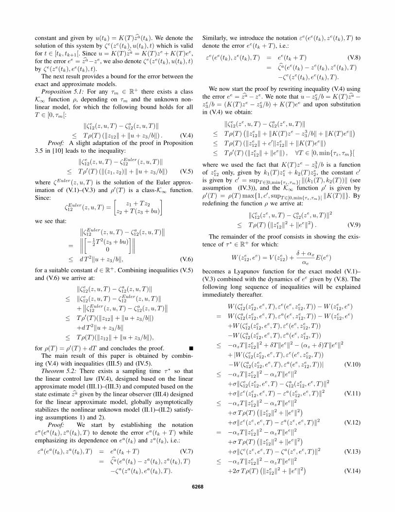
constant and given by u(tk) = K(T )za(tk). We denote the

solution of this system by ζe(ze(tk), u(tk), t) which is valid

for t ∈ [tk, tk+1[. Since u = K(T )za = K(T )ze+K(T )ee,

for the error ee = za−ze, we also denote ζe(ze(tk), u(tk), t)by ζe(ze(tk), e

e(tk), t).The next result provides a bound for the error between the

exact and approximate models.Proposition 5.1: For any τm ∈ R

+ there exists a class

K∞ function ρ, depending on τm and the unknown non-

linear model, for which the following bound holds for all

T ∈ [0, τm[:

‖ζe12(z, u, T )− ζa12(z, u, T )‖≤ Tρ(T ) (‖z12‖+ ‖u+ z3/b‖) . (V.4)

Proof: A slight adaptation of the proof in Proposition

3.5 in [10] leads to the inequality:

‖ζe12(z, u, T )− ζEuler12 (z, u, T )‖

≤ Tρ′(T ) (‖(z1, z2)‖+ ‖u+ z3/b‖) (V.5)

where ζEuler(z, u, T ) is the solution of the Euler approx-

imation of (V.1)–(V.3) and ρ′(T ) is a class-K∞ function.

Since:

ζEuler12 (z, u, T ) =

[z1 + Tz2

z2 + T (z3 + bu)

]we see that: ∥∥ζEuler

12 (z, u, T )− ζa12(z, u, T )∥∥

=

∥∥∥∥[− 1

2T2(z3 + bu)0

]∥∥∥∥≤ d T 2‖u+ z3/b‖, (V.6)

for a suitable constant d ∈ R+. Combining inequalities (V.5)

and (V.6) we arrive at:

‖ζe12(z, u, T )− ζa12(z, u, T )‖≤ ‖ζe12(z, u, T )− ζEuler

12 (z, u, T )‖+∥∥ζEuler

12 (z, u, T )− ζa12(z, u, T )∥∥

≤ Tρ′(T )(‖z12‖+ ‖u+ z3/b‖)+d T 2‖u+ z3/b‖

≤ Tρ(T )(‖z12‖+ ‖u+ z3/b‖),for ρ(T ) = ρ′(T ) + dT and concludes the proof.

The main result of this paper is obtained by combin-

ing (V.4) with inequalities (III.5) and (IV.5).Theorem 5.2: There exists a sampling time τ∗ so that

the linear control law (IV.4), designed based on the linear

approximate model (III.1)–(III.3) and computed based on the

state estimate za given by the linear observer (III.4) designed

for the linear approximate model, globally asymptotically

stabilizes the nonlinear unknown model (II.1)–(II.2) satisfy-

ing assumptions 1) and 2).Proof: We start by establishing the notation

εa(ea(tk), za(tk), T ) to denote the error ea(tk + T ) while

emphasizing its dependence on ea(tk) and za(tk), i.e.:

εa(ea(tk), za(tk), T ) = ea(tk + T ) (V.7)

= ζa(ea(tk)− za(tk), za(tk), T )

−ζa(za(tk), ea(tk), T ).

Similarly, we introduce the notation εe(ee(tk), ze(tk), T ) to

denote the error ee(tk + T ), i.e.:

εe(ee(tk), ze(tk), T ) = ee(tk + T ) (V.8)

= ζa(ee(tk)− ze(tk), ze(tk), T )

−ζe(ze(tk), ee(tk), T ).We now start the proof by rewriting inequality (V.4) using

the error ee = za − ze. We note that u− ze3/b = K(T )za −ze3/b = (K(T )ze − ze3/b) + K(T )ee and upon substitution

in (V.4) we obtain:

‖ζe12(ze, u, T )− ζa12(ze, u, T )‖

≤ Tρ(T )(‖ze12‖+ ‖K(T )ze − z33/b‖+ ‖K(T )ee‖)

≤ Tρ(T ) (‖ze12‖+ c′‖ze12‖+ ‖K(T )ee‖)≤ Tρ′(T ) (‖ze12‖+ ‖ee‖) , ∀T ∈ [0,min{τz, τm}[

where we used the fact that K(T )ze − z33/b is a function

of ze12 only, given by k1(T )ze1 + k2(T )z

e2 , the constant c′

is given by c′ = supT∈[0,min{τz,τm}[ ‖(k1(T ), k2(T ))‖ (see

assumption (IV.3)), and the K∞ function ρ′ is given by

ρ′(T ) = ρ(T )max{1, c′, supT∈[0,min{τz,τm}[ ‖K(T )‖}. By

redefining the function ρ we arrive at:

‖ζe12(ze, u, T )− ζa12(ze, u, T )‖2

≤ Tρ(T )(‖ze12‖2 + ‖ee‖2) . (V.9)

The remainder of the proof consists in showing the exis-

tence of τ∗ ∈ R+ for which:

W (ze12, ee) = V (ze12) +

δ + αx

αeE(ee)

becomes a Lyapunov function for the exact model (V.1)–

(V.3) combined with the dynamics of ee given by (V.8). The

following long sequence of inequalities will be explained

immediately thereafter.

W (ζe12(ze12, e

e, T ), εe(ee, ze12, T ))−W (ze12, ee)

= W (ζa12(ze12, e

e, T ), εa(ee, ze12, T ))−W (ze12, ee)

+W (ζe12(ze12, e

e, T ), εe(ee, ze12, T ))

−W (ζa12(ze12, e

e, T ), εa(ee, ze12, T ))

≤ −αzT‖ze12‖2 + δT‖ee‖2 − (αz + δ)T‖ee‖2+ |W (ζe12(z

e12, e

e, T ), εe(ee, ze12, T ))

−W (ζa12(ze12, e

e, T ), εa(ee, ze12, T ))| (V.10)

≤ −αzT‖ze12‖2 − αzT‖ee‖2+σ‖ζe12(ze12, ee, T )− ζa12(z

e12, e

e, T )‖2+σ‖εe(ze12, ee, T )− εa(ze12, e

e, T )‖2 (V.11)

≤ −αzT‖ze12‖2 − αzT‖ee‖2+σ Tρ(T )

(‖ze12‖2 + ‖ee‖2)+σ‖εe(ze, ee, T )− εa(ze, ee, T )‖2 (V.12)

= −αzT‖ze12‖2 − αzT‖ee‖2+σ Tρ(T )

(‖ze12‖2 + ‖ee‖2)+σ‖ζe(ze, ee, T )− ζa(ze, ee, T )‖2 (V.13)

≤ −αzT‖ze12‖2 − αzT‖ee‖2+2σ Tρ(T )

(‖ze12‖2 + ‖ee‖2) (V.14)

6268

Inequality (V.10) follows from (IV.5) and (III.5). Inequal-

ity (V.11) follows from the function V12 being Lipschitz

continuous with Lipschitz constant σ12

V , function E12 be-

ing Lipschitz continuous with Lipschitz constant σ12

E , and

σ = max{σV , σE}. Inequality (V.13) follows from (V.7)

and (V.8) while inequalities (V.12) and (V.14) result from

a direct application of (V.9).

If we define:

τ∗ = min{τe, τz, τm, ρ−1

( αz

4σd

)}it follows that (V.14) is upper bounded by:

−1

2αzT (‖(ze1, ze2)‖2 + ‖ee‖2)

for all T in the set [tk, tk + τ∗[ thereby showing that W is a

Lyapunov function proving asymptotic stability of (ze1, ze2) =

(0, 0) and ee = (0, 0, 0).Although the discussion so far focused on the asymptotic

stabilization problem, linearity of the model (III.1)–(III.3)

allows us, with the same ease, to design controllers solving

output regulation and tracking problems. The proof of The-

orem 5.2 can easily be adapted so as to also apply to these

cases.

VI. EXPERIMENTAL RESULTS

A. The experimental platform AMBER-3M

AMBER-3M is a planar, modular bipedal robot custom-

built by AMBER Lab (see Fig. 1); here, modular refers to the

fact that it has multiple leg designs that can be attached to test

different walking phenomena [16]. It was previously used for

the study of mechanics-based control [17]. In this particular

study, we used a pair of lower limbs with point feet, which

made AMBER-3M a 5-degree of freedom under-actuated

walking robot. As shown in Fig. 1, the robot is connected

to the world through a planner supporting structure, which

eliminates the lateral motion but does not provide support to

the robot in the sagittal plan.

B. Observer and controller design

In the first set of experiments we immobilized AMBER-

3M while keeping one point foot in the air. The knee

joint corresponding to the free standing point foot was then

controlled by measuring the joint angle via an encoder. The

torque commands produced by the data-driven controller

were transformed, by the ELMO motor driver, into a torque

applied at the knee joint by the BLDC motor. We modeled

the controlled swinging lower limb as an inverted pendulum:

Iθ = u−mg sin θ

where I is the moment of inertia, m is the mass, g is gravity’s

acceleration, θ is the knee angle, and u is the input torque.

Assumption 1) is satisfied since the relative degree of this

system is n = 2. Assumption 2) is also satisfied since the

supposedly unknown function L2fh = −mg sin θ is Lipschitz

continuous, and the function LgL1fh is indeed constant and

given by LgL1fh = b = 1/I = 2.442.

Sampling time τ = 3ms Sampling time τ = 5ms

0 1 2 3-0.1

0

0.1

0.2

0.3

0.4

0 1 2 3-0.1

0

0.1

0.2

0.3

0.4

Sampling time τ = 7ms Sampling time τ = 8ms

0 1 2 3-0.1

0

0.1

0.2

0.3

0.4

0 1 2 3-0.1

0

0.1

0.2

0.3

0.4

Sampling time τ = 9ms Sampling time τ = 10ms

0 1 2 3-0.1

0

0.1

0.2

0.3

0.4

0 1 2 3-0.1

0

0.1

0.2

0.3

0.4

Fig. 2. Angle regulation to the desired set point of 0.35 rad for differentvalues of the sampling time, τ , ranging from 3ms to 10ms.

We designed the linear controller:

u = k1z1 + k2z2 − 1

bz3 (VI.1)

based on the model (III.1)–(III.3). The gains k1 and k2 were

chosen so as to place the closed-loop eigenvalues at e−λτ

with λ = 20. This resulted in:

k1 = −e−2λτ (eλτ − 1)2

bτ2, k2 =

−3 + 2e−λτ + e−2λτ

2bτ.

This controller was then used with the estimate za of

za computed by a Luenberger observer whose gain was

designed to place its eigenvalues at e−mλτ with m = 3.

This lead to the gain matrix:

L =[l1 l2 l3

]T, l1 = 3− 3e−mλτ

l2 = e−3mλτ (emλτ−1)2(5emλτ+1)2τ , l3 = e−3mλτ (emλτ−1)3

τ2 .

C. Set-point regulation

Theorem 5.2 asserts the existence of a sufficiently small

sampling time for which the previously described controller

and observer stabilize the free standing point foot. In this

experiment we decreased the sampling time, starting from

10ms, until adequate performance for set-point regulation

of the angle to the value of 0.35 rad was observed. Fig. 2

shows that adequate performance is achieved with sampling

times smaller than or equal to 8ms. Based on these results,

we used a sampling time of 5ms in all the other experiments.

To illustrate how the proposed control technique is robust

to the value of b, assumed to be known, we repeated the

6269

0 1 2 3-0.1

0

0.1

0.2

0.3

0.4

0 1 2 3-0.1

0

0.1

0.2

0.3

0.4

Fig. 3. Angle regulation to the desired set point of 0.35 rad when usingan incorrect value for b. Left figures: b = 1.8, right figures: b = 4.

35 40 45 50

0.65

0.7

0.75

0.8

0.85

35 40 45 50

0.65

0.7

0.75

0.8

0.85

Fig. 4. Tracking performance on left (PD control) and right (data-drivencontrol) for the knee joint while walking.

experiment with τ = 5ms and ranging b from 1.8 to 4 (the

true value of b is 2.442). The top part of Figure 3 shows

the evolution of the knee angle for b = 1.8 and b = 4.

We observe that the regulation objective is still met although

there is a larger overshoot and slower convergence for b = 4.

D. Comparison between the data driven controller and a PDcontroller

In this last experiment we compared the trajectory tracking

capabilities of the data driven controller with a Proportional-

Derivative (PD) controller that had been used in the past to

implement walking gaits on AMBER-3M. This comparison

was performed while the robot walked. Note that the pendu-

lum model for the knee joint is no longer valid in the context

of a walking gait where there are two distinct phases: the

swinging phase where the lower limb does not make contact

with the ground and the standing phase during which the

weight of the whole robot is supported by the lower limb.

Additionally, there are impacts due to foot strike (the robot is

governed by a hybrid system model in this case). As shown

in the movie [18], despite these considerations, we find that

the data-driven controller performs well.

The tracking error associated with the PD controller can be

seen in Fig. 4 by observing the difference between the actual

and desired behavior. This figure also shows the tracking

performance of the data-driven controller while the robot is

locomoting, wherein it clearly outperforms the PD controller.

VII. CONCLUSIONS

The results described in this paper are but a first step

towards a general purpose data driven control methodology.

The authors are currently working on several extensions such

as: 1) relaxing feedback linearizability to partial feedback lin-

earizability (this will require making certain assumptions on

the residual and zero-dynamics); 2) identifying the function

LgLn−1f h from data (this is a classical and hard adaptive

control problem that becomes simpler when the sign of

LgLn−1f h is known since we can use, e.g., Lyapunov based

controller based adaptive controllers based on the Immersion

and Invariance approach [19]). Also under investigation are

the robustness properties of the proposed control method-

ology, especially in what regards sensor noise. Although it

is unavoidable that model-free controllers are more sensitive

to noise than model-based controllers, since all the model

information needs to be extracted from data, it is important

to quantify such sensitivity.

REFERENCES

[1] M. Fliess, C. Join, and H. Sira-Ramırez, “Complex continuous non-linear systems: Their black box identification and their control,” IFACProceedings Volumes, vol. 39, no. 1, pp. 416 – 421, 2006.

[2] M. Fliess and C. Join, “Commande sans modele et commande amodele restreint,” in e-STA Sciences et Technologies de l’Automatique,SEE - Societe de l’Electricite, de l’Electronique et des Technologiesde l’Information et de la Communication, vol. 5, 2008, pp. 1–23.

[3] M. Fliess and C. Join, “Model-free control and intelligent PID con-trollers: Towards a possible trivialization of nonlinear control?” IFACProceedings Volumes, vol. 42, no. 10, pp. 1531 – 1550, 2009.

[4] C. Sierra, E. Tseng, A. Jain, and H. Peng, “Cornering stiffness esti-mation based on vehicle lateral dynamics,” Vehicle System Dynamics,vol. 44, pp. 24–38, 2006.

[5] M. W. Spong, S. Hutchinson, and M. Vidyasagar, Robot modeling andcontrol. wiley New York, 2006, vol. 3.

[6] R. M. Murray, Z. Li, S. S. Sastry, and S. S. Sastry, A mathematicalintroduction to robotic manipulation. CRC press, 1994.

[7] M. Fliess and C. Join, “Model-free control,” International Journal ofControl, vol. 86, no. 12, pp. 2228–2252, 2013.

[8] M. Arcak and D. Nesic, “A framework for nonlinear sampled-dataobserver design via approximate discrete-time models and emulation,”Automatica, vol. 40, pp. 1931–1938, 2004.

[9] D. Nesic and A. Teel, “A framework for stabilization of nonlinearsampled-data systems based on their approximate discrete-time mod-els,” IEEE Transactions on Automatic Control, vol. 49, pp. 1103–1034,2004.

[10] D. Laila, D.Nesic, and A.Astolfi, “Sampled-data control of nonlinearsystems,” in Advanced topics in control systems theory II, ser. LectureNotes in Control and Information Science, A. Loria, F. Lamnabhi-Lagarrigue, and E. Panteley, Eds. Springer-Verlag, 2006, vol. 328,pp. 91–137.

[11] M. Fliess and H. Sira-Ramırez, “An algebraic framework for linearidentification,” ESAIM: Control, Optimisation and Calculus of Varia-tions, vol. 9, pp. 151 – 168, 2003.

[12] M. Fliess and H. Sira-Ramırez, Closed-loop Parametric Identificationfor Continuous-time Linear Systems via New Algebraic Techniques.London: Springer London, 2008, pp. 363–391.

[13] F. Mazenc, L. Praly, and W. Dayawansa, “Global stabilization byoutput feedback: examples and counterexamples,” Systems & ControlLetters, vol. 23, no. 2, pp. 119 – 125, 1994.

[14] J. Reger and J. Jouffroy, “On algebraic time-derivative estimationand deadbeat state reconstruction,” in Proceedings of the 48h IEEEConference on Decision and Control (CDC) held jointly with 200928th Chinese Control Conference, 2009, pp. 1740–1745.

[15] P. J. Antsaklis and A. N. Michel, Linear Systems. McGraw-Hill,1997.

[16] E.R.Ambrose, W.L.Ma, C.M.Hubicki, and A.D.Ames, “Toward bench-marking locomotion economy across design configurations on themodular robot: AMBER-3M,” in 1st IEEE Conference on ControlTechnology and Applications, 2017.

[17] M. J. Powell, W. L. Ma, E. R. Ambrose, and A. D. Ames, “Mechanics-based design of underactuated robotic walking gaits: Initial experimen-tal realization,” in 2016 IEEE-RAS 16th International Conference onHumanoid Robots (Humanoids), Nov 2016, pp. 981–986.

[18] AMBER-3M walking with data-driven controller:https://youtu.be/wzL9O3FOHyA.

[19] A. Astolfi, D. Karagiannis, and R. Ortega, Nonlinear and AdaptiveControl with Applications, ser. Communications and Control Engi-neering. Springer-Verlag, 2008.

6270