International Conference onInformation, Communications,

and Signal ProcessingSingapore

9 September 1997

Fundamentals ofData Compression

Robert M. GrayInformation Systems Laboratory

Department of Electrical EngineeringStanford University

rmgray@stanford.edu

http://www-isl.stanford.edu/~gray/

c©Robert M. Gray, 1997

Part I Introduction and Overview

Part II Lossless Compression

Part III Lossy Compression

Part IV “Optimal” Compression

Closing Observations

2

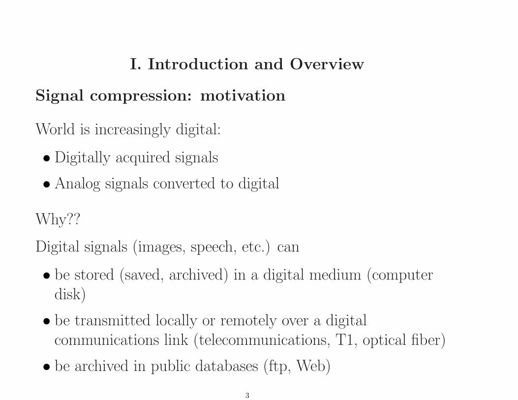
I. Introduction and Overview

Signal compression: motivation

World is increasingly digital:

• Digitally acquired signals

• Analog signals converted to digital

Why??

Digital signals (images, speech, etc.) can

• be stored (saved, archived) in a digital medium (computerdisk)

• be transmitted locally or remotely over a digitalcommunications link (telecommunications, T1, optical fiber)

• be archived in public databases (ftp, Web)

3

• be processed by computer:

– computer assisted diagnosis/decision

– automatic search for specified patterns

– context searches

– highlight or mark interesting suspicious regions

– focus on specific regions of image intensity

– statistical signal processing

∗ enhancement/restoration

∗ denoising

∗ classification/detection

∗ regression/estimation/prediction

∗ feature extraction/pattern recognition

∗ filtering

4

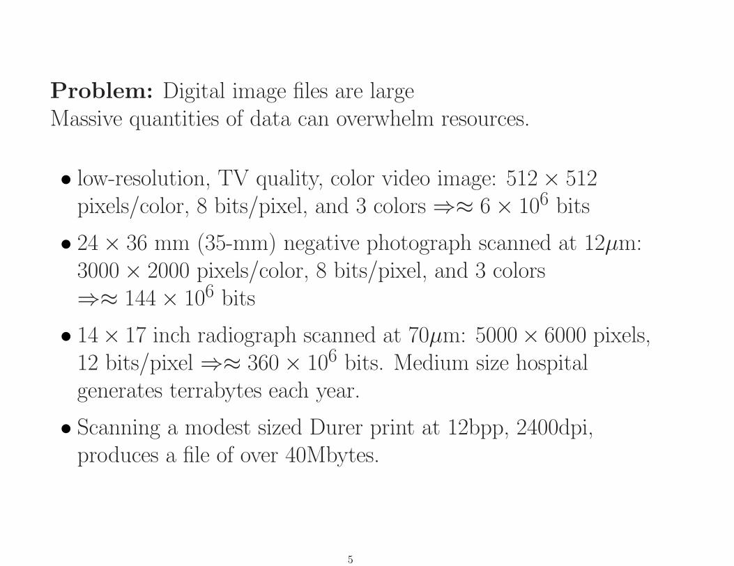
Problem: Digital image files are largeMassive quantities of data can overwhelm resources.

• low-resolution, TV quality, color video image: 512× 512pixels/color, 8 bits/pixel, and 3 colors⇒≈ 6× 106 bits

• 24× 36 mm (35-mm) negative photograph scanned at 12µm:3000× 2000 pixels/color, 8 bits/pixel, and 3 colors⇒≈ 144× 106 bits

• 14× 17 inch radiograph scanned at 70µm: 5000× 6000 pixels,12 bits/pixel⇒≈ 360× 106 bits. Medium size hospitalgenerates terrabytes each year.

• Scanning a modest sized Durer print at 12bpp, 2400dpi,produces a file of over 40Mbytes.

5

• LANDSAT Thematic Mapper scene: 6000× 6000pixels/spectral band, 8 bits/pixel, and 6 nonthernmal spectralbands ⇒≈ 1.7× 109 bits

Solution?

6

Compression required for ef-ficient transmission

• send more data in avail-able bandwidth

• send the same data in lessbandwidth

• more users on same samebandwidth

and storage

• can store more data

• can compress for localstorage, put details oncheaper media

7

Also useful for progressive reconstruction, scalable delivery,browsing

and as a front end to other signal processing.

Future: Combine compression and subsequent user-specificprocessing.

8

General types of compression

Lossless compression

noiseless coding, lossless coding, invertible coding, entropycoding, data compaction.

• Can perfectly recover original data (if no storage ortransmission bit errors).

• Variable length binary codewords (or no compression)

• Only works for digital sources.

General idea: Code highly probable symbols into short binarysequences, low probability symbols into long binary sequences, sothat average is minimized.

9

Morse code Consider dots and dashes as binary.

Chose codeword length inversely proportional to letter relativefrequencies

Huffman code 1952, in unix compact utility and manystandards

run-length codes popularized by Golomb in early 1960s, usedin JPEG standard

Lempel-Ziv(-Welch) codes 1977,78 in unix compressutility, diskdouble, stuffit, stacker, PKzip, DOS, GIF

lots of patent suits

arithmetic codes Fano, Elias, Rissanen, Pasco

IBM Q-coder

10

Warning: To get average rate down, need to let maximuminstantaneous rate grow. This means that can get dataexpansion instead of compression in the short run.

Typical lossless compression ratios: 2:1 to 4:1Can do better on specific data types

11

Lossy compression

Not invertible, information lost.

Disadvantage: Lose information and quality, but if have enough(?) bits, loss is invisible.

Advantage: Greater compression possible. (6:1 to 16:1 typical,80:1 to 100:1 promising in some applications)

Design Goal: Get “best” possible quality for available bits.

Big issue: is “best” good enough?

Examples: DPCM, ADPCM, transform coding, LPC, H.26*,JPEG, MPEG, EZW, SPHIT, CREW, StackRun

12

In between: “perceptually lossless”(Perhaps) need not retain accuracy past

• what the eye can see (which may depend on context),

• the noise level of the acquisition device,

• what can be squeezed through a transmission or storagechannel, i.e., an imperfect picture may be better than nopicture at all.

This can be controversial (fear of lurking lawyers if misdiagnoseusing “lossy” reproduction, even if “perceptually lossless”)

Is lossy compression acceptable?

NO in some applications: Computer programs, bankstatements, espionage

Thought necessary for Science and Medical Images.

Is it??13

Loss may be unavoidable, may have to choose between imperfectimage or no data at all (or long delays).

Loss not a problem with

• Followup studies

• Archives

• Research and Education

• Progressive reconstruction.

• Entertainment

Growing evidence suggests lossy compression does not damagediagnosis.

In general lossy compression may also include a losslesscompression component, to squeeze a few more bits out.

14

Compression Context

• Compression is usually part of general system for dataacquisition, transmission, storage, and display.

• Analog-to-digital conversion and digital acquisition.

• Quality and utility of “modified” digital images.

15

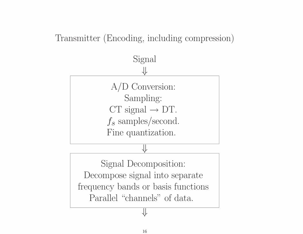
Transmitter (Encoding, including compression)

Signal⇓

A/D Conversion:Sampling:

CT signal → DT.fs samples/second.Fine quantization.

⇓Signal Decomposition:

Decompose signal into separatefrequency bands or basis functions

Parallel “channels” of data.

⇓

16

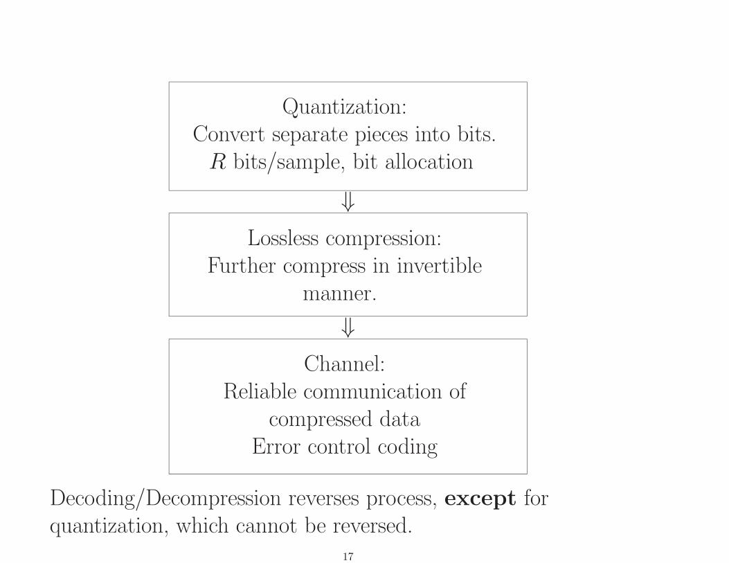
Quantization:Convert separate pieces into bits.R bits/sample, bit allocation

⇓Lossless compression:

Further compress in invertiblemanner.

⇓Channel:

Reliable communication ofcompressed data

Error control coding

Decoding/Decompression reverses process, except forquantization, which cannot be reversed.

17

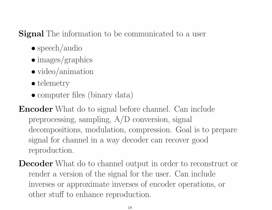
Signal The information to be communicated to a user

• speech/audio

• images/graphics

• video/animation

• telemetry

• computer files (binary data)

Encoder What do to signal before channel. Can includepreprocessing, sampling, A/D conversion, signaldecompositions, modulation, compression. Goal is to preparesignal for channel in a way decoder can recover goodreproduction.

Decoder What do to channel output in order to reconstruct orrender a version of the signal for the user. Can includeinverses or approximate inverses of encoder operations, orother stuff to enhance reproduction.

18

Channel Portion of communication system out of designer’scontrol: random or deterministic alteration of signal. E.g.,addition of random noise, linear or nonlinear filtering.

*transparent channel *wireless (aka radio)deep space *satellitetelephone lines (POTS, ISDN, fiber) *ethernetfiber *CDmagnetic tape *magnetic diskcomputer memory *modem

Often modeled as linear filtering + conditional probabilitydistribution

Here ignore the channel coding/error control portion, save foranecdotal remarks.

Consider individual components

Sometimes combined. Sometimes omitted.19

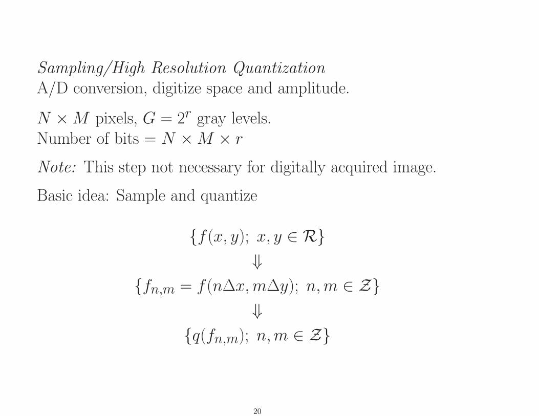
Sampling/High Resolution QuantizationA/D conversion, digitize space and amplitude.

N ×M pixels, G = 2r gray levels.Number of bits = N ×M × rNote: This step not necessary for digitally acquired image.

Basic idea: Sample and quantize

{f(x, y); x, y ∈ R}⇓

{fn,m = f(n∆x,m∆y); n,m ∈ Z}⇓

{q(fn,m); n,m ∈ Z}

20

The Brig Grand Turk

Most compression work assumes a digital input as a startingpoint since DSP is used to accomplish the compression.

21

-5 0 5 10 15 20 25 30 35 40 45

0

5

10

15

20

25

30

35

22

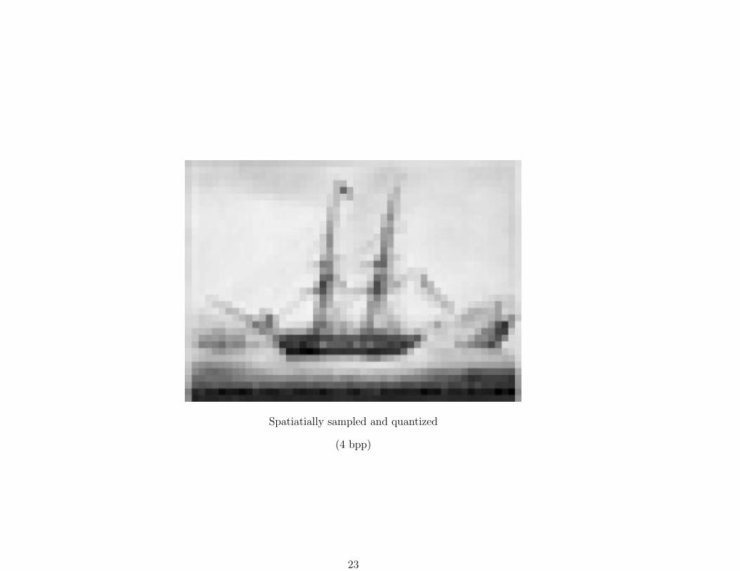
Spatiatially sampled and quantized

(4 bpp)

23

Signal decomposition (transformation, mapping): Decomposeimage into collection of separate images (bands, coefficients)

E.g., Fourier, DCT, wavelet, subband.

Also: Karhunen-Loeve, Hotelling, Principal ValueDecomposition, Hadamard, Walsh, Sine, Hartley, Fractal

(Typically done digitally.)

Why transform?

24

Several reasons:

• Good transforms tend to compact energy into a fewcoefficients, allowing many to be quantized to 0 bits withoutaffecting quality.

• Good transforms tend to decorrelate (reduce lineardependence) among coefficients, causing scalar quantizers tobe more efficient. (folk theorem)

• Good transforms are effectively expanding the signals in goodbasis functions. (Mathematical intuition.)

• The eye and ear tend be sensitive to behavior in the frequencydomain, so coding in the frequency domain allows the use ofperceptually based distortion measures, e.g., incorporatingmasking.

25

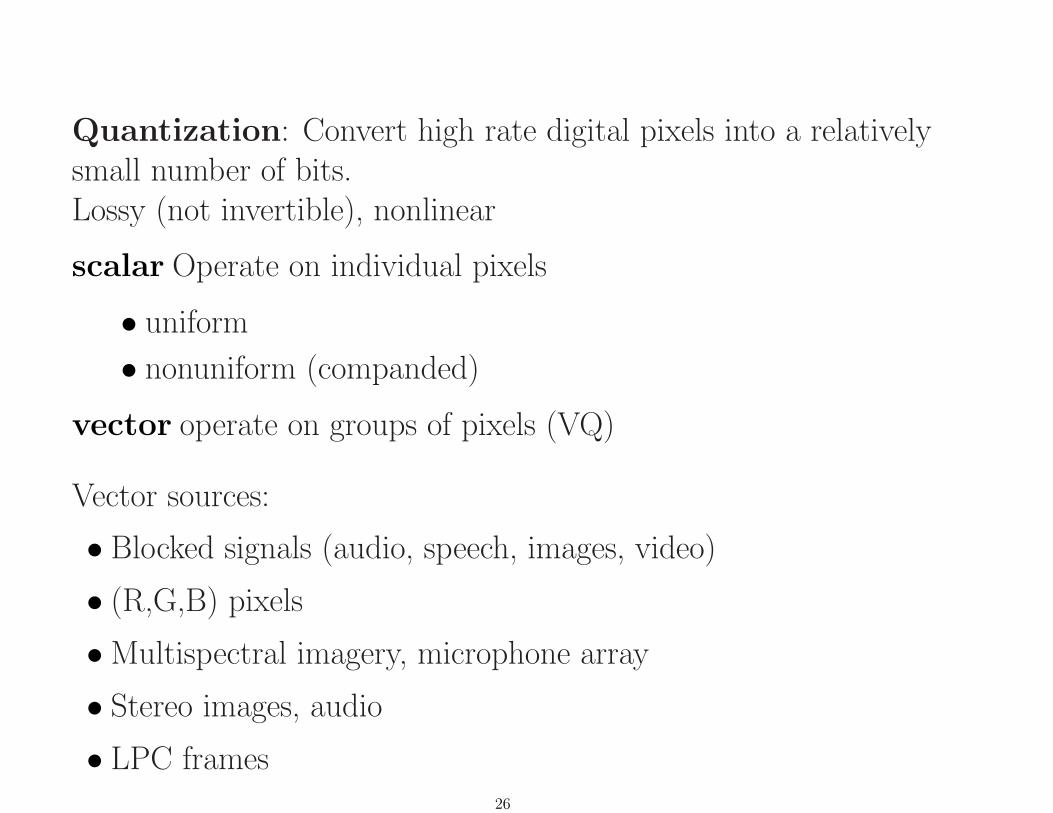
Quantization: Convert high rate digital pixels into a relativelysmall number of bits.Lossy (not invertible), nonlinear

scalar Operate on individual pixels

• uniform

• nonuniform (companded)

vector operate on groups of pixels (VQ)

Vector sources:

• Blocked signals (audio, speech, images, video)

• (R,G,B) pixels

•Multispectral imagery, microphone array

• Stereo images, audio

• LPC frames26

Codeword assignment (“Coding” (Lossless compression,Entropy Coding): binary words are chosen to represent whatcomes out of the quantization step.

Desirable attributes of compression/coding:

• Successive approximation/progressive reconstructionEach additional bit improves accuracy of signal, don’t need towait for all bits to start.

• Scalable: Same bit stream produces different quality/costoptions (rate, complexity, power, . . . )

Decoding/Decompression reverses process, except forquantization, which cannot be reversed.

27

Quantization involved in

• A/D conversion (high resolution quantization)

• digital arithmetic, errors in transforms

• quantization for lossy compression

For computer applications can view original signal as alreadydigital, yielding a general compression encoder block diagram:

OriginalSignal

-Signal

Decomposition - Quantization -LosslessCoding -

CompressedBit Stream

Typical Compression System

28

Important parameters of compression systems

• Compression efficiency • Bitrate and compression ratio.

• Fidelity, average distortion • MSE, SNR, subjective

• Complexity • algorithmic, hardware, cost

•Memory

• Coding Delay

• Robustness

29

Issues in Research and Practice

• encoder and decoder structures

• encoder and decoder algorithms

• encoder and decoder design and optimization

• encoder and decoder performance (R,D)

• encoder and decoder complexity/cost

• theoretical bounds and limits

• Overall quality in application: Subjective quality anddiagnostic accuracy

• systems and standards

30

Other issues:

• Variable-rate vs. fixed-rate

• Bitrate control

• Progressive, scalable (power, bitrate, cost, complexity)

31

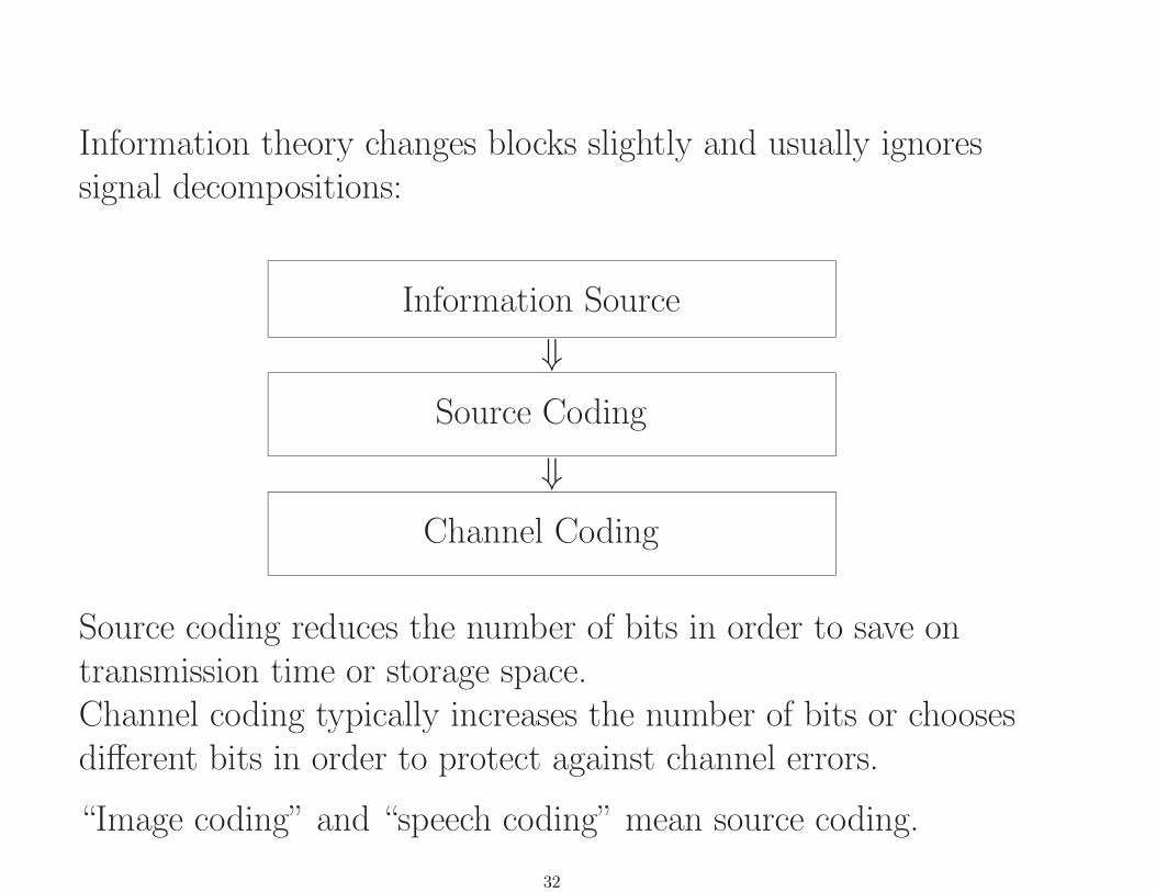
Information theory changes blocks slightly and usually ignoressignal decompositions:

Information Source

⇓Source Coding

⇓Channel Coding

Source coding reduces the number of bits in order to save ontransmission time or storage space.Channel coding typically increases the number of bits or choosesdifferent bits in order to protect against channel errors.

“Image coding” and “speech coding” mean source coding.

32

“Error correction coding” means channel coding.

Information theory (Shannon)⇒ for single source, single user,can do nearly optimally if separately source and channel code.NOT true in networks! Better to consider jointly.

Care needed, channel errors can have catastrophic effects onreconstructing compressed data.Some work done on joint source-channel coding. Someconsideration given to the effect of bit errors.Catastrophic errors vs. minor errors of fixed rate schemes.

33

If enough bits (samples and quantizer values), cannot tell thedifference between original and digital version.

But how much is enough and how do you prove it?

How much can you compress?Do you lose important information?Do you get sued?

Survey the field of compression: methods, theory, and standards.

Some critiques and personal biases.

For a list of many compression-related Web sites withdemonstrations, examples, explanations, and software, visit

http://www-isl.stanford.edu/~gray/iii.html

34

Part II. Lossless Coding

noiseless coding, entropy coding, invertible coding, datacompaction.In much of CS world simply called “data compression”

• Can perfectly recover original data (if no storage ortransmission bit errors) transparent

• Variable length binary codewords.

• Only works for digital sources.

• Can also expand data!

35

Simple binary invertible code:Example: fixed length (rate) code

Input Letter Codeworda0 00a1 01a2 10a3 11

Can uniquely decode individual codewords and sequences if knowwhere blocks start. E.g.,0000011011 decodes as a0a0a1a2a3.

Real world example:ASCII (American Standard Code for Information Interchange):assigns binary numbers to all letters, numbers, punctuation foruse in computers and digital communication and storage.

All letters have same number of binary symbols (7).36

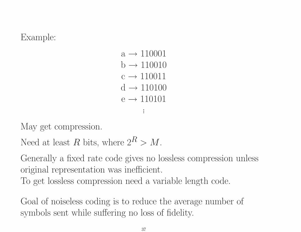
Example:

a → 110001b → 110010c → 110011d → 110100e → 110101

...

May get compression.

Need at least R bits, where 2R > M .

Generally a fixed rate code gives no lossless compression unlessoriginal representation was inefficient.To get lossless compression need a variable length code.

Goal of noiseless coding is to reduce the average number ofsymbols sent while suffering no loss of fidelity.

37

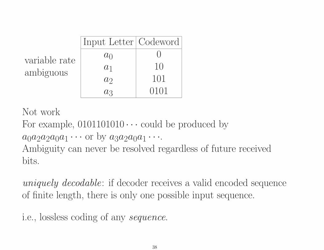
variable rateambiguous

Input Letter Codeworda0 0a1 10a2 101a3 0101

Not workFor example, 0101101010 · · · could be produced bya0a2a2a0a1 · · · or by a3a2a0a1 · · ·.Ambiguity can never be resolved regardless of future receivedbits.

uniquely decodable: if decoder receives a valid encoded sequenceof finite length, there is only one possible input sequence.

i.e., lossless coding of any sequence.

38

variable rateuniquely decodable

Input Letter Codeworda0 0a1 10a2 110a3 111

Goal of noiseless coding is to reduce the average number ofsymbols sent while suffering no loss of fidelity. Basic approaches:

• Statistical: Code likely symbols or sequences with short binarywords, unlikely with long. (Morse code, runlength coding,Huffman coding, Fano/Elias codes, arithmetic codes)

• Dictionary: Build a table of variable length sequences as theyoccur and then index into table. (Lempel-Ziv codes)

39

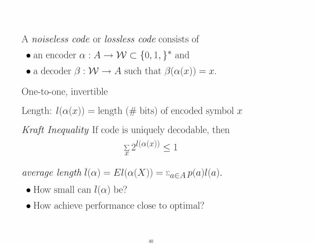
A noiseless code or lossless code consists of

• an encoder α : A→W ⊂ {0, 1, }∗ and

• a decoder β :W → A such that β(α(x)) = x.

One-to-one, invertible

Length: l(α(x)) = length (# bits) of encoded symbol x

Kraft Inequality If code is uniquely decodable, then∑x

2l(α(x)) ≤ 1

average length l(α) = El(α(X)) = ∑a∈A p(a)l(a).

• How small can l(α) be?

• How achieve performance close to optimal?

40

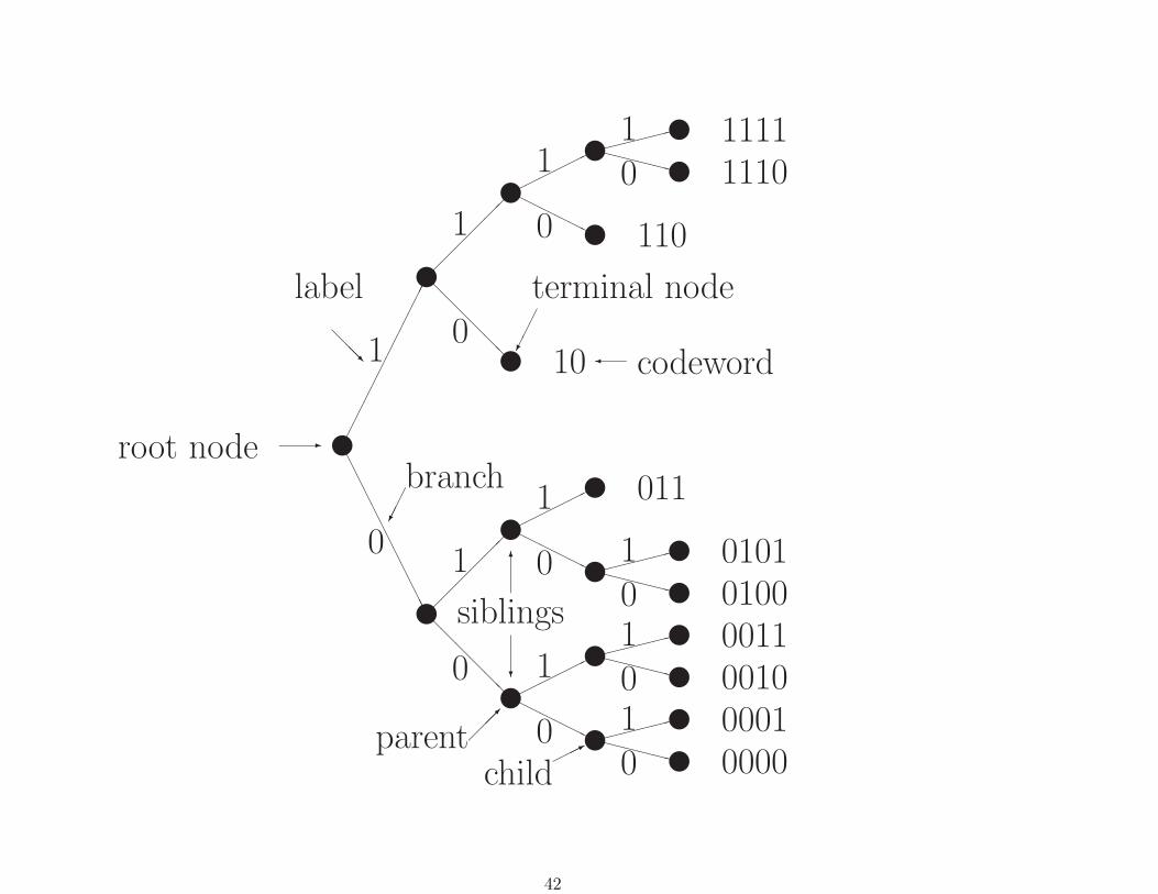
Prefix and Tree-structured Codes

Prefix condition: No codeword is a prefix of another codeword.

Ensures uniquely decodable.

Essentially no loss of generality.Binary prefix codes can be depicted as a binary tree:

41

}-root node ������������

1

label

@@@R

}������

1}�����

�1}������1 } 1111XXXXXX0 } 1110

HHHHHH0 } 110@@@@@@

0 } 10 � codeword

terminal node����

AAAAAAAAAAAA

0

branch����

}������

1}�����

�1} 011

HHHHHH0 }������1 } 0101XXXXXX0 } 0100

@@@@@@

0 }����

parent

����

��1}������1 } 0011XXXXXX0 } 0010

HHHHHH0 }���*

child���

���1 } 0001XXXXXX0 } 0000

siblings

6

?

42

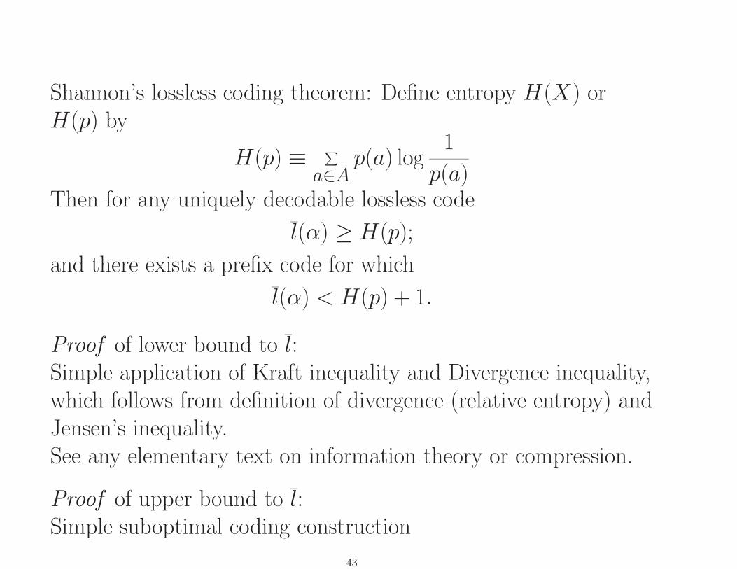
Shannon’s lossless coding theorem: Define entropy H(X) orH(p) by

H(p) ≡ ∑a∈A

p(a) log1

p(a)Then for any uniquely decodable lossless code

l(α) ≥ H(p);

and there exists a prefix code for which

l(α) < H(p) + 1.

Proof of lower bound to l:Simple application of Kraft inequality and Divergence inequality,which follows from definition of divergence (relative entropy) andJensen’s inequality.See any elementary text on information theory or compression.

Proof of upper bound to l:Simple suboptimal coding construction

43

Huffman: simple algorithm yielding the optimum code in thesense of providing the minimum average length over all uniquelydecodable codes.

Notes

• “optimum” for specified code structure, i.e., memorylessoperation on each successive symbol

• assumes that underlying pmf p is known

44

Huffman Codes:Based on following facts (proved in any compression orinformation theory text)A prefix code is optimal if it has the following properties:

• If symbol a is more probable than symbol b (p(a) > p(b))then l(a) ≤ l(b)

• The two least probable input symbols have codewords whichare equal in length and differ only in the final symbol

Huffman gave a constructive algorithm for designing such a code.The input alphabet symbols can be considered to correspond tothe terminal nodes of a code tree . “Grow” trea from leaves toroot, each time satisfying optimality conditions

45

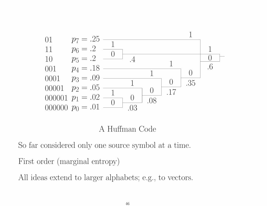
000000000001000010001001101101

p0 = .01p1 = .02p2 = .05p3 = .09p4 = .18p5 = .2p6 = .2p7 = .25

01

0

1

.03

0

1

.08

0

1

.17

0

1

.35

01

.6

01

.4

A Huffman Code

So far considered only one source symbol at a time.

First order (marginal entropy)

All ideas extend to larger alphabets; e.g., to vectors.

46

Code XN = (X0, · · · , XN−1) ∼ pXN

Shannon:For any integer N average length satisfies

l ≥ 1

NH(XN ).

There exists a prefix code for which

l <1

NH(XN ) +

1

N.

For any fixed N , Huffman optimal.

If process stationary, entropy rate

H = minN

H(XN )

N= limN→∞

H(XN )

N.

is impossible to beat, and asymptotically achievable by codingvery large blocks.

47

Question If “optimal” and can get arbitrarily close totheoretical limit, why not always use?

Because too complicated : Big N needed, which can makeHuffman tables enormous.

Also: Do not always know distributions, and they can change.

48

Leads to many methods that are “suboptimal,” but whichoutperform any (implementable) Huffman code.

Good ones are also asymptotically optimal, e.g., arithmetic andLempel-Ziv.

Note: codes have global block structure on a sequence, butlocally they operate very differently. Nonblock, memory

Note: Frequently someone announces a lossless code that doesbetter than the Shannon optimum.

Usually a confusion of first order entropy with entropy rate, oftena confusion of what “optimal” means or what the constraints are.

49

Arithmetic codes

Finite-precision version of Elias (& Fano)code developed byPasco and Rissanen.Heart of IBM Q-coder.

Here consider only special case of lossless coding a binary iidsource {Xn} with Pr(Xn = 1) = p and Pr(Xn = 0) = q.(It is convenient to give a separate name to q = 1− p.)

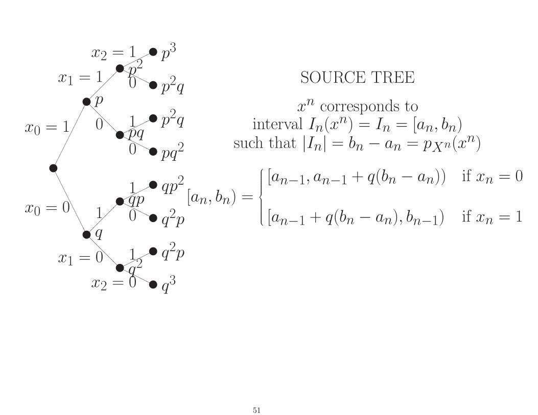
Key idea: Produce a code that results in codelengths near theShannon optimal, i.e., code a sequence xn = (x0, x1, . . . , xn−1)into a codeword uL where L = l(xn) ≈ − log pXn(xn).

50

{����������

x0 = 1

{p�����x1 = 1{p2

@@@@@

0 {pq

AAAAAAAAAA

x0 = 0

{q�����

1{qp

@@@@@

x1 = 0 {q2

�����x2 = 1 {p3

HHHHH0 {p2q

�����1 {p2q

HHHHH0 {pq2

�����1 {qp2

HHHHH0 {q2p

�����1 {q2p

HHHHHx2 = 0 {q3

SOURCE TREE

xn corresponds tointerval In(xn) = In = [an, bn)

such that |In| = bn − an = pXn(xn)

[an, bn) =

[an−1, an−1 + q(bn − an)) if xn = 0

[an−1 + q(bn − an), bn−1) if xn = 1

51

{����������

x0 = 1

{p�����x1 = 1{p2

@@@@@

0 {pq

AAAAAAAAAA

x0 = 0

{q�����

1{qp

@@@@@

x1 = 0 {q2

�����x2 = 1 {p3

HHHHH0 {p2q

�����1 {p2q

HHHHH0 {pq2

�����1 {qp2

HHHHH0 {q2p

�����1 {q2p

HHHHHx2 = 0 {q3 0.0

1.0

p

q

p2

pq

qp

q2

p3

···

q3

52

{����������

1

{�����

1{

@@@@@

0 {

AAAAAAAAAA{���

��

1{

@@@@@

0 {

�����1 {

HHHHH0 {

�����1 {

HHHHH0 {

�����1 {

HHHHH0 {

�����1 {

HHHHH0 {

CODE TREE

uL corresponds tointerval JL such that |JL| = 2−L

JL = [∑L−1l=0 ul2

−l−1, ∑L−1l=0 ul2

−l−1 + 2−L)

53

{����������

1

{�����

1{

@@@@@

0 {

AAAAAAAAAA{���

��

1{

@@@@@

0 {

�����1 {

HHHHH0 {

�����1 {

HHHHH0 {

�����1 {

HHHHH0 {

�����1 {

HHHHH0 { 0.0

1.0

12

12

14

14

14

14

18

···

18

54

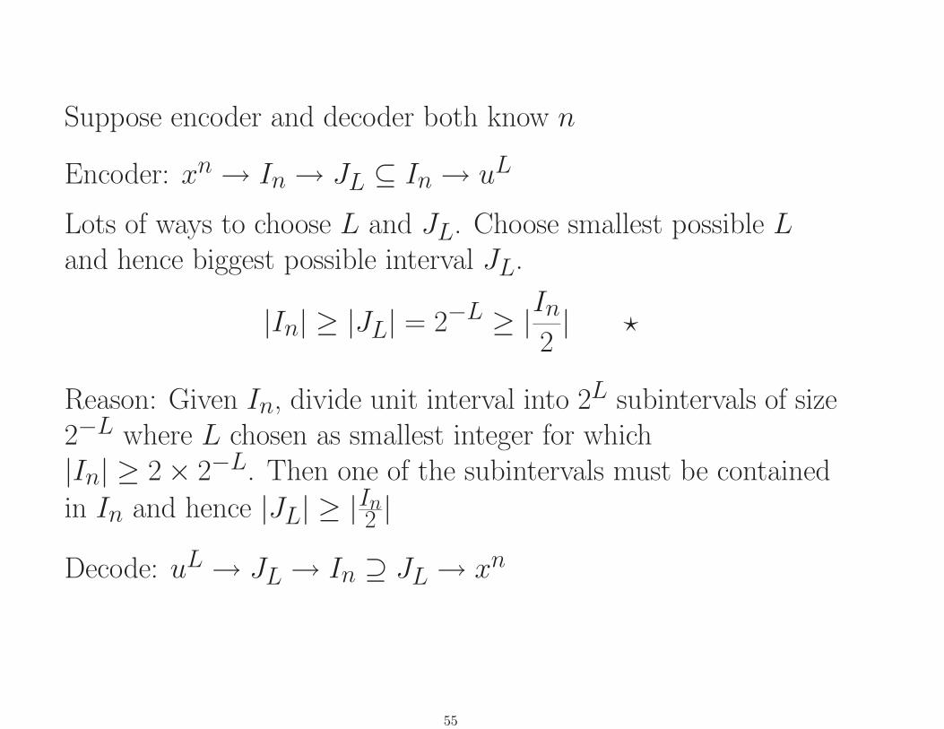
Suppose encoder and decoder both know n

Encoder: xn→ In→ JL ⊆ In→ uL

Lots of ways to choose L and JL. Choose smallest possible Land hence biggest possible interval JL.

|In| ≥ |JL| = 2−L ≥ |In2| ?

Reason: Given In, divide unit interval into 2L subintervals of size2−L where L chosen as smallest integer for which|In| ≥ 2× 2−L. Then one of the subintervals must be contained

in In and hence |JL| ≥ |In2 |

Decode: uL→ JL→ In ⊇ JL→ xn

55

Key fact: Taking logarithms implies that

− log |In| ≤ L ≤ − log |In2|

− log pXn(xn) ≤ L ≤ − logpXn(xn)

2= − log pXn(xn) + 1

Thus if xn→ JL, then

− log pXn(xn) ≤ l(α(xn)) =≤ − log pXn(xn) + 1

or

so l(xn) ≈ − log pXn(xn) as desired.

56

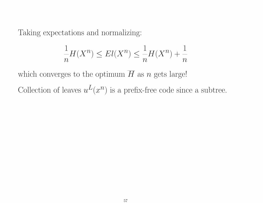
Taking expectations and normalizing:

1

nH(Xn) ≤ El(Xn) ≤ 1

nH(Xn) +

1

n

which converges to the optimum H as n gets large!

Collection of leaves uL(xn) is a prefix-free code since a subtree.

57

Why “better” than Huffman?

Incrementality of algorithm permits much larger n then doesHuffman. E.g., suppose n = 256× 256 for a modest size image.

Huffman out of the question, would need a tree of depth 265536.

Elias encoder can compute [ak, bk) incrementally ask = 1, 2, . . . , n.

As Ik shrinks, can send “release” bits incrementally: Send up tol bits where

Jl ⊇ Ik,

Jl is the smallest interval containing Ik.Decoder receives Jl, can decode up to xm, where

Im ⊇ Jl ⊇ Ik, where m < k.

58

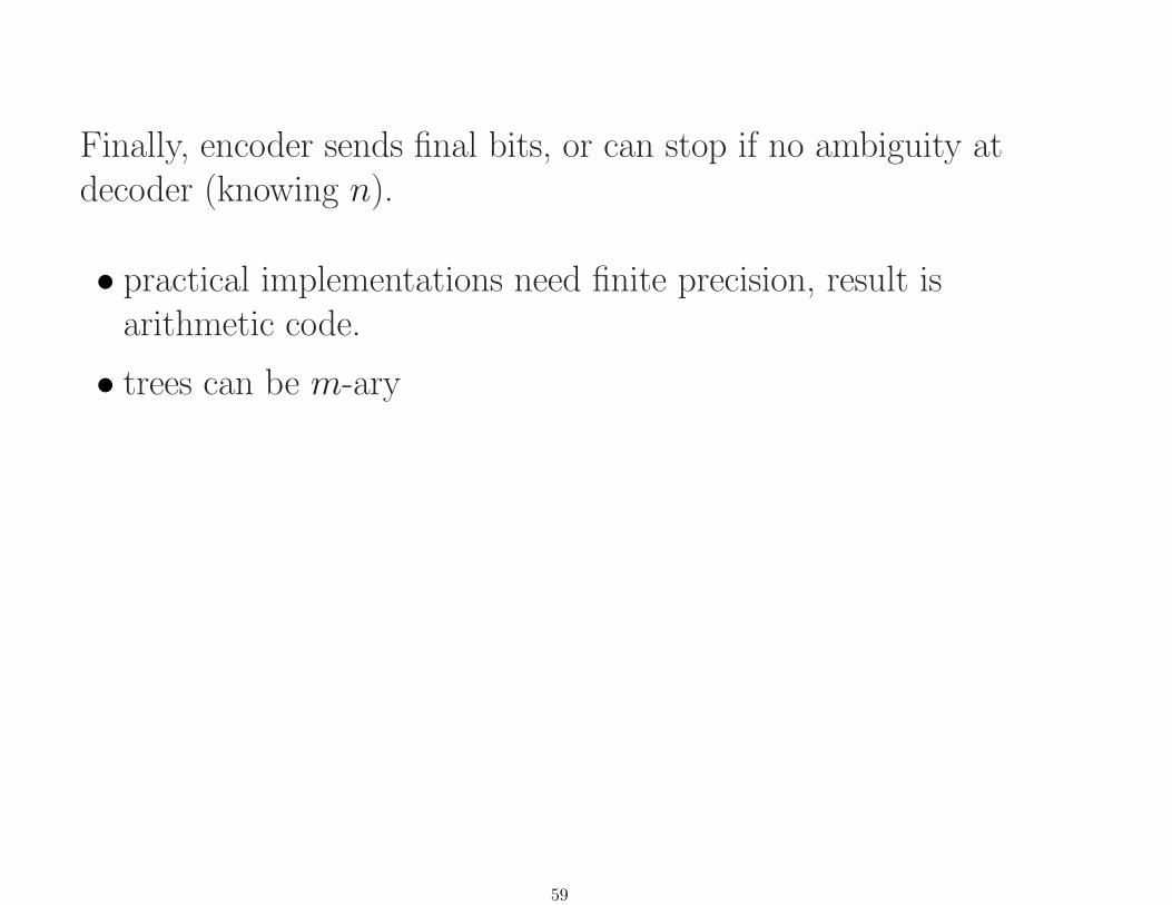
Finally, encoder sends final bits, or can stop if no ambiguity atdecoder (knowing n).

• practical implementations need finite precision, result isarithmetic code.

• trees can be m-ary

59

Extend to sources with memory by using “context modeling”Compute

[an.bn) =

[an−1, an−1 + (bn−1 − an−1) Pr(Xn = 0|xn−1)) if xn = 0[an−1 + (bn−1 − an−1) Pr(Xn = 0|xn−1), bn−1) if xn = 1

Pr(Xn = 0|xn−1)) can be learned on the fly, e.g., assumeMarkov order and estimate from histograms.

Adaptive arithmetic codes: learn conditional pmf’s on the fly.

Performance depends on how well (accuracy and complexity)estimate underlying conditional distributions.

Witten, Bell, & Cleary

60

Adaptive and Universal Entropy Coding:

Both Huffman codes and arithmetic codes assume a prioriknowledge of the input probabilities. Often not known inpractice.• Adaptive Codes: Adjust code parameters in real time. Oftenby fitting model to source and then coding for modelExamples: adaptive Huffman (Gallager) and adaptive arithmeticcodes. (JBIG, lossless JPEG, CALIC, LOCO-I, Witten, Bell, &Cleary)

Alternative approach:• Universal Codes: Collection of codes, pick best

orbuild code dictionary from data with no explicit modeling

61

Examples of Universal Codes:

Rice machine multiple codebooks, pick one that does bestover some time period.(4 Huffman codes in Voyager, 1978–1990; 32 Huffman codes inMPEG-Audio Layer 3)

Lynch-Davisson codes View binary N -vector. First sendinteger n giving the number of ones (this is an estimate n/Nof underlying p), then send binary vector index saying which

of the (Nn) weight n N -dimensional vectors was seen.

Rissanen MDL, send prefix describing estimated model,followed by optimal encoding of data assuming model.

62

Lempel-Ziv codes

Dictionary code, not statistical in construction.Inherently universalVariable numbers of input symbols are required to produce eachcode symbol.Unlike both Huffman and arithmetic codes, the code does notuse any knowledge of the probability distribution of the input.Achieves the entropy lower bound when applied to a suitablywell-behaved source.

63

Basic idea (LZ78, LZW): recursively parse input sequence intononoverlapping blocks of variable size while constructing adictionary of blocks seen thus far.

Each sequence found in the dictionary is coded into its index inthe dictionary.

The dictionary is initialized with the available single symbols,here 0 and 1.

Each successive block in the parsing is chosen to be the largest(longest) word ω that has appeared in the dictionary. Hence theword ωa formed by concatenating ω and the following symbol isnot in the dictionary.

Before continuing the parsing ωa is added to the dictionary anda becomes the first symbol in the next block.

64

Example of parsing and dictionary construction:

01100110010110000100110.

parsed blocks enclosed in parentheses and the new dictionaryword (the parsed block followed by the first symbol of the nextblock) written as a subscript:

(0)01(1)11(1)10(0)00(01)011(10)100(01)010(011)0110

(00)000(00)001(100)1001(11)110(0).

The parsed data implies a code by indexing the dictionary wordsin the order in which they were added and sending the indices tothe decoder.

Decoder can recursively reconstruct dictionary and inputsequence as bits arrive.

65

LZ77 (PKZip)Assume encoder and decoder have fixed length window ofmemory.In window store the N most frequently coded symbols.

Encoder and decoder both know this information since codelossless.Initialize window with standard set of values.To encode data:

• search through the window and look for the longest matchingstring to this window.

• describe length of the match

• describe the location of match in the earlier window

• shift the window to incorporate the latest information andrepeat

Offset & length information also described by lossless code.

66

Final thoughts on lossless coding:

• Run Length Encoding

• Predictive Coding

Run length encoding: Simple but still useful.

Often used for data with many repeated symbols, e.g., FAX andquantized transform coefficients (DCT, wavelet)

Can combine with other methods, e.g., JPEG does lossless coding(Huffman or arithmetic) of combined quantizer levels/runlengths.

67

Predictive: Instead of coding each symbol in a memorylessfashion, predict the symbol based on information that thedecoder also possesses, form a prediction residual, and code it.Decoder then adds decoded residual to its version of prediction.One view: Encoder has copy of decoder and uses current info topredict next symbol viewed in way known to decoder. Thenforms difference.

Xn -����++6

Un−

-

enα

en-����++

-Xn6

Un+

Xn P �

Xn −Xn = (en + Un)− (en + Un) = en − en

68

Xn -����++6

Xn−

-

enα

en

����++Xn

?+-

P �

Predictive Code Encoder (discrete DPCM)

69

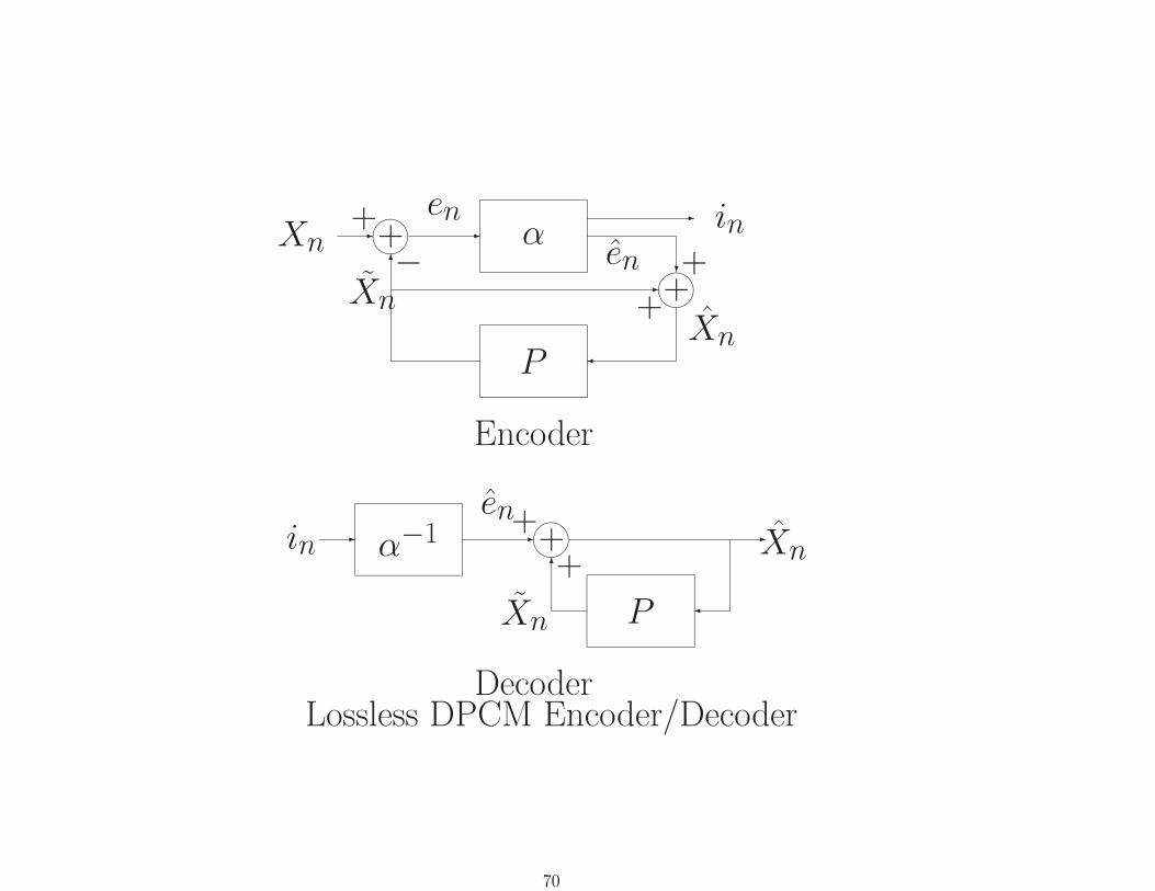
Xn -����++6

Xn−

-

enα

en

- in

����++Xn

?+-

P �

Encoder

in - α−1 -

en����+ -Xn

�P

6

Xn

++

DecoderLossless DPCM Encoder/Decoder

70

Part III: Lossy Compression

Uniform Scalar QuatizationRoundoff numbers to nearest number in discrete set.> 100 years old.

Original A/D converter was pulse coded modulation (PCM)(Oliver, Pierce, Shannon)

Uniform scalar quantization coded by binary indexes.

Mathematical “compression” since mapped analog space intodigital space.

Not practical “compression” since expanded required bandwidthgiven modulation techniques of the time.

71

Example

Speech ≈ 4 kHz BW.

Sample @ 8 kHz, Quantize to 8bpp⇒ 64 kbpsWith traditional ASK, PSK, or FSK, get about 1 bit per HzThus new BW ≈ 64 kHz, 16 times greater than original analogwaveform!!

72

Optimal Scalar QuatizationLloyd (1956)Optimize PCM by formulating as a constrained optimizationproblem

X is scalar real-valued random variable, with pdf fXQuantizer:

Encoder α : < → II is {0, 1, 2, . . . , N − 1}, or an equivalent set of binaryvectors.

Decoder β : I → <Overall Quantizer Q(x) = β(α(x))

Reproduction codebook C = {β(i); i ∈ I}

73

Problem: Given N , find the encoder α and decoder β thatminimize the average distortion (MSE)

E[(X −Q(X))2] =∫(x−Q(x))2fX(x) dx

=N∑i=1

Pr(α(X) = i))E[(X − β(i))2|α(X) = i]

An example of statistical clustering.Lloyd algorithm for optimal PCM was one of the originalclustering algorithms. (k-means, isodata, principal points)

Strong parallel between optimal quantization and statisticalalgorithms for clustering/classification/pattern recognition.

74

Idea:? Suppose the decoder β is fixed, then the optimal encoder is

α(x) = i which minimizes |x− β(i)|2

(minimum distortion encoder, nearest neighbor encoder)

? Suppose the encoder α is fixed, then the optimal decoder is

β(i) = E[X|α(X) = β(i)]

Conditional expectation is optimal nonlinear estimate.

This gives a descent algorithm for improving a code:

1. Optimize the encoder for the decoder.

2. Optimize the decoder for the encoder.

Continue until convergence.

75

General formulation: Lloyd (1957)Special case (calculus derivation) Max (1960)“Lloyd-Max Quantizer”

In general only a local optimum, sometimes global (Gaussian)

Most common techniques employ scalar quantization, butimprove performance via prediction, transforms, or other linearoperations.

Uniform simple vs. Lloyd-optimal better performance

Compromise: Companding (µ-law, A-law, etc.)

76

Caveat Optimal for fixed rate, i.e., number of quantizer levels Nis fixed. Not optimized for variable rate (variable length) codes,e.g., if fix entropy instead of N . (Entropy constrainedquantization.)

There are generalized Lloyd algorithms for designing ECQ, butthere are theoretical results (will sketch later) that show:

If the rate is large, then the quantizer solving the ECQproblem, i.e., minimizing MSE for a given entropy (henceassuming a subsequent entropy coder), is approximatelyuniform!

Thus if variable-rate coding is allowed and the rate is large,uniform quantization is nearly optimal.

77

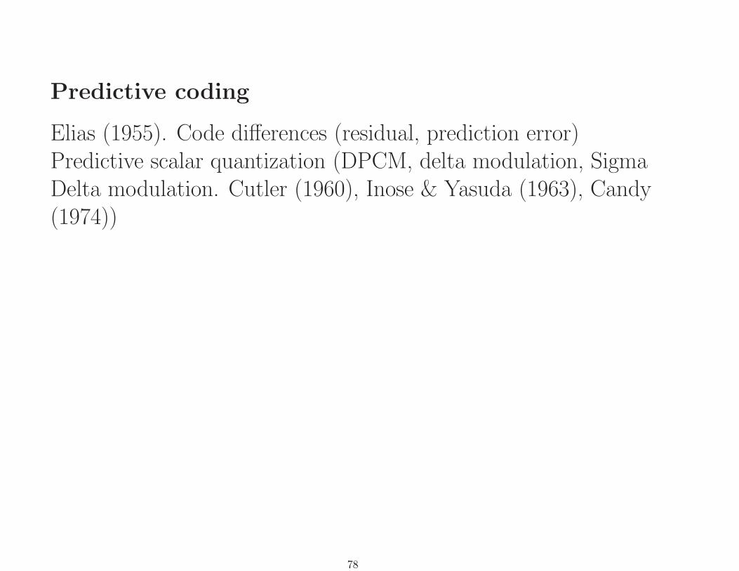
Predictive coding

Elias (1955). Code differences (residual, prediction error)Predictive scalar quantization (DPCM, delta modulation, SigmaDelta modulation. Cutler (1960), Inose & Yasuda (1963), Candy(1974))

78

Xn -����++6

Xn−

-

enQ

en

- in

����++Xn

?+-

P �

Encoder

in - Q−1 -

en����+ -Xn

�P

6

Xn

++

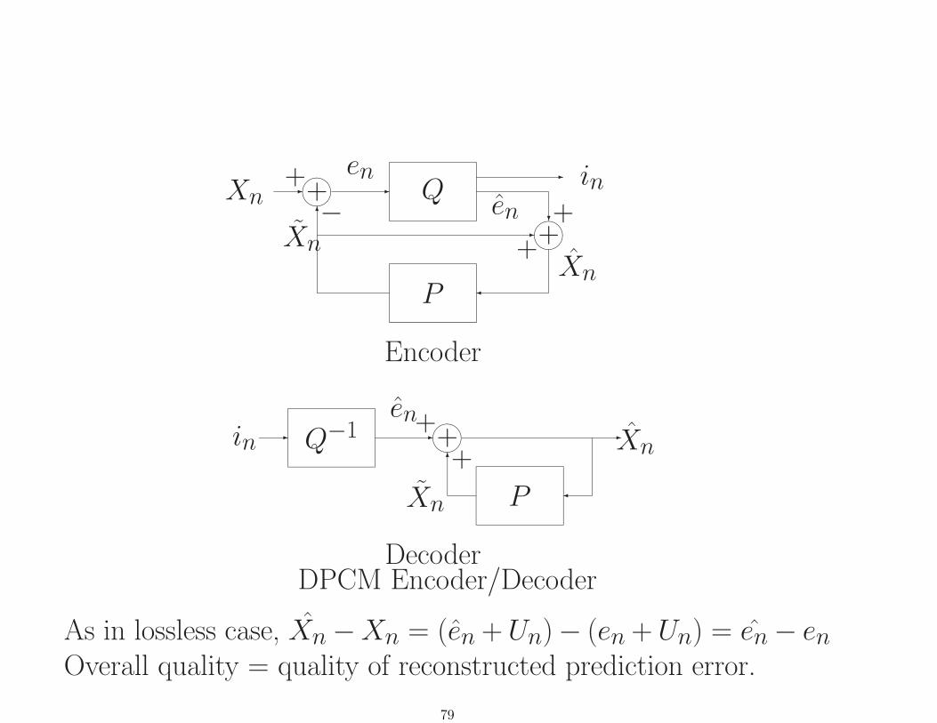
DecoderDPCM Encoder/Decoder

As in lossless case, Xn−Xn = (en +Un)− (en +Un) = en− enOverall quality = quality of reconstructed prediction error.

79

Transform Coding

Mathews and Kramer (1956)Huang, Habibi, Chen (1960s)

Dominant image coding (lossy compression) method: ITU andother standards p*64, H.261, H.263, JPEG, MPEGC-Cubed, PictureTel, CLI

80

X

X1

X2

Xk

-

-

...

-

T

Y

-

-

-

Q1

Q2

...

Qk

Y

-

-

-

T−1

-

-

...

-

X1

X2

Xk

X

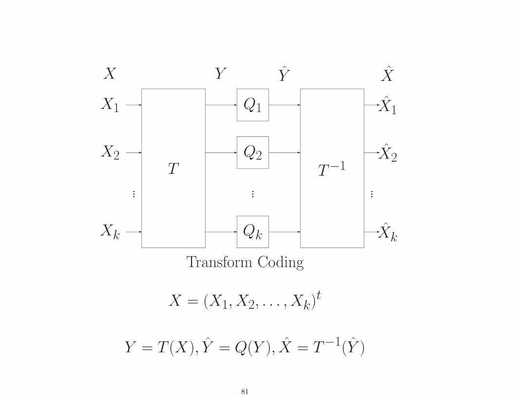
Transform Coding

X = (X1, X2, . . . , Xk)t

Y = T (X), Y = Q(Y ), X = T−1(Y )

81

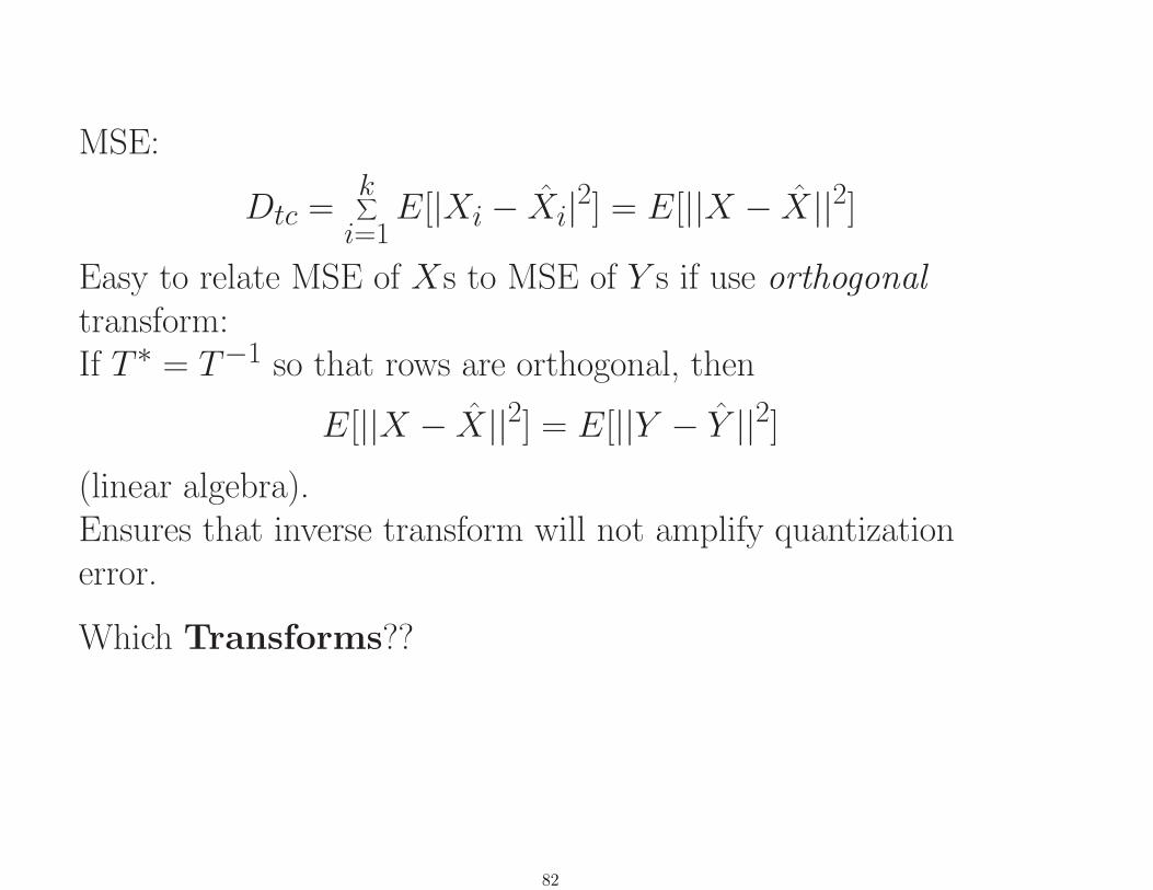
MSE:

Dtc =k∑i=1

E[|Xi − Xi|2] = E[||X − X||2]

Easy to relate MSE of Xs to MSE of Y s if use orthogonaltransform:If T ∗ = T−1 so that rows are orthogonal, then

E[||X − X||2] = E[||Y − Y ||2]

(linear algebra).Ensures that inverse transform will not amplify quantizationerror.

Which Transforms??

82

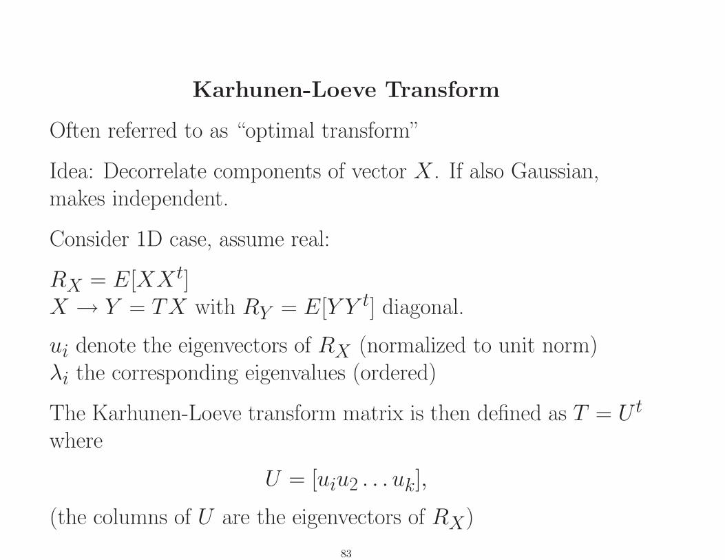
Karhunen-Loeve Transform

Often referred to as “optimal transform”

Idea: Decorrelate components of vector X . If also Gaussian,makes independent.

Consider 1D case, assume real:

RX = E[XXt]X → Y = TX with RY = E[Y Y t] diagonal.

ui denote the eigenvectors of RX (normalized to unit norm)λi the corresponding eigenvalues (ordered)

The Karhunen-Loeve transform matrix is then defined as T = Ut

where

U = [uiu2 . . . uk],

(the columns of U are the eigenvectors of RX)

83

Then

RY = E[Y Y t] = E[UtXXtU ] = UtRXU = diag(λi).

Note that the variances of the transform coefficients are theeigenvalues of the autocorrelation matrix RX .

Many other transforms, but dominant ones are discrete cosinetransform (DCT, the 800 lb gorilla) and discrete wavelettransform (DWT).

Theorems to show that if image ≈ Markovian, then DCTapproximates KL

Wavelet fans argue that wavelet transforms ≈ decorrelate widerclass of images.

Often claimed KL “optimal” for Xform codes

Only true (approximately) if high rate, optimal bit allocationamong coefficients, and Gaussian.

84

Discrete Cosine Transform

The 1-D discrete cosine transform is defined by

C(u) = α(u)N−1∑x=0

f(x) cos

(2x + 1)uπ

2N

for u = 0, 1, 2, . . . , N − 1. The inverse DCT is define by

f(x) =N−1∑u=0

α(u)C(u) cos

(2x + 1)uπ

2N

for x = 0, 1, 2, . . . , N − 1. In these equations, α is

α(u) =

√√√√ 1N for u = 0√√√√ 2N for u = 1, 2, . . . N − 1.

85

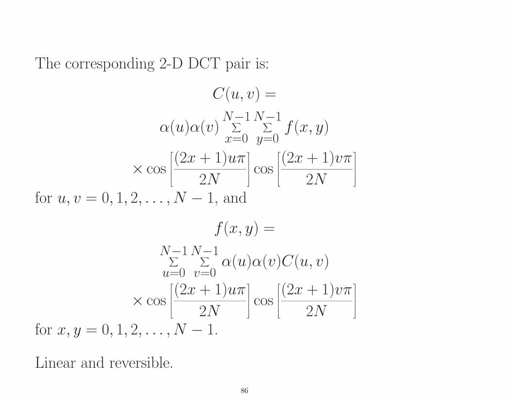
The corresponding 2-D DCT pair is:

C(u, v) =

α(u)α(v)N−1∑x=0

N−1∑y=0

f(x, y)

× cos

(2x + 1)uπ

2N

cos

(2x + 1)vπ

2N

for u, v = 0, 1, 2, . . . , N − 1, and

f(x, y) =

N−1∑u=0

N−1∑v=0

α(u)α(v)C(u, v)

× cos

(2x + 1)uπ

2N

cos

(2x + 1)vπ

2N

for x, y = 0, 1, 2, . . . , N − 1.

Linear and reversible.

86

Why DCT so important?

• real

• can be computed by an FFT

• excellent energy compaction for highly correlated data

• good approximation to Karhunen-Loeve transform for Markovbehavior and large images

Won in the open competition for an international standard.

• 1985: Joint Photographic Experts Group (JPEG) formed asan ISO/CCITT joint working group

• 6/87 12 proposals reduced to 3 in blind subjective assessmentof picture quality

• 1/88 DCT-based algorithm wins

• 92-93 JPEG becomes intl standard

87

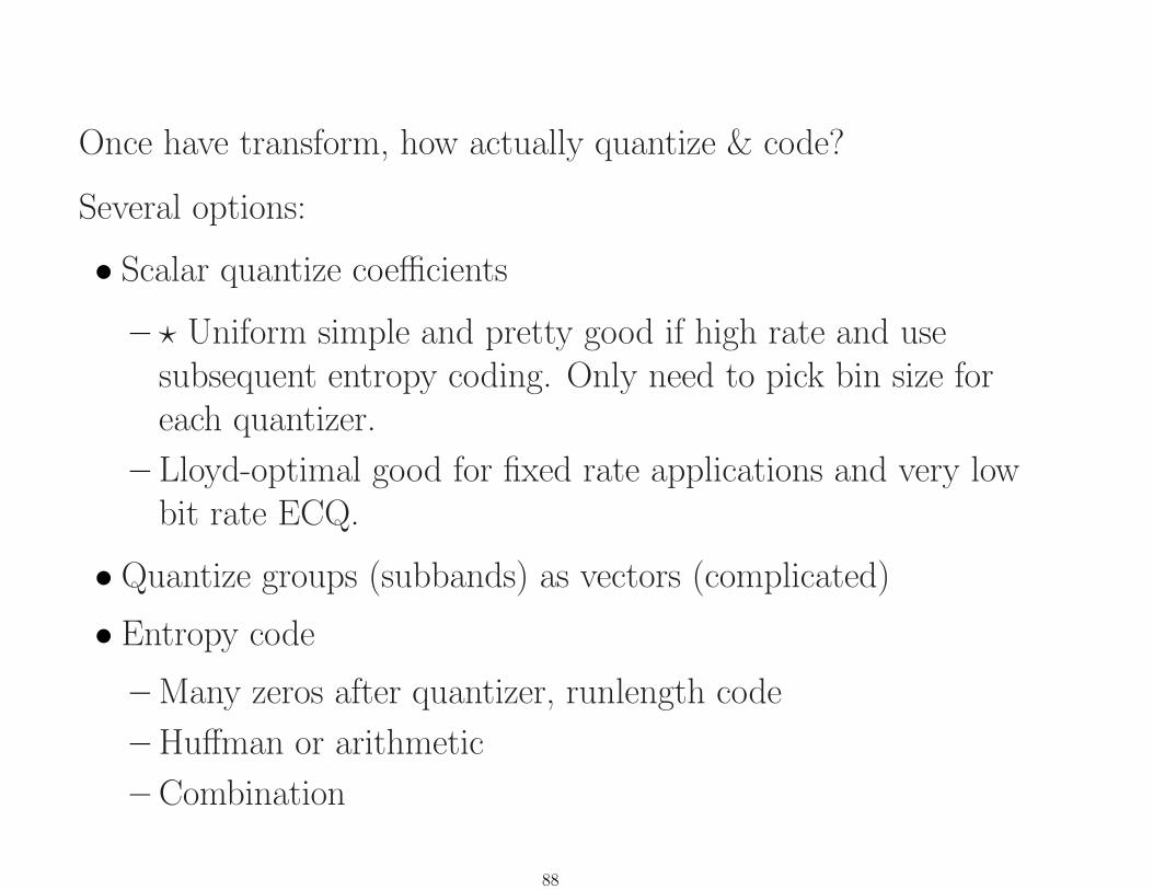
Once have transform, how actually quantize & code?

Several options:

• Scalar quantize coefficients

– ? Uniform simple and pretty good if high rate and usesubsequent entropy coding. Only need to pick bin size foreach quantizer.

– Lloyd-optimal good for fixed rate applications and very lowbit rate ECQ.

• Quantize groups (subbands) as vectors (complicated)

• Entropy code

– Many zeros after quantizer, runlength code

– Huffman or arithmetic

– Combination

88

JPEG is basically

• DCT transform coding (DCT) on 8×8 pixel blocks

• custom uniform quantizers (user-specified Quantization tables)

• runlength coding

• Huffman or arithmetic coding on (runs, levels)

DC coefficient coded separately, DPCM

Sample quantization table

89

S =

16 11 10 16 24 40 51 6112 12 14 19 26 58 60 5514 13 16 24 40 57 69 5614 17 22 29 51 87 80 6218 22 37 56 68 109 103 7724 35 55 64 81 104 113 9249 64 78 87 103 121 120 10172 92 95 98 112 100 103 99

Uniform quantization: Suppose DCT transformed 8× block is{θij}. Then quantizer output index is

lij = bθijSij

+ .5c (1)

bxc = largest integer smaller than x.

JPEG ubiquitous in WWW90

Vector quantization Quantize vectors instead of scalars.(theory in Shannon (1959), design algorithms in late 70s)

Motivation: Shannon theory⇒ better distortion/rate tradeoffsof code vectors.

Added benefit: Simple decompression in general, just tablelookup.

Problem: High encoder complexity in usual implementations.

Applications:Software based video: table lookups instead of computationPart of speech coding standards based on CELP and variations.

Basic idea: Quantize vectors instead of scalars.

As with a scalar quantizer, VQ consists of an encoder anddecoder.

91

Encoder α : A→W ⊂ {0, 1}∗ (or source encoder) α is amapping of the input vectors into a collection W of finite lengthbinary sequences.

W = channel codebook , members are channel codewords.set of binary sequences that will be stored or transmitted

W must satisfy the prefix condition

Decoder β :W → A

(table lookup)

reproduction codebook C ≡ {β(i); i ∈ W}, β(i) calledreproduction codewords or templates.

A source code or compression code for the source {Xn} consistsof a triple (α,W , β) of encoder, channel codebook, and decoder.

92

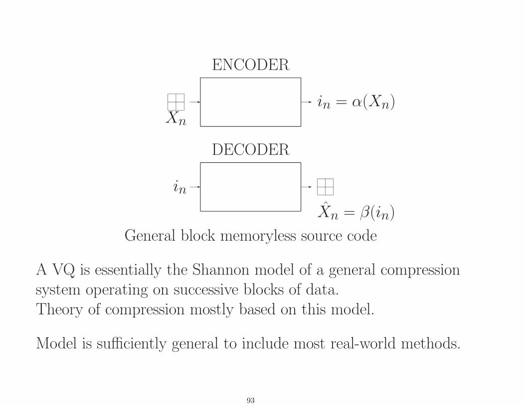
ENCODER

Xnin = α(Xn)- -

DECODER

in

Xn = β(in)

- -

General block memoryless source code

A VQ is essentially the Shannon model of a general compressionsystem operating on successive blocks of data.Theory of compression mostly based on this model.

Model is sufficiently general to include most real-world methods.

93

Performance: Rate and DistortionRate:Given an i ∈ {0, 1}∗, define

l(i) = length of binary vector i

instantaneous rate r(i) = l(i)k bits/input symbol.

Average rate R(α,W) = E[r(α(X))].

An encoder is said to be fixed length or fixed rate if all channelcodewords have the same length, i.e., if l(i) = Rk for all i ∈ W .

• Variable rate codes may require data buffering, expensive andcan overflow and underflow

• Harder to synchronize variable-rate codes. Channel bit errorscan have catastrophic effects.

94

But variable rate codes can provide superior rate/distortiontradeoffs.E.g., in image compression can use more bits for edges, fewer forflat areas. In voice compression, more bits for plosives, fewer forvowels.

Distortion

Distortion measure d(x, x) measures the distortion or lossresulting if an original input x is reproduced as x.

Mathematically: A distortion measure satisfies

d(x, x) ≥ 0

95

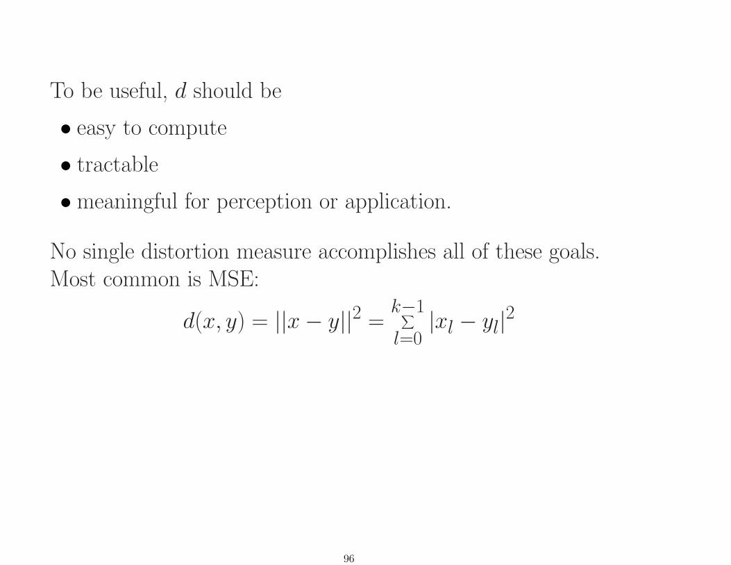
To be useful, d should be

• easy to compute

• tractable

• meaningful for perception or application.

No single distortion measure accomplishes all of these goals.Most common is MSE:

d(x, y) = ||x− y||2 =k−1∑l=0|xl − yl|2

96

Weighted or transform/weighted versions are used for perceptualcoding.

In particular: Input-weighted squared error:

d(X, X) = (X − X)∗BX(X − X),

BX positive definite.

most common BX = I , d(X, X) = ||X − X||2 (MSE)

Other measures:

Bx takes DCT and uses perceptual maskingOr weights distortion according to importance of x(Safranek and Johnson, Watson et al.)

97

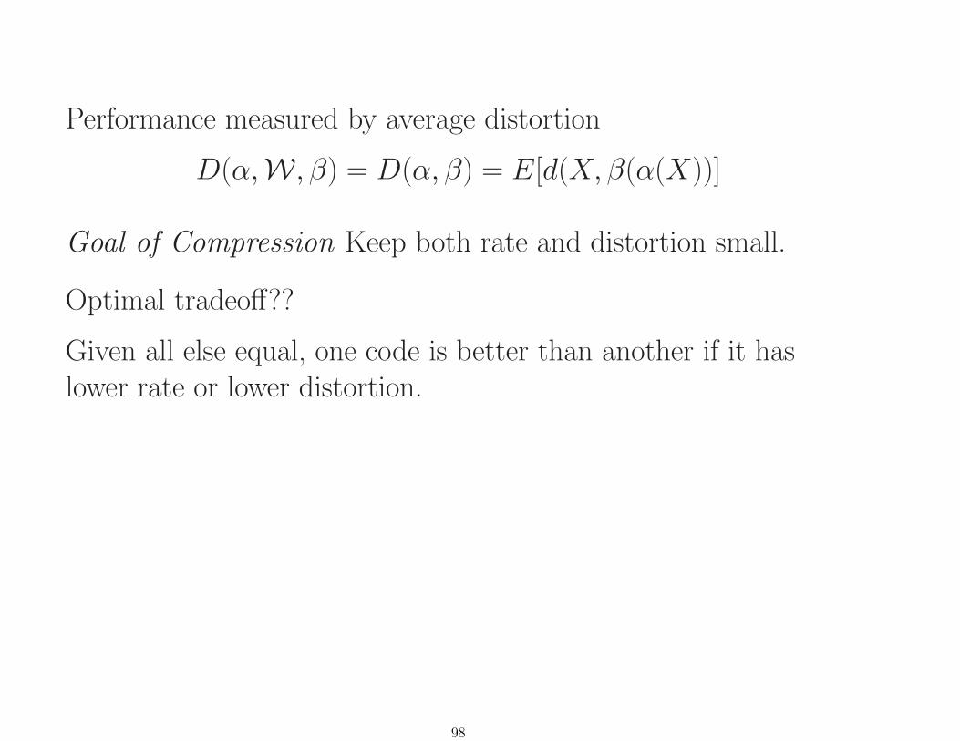
Performance measured by average distortion

D(α,W , β) = D(α, β) = E[d(X, β(α(X))]

Goal of Compression Keep both rate and distortion small.

Optimal tradeoff??

Given all else equal, one code is better than another if it haslower rate or lower distortion.

98

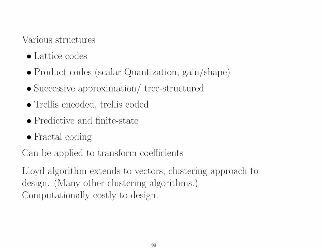
Various structures

• Lattice codes

• Product codes (scalar Quantization, gain/shape)

• Successive approximation/ tree-structured

• Trellis encoded, trellis coded

• Predictive and finite-state

• Fractal coding

Can be applied to transform coefficients

Lloyd algorithm extends to vectors, clustering approach todesign. (Many other clustering algorithms.)Computationally costly to design.

99

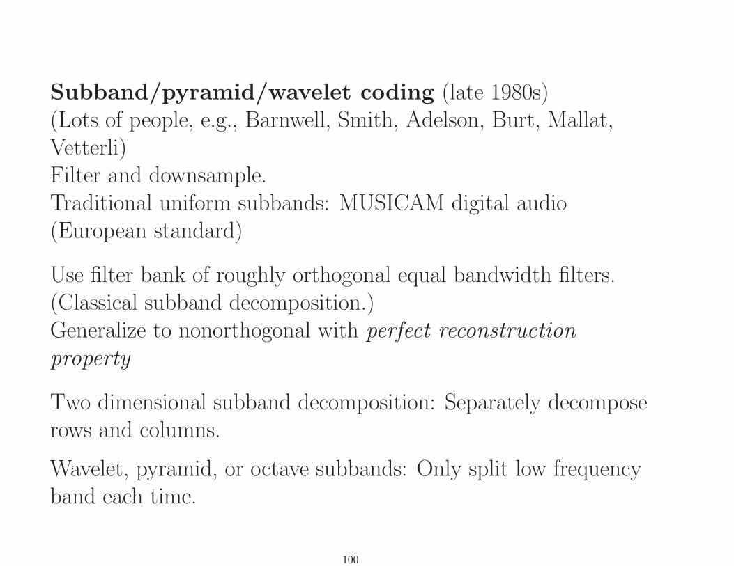
Subband/pyramid/wavelet coding (late 1980s)(Lots of people, e.g., Barnwell, Smith, Adelson, Burt, Mallat,Vetterli)Filter and downsample.Traditional uniform subbands: MUSICAM digital audio(European standard)

Use filter bank of roughly orthogonal equal bandwidth filters.(Classical subband decomposition.)Generalize to nonorthogonal with perfect reconstructionproperty

Two dimensional subband decomposition: Separately decomposerows and columns.

Wavelet, pyramid, or octave subbands: Only split low frequencyband each time.

100

-

-

-

-Xn

HM

...

H2

H1

-

-

-

XMn

X2n

X1n

↓M

...

↓M

↓M

-

-

-

YMk

Y2k

Y1k

QM

...

Q2

Q1

-

-

-

YMk

Y2k

Y1k

↑M

...

↑M

↑M

-

-

-

XMn

X2n

X1n

HM

...

H2

H1

XMn

X2n

X1n

6

-?

����+ -Xn

101

x(n)

H1(n)

H0(n)

?

?

2

2

H1(n)

H0(n)

H1(n)

H0(n)

?

?

?

?

2

2

2

2 LL

LH

HL

HH

One stage of subband decomposition with 2-D separable filters

102

LL

LH

HL

HH 6

6

6

6

2

2

2

2

G1(n)

G0(n)

G1(n)

G0(n)

6

6

2

2

G1(n)

G0(n)

x(n)

One stage of subband reconstruction with 2-D separable filters

103

(a) (b) (c)

(a) Two stages of uniform decomposition leading to 16 uniformsubbands, (b) Three stages of pyramidal decomposition, leading

to 10 octave-band subbands, (c) a wavelet packet

For each subband in an image (except the very lowest one, andthe three highest ones), each coefficient A is related to exactly 4coefficients in the next higher band.

104

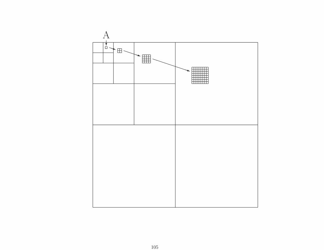
A?PPq PPPPPq

PPPPPPPPPPq

105

LenadecomposedNote:multiresolution

106

Parent-descendants

107

Question is then: How code?

I.e., how quantize wavelet coefficients and then lossy code them?

Early attempts used traditional (JPEG-like & VQ) techniques.Not impressive performance.

Breakthrough came with Knowles and Shapiro (1993):Embedded zerotree coding.

108

Idea: Coefficients have a tree structure, high frequency waveletpixels are descended from low frequency pixels.

If a low frequency pixel has low energy (and hence will bequantized into zero), then the same will likely be true for itsdescendents.⇒ zerotree encoding

Successively send bits describing higher energy coefficients togreater accuracy.

Additional bits describe most important coefficients withincreasing accuracy and less important coefficients when theirmagnitude becomes significant.

109

Variations:

• SPHIT algorithm of Said and Pearlman. Optimally trade offrate and distortion. Lower complexity, better performance.

• CREW algorithm of RICOH. Similar to SPHIT, but usesinteger arithmetic and codes to lossless.

• Others: better handling of space/frequency correlation ormore careful modeling/adaptation, but more complex:Xiong, Ramchandran, Orchard, Joshi, Jafarkani, Kasner,Fischer, Farvardin, Marcellin, Bamberger, Lopresto

Alternative: Stack-run coding (Villasenor) Simple runlengthcoding (Golomb-Rice codes) of separate subbands. Slightlyinferior performance to SPHIT, but better than Shapiro andmuch lower complexity.See Villasenor’s web site for comparisons.

110

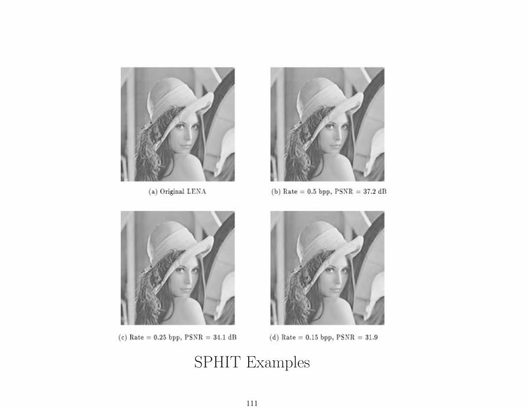
SPHIT Examples

111

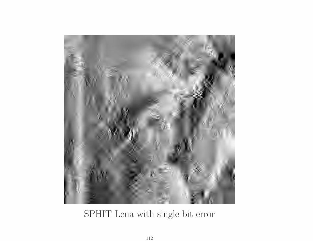
SPHIT Lena with single bit error

112

Packetizable zerotree coder,53-byte packets, 10PSNR=27.7dB

(P. Cosman, UCSD)

113

“Second Generation” CodesModel-based coding. Enormous compression reported, but needa Cray to compress. Likely to become more important.

Idea: Typically segment or identify objects/textures/backgroundwithin image, apply custom compression to each.EPFL, T. Reed (UCD), X. Wu

114

Model-based VQ: LPC

Very different methods used for low-rate speech. Many are basedon classic LPC or Parcor speech compression

Itakura and Saito, Atal and Shroeder, Markel and (A.H.) Gray

First very low bit rate speech coding based on sophisticated SP,implementable in DSP chips.Speak and Spell, TINTT, Bell, TI and Signal Technology

Model short speech segment x (≈ 25− 50ms) by autoregressiveprocess (all-pole) σ/A(z) with

A(z) = 1 +M∑k=1

akz−k.

115

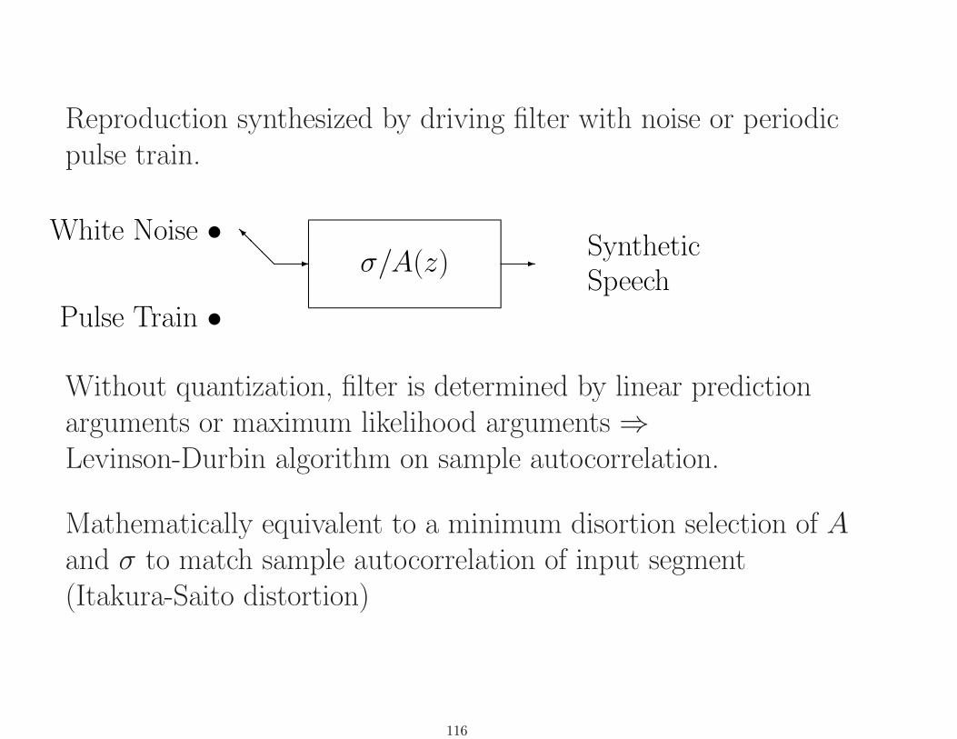
Reproduction synthesized by driving filter with noise or periodicpulse train.

White Noise •

Pulse Train •

-@@@I

σ/A(z) -SyntheticSpeech

Without quantization, filter is determined by linear predictionarguments or maximum likelihood arguments⇒Levinson-Durbin algorithm on sample autocorrelation.

Mathematically equivalent to a minimum disortion selection of Aand σ to match sample autocorrelation of input segment(Itakura-Saito distortion)

116

Parameters quantized as scalars or vectors (LPC-VQ).Several parameter vectors possible:

• reflection coefficients

• autocorrelation coefficients

• inverse filter coefficients

• cepstrum

• line spectral pairs (LSP)

Mathematically equivalent when no quantization,but quantization errors effect each differently.

117

Hybrid Model + Closed Loop ResidualCELP

(Inverted RELP, modern version of analysis-by-synthesis)

Codebook for residuals. Given input vector, find residualcodeword that produces best closed loop match out of LPC (orLPC-VQ) to original input.

Effectively produces a waveform codebook for searching bypassing residual codewords through model linear filter.

Stewart et al. (1981, 1982), Shroeder and Atal (1984, 1985)

118

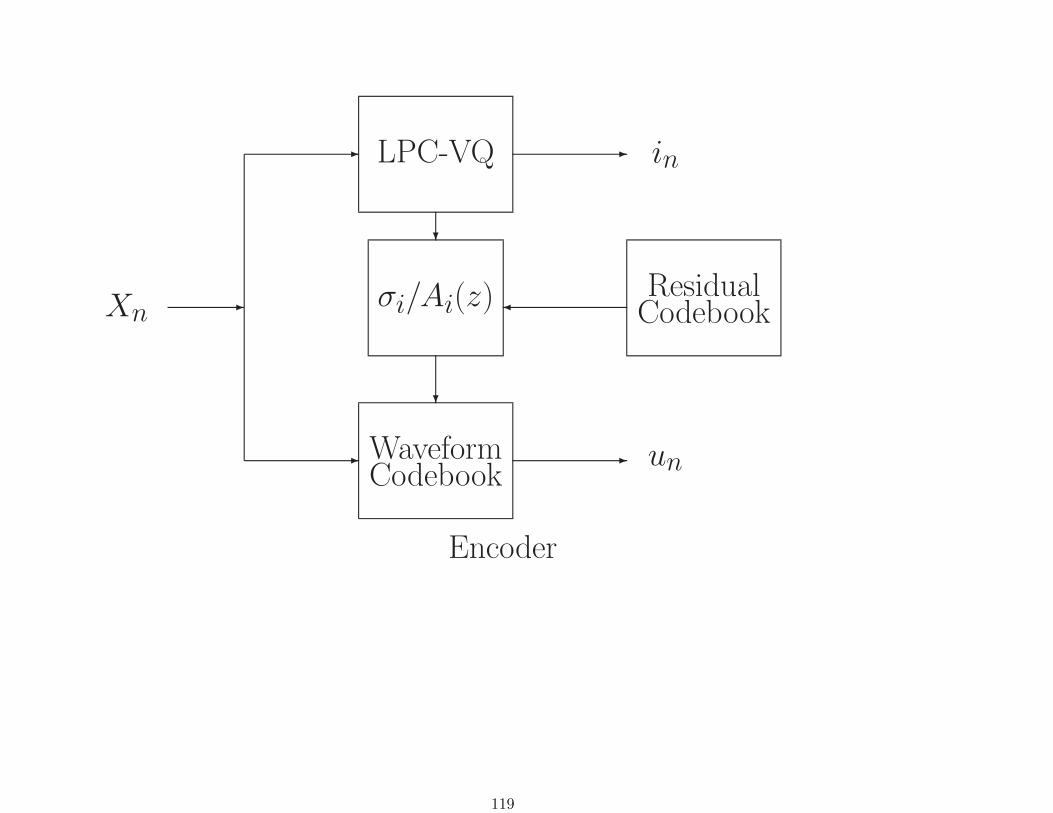
Xn -

-

-

LPC-VQ - in

?

σi/Ai(z)

?

WaveformCodebook

- un

�Residual

Codebook

Encoder

119

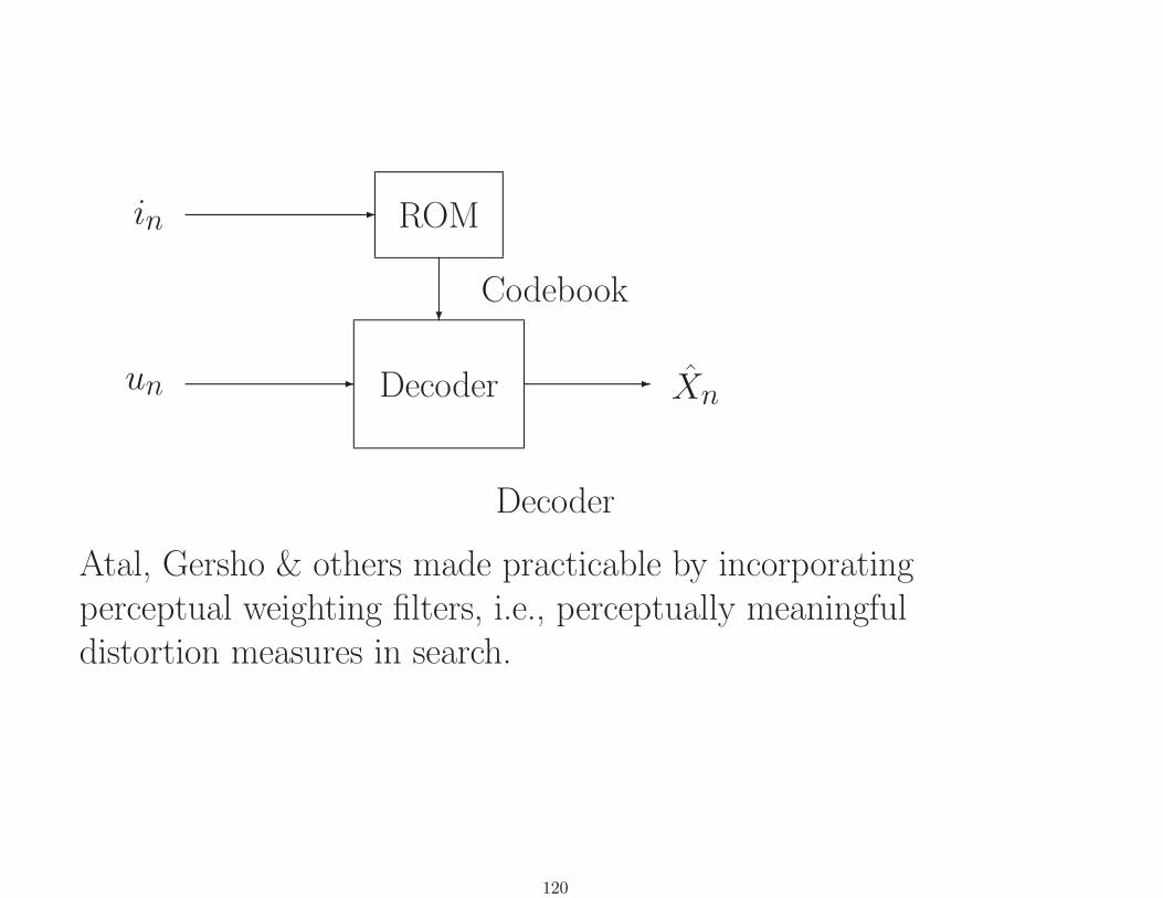
un

in

-

- ROM

?

Decoder

Codebook

- Xn

Decoder

Atal, Gersho & others made practicable by incorporatingperceptual weighting filters, i.e., perceptually meaningfuldistortion measures in search.

120

Measuring Quality in

Lossy Compressed Images

Digitization, digital acquisition, compression, and DSP (even“enhancement”) change content.Allegedly for the better, but how prove quality or utilityequivalent or superior?

SNR Can be useful for screening among algorithms and tellssomething about relative performance.Possibly sufficient for “substantial equivalence” of minorvariation.

Subjective Ratings Ask users to rate the “quality” of theimage on a scale of 1 — 5.

121

Diagnostic Accuracy Simulate clinical application: screeningor diagnosis.Statistical analysis to test hypothesis that “image type A asgood as or better than image type B” for specific tasks.

122

Selected Standards

• ITU (International Telecommunications Union)

– telecommunications (telephony, teleconferencing, . . . )

– low-delay two-way communications

– recommendations; nations are members

• ISO (International Standards Organization)

– computer information technology

– asymmetric one-way communications

– standards; standards bodies are members

123

ITU “p× 64” recommendations

(1990)

• for video telephony and video conferencing at ISDN rates (p×

64 kb/s)

– H.261 video coding at p× 64 kb/s

– G.711 audio coding at p× 64 kb/s

(8kHz µ-law PCM)

– H.221 multiplexing, H.242 control

– H.320 capability negotiation

124

ITU, ISO ‘JBIG (Joint Bi-level Experts Group)

(1993)

Transmission storage of binary images at multiple spatial

resolutions, multiple amplitude resolutions

Context adaptive arithmetic coding

125

ITU “LBC” recommendations

(1997)

• for video telephony at modem rates

(14.4 – 28.8 Kb/s and higher)

– H.263 video coding at p× 64 kb/s

– G.723 audio coding at 6.3 kb/s

(ACELP)

– H.224 multiplexing, H.245 control

– H.324 capability negotiation

126

ISO “MPEG-1” standard

(1992)

• for entertainment video ad CDROM rates

(≈ 1.5 Mb/s)

– video coding at ≈ 1.2Mb/s

– audio coding at ≈ 64Kb/s per channel (stereo)

– systems (multiplexing, buffer management,

synchronization, control, capability negotiation)

127

Frame sequence: I B B P B B P B B I

I= Intraframe coding ( a la JPEG)

P= Predictive coding (motion estimation)

B= Bidirectional prediction (forward or backward)

Motion estimation: Predict macroblocks by matching luminance

for minimum MSE, code resulting residual by ≈ JPEG

128

ISO “MPEG-2” standard

(1994)

• for digital mastering and distribution of entertainment video

at BISDN rates

(≈ 1.5 – 10 Mb/s and higher)

– video coding at ≈ 1.5 – 10 Mb/s

– audio coding at ≈ 64Kb/s per channel (up to 5 channels)

– systems (multiplexing, buffer management,

synchronization, control, capability negotiation)

129

ISO “MPEG-4” standard

(1997)

• for interactive information access from computers, set-top

boxes, mobile units

(≈ 10 Kb/s – 1.5 Mb/s)

Intersection of computers (interactivity), entertainment (A/V

data), and telecommunications (networks, including wireless).

130

Applications

• Interactive information access

– home shopping, interactive instruction manuals, remote

eductation, travel brochures

•Multiuser communication

– conferencing with shared resources, chat rooms, games

– Editing and recomposition; search

131

• Scalable to channel BW and decoder capabilities

• Error resilience

• Coding of arbitrarily shaped regions

• Composition of Visual Objects and Audio Objects

132

Part IV: Optimal Compression

A survey of some theory and implications and applications

General Goal: Given the signal and the channel, find an

encoder and decoder which give the “best possible”

reconstruction.

To formulate as precise problem, need

• probabilistic descriptions of signal and channel

(parametric model or sample training data)

133

• possible structural constraints on form of codes

(block, sliding block, recursive)

• quantifiable notion of what “good” or “bad” reconstruction is

(MSE, Pe)

Mathematical: Quantify what “best” or optimal achievable

performance is.

134

History

1948 Shannon published “A Mathematical Theory of

Communication”

Followed in 1959 by “Coding theorems for a discrete source with

a fidelity criterion”

Probability theory, random process theory, and ergodic theory⇒

fundamental theoretical limits to achievable performance:

135

Given probabilistic model of an information source and channel

(for storage or transmission),

how reliably can the source signals be communicated to a

receiver through a channel?

Channel characterized by Shannon channel capacity C which

indicates how fast information can be reliably sent though it,

possibly subject to constraints

136

Information source characterized by Shannon distortion-rate

function D(R), the minimum average distortion achievable

when communicating at a rate R

Dual: rate-distortion function R(D), the minimum average

rate achievable when communicating at a rate D.

Both quantities are defined as optimizations involving

information measures and distortion measures such as mean

squared error or signal-to-noise ratios.

137

Shannon proved coding theorems showing these information

theoretic quantities were equivalent to the corresponding

operational quantities.

In particular: joint source/channel coding theorem:

Joint Source/Channel Coding Theorem

If you transmit information about a source with DRF D(R) over

a channel with capacity C, then you will have average distortion

at least D(C). (Negative theorem)

138

Furthermore, if complexity and cost and delay are no problem to

you, then you can get as close to D(C) as you would like by

suitable coding (Positive theorem).

Hitch: Codes may be extremely complex with large delay.

Shannon’s distortion rate theory: Fixed R, asymptotically large

k.

139

Alternative: Bennett/Zador/Gersho asymptotic quantization

theory; fixed k, asymptotically large R.

Bennett(1948), Zador (1963), Gersho (1979), Neuhoff and Na

(1995)

What does theory have to do with the real world?

• Benchmark for comparison for real communication systems.

• Has led to specific design methods and code structures.

Impossible to do better than Shannon’s bounds (unless you cheat

or have inaccurate model).

140

Theory does not include many practically important issues, e.g.:

• Coding delay

• Complexity

• Robustness to source variations

• Effects of channel errors

Over the years, methods evolved to come close to these limits in

many applications.

141

InputSignal

- Encoder - Channel - Decoder -ReconstructedSignal

Famous Figure 1

Classic Shannon model of point-to-point communication system

General Goal: Given the signal and the channel, find

encoder/decoder which give “best possible” reconstruction.

142

To formulate as precise problem, need

• probabilistic descriptions of signal and channel

(parametric model or sample training data)

• possible structural constraints on form of codes

(block, sliding block, recursive)

• quantifiable notion of “good” or “bad”: distortion

Typical assumptions:

143

• Signal is discrete time or space (e.g., already sampled),

modeled as a vector-valued random process {Xn}, common

distribution PX . Noiseless channel.

• Code maps blocks or vectors of input data into binary strings,

i.e., a VQ (α,W , β)

• Performance measured by D(α, β) = E[d(X, β(α(X))],

R(α,W) = E(r(X))

(Theory can be extended to other structures, e.g., sliding-block

codes, trellis and tree codes, finite-state codes)

144

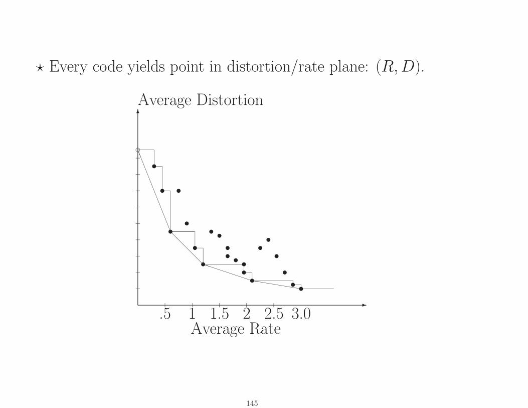
? Every code yields point in distortion/rate plane: (R,D).

-

6

Average Distortion

.5 1 1.5 2 2.5 3.0Average Rate

uuu

u

e

hhhhhhhhP

PPPP

PPP@

@@

@@LLLLLLLLLLLLL

uuuuu

uuuuuuuu

uuu

u

145

Interested in undominated points in D-R plane: For given rate

(distortion) want smallest possible distortion (rate)⇔ optimal

codes

Optimization problem:

• Given R, what is smallest possible D?

• Given D, what is smallest possible R?

• ? Lagrangian formulation: What is smallest possible D + λR?

146

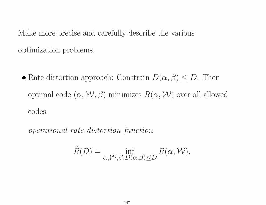
Make more precise and carefully describe the various

optimization problems.

• Rate-distortion approach: Constrain D(α, β) ≤ D. Then

optimal code (α,W , β) minimizes R(α,W) over all allowed

codes.

operational rate-distortion function

R(D) = infα,W ,β:D(α,β)≤D

R(α,W).

147

• Distortion-rate approach: Constrain R(α,W) ≤ R. Then

optimal code (α,W , β) minimizes D(α, β) over all allowed

codes.

operational distortion-rate function

D(R) = infα,W ,β:R(α,W)≤R

D(α, β).

148

• Lagrangian approach: Fix Lagrangian multiplier λ.

Optimal code (α,W , β) minimizes

Jλ(α,W , β) = D(α, β) + λR(α,W)

over all allowed codes.

operational Lagrangian distortion function

Jλ = infα,W ,β

Eρλ(X, β(α(X))) =

infα,W ,β

[D(α, β) + λR(α,W)].

First two problems are duals, all three are equivalent. E.g.,

Lagrangian approach yields R-D for some D or D-R for some R.

149

Lagrangian approach effectively uncostrained minimization of

modified distortion Jλ = Eρλ(X,α(X)) where

ρλ(X,α(X)) = d(X, β(α(X)) + λl(α(X))

Note: Lagrangian formulation has recently proved useful for rate

control in video, optimize distortion + λ rate.

Usually wish to optimize over constrained subset of

computationally reasonable codes, or implementable codes.

150

Example: fixed rate codes

Require all words inW = range space ofW to have equal length.

Then r(X) constant and problem simplified.

Eases buffering requirments when use fixed-rate transmission

media, Eases effects of channel errors

Lagrangian approach⇔ distortion-rate approach for fixed R.

151

Optimalility Properties and Quantizer Design

Extreme Points

Can actually find global optima for two extreme points:

λ→ 0: all of the emphasis on distortion

force 0 average distortion

Minimize rate only as an afterthought.

(0, R) 0 distortion, corresponds to lossless codes

152

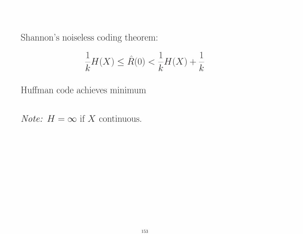
Shannon’s noiseless coding theorem:

1

kH(X) ≤ R(0) <

1

kH(X) +

1

k

Huffman code achieves minimum

Note: H =∞ if X continuous.

153

λ→∞

All emphasis on rate, force 0 average rate

minimize distortion as an afterthought.

(D, 0): 0 rate, no bits communicated.

Optimal peformance:

D(0) = infy∈A

E[d(X, y)].

centroid

154

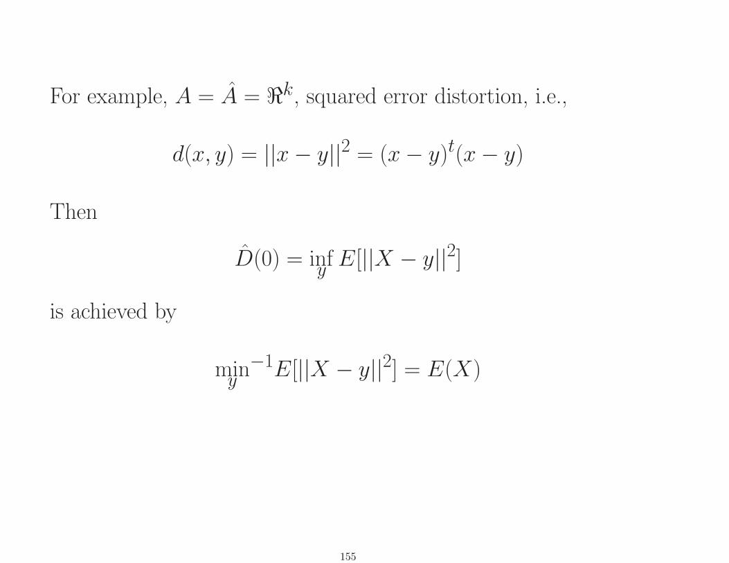
For example, A = A = <k, squared error distortion, i.e.,

d(x, y) = ||x− y||2 = (x− y)t(x− y)

Then

D(0) = infyE[||X − y||2]

is achieved by

miny−1E[||X − y||2] = E(X)

155

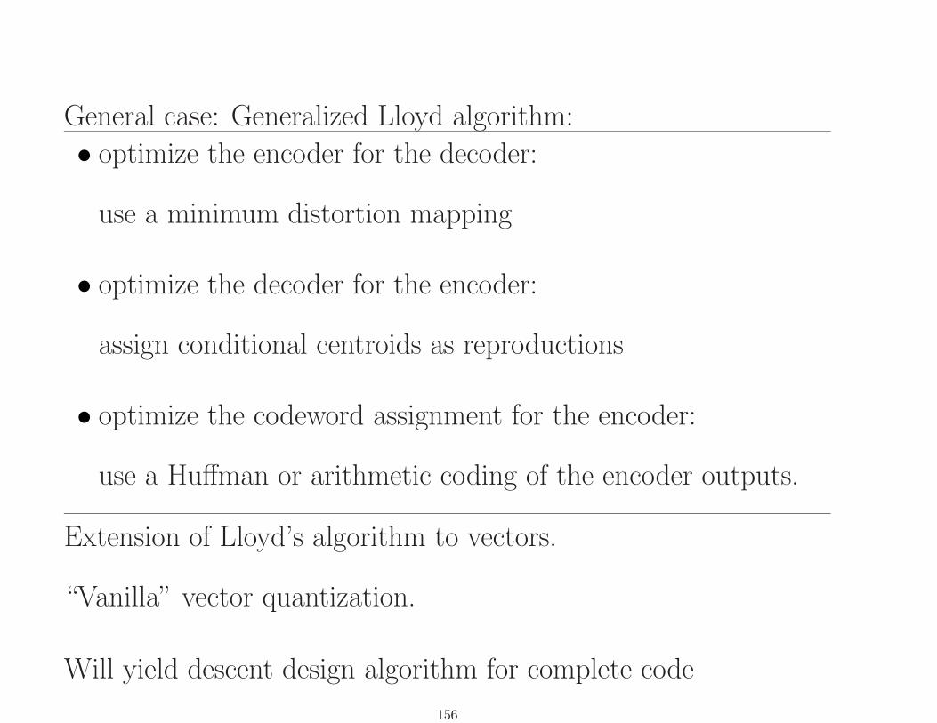
General case: Generalized Lloyd algorithm:

• optimize the encoder for the decoder:

use a minimum distortion mapping

• optimize the decoder for the encoder:

assign conditional centroids as reproductions

• optimize the codeword assignment for the encoder:

use a Huffman or arithmetic coding of the encoder outputs.

Extension of Lloyd’s algorithm to vectors.

“Vanilla” vector quantization.

Will yield descent design algorithm for complete code

156

Hierarchical (Table Lookup) VQ

(Chang et al. (1985 Globecom)) Vector quantization can involve

significant computation at encoder because of searching, but

decoder is simple table lookup.

Can also make encoder table lookup and hence trade

computation for memory if use hierarchical table lookup encoder:

157

︸ ︷︷ ︸︸ ︷︷ ︸︸ ︷︷ ︸︸ ︷︷ ︸↓ ↓ ↓ ↓

2D VQ8 bpp

︸ ︷︷ ︸︸ ︷︷ ︸↓ ↓

4 bpp4D VQ

︸ ︷︷ ︸↓

2 bpp8D VQ

1 bpp

Each arrow is implemented as a table lookup having 65536

possible input indexes and 256 possible output indexes. The

table is populated by an off-line minimum distortion search.

158

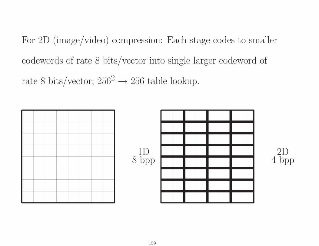
For 2D (image/video) compression: Each stage codes to smaller

codewords of rate 8 bits/vector into single larger codeword of

rate 8 bits/vector; 2562→ 256 table lookup.

1D8 bpp

2D4 bpp

159

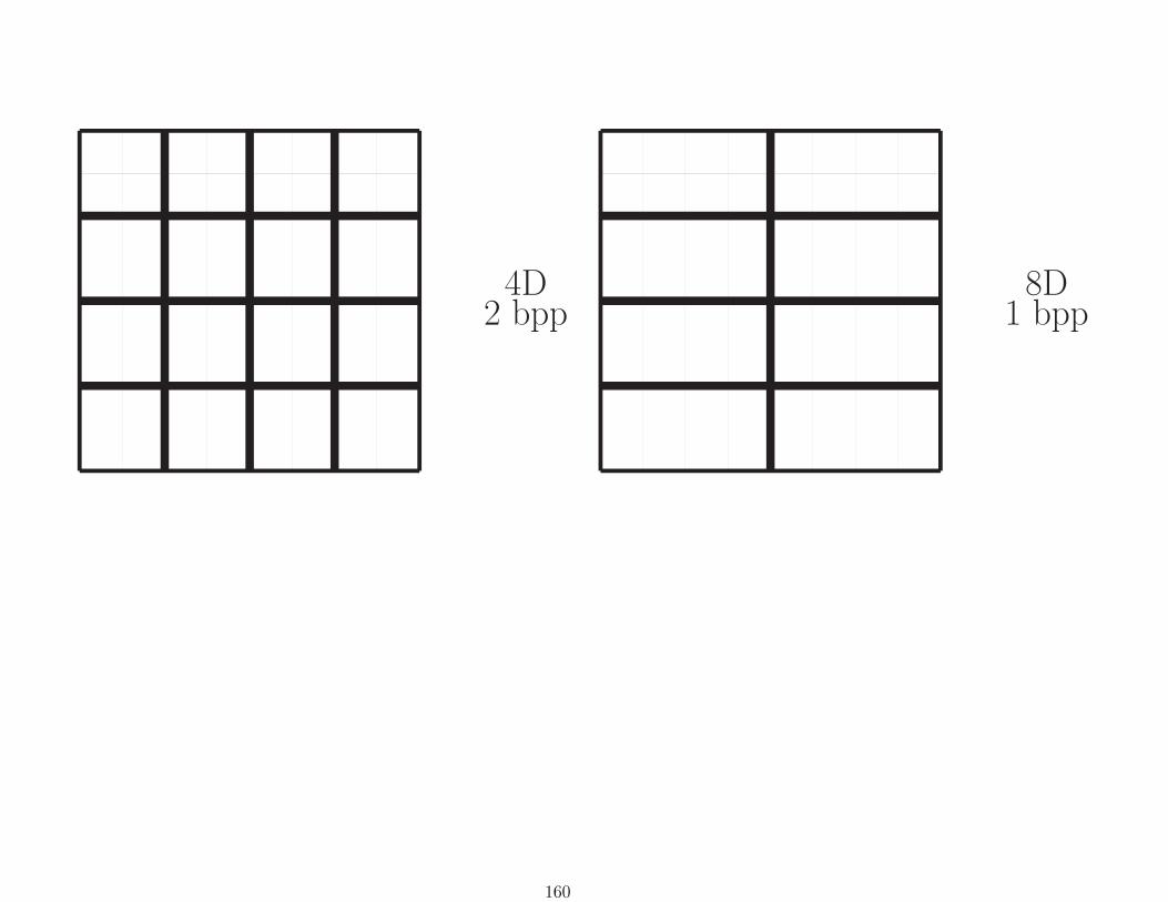
4D2 bpp

8D1 bpp

160

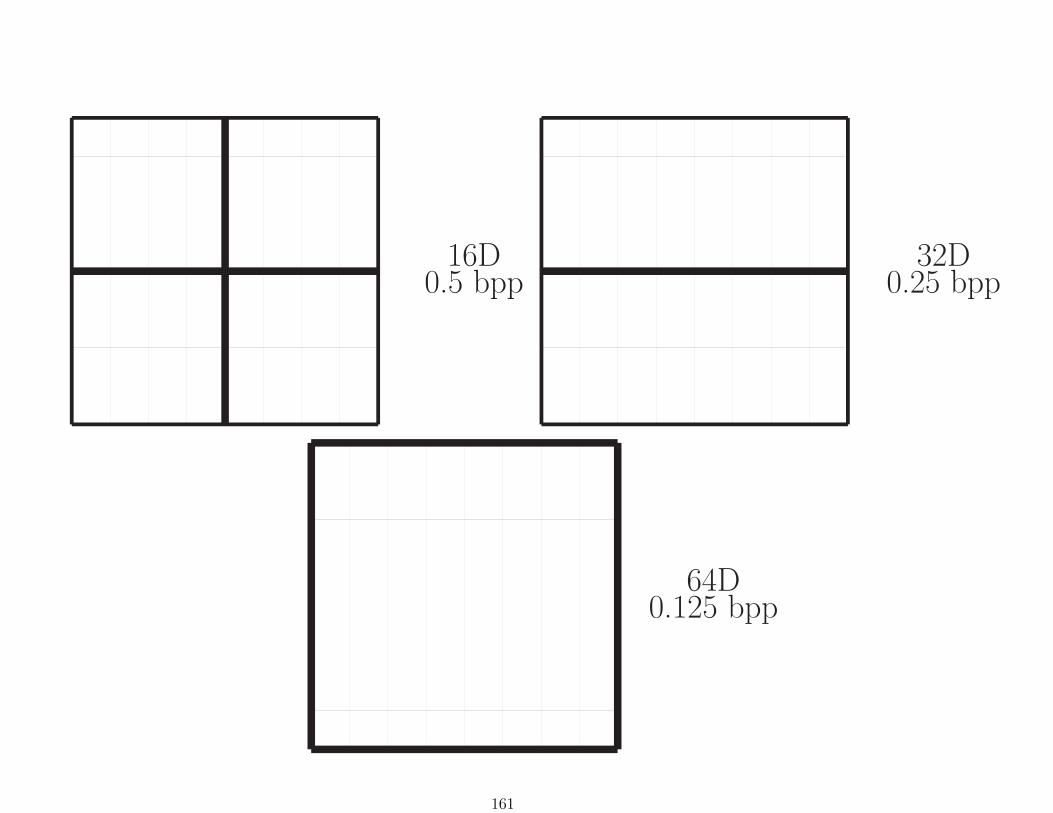
16D0.5 bpp

32D0.25 bpp

64D0.125 bpp

161

Can combine with transform coding and perceptual distortion

measures to improve.

(Chou, Vishwanath, Chaddha)

Yields very fast nearly computation-free compression.

162

Increasing Dimension

X = Xk, k allowed to vary.

Can define optima for increasing dimensions:

Dk(R), Rk(D), and Jλ,k

Quantities are subadditive & can define asymptotic optimal

performance

¯D(R) = inf

kDk(R) = lim

k→∞Dk(R)

¯R(D) = inf

kRk(D) = lim

k→∞Rk(D)

163

¯Jλ = inf

kJλ,k = lim

k→∞Jλ,k.

Shannon coding theorems relate these operationally optimal

performances (impossible to compute) to information theoretic

minimizations.

¯D(R) = D(R),

¯R(D) = R(D)

i.e., operational DRF (RDF) = Shannon DRF (RDF)

Need some definitions to define Shannon DRF.

164

Average mutual information between two discrete random

variables X and Y is

I(X ;Y ) = H(X) + H(Y )−H(X, Y ) =

∑x,y

Pr(X = x, Y = y) log2Pr(X = x, Y = y)

Pr(X = x) Pr(Y = y)

Definition extends to continuous alphabets by maximizing over

all quantized versions:

I(X ;Y ) = supα1,α2

I(α1(X);α2(Y ))

165

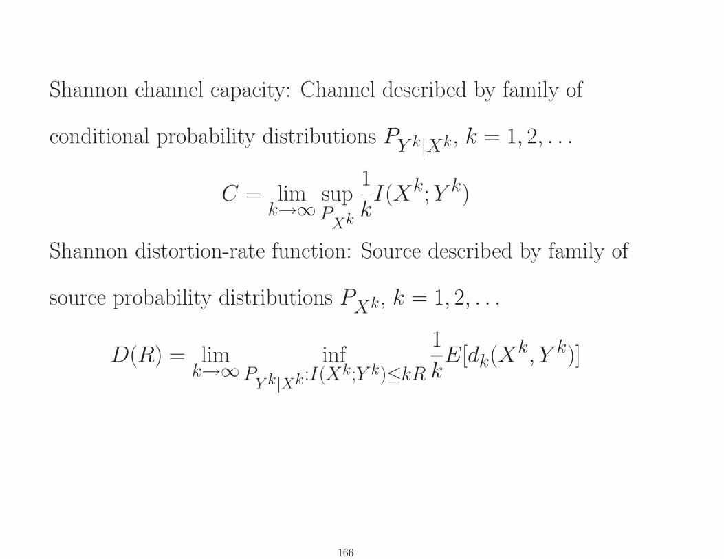
Shannon channel capacity: Channel described by family of

conditional probability distributions PY k|Xk, k = 1, 2, . . .

C = limk→∞

supPXk

1

kI(Xk;Y k)

Shannon distortion-rate function: Source described by family of

source probability distributions PXk, k = 1, 2, . . .

D(R) = limk→∞

infPY k|Xk :I(Xk;Y k)≤kR

1

kE[dk(Xk, Y k)]

166

Lagrangian a bit more complicated, equals D + λR, where

D = D(R) at point where λ is the magnitude of the slope of the

DRF.

167

Shannon’s distortion rate-theory is asymptotic in that its

positive results are for a fixed rate R and asymptotically large

block size k (and hence large coding delay)

Another approach: Bennett/Zador/Gersho asymptotic

quantization theory.

Fixed k, asymptotically large R.

High rate or low distortion theory.

Theories consistent when both R and k asymptotically large.

But keep in mind: the real world is not asymptopia!

168

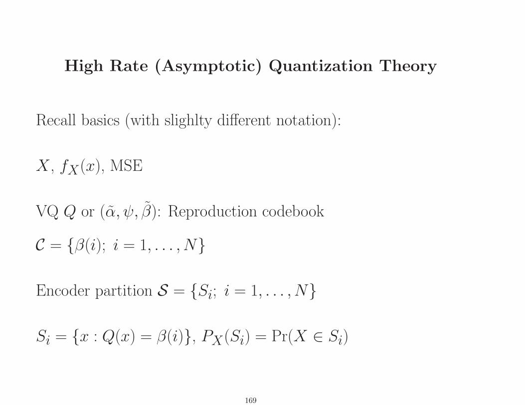
High Rate (Asymptotic) Quantization Theory

Recall basics (with slighlty different notation):

X , fX(x), MSE

VQ Q or (α, ψ, β): Reproduction codebook

C = {β(i); i = 1, . . . , N}

Encoder partition S = {Si; i = 1, . . . , N}

Si = {x : Q(x) = β(i)}, PX(Si) = Pr(X ∈ Si)

169

Average distortion:

D(Q) =1

kE[||X −Q(X)||2]

=1

k

N∑i=1

∫Si ||x− β(i)||2fX(x) dx

Average rate: Fixed rate code: R(Q) = k−1 logN

Variable rate code:

R(Q) = Hk(X) = −1k

∑Ni=1PX(Si) logPX(Si)

As in ECVQ, constraining entropy effectively constraining

average length.

170

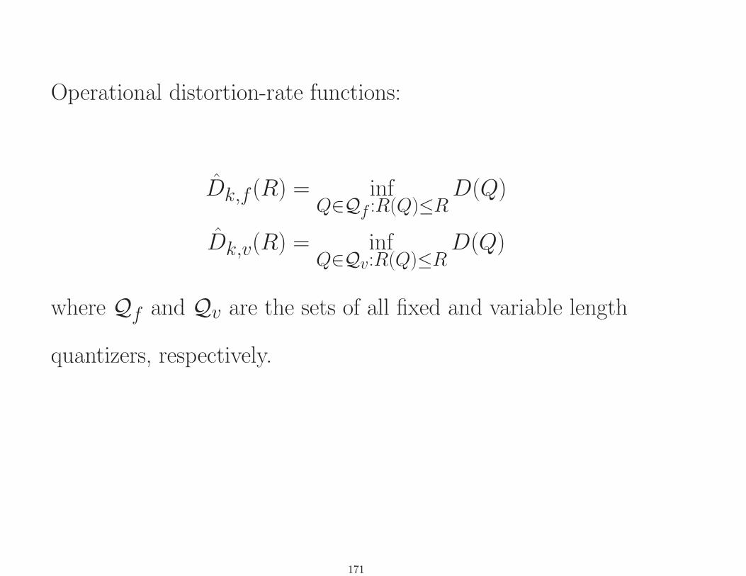
Operational distortion-rate functions:

Dk,f (R) = infQ∈Qf :R(Q)≤R

D(Q)

Dk,v(R) = infQ∈Qv:R(Q)≤R

D(Q)

where Qf and Qv are the sets of all fixed and variable length

quantizers, respectively.

171

Bennett assumptions:

• N is very large

• fX is smooth (so that Riemann sums approach Riemann

integrals and mean value theorem of calculus applies)

• The total overload distortion is negligible.

• The volumes of all bounded cells are tiny.

• The reproduction codewords are the Lloyd centroids of their

cell.

172

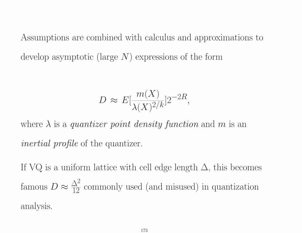
Assumptions are combined with calculus and approximations to

develop asymptotic (large N) expressions of the form

D ≈ E[m(X)

λ(X)2/k]2−2R,

where λ is a quantizer point density function and m is an

inertial profile of the quantizer.

If VQ is a uniform lattice with cell edge length ∆, this becomes

famous D ≈ ∆2

12 commonly used (and misused) in quantization

analysis.

173

Result has many applications:

Can use to evaluate scalar and vector quantizers, transform

coders, tree-structured quantizers. Can provide bounds.

Can show, for example, that in the variable rate case, entropy

coded lattice vector quantizers are nearly optimal when the rate

is large.

Used to derive a variety of approximations in compression, e.g.,

bit allocation and “optimal” transform codes.

174

Approximations imply good code properties:

• For the fixed rate case, cells should have roughly equal partial

distortion.

• For the variable rate case, cells should have roughly equal

volume.

In neither case should you try to make cells have equal

probability (maximum entropy).

175

Asymptotic theory implies that for iid sources, high rates (low

distortion)

D1,v(R)

Dk,v(R)≤ 1.533dB

Or, equivalently, for low distortion

R1,v(D)− Rk,v(D) ≤ 0.254 bits

famous “quarter bit” result.

176

Suggests at high rates there may be little to be gained by using

vector quantization (but still need to use vectors to do entropy

coding!)

177

Bennett theory can be used to “model” the quantization noise

when the conditions hold: the quantization noise under suitable

assumptions is approximately uncorrelated with the input and

approximately white.

This led to the classic “additive white noise model” for

quantization noise popularized by Widrow.

Problems have resulted from applying this approximation when

the Bennett assumptions do not hold.

178

Final Observations

Lossless Coding is well understood and there are many

excellent algorithms. Thought near Shannon limit in many

applications.

Research:

• off-line coding

• transparent incorporation into other systems

• hardware implementations, esp. parallel

• ever better prediction179

Lossy Coding

Wavelets + smart coding generally considered best approach in

terms of trading off complexity, fidelity, and rate, but DCT

Transform coding still being tweaked & variations stay

competive. Inertia resists change.

Uniform quantizers and lattice VQ dominate quantization step,

and nearly optimal for high rate variable rate systems.

Rate-distortion ideas can be used to improve standards-compliant

and wavelet codes. (e.g., Ramchandran, Vetterli, Orchard)

180

Research:

• Joint frequency/time(space) quantization.

• Segmentation coding (MPEG 4 structure): different

compression algorithms for different local behavior.

•Multimode/multimedia compression

•Multiple distortion measures (include other signal processing)

E.g., MSE and Pe in classification/detection.

• Compression on networks

• Joint source and channel coding.

181

• Universal lossy coding (Ziv, Chou, Effros)

• Supporting theory

• Perceptual coding

• Combining compression with other signal processing, e.g.,

classification/detection or regression/estimation

• Quality evaluation of compressed images: distortion measures

vs. human evaluators

182

Research vs. Standards

• Standards have application targets

Research should have some farther targets.

• Research should advance understanding, improve component

technology.

• Research within standards, e.g., MPEG 4.

• Standards are less important with downloadable code.

183

Acknowledgements

These notes have benefited from conversations with many

individuals, comments from students, and presentations of

colleagues. Particular thanks go to Phil Chou, , Eve Riskin,

Pamela Cosman, Sheila Hemami, Khalid Sayood, and Michelle

Effros.

Some Reading on Data Compression

Introduction to Data Compression, K. Sayood. Morgan Kauffman, 1996.

M. Rabbani and P. Jones, Digital Image Compression, Tutorial Texts in Optical

Engineering, SPIE Publications, 1991.

A. N. Netravali and B. G. Haskell, Digital Pictures: Representation and Compression,

184

Plenum Press, 1988.

Timothy C. Bell, John G. Cleary, Ian H. Witten. Text compression, Prentice Hall,

Englewood Cliffs, N.J., 1990.

R. J. Clarke, Transform Coding of Images, Academic Press, 1985.

Vector Quantization and Signal Compression, A. Gersho and R.M. Gray. Kluwer

Academic Press, 1992.

N. S. Jayant and P. Noll, Digital Coding of Waveforms, Prentice-Hall, 1984.

William B. Pennebaker and Joan L. Mitchell. JPEG still image data compression

standard, New York : Van Nostrand Reinhold, 1992.

J. Storer, Data Compression, Computer Science Press, 1988.

T. J. Lynch, Data Compression: Techniques and Applications, Lifetime Learning,

Wadsworth, 1985.

P.P. Vaidyanathan, Multirate Systems & Filter Banks, 1993

185

Historical Collections

N. S. Jayant, Ed., Waveform Quantization and Coding IEEE Press, 1976.

L. D. Davisson and R. M. Gray, Ed’s., Data Compression, Benchmark Papers in Electrical

Engineering and Computer Science, Dowden, Hutchinson,& Ross, 1976.

186