DATA COLLECTION AND ANALYSIS - Technion

CCYYBB EERRMMOOVVEE EESD EVK4-2001-00050Cybernetic Transport Systems for the Cities of Tomorrow

CyberMove – 04 January 2005 D2.3b & D4.3 - Ex-Post evaluation /45

DATA COLLECTION AND ANALYSISA tool to choose the Energy System and dimension the

vehicle fleet of CTS systems

Deliverable Type: REPORTNumber: D4.2Nature: Final

Contractual Date of Delivery: August 2004Actual Date of Delivery: December 2004

WP4: City ExperimentationsT4.2 Data collection and analysis

Name of responsible: Prof. Yoram ZvirinName of the institute: TRI

Technion – Israel Institute of TechnologyTransportation Research Institute

Technion City, Haifa 32000Israel

Abstract:

This document presents the work conducted within the framework of WP4 of the CyberMove Project:“Data Collection and Analysis”. Data and simulation results of several cybercars and driving patternsare presented for four sites: INRIA Test Site, Technion Campus, RIVIUM–2 Loop and AntibesRoute.A theoretical model for simulating the performance of cybercars was developed, in order to calculatethe energy consumption of the vehicle and the Cybernetic Transportation System (CTS). Thesimulation results obtained for any system under design can be used for comparison between variousoptions of the vehicles power train. This enables to select its optimal components, like rated (ormaximal) motor power, battery weight, etc. In addition, the driving pattern can also be devised foroptimal energy consumption and driving range. The results presented here include daily energyconsumption and recovery (by regeneration during braking) of the vehicles for the four sites mentionedabove, and parametric studies of the effects of various vehicle and driving pattern data. Statisticsanalysis, calculations of daily energy consumption in dependence of season and comparison of ex-anteevaluation with ex-post simulations, which differ by CTS track length, number of stations, maximal andaverage car speed and acceleration for the Antibes site are presented. A comparison of the simulationresults for the Antibes Route by the three Partners TNO, DITS and TRI shows quite close values forthe energy consumption. The energy impact is discussed, based on the evaluation of the results.The work described here has been carried out by the Consortium partners: TRI, INRIA, YME, FROG,TNO and DITS.

Keyword List: Cybernetic Transport System (CTS), CyberMove, CyberCars, OD pairs, SimulationStatistics, Energy Consumption, Numerical Calculations, Regeneration Braking.



ForewordThis deliverable was drafted under the responsibility of TRI (Transportation Research Institute of theTechnion – Israel Institute of Technology.The scientific supervisor was Professor Yoram Zvirin (TRI), who co-ordinated the work of Dr. BorisAronov, Dr. Shlomo Bekhor, Dr. Leonid Tartakovsky and Dr. Vladimir Baibikov.The following partners have also made significant contributions:

Kerry Malone and Gerdien Klunder (TNO)

Dr. Adriano Alessandrini and Daniele Stam (DITS)

Henry Raekers (FROG)

Dr. Michel Parent and Georges Ouanounou (INRIA)

Tim Meisner (YME)



TABLE OF CONTENTS

EXECUTIVE SUMMARY ………………………………………………. …………………4

1. INTRODUCTION ……………………………………………………………………….. 5

2. PERFORMANCE EVALUATION OF ELECTRIC VEHICLE ………………………. 6

2.1 THEORETICAL SIMULATIOM MODEL…………………………………………………..7

2.2 MOTOR AND BATTERY EFFICIENCIES…………………………………………………. 8

2.3 HEAT LOSSES IN ELECTRICAL CIRCUIT………………………………………………10

2.4 MECHANICAL EQUATIONS ……………………………………………………………….12

2.5 VALIDATION OF THE MODEL …………………………………………………………….13

3. DATA COLLECTION ON CYBER CARS AT SEVERALC SITES… ……………15

3.1 INRIA TEST SITE………………………………………………………………… ……15

3.2 TECHNION CAMPUS…………………………………………………………………………16

3.3 RIVIUM - 2 LOOP …………………………………………………………………………...17

3.4 ANTIBES ROUTE…………………………………………………………………………….18

4. ANALYSIS OF DATA ON CYBER CARS …………………………………………...19

4.1 INRIA TESTSITE……………………………………….……………………………………..20

4.2 TECHNION CAMPUS : TECHNIONCAMPUS…………………………………..…….23

4.2.1 TECHNION CAMPUS : STATISTICS ANALYSIS ………………………………………23

4.2.2 ENERGY CONSUMPTION CALCULATIONS ………………………………………….25



4.3 RIVIUM - 2 LOUP…………………………………………………………………………….27

4.4 ANTIBES ROUTE……………………………………………………………….…………….30

4.4.1 ANTIBES ROUTE : STATISTICS ANALYSIS ………………………………..……………..30

4.4.2 ENERGY CONSUMPTION CALCULATIONS……………………………….........................34

5. SUMMARY……………………………………………………………………………..………37

REFERENCES ……………………………………………………………………………………38



EXECUTIVE SUMMARY

This document presents the work conducted within the framework of WP4 of the CyberMove Project:“Data Collection and Analysis”. The work described in this Report has been carried out by theConsortium partners: TRI, INRIA, YME, FROG, TNO and DITS.

The main goal of the CyberMove Project is to demonstrate the effectiveness of Cybernetic TransportSystems (CTS's) in solving city mobility problems, proving that they have now reached high levels ofreliability, safety and user friendliness. The effectiveness is expressed by several different features,including better service, mobility, availability and accessibility; advantageous energy and environmentalimpacts; and cost benefit, taking into account externalities. Most of these issues are presented in theCyberMove Deliverables D2.3a and D6.2b: Ex-Ante Evaluation Report, [Alessandrini, 2004a], andD2.3b and D4.3: Ex-Post Evaluation Report, [Alessandrini, 2004b]. In the present Report, the energyimpacts are presented and discussed, in this context, namely – minimization of the energy consumptionand maximization of the driving range. This would lead to better service and to lower costs.

Algorithms and models were developed by TNO, DITS and TRI to simulate the behaviour of a cybercar on the road and a CTS. The TNO and DITS model were employed for site simulations, and inparticular the Antibes Route, where actual operation of CTS's was carried out during demonstrations inJune 2004. The statistics analysis for the Antibes appear in [Alessandrini, 2004a, b], some of the mainresults are summarized in the present Deliverable, including demand patterns. The TRI model wasemployed here mainly for parametric studies, in order to identify ways to optimize CTS energyconsumption and driving range.

A theoretical model for simulating the performance of cybercars was developed, in order to calculatethe energy consumption of the vehicle and the CTS. Data and simulation results of several cybercarsand driving patterns are presented for four sites: INRIA Test Site, Technion Campus, RIVIUM–2Loop and Antibes Route. The results obtained for any system under design can be used forcomparison between various options of the vehicles power train. This enables to select its optimalcomponents, like rated (or maximal) motor power, battery weight, etc. The results include daily energyconsumption and recovery (by regeneration during braking) of the vehicles for the four sites mentionedabove, and parametric studies of the effects of various vehicle and driving pattern data. Statisticsanalysis, calculations of daily energy consumption in dependence of season and comparison of ex-anteevaluation with ex-post simulations, which differ by CTS track length, number of stations, maximal andaverage car speed and acceleration for the Antibes site are presented. The energy impact isdiscussed, based on the evaluation of the results.

The main conclusion emerging from the simulation results is, indeed, that the CTS energy consumptioncan be minimized by careful design and choice of optimal parameters of both the vehicle and thedriving pattern. It has been demonstrated that the functions of energy consumption, driving range andvehicle (or system) productivity (or number of passengers moved) have extrema at certain values ofthe battery weight, the maximal (or rated) motor power and the average vehicle speed (whichrepresent the driving pattern, i.e. accelerations / decelerations). The importance of regenerativebraking for energy conservation and increase of the driving range is also depicted.

The results presented in this report clearly show that it is possible to design the CTS and its operationalprocedure such as to offer better service and to minimize energy consumption.



1. INTRODUCTION

The main goal of the CyberMove Project is to demonstrate the feasibility of automated cybercarsystems, or cybernetic transportation system (CTS's) in urban or private environments. It is co-fundedunder the City of Tomorrow Key Action of DG TREN Research Programme.

The potential advantages of autonomous driving capabilities and the new transport systems, based onenvironment friendly vehicles, are numerous, as elaborated in [Alessandrini, 2004b]. These includereduction of congestion, better mobility, accessibility and safety, improved air quality and optimizedenergy conservation. The latter issue is the subject of the present Report: the energy impact of theCTS.

This document presents the work conducted within the framework of WP4 of the CyberMove Project:“Data Collection and Analysis”. Data and simulation results of several cybercars and driving patternsare presented for four sites: INRIA, RIVIUM–2, Antibes and Technion.

Theoretical model for simulating the performance of cybercars were developed by the three PartnersTNO, DITS and TRI, in order to calculate the energy consumption of the vehicle and the CTS. Theresults obtained for any system under design can be used for comparison between various options ofthe vehicles power train. This enables to select its optimal components, like rated (or maximal) motorpower, battery weight, etc. The results presented here include daily energy consumption and recovery(by regeneration during braking) of the vehicles for the four sites mentioned above, and parametricstudies of the effects of various vehicle and driving pattern data. Statistics analysis, calculations ofdaily energy consumption in dependence of season and comparison of ex-ante evaluation with ex-postsimulations, which differ by CTS track length, number of stations, maximal and average car speed andacceleration for the Antibes site are presented. The energy impact is discussed, based on theevaluation of the results. A comparison of the simulation results by the three Partners TNO, DITS andTRI for the Antibes Route shows quite close values for the energy consumption. The energy impact isdiscussed, based on the evaluation of the results.

The work described here has been carried out by the Consortium partners: TRI, INRIA, YME, FROG,TNO and DITS.



2. PERFORMANCE EVALUATION OF ELECTRIC VEHICLEThe present Chapter summarizes the research work on evaluation of the performance of cybernetictransportation systems (CTS), based on their behaviour on driving cycles. A theoretical study wasdeveloped for a general case of using two different energy sources for the propulsion system. Theversion described here is intended for a system using two types of batteries: a main one with largeenergy density and an auxiliary one with a large power density and capability of energy storage(regeneration) during braking. The theoretical results are in a good agreement with accessibleexperimental data. An investigation of regenerative braking efficiency for various driving conditions isalso presented. Optimal values of variable parameters: the vehicle motor power, average speed,battery weight - are obtained for test sites.

Theoretical study of the two batteries case based on using of a battery with a high energy density as amain one (for example, Zinc-Air battery) and an auxiliary battery with a high power density. At leastone of those batteries has to allow electrical recharging. The Zinc-Air battery that is being developedby Electric Fuel Ltd (EFL) is one of the advanced technologies under development today ([Harats etal, 1995]). Its energy density is more than 200 Wh/kg and the power density is of acceptable level –about 100 W/kg. The EFL concept of automotive Zinc-Air battery requires development of threelinked systems:

1. On-board discharge-only battery pack. 2. Refuelling stations for fast and convenient mechanical exchange of consumed oxidized Zn electrodes with fresh ones.

3. Regeneration center for centralized recycling of oxidized Zn electrodes with well approved andenvironmental friendly Zn recovery technology.

Due to the fact that a Zn-Air battery has relatively low power density and cannot be rechargeddirectly, an auxiliary rechargeable battery of relatively high power density is desirable. The auxiliarybattery has to enable regenerative braking, which will lead to the reduction of energy consumption andto the increase in service life of the conventional vehicle brakes. Batteries with the required powerdensity are now available; for example, Ni-Cd of 215 W/kg.

The configuration of the CTS propulsion system should be optimized, in order to allow minimalvehicle mass and optimal performance in the wide range of operation regimes and conditions. For thispurpose, a simulation model was developed, which includes analytical dependencies of the efficienciesof the motor and batteries (main and auxiliary) in two operational modes: driving and regenerativebraking. It is based on the mechanical equations of vehicle movement and takes into account heatlosses in the electrical circuits. The main parameters of the model are: depth of discharge (DOD) ofthe batteries and the load factor of the motor, defined as the ratio of the traction power to its maximalvalue (for a given motor). The latter appears in the heat losses equation as an independent variable.The algorithm is used for calculation of the energy consumption, recoverable energy in theregenerative braking operation, etc. The expressions for the efficiencies are based on literature dataand on measurement results described hereafter.

The model enables simulation of the control algorithm, which activates the auxiliary battery in caseswhere the available power of the main battery is too low compared to the needed traction power. It isassumed that an electrical coupler connects two energy sources in such a way that each onecontributes its optimal power. A significant advantage of the model proposed here is that it requires arelatively small number of input parameters. Furthermore, it is rather simple and therefore userfriendly, but it does have a certain limitation of accuracy. The latter is stipulated also by the lack of acomplete data set, such as dependencies on the load factor of the driving and regenerative efficiencies



of the inverter, transmission, and of other details of real world driving conditions. Nevertheless, thesimulation results obtained here are in good agreement with the experimental data.



2.1 THEORETICAL MODEL

A theoretical model was developed for evaluating the performance of electric vehicles equipped by abattery with large energy density (main) or by a combination of such a main battery and an auxiliaryone with large power density and a regeneration braking capability. The model can be used foroptimization of the battery block and of the power train parameters. It includes the relations betweenthe electrical motor efficiency and load factor, between the batteries efficiencies and depths ofdischarging (DOD) for driving and regenerative braking (RB) operation (the RB – for the motor andthe auxiliary battery only). These analytical relations have been derived in the present research work;their form and the set of needed input parameters are based on available literature data and onmeasurements performed in this work. Known mechanical equations and expressions for the heatlosses in the electrical circuit have been used too. The latter relation involves the load factor as anindependent variable and is obtained based on the known electro-dynamic relations. The model doesnot presuppose using large data files for efficiencies: of the vehicle motor motη , of the transmission

trη , of the inverter iη , of the battery batη , and for driving and RB operational conditions of theengine. The model uses empirical equations for the vehicle motor and battery efficiencies. Thefollowing assumptions have been adopted:

i) Transmission efficiencies: reg.trdr.tr , ηη , under driving and RB operation conditions,

respectively, and that of the inverter: reg.idr.i , ηη – are taken as mean values.

ii) For transient operation regimes the mean total RB efficiency, as well as the mean total of thereciprocal value of the driving efficiency, were calculated as functions of the load factor

max./ trtrload PPP = at constant DOD (here: trP - traction power, max.trP - maximal traction power). The power in this case is approximately proportional to the vehicle speed at small low aerodynamicresistance ( less than the acceleration force together with climbing and rolling forces). This istypical for electric vehicles.

iii) An effective ohmic load resistance is used in the calculations of heat losses inthe electrical circuit of the vehicle. The mechanical equations with the corresponding empiricalparameters are taken from the handbook ([Bosch, 1996]) and from [SIMPLEV, 2000]. The latter isused to account for the effect of the wind direction and speed on the aerodynamic drag coefficient.

iv) The vehicle route is divided into segments such that on each segment the vehicle speed and/oracceleration and the road gradient are constant.



2.2 MOTOR AND BATTERY EFFICIENCIES

As mentioned above, the theoretical model and the computer code enable, with a reasonableapproximation, calculation of the motor and battery efficiencies, based on minimal input data by meansof empirical equations. The latter are derived from published data in the form of the correspondingcurves. Some parameters for these equations are obtained from measurements carried out previouslyby [Kottick et al, 2000]. The dependence of the motor driving efficiency, dr.motη , on the motor speed,

N, in Fig. 1, as well as those of battery charge and discharge efficiencies, reg.batη , dr.batη , on the

DOD in Fig. 2, have the same general form.

Fig. 1. Electric motor efficiency as a function of motor speed [Ehsani et al, 1999].

Fig. 2. Typical battery efficiency as a function of the depth of discharge for charge during regenerativebraking, and discharge operation [Hochgraf et al, 1996].

An essential difference between the motor and battery efficiency curves (Figs. 1 and 2) is that theformer represents dependence on the motor speed, N, rather than on a dimensionless parameter, i.e.,the load factor, loadP .



On the other hand, the desired function, )(. loaddrmot Pη , involves a parabolic curve which changes to amoderate slope, as seen in Fig. 3. The efficiency curve obtained in this work is of the same form.

Fig. 3. Load factor effect on the overall electrical motor efficiency [Nicol and Rand, 1984].

The dependencies of the motor drive and regenerative efficiencies on loadP are written in the followingform:

( ) ( ) ( )loadload0

load * PPP heatmotmot ηηη = (1)

Here the form of the basic motor efficiencies (without taking into account heat losses): 0η mot.dr(Pload)

and 0η mot.reg(Pload), is the same as in Fig. 1 and the slope is determined by the heat losses efficiency,

( )loadheat Pη , associated with the ohmic losses in the electric propulsion system only. Since the

efficiency curves of ( )loadmot P0η and batη (DOD) have a similar shape, they can both represented bythe same efficiency function, ( )Pη , with P = Pload / Pload max for the case of motor efficiencies and P= DOD for the battery case:

( ) uP =η for Prel = 0

( ) )*1(* qrelPBuP −=η

for Prel > 0 (2)

qrelP

ul

B max./)1( −=

where u and l are the highest and lowest levels of the relevant efficiency in the corresponding range.For the efficiency curves (Figs. 1, 2), we define as D the value of the relative power or DOD, P,where the horizontal straight line is tangential to the sloped portion of the curve. For the motorefficiency and the battery charge efficiency, Prel = D – P; for the battery discharge efficiency, Prel =P – D. The parameters D and q, and the efficiencies of the motor and batteries under drive andregeneration braking operating conditions, are obtained from the curves in ([Ehsani et al, 1999];[Hochgraf et al, 1996]), from data presented in [SIMPLEV, 2000], from three-dimensional diagram for

motη (N, M) in [Caraceni et al, 1998] (where M is the motor torque), and from the experiments that

were carried out by [Kottick et al, 2000]. The values of D and q are in the ranges:



0.3 = D = 0.5, 2 = q = 4,while those of the upper and lower efficiency levels are in the ranges:

0.90 = U = 0.98, 0.25 = motl = 0.35, 0.5 = batl = 0.7.

It is obvious that the minimal regeneration braking efficiency for the auxiliary battery is zero. Theregenerating efficiencies of the electric propulsion system components are lower than those in drivingoperation, cf. ([SIMPLEV, 2000]; [Hochgraf et al, 1996]; [Nicol and Rand, 1984]). This can serve asan indication for selecting the value of the regeneration efficiency in cases of lack of data.

Among the factors, which cause reduction of the regenerating efficiencies, the following two are ofprime importance. During regenerative braking of electric vehicles, only the driven axle takes part inthe process, while part of the braking energy is dissipated as heat by friction in the braking system ofthe non-driven axle. Therefore, the regenerative transmission efficiency is lower by approximately10% than that in driving operation.

The total driving regenerative braking (RB) efficiencies and the corresponding energy consumption,

consE , and regenerated energy, regE , are expressed by means of the following known equations:

drbatdridrtrdrmotdrtot ..... *** ηηηηη = (3a)

regbatregiregtrregmotregtot ..... *** ηηηηη = (3b)

tPE drtotdrcons *)/( .η= (3c)

tPE regtotdrreg ** .η= (3d)

Here t is the time, drmot.η is given in eq. (1), drtr.η is the transmission driving efficiency, dri.η is the

inverter driving efficiency, drbat.η is the battery driving efficiency and similarly for the regenerating

braking case. It is reminded that the heat losses factor, heatη , also appears in eq. (1).

2.3 HEAT LOSSES IN ELECTRICAL CIRCUIT

As mentioned above, the assumption of an effective ohmic load resistance is adopted in the paper.Hence, heat losses in the battery and in electric conductors are:

2IrP aheat = (4)



where ra is the ohmic resistance of the battery, and I is the electric current:

I= Voc/(R+ra) (5)

where Voc is voltage of the open circuit and R is load resistance. The outer power, Pout = R*I2, takesthe maximal value, Pmax, at R = ra, whence it follows:

max

2

4PV

r oca = (6)

The heat losses efficiency, heatη , in this approximation, is defined as:

a

heat rRR+

=η (7)

and Pout is given by:

2)(*a

ocout rR

VRP

+= (8)

From equations (6-8) we obtain the following expression for the heat losses efficiency:

max

maxmax

/11

/1/5.01

PP

PPPP

out

outoutheat

−+

−+−=η (9)

It is noted that here Pout/Pmax is Pload. It is determined as a function of the drive power, Pdr, and of the

corresponding efficiencies: reg.batdr , ηηl and 0regη , for the drive and regenerative braking operations,

respectively, with minimal drive efficiency, ldrη , obtained experimentally,

regiregtro

regmotoreg ... ** ηηηη = . In the drive mode, the parameter loadPP = is:

ldr

dr

Pp

Pη*max

= (10)

where maxP is maximal motor power. In the regenerating braking mode:

)*/(* .max. regbatbatoregdr PPP ηη= (11)



where max.batP is the maximal battery power. If 0* regdrP η is larger than regbatbatP .max. *η , then the total

RB efficiency is equal to:

dr

regbatbatregtot P

P .max..

*ηη = (12)

2.4 MECHANICAL EQUATIONS

The expressions for the climbing resistance force, Fcl, rolling force, Frol, and the acceleration force,Facc, with the corresponding empirical coefficients, are taken from the handbook ([Bosh, 1996]):

αsin** gmFcl = (13)

where m is the vehicle mass, g is the acceleration of gravity and α is the road gradient.

αcos***)*1(* 21 gmvCCFrol += (14)

Here C1 = 0.01; C2 = 0.00447 s/m and v is the vehicle speed.

amF racc **κ= (15)

where a is the vehicle acceleration and 03.1=rκ is the rotation coefficient.

The aerodynamic drag force, Fdrag, is taken from [SIMPLEV, 2000]:

Fdrag=±0.5CdCcor2

.lrelair Avρ (16)

where airρ is the air density, A is the maximal vehicle cross section, Cd is the drag coefficient (for avan it can be taken equal to 0.6), Ccor is a correction factor, accounting for the lateral component ofthe wind speed, wv

r, in relation to the vehicle speed, v

r: vvv wrelw

rrr−=. . It is determined as:

b

cor aC γ11+= for 5.17 <γ

bcor aC 5.17*1 1+= for 5.17 >γ (17)

Here γ is the angle between the directions of vr

and relwv .r

= vvwrr

− , 1a = 0.00194 and b = 1.657.The sign of Fdrag in eq. (16) is determined by the sign of the longitudinal component of the relativespeed between the vehicle and the wind, wrel vvv

rrr−= , that is represented by lrelv .

r in eq. (16). The

acceleration time, tacc, is calculated according to the known formula, e.g. in [Meier-Engel, 2000]:



tacc=0∫ 32max.

*vCvCvFP

dvmvk

aerrolstdr

rVa

−−− (18)

where aν is the prescribed speed [km/h], attained by the vehicle for the acceleration time tacc from thestart, at the maximal drive power Pdr.max = Pbat.max*?tot.dr , Pbat.max is the battery power at relativelysmall DOD, αcos***1 gmCFst = is the first term in eq. (14) and

2.lrel

dragaer v

FC = , with Fdrag from eq. (16).

The set of mechanical equations (13 – 17) enables calculation of the acceleration, climbing, rolling andaerodynamic drag resistance forces. These are needed for further calculations of the driving andregeneration braking power, and energy consumed and saved, which are inversely and directlyproportional to the corresponding total efficiencies of the electric vehicle propulsion system,respectively. The total efficiencies are products of the battery block, motor, inventor and tractionefficiencies. The mean values of the latter two must be given in the input file. The previous twoefficiencies are calculated according to the algorithm described above.

2.5. VALIDATION OF THE MODEL

Efficiency parameters that are used in the theoretical model were selected, in order to ensure the bestpossible correlation of simulation results with available experimental data.

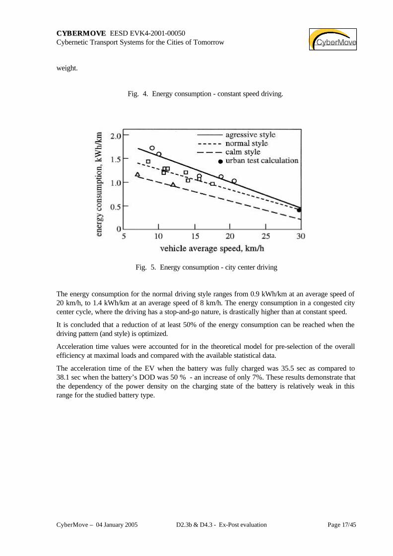
Validation of the model was performed on the example of an electric vehicle (EV) of van type, forwhich detailed experimental data were available. An attempt to obtain an optimization of the weights ofthe main (Zinc-Air) and the auxiliary (Ni-Cd) batteries was undertaken under conditions of theconstant vehicle speed and standard urban drive cycle. Some results are presented in figures 4 and 5.

As an example, a combined weight of the two battery types was taken as 1250 kg, and vehicle weightof 3500 kg. A driving range of 395 km was obtained for the main and auxiliary battery weights of 850and 400 kg, respectively, and an optimal range of 515 km was found for weights of 1100 and 150 kg,respectively. An energy consumption of 0.460 kWh/km and regenerated energy of 0.032 kWh/kmwere obtained for the latter (optimal) case. Different driving styles were also investigated theoreticallyfor the standard urban drive cycle and the same values of the efficiencies, total vehicle and thepropulsion system weights. The above-mentioned results were obtained for the "normal" driving style.A maximal driving range of only 245 km was obtained for the "aggressive" style with an energyconsumption of 0.585 kWh/km and main and auxiliary battery weights of 600 and 650 kg, respectively.Values of the same parameters for "calm" driving style are as follows: range of 755 km, energyconsumption of 0.355 kWh/km, when the propulsion system includes a main battery only, of 1250 kg



weight.

Fig. 4. Energy consumption - constant speed driving.

Fig. 5. Energy consumption - city center driving

The energy consumption for the normal driving style ranges from 0.9 kWh/km at an average speed of20 km/h, to 1.4 kWh/km at an average speed of 8 km/h. The energy consumption in a congested citycenter cycle, where the driving has a stop-and-go nature, is drastically higher than at constant speed.

It is concluded that a reduction of at least 50% of the energy consumption can be reached when thedriving pattern (and style) is optimized.

Acceleration time values were accounted for in the theoretical model for pre-selection of the overallefficiency at maximal loads and compared with the available statistical data.

The acceleration time of the EV when the battery was fully charged was 35.5 sec as compared to38.1 sec when the battery’s DOD was 50 % - an increase of only 7%. These results demonstrate thatthe dependency of the power density on the charging state of the battery is relatively weak in thisrange for the studied battery type.



3. DATA COLLECTION ON CYBERCARS AT SEVERAL SITES

The model presented in the previous Chapter was employed to simulate the behaviour of cybercars infour different sites: INRIA test site, the Technion Campus, the Rivium – 2 loop and the Antibes route.The data collected on vehicles parameters and driving patterns were based on information provided bythe site responsibles and car manufacturers and operators. The main parameters are presented belowfor each of the four sites.

3.1 INRIA TEST SITE

A Yamaha – Europe (YME) vehicle, shown in Fig. 6, was tested in the loop (cycle) at the INRIA testsite. It has been used for demonstrations as well as for tests.

Fig. 6. YME Vehicle at INRIA.

Simulated Vehicle• Gross vehicle weight – 1250 kg• Frontal area – 2.31 m2

• Battery type – Lead-Acid• Maximal DOD – 0.8• Basic battery weight – 126 kg

Simulated Driving Pattern• Driving route – INRIA testing route• Route length – 555 m• Road gradients – as were supplied by INRIA• Driving cycle – as was experimentally measured by INRIA



• Basic average speed – 8.7 km/h

3.2 TECHNION CAMPUS

A CTS was pre-designed for the Technion (Israel Institute of Technology) Campus in Haifa. Thesimulations were performed for the YME vehicle described above, shown in Fig. 6. The route is shownin Fig. 7.

Fig. 7. The CTS route designed for the Technion Campus.

Simulated Vehicle

• Gross vehicle weight – 1250 kg• Frontal area – 2.31 m2

• Battery type – Lead-Acid• Maximal DOD – 0.8• Basic battery weight – 130 kgSimulated Driving Pattern

• Driving route – Technion testing route



• Route length – 1600 m• Absolute averaged value of the road gradients is 7.5%• Driving cycle – as was experimentally measured by TRI• Basic average speed – 12.0 km/h

3.2 RIVIUM - 2 LOOP

Rivium – 2, designed by FROG with their own vehicles (Fig. 8), is scheduled to start operation in thefirst half of 2005. It is an extension of an earlier system, Rivium – 1, which was operated as part of theRotterdam public transportation system. The design figures of the FROG cyber vehicle were used inthe simulations of the Rivium -2 loop.

Fig. 8. FROG vehicle in Rivium - 2

Simulated Vehicle

• Curb vehicle weight (incl. battery) – 4650 kg• Passengers capacity – 20• Frontal area – 5.78 m2

• Battery type – Lead Acid• Maximal road gradient – 5%• Basic battery weight – 1450 kg

Simulated Driving Pattern

• Driving route – RIVIUM 2 site• Total route length – 3.6 km• Maximal road gradient – 5%



• Total number of stops – 10• Basic average speed – 18 km/h

3.3 ANTIBES ROUTE

A cyber car that was used is similar to the one designed and manufactured by FROG for Rivium – 2.It was demonstrated in Antibes in June 2004. on the loop shown in Fig. 9.

Fig. 9. The Antibes CTS route. The circles 1 – 4 represent vehicle crossings, the blue dots pedestriancrossings.

Simulated Vehicle

• Gross vehicle weight – 4650 kg• Passengers capacity – 20• Frontal area – 5.78 m2• Battery type – Pb-Acid• Maximal DOD – 0.8• Basic battery weight – 1450 kg

Simulated Driving Pattern

• Driving route – Antibes testing route• Route length – 2989 m• Plain road• Driving cycle – as experimentally measured in Antibes• Basic average speed – 12.6 km/h



4. ANALYSIS OF DATA ON CYBER CARS

The simulation model was applied using the calculation procedure described below. The whole route ofthe vehicle is divided into N+1 sections (from 0 to N), with the following requirements:

a) The section can include segments of constant drive speed as well as of accelerated / decelerateddrive, but the section is characterized by a single speed value and a single absolute value ofacceleration (deceleration) in each segment.

b) The constant speed value, VC (m/s), is equal to that at the interface between the section of interestand the successive one. In the case of variable speed at the end of the section, a very short segment ofconstant speed is applied.

c) The road gradient and an angle of the travel direction are taken as constant values within the wholesection length.

The section can include several stops, NST, and speed changes, NCH, with the same absolute value ofthe acceleration. 'Stop' is simply full stop of the vehicle , with subsequent return to the constantstationary drive speed for the section, VC, except for the last section (N), where NST = 1 and thefinal speed is equal to 0. 'Speed change' means that VC for the section changes at the sectionacceleration to another value (higher or lower than VC) with an immediate return to VC. In case ofspeed changes in a section, the same pattern was assumed of deceleration and than acceleration (orvice versa) to the constant representative speed.

As noted above, the algorithm can treat two energy sources for the propulsion system, for example amain battery with high energy density and an auxiliary one with high power density. The vehicles in thefour sites had one battery only, so the simulations were performed with a simpler version.

The simulation algorithm and computer code take into account the dependence of the vehicle tractionsystem efficiency on the traction power that depends in turn on the road gradients, the vehicle weight,cross section area, speed and acceleration (deceleration). The dependence of the electrical motorefficiency on the load factor and on the heat losses is taken into account also.

The simulation model was employed for a parametric study, in order to investigate the effects of thebattery weight, the electric motor power and the average speed on the vehicle (or system)performance: driving range, energy consumption and number of passengers moved. For this we definethe vehicle productivity as:

VP = PC*RWhere:PC – passenger capacity of the vehicleR – driving range between battery recharging, km

And number of passengers moved (NPM), for full capacity, as:

NPM = VP / LWhere:



L – route length, km

These definitions apply for a single vehicle on the route as well as for the whole CTS system.

The energy consumption and the driving range (directly related to it) can be calculated for any electricvehicle in any site (on any road or route). The results enable to optimize various parameters, and inparticular the motor maximal power, the vehicle speed and driving pattern and battery weights.Furthermore, it is emphasized that the CTS has an inherent advantage in this respect of energyconservation, since it is operated without drivers, and thus the driving pattern can be programmed in anoptimal manner. The results shown in fig. 5 clearly demonstrate it: the energy consumption stronglydepends on the driver's driving style. Obviously, the CTS performance is independent of humanbehaviour on the road.

In the following results of the simulations are presented for the four sites – INRIA, Technion, Rivium –2 and Antibes, according to the data collected and summarized in Chapter 3. For the Antibes site, astatistical analysis was performed including the total passenger-km travelled: per day, per day in peakhours, per day in off-peak hours; total number of one-way trips, and also for those starting in the above-listed hours; average vehicle occupancy over a day per unit of time and starting in these hours; numberof km - empty vehicles over a day, and the influence of the season on these parameters.

4.1 INRIA TEST SITE

INRIA provided, tin addition to the data in Chapter 3, a map of the site with the corresponding roadgradients and detailed drive parameters: the cyber car speed, distance travelled, etc., as functions oftime, with time-step of 30 ms. Based on these data, the road was partitioned into 34 sections of thesame speed, acceleration and speed change pattern for each of them.

The main simulation results are presented in the figures 10 - 14, for the data on the vehicle, road anddriving pattern of Chapter 3.1. The parametric study is based on the input data.

Fig. 10. Motor power effect on energy consumption.



Fig. 11. Motor power effect on driving range.

Fig. 12. Average speed effect on driving range.



Fig. 13. Effects of battery weight and average speed on vehicle productivity.

Fig. 14. Effects of battery weight and average speed on number of passengers moved.

It is immediately obvious from the results that the vehicle (or system) performance can be optimized:the energy consumption can be minimized, and the driving range can be maximized by selectingappropriate parameters such as battery weight, rated (or maximal) motor power and average vehiclespeed. The latter must be chosen, of course, not only according to the energy considerations but also(and more importantly) to satisfy mobility and safety requirements, for example waiting times.



Figures 10 and 11 show the effects of the rated (or maximal) motor power on the energy consumptionand the related driving range. The appearance of the curves is mainly due to the effects of theefficiencies of the propulsion system components. It can clearly be seen that by careful design andselection of the motor, considerable energy savings can be achieved, with an increase of the drivingrange. This is important also since it leads to better system availability during operation, associated withoptimized system size (number of vehicles). Similarly, the driving pattern, represented here by theaverage velocity, has a strong impact on the energy consumption, as seen in Fig. 12. The effects of thebattery weight and the average speed on the productivity and number of passengers moved areillustrated in Figs. 13 and 14. Again – the maxima of the various curves indicate clearly thatoptimization can be achieved, leading to significant energy savings, increased driving range and bettersystem performance.

4.2 TECHNION CAMPUS

4.2.1 Technion Campus: Statistics Analysis

CTS Project Description

The objective of the CTS project is to improve the accessibility inside the Campus for two mainpopulations:

• Students and visitors arriving by private car who park far from the main buildings.• Public transport riders who have limited mobility inside the Campus, because of the long

walking distances with slopes.

The project is divided into two main phases:

Phase 1: Connection between three big parking lots and some of the faculties in a linear line. Two ofthe parking lots are located close to the Eastern Gate, and the third one is near the main promenade.The line passes near the projected cable car station, which is also located near this gate. This phase isoriented to improve accessibility for students parking far from the main buildings.

The vehicles will have to travel alongside existing traffic. It will be possible to control all theintersections in order to avoid conflicts. The existing right of way comprises two lanes in eachdirection; one of them is generally used for parking, which could be adapted for the CTS vehicles.Therefore, the vehicles can run independently in both directions. At both ends of the line there isenough room to accommodate the vehicles (recharging, storing idle vehicles, etc).

Phase 2: Completion of the initial line to a closed loop that connects most of the faculties and publicbuildings. This phase is oriented to serve both populations listed above. The length of the loop is 2.4 km.

For the purpose of this research, the study was limited to Phase 1 only. Figure 7 shows an aerial photoof the Technion Campus with the proposed line.

Demand Forecast Estimation

To obtain an estimate of the demand for the proposed CTS line, an estimated logit model was used,based on a Stated Preference (SP) study performed in the campus. The statistics analysis for the



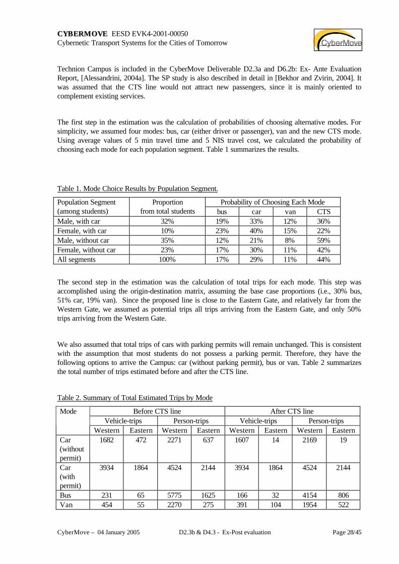
Technion Campus is included in the CyberMove Deliverable D2.3a and D6.2b: Ex- Ante EvaluationReport, [Alessandrini, 2004a]. The SP study is also described in detail in [Bekhor and Zvirin, 2004]. Itwas assumed that the CTS line would not attract new passengers, since it is mainly oriented tocomplement existing services.

The first step in the estimation was the calculation of probabilities of choosing alternative modes. Forsimplicity, we assumed four modes: bus, car (either driver or passenger), van and the new CTS mode.Using average values of 5 min travel time and 5 NIS travel cost, we calculated the probability ofchoosing each mode for each population segment. Table 1 summarizes the results.

Table 1. Mode Choice Results by Population Segment.

Probability of Choosing Each ModePopulation Segment(among students)

Proportionfrom total students bus car van CTS

Male, with car 32% 19% 33% 12% 36%Female, with car 10% 23% 40% 15% 22%Male, without car 35% 12% 21% 8% 59%Female, without car 23% 17% 30% 11% 42%All segments 100% 17% 29% 11% 44%

The second step in the estimation was the calculation of total trips for each mode. This step wasaccomplished using the origin-destination matrix, assuming the base case proportions (i.e., 30% bus,51% car, 19% van). Since the proposed line is close to the Eastern Gate, and relatively far from theWestern Gate, we assumed as potential trips all trips arriving from the Eastern Gate, and only 50%trips arriving from the Western Gate.

We also assumed that total trips of cars with parking permits will remain unchanged. This is consistentwith the assumption that most students do not possess a parking permit. Therefore, they have thefollowing options to arrive the Campus: car (without parking permit), bus or van. Table 2 summarizesthe total number of trips estimated before and after the CTS line.

Table 2. Summary of Total Estimated Trips by Mode

Before CTS line After CTS lineVehicle-trips Person-trips Vehicle-trips Person-trips

Mode

Western Eastern Western Eastern Western Eastern Western EasternCar(withoutpermit)

1682 472 2271 637 1607 14 2169 19

Car(withpermit)

3934 1864 4524 2144 3934 1864 4524 2144

Bus 231 65 5775 1625 166 32 4154 806Van 454 55 2270 275 391 104 1954 522



truck 60 61 60 61 60 61 60 61CTS 0 0 0 0 340 198 2038 1191Total 6361 2517 14900 4742 6497 2274 14900 4742

The results in Table 10 show that a total of 3,229 persons will ride the CTS line in an averageweekday. Assuming an average of 6 persons travelling in each Cybercar, a total of 538 vehicle-tripsare obtained.

The total mode share of the CTS system is 3,229/19,642 = 16%. Since we assumed that the totalnumber of trips will remain unchanged, this means that the CTS system will reduce 720 person-trips bycar, 2440 person-trips by bus and 69 person-trips by shuttle van.

4.2.2 Technion Campus: Energy Consumption Calculations

The Technion Campus data for the vehicle and route are given in Chapter 3. As mentioned above, theCampus is on a rather steep hill and the CTS would be attractive to passengers, who may use it insteadof walking uphill (and downhill too). The average road gradient is 7.5%.

The simulation was performed separately for the two parts of the road – downhill and uphill. Theresults are shown in Fig. 19 and Tables 3 and 4. The effect of battery weight on the cyber carproductivity was investigated and the results are presented in Fig. 19. It is clearly seen, as for theINRIA case presented above, that the curve for the number of passengers moved vs. the batteryweight depicts a maximum, here – at 355 kg (for the specific vehicle, speed and route data). It isdemonstrated, again, that the system can (and should) be designed such as to optimize it.Results for the energy consumption and regeneration for the two road sections (downhill and uphill) andthe whole route, at the average vehicle speed of 12 km/h, are presented in Table 11. It is noted thathere a "hypothetical" vehicle was simulated, with the same shape (frontal area) and same total weightof the vehicle that was used and simulated at the INRIA site, but with various possible passengers'capacity. The results in the Table show that the optimal battery weight is 355 kg. Table 12 includesadditional simulation results with this optimal weight (and 5 passengers in the vehicle). As can be seen,the regenerated energy on the downhill section is very significant. It is therefore emphasized that aregenerative braking system should be included, in order to save energy and to increase the drivingrange. This is an important part of the optimization design of the CTS.



0

50

100

150

200

100 150 200 250 300 350 400 450

battery weight, kg

nu

mb

er o

f p

asse

ng

ers

Fig. 19. Battery weight effect on number of passengers moved.

Table 3. Effects of Battery Weight and Vehicle Passenger Capacity on Energy Consumptionand Regeneration and Driving Range.

Simulation Experiment

1 2 3 4 5

Battery weight (kg) 130 205 280 355 430

Number of passengers ineach car 8 7 6 5 4

Energy consumption perkm (kWh/km) 0.229 0.215 0.218 0.217 0.219

Downward Energyconsumption per km

(kWh/km)0.027 0.028 0.028 0.028 0.028

Upward Energy consumptionper km (kWh/km) 0.465 0.4

14 0.422 0.414 0.418

Regenerated energy per km(kWh/km) 0.052 0.055 0.055 0.055 0.055

Drive range is equal to: (km) 19.2 33.1 44.6 57.1 68.6

Mean speed is: (km/h) 12.0 12.0 12.0 12.0 12.0

Total vehicle-trips for asingle car 12 21 28 36 43

Total person-trips for a singlecar 96 145 167 178 172

Total person-trips needed 3229 3229 3229 3229 3229



Total cars needed to run thesystem 34 22 19 18 19

Total System Consumption(Wh) 147630 158493 188063 43508 94929

Table 4. Energy Consumed and Regenerated

5-Passenger case, battery weight 355 kG

Total energy consumption 124 kWh

Energy consumption per km 0.217 kWh/km

Downward energy consumption 824 Wh


Upward energy consumption 11.5 kWh


Total regenerated energy 3.15 kWh

Regenerated energy per km 0.055 kWh/km

Downward regenerated energy 315 kWh

Regenerated energy per km 0.108 kWh/km

Drive range 57.1 km

Average speed 12 km/h

4.3 RIVIUM - 2 LOOP

The simulation model was employed to investigate the effects of the motor power, the battery weight,the average vehicle speed and the vehicle load (number of passengers) on the driving range and the



vehicle productivity for the RIVIUM - 2 site. Results for the energy consumption are not shown here –they are closely related to the driving range. The results, presented in Figs. 20 – 24, show similartrends as for the INRIA and Technion sites. The driving range decreases with the increase of themotor power (Figs. 20, 21), due to the behaviour of the of the propulsion system efficiency. Obviously,the driving range decrease when the vehicle carries more passengers. The driving range increaseswith average speed (Figs. 22, 23), mainly due to smaller number of accelerations at the higher averagespeeds. This effect is stronger when the route has fewer segments – less stops; the results in Fig. 23represent a case of 10 segments, while those in the other figures here are for 16 segments. It is notedthat at the speed range considered here, the drag forces are not very significant and may have someinfluence only at higher speed values and lower power. In the Antibes site, with a different drivingpattern, a different trend was observed, as discussed below in Chapter 4.4.2.

Fig. 24 shows behaviour of the vehicle productivity under the influence of the battery weight, motorpower and passenger number. It can be seen, similar to the results for the INRIA and Technion sites,that the vehicle productivity increases with up to some “optimal” value, and then starts to decrease.



110

120

130

140

150

160

170

180

190

10 20 30 40 50 60

Motor Power, kw

Dri

vin

g R

ang

e, k

m

Vav=18km/h

Fig. 20. Motor power effect on driving range, 6 passengers, average velocity 18 km/h.

100

110

120

130

140

150

10 20 30 40 50 60

Motor Power, kw

Dri

vin

g R

ang

e, k

m

Vav=14km/h

Fig. 21. Motor power effect on driving range, 20 passengers, average velocity 14 km/h.



110

120

130

140

150

8 9 10 11 12 13 14 15

Average Speed, km/h

Dri

vin

g R

ang

e, k

m

Pmot=35kw

Pmot=22kw

Fig. 22. Effects of average speed and motor power on driving range, 20 passengers.

120

130

140

150

160

170

180

190

8 10 12 14 16 18 20

Average Speed, km/h

Dri

vin

g R

ang

e, k

m

Pmot=18kw

Pmot=22kw

Pmot=35kw

Fig. 23. Effects of average speed and motor power on driving range, 6 passengers.



Fig. 24. Effects of battery weight, motor power and passenger number on vehicle productivity,10 section route, average speed 14km/h.

4.4 ANTIBES ROUTE

4.2.1 Antibes Route: Statistics Analysis

Route

The statistics analysis for the Antibes Route is included in the CyberMove Deliverables D2.3a andD6.2b: Ex-Ante Evaluation Report, [Alessandrini, 2004a], and D2.3b and D4.3: Ex-Post EvaluationReport, [Alessandrini, 2004b]. All the relevant information appears in these reports. The latterreference includes data analysis and simulation results based on the demonstration held in Antibes, inJune 2004, as part of the Project, with the FROG cyber car shown in Fig. 8. Three vehicles were used,with 20 passengers' capacity. These two references include all the relevant information. Somehighlights of the statistics analysis are presented below, taken from the part of the latter Report,prepared and written by TNO.

The track in Antibes, shown in fig. 9, has a total length of 2989 m, that is about 1.5 km from thestation closest to the city center (numbers 6 and 7 in the figure) to the most remote station (numbers 1

2400

2450

2500

2550

2600

2650

2700

2750

2800

2850

2900

1100 1200 1300 1400 1500 1600 1700

Battery Weight, kg

Veh

icle

Pro

du

ctiv

ity,

pas

s

Pmot=35 kw

Pmot=22 kw

20 pas

17pas

25pas



and 12). Compared to the Ex-Ante evaluation, the track is extended with 435 m from stations 3 and 10(parking Vauban) to stations 1 and 12, next to the proposed P+R parking. Also, two more stations havebeen added at this part of the track. The total number of stations (locations on the track where peoplecan get in or out the cyber cars) is 6. The recharging area is located at the end of the track, nearstation 1 and 12. In the recharging area is only space for two cyber cars to charge simultaneously (andnot three, as suggested by the original drawings). At 4 locations on the track, vehicles may cross thetrack to enter or leave a parking or gas station. In total, there are 10 crossing lanes. Pedestrians cancross the road at crosswalks. In total, there are 12 crosswalks for pedestrians, of which 6 near stations.In the simulations, the data of vehicle and pedestrian crossings was considered.

The cyber cars always try to drive with the maximum allowed speed. If they drive slower and there isno obstacle or other cyber car within short, they accelerate with the normal acceleration of the realFROG vehicles - of 0.6 m/s2.

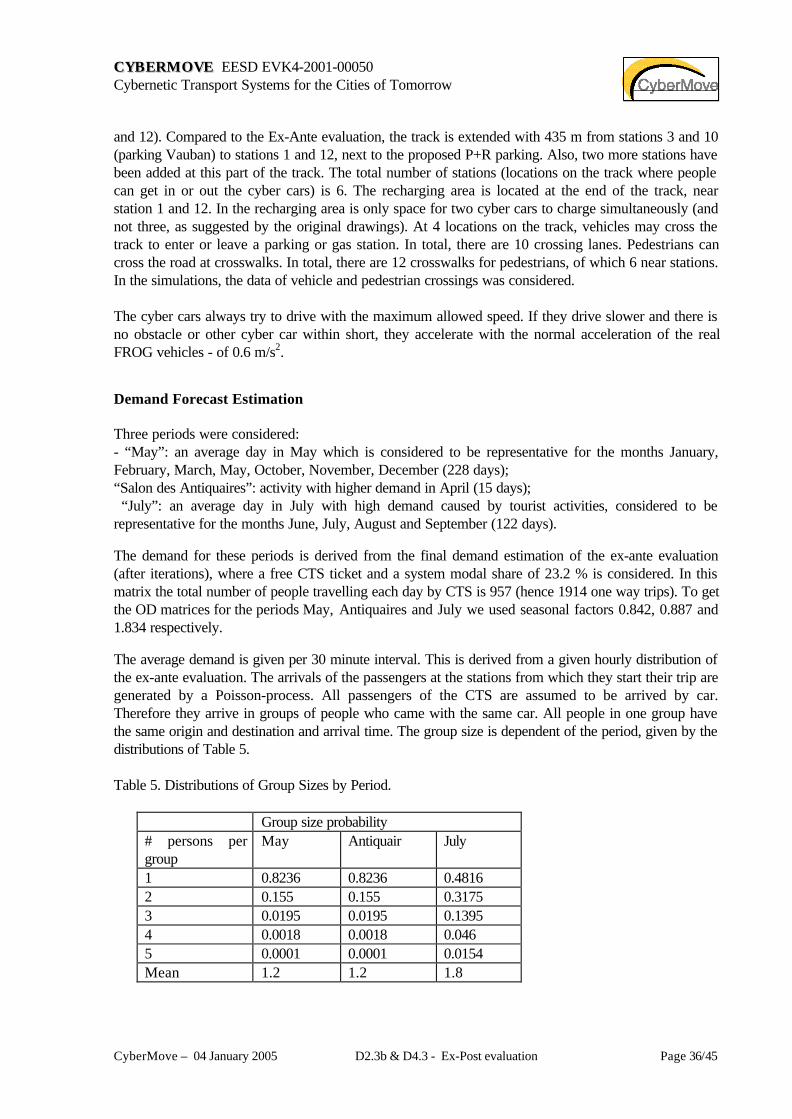
Demand Forecast Estimation

Three periods were considered:- “May”: an average day in May which is considered to be representative for the months January,February, March, May, October, November, December (228 days);“Salon des Antiquaires”: activity with higher demand in April (15 days); “July”: an average day in July with high demand caused by tourist activities, considered to berepresentative for the months June, July, August and September (122 days).

The demand for these periods is derived from the final demand estimation of the ex-ante evaluation(after iterations), where a free CTS ticket and a system modal share of 23.2 % is considered. In thismatrix the total number of people travelling each day by CTS is 957 (hence 1914 one way trips). To getthe OD matrices for the periods May, Antiquaires and July we used seasonal factors 0.842, 0.887 and1.834 respectively.

The average demand is given per 30 minute interval. This is derived from a given hourly distribution ofthe ex-ante evaluation. The arrivals of the passengers at the stations from which they start their trip aregenerated by a Poisson-process. All passengers of the CTS are assumed to be arrived by car.Therefore they arrive in groups of people who came with the same car. All people in one group havethe same origin and destination and arrival time. The group size is dependent of the period, given by thedistributions of Table 5.

Table 5. Distributions of Group Sizes by Period.

Group size probability# persons pergroup

May Antiquair July

1 0.8236 0.8236 0.48162 0.155 0.155 0.31753 0.0195 0.0195 0.13954 0.0018 0.0018 0.0465 0.0001 0.0001 0.0154Mean 1.2 1.2 1.8



Some behaviour components are equal for all members of the same group and some may be differentfor each passenger. Each arriving person pushes a button as soon as he arrives if there are no waitingpeople yet (the button is pushed by only one person for each arriving group). If not all people can boardthe first arriving cyber car, one of the remaining people will push the button again. Passengers will getin and out one by one and passengers will get out before passengers will get in. Passengers board inorder of their waiting times (longest waiting passengers get in first) and they always board if there isstill place in the cyber car (also if groups have to split up). The time for each passenger needed to getin or out the cyber car is normally distributed with mean 2 sec and standard deviation 0.2 sec. This timemay be different for each group member.

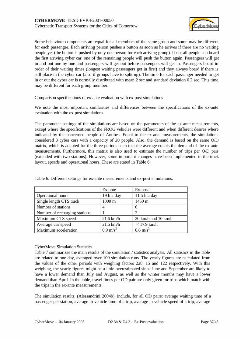
Comparison specifications of ex-ante evaluation with ex-post simulations

We note the most important similarities and differences between the specifications of the ex-anteevaluation with the ex-post simulations.

The parameter settings of the simulations are based on the parameters of the ex-ante measurements,except where the specifications of the FROG vehicles were different and when different desires whereindicated by the concerned people of Antibes. Equal to the ex-ante measurements, the simulationsconsidered 3 cyber cars with a capacity of 20 people. Also, the demand is based on the same O/Dmatrix, which is adapted for the three periods such that the average equals the demand of the ex-antemeasurements. Furthermore, this matrix is also used to estimate the number of trips per O/D pair(extended with two stations). However, some important changes have been implemented in the tracklayout, speeds and operational hours. These are stated in Table 6.

Table 6. Different settings for ex-ante measurements and ex-post simulations.

Ex-ante Ex-postOperational hours 19 h a day 11.5 h a daySingle length CTS track 1000 m 1450 mNumber of stations 4 6Number of recharging stations 1 2Maximum CTS speed 21.6 km/h 20 km/h and 10 km/hAverage car speed 21.6 km/h < 17.9 km/hMaximum acceleration 0.9 m/s2 0.6 m/s2

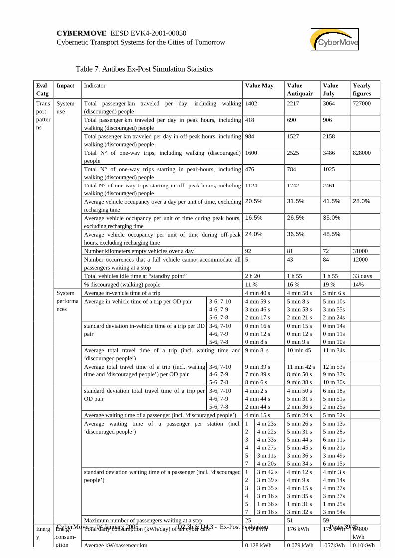
CyberMove Simulation StatisticsTable 7 summarizes the main results of the simulation / statistics analysis. All statistics in the tableare related to one day, averaged over 100 simulation runs. The yearly figures are calculated fromthe values of the other periods with weighing factors 228, 15 and 122 respectively. With thisweighing, the yearly figures might be a little overestimated since June and September are likely tohave a lower demand than July and August, as well as the winter months may have a lowerdemand than April. In the table, travel times per OD pair are only given for trips which match withthe trips in the ex-ante measurements.

The simulation results, (Alessandrini 2004b), include, for all OD pairs: average waiting time of apassenger per station, average in-vehicle time of a trip, average in-vehicle speed of a trip, average



total travel time of a trip (including waiting time), and average speed of a trip (including waitingtime).

One interesting finding from the simulations is that the average speed is rather low. Comparing thiswith normal walking speed, it can be concluded that in this situation, it only rewards in time to goby cyber car from stations 1, 2 and 3 to station 6 at the city center (and back).



Table 7. Antibes Ex-Post Simulation Statistics

EvalCatg

Impact Indicator Value May ValueAntiquair

ValueJuly

Yearlyfigures

Total passenger⋅km traveled per day, including walking(discouraged) people

1402 2217 3064 727000

Total passenger⋅km traveled per day in peak hours, includingwalking (discouraged) people

418 690 906

Total passenger⋅km traveled per day in off-peak hours, includingwalking (discouraged) people

984 1527 2158

Total N° of one-way trips, including walking (discouraged)people

1600 2525 3486 828000

Total N° of one-way trips starting in peak-hours, includingwalking (discouraged) people

476 784 1025

Total N° of one-way trips starting in off- peak-hours, includingwalking (discouraged) people

1124 1742 2461

Average vehicle occupancy over a day per unit of time, excludingrecharging time

20.5% 31.5% 41.5% 28.0%

Average vehicle occupancy per unit of time during peak hours,excluding recharging time

16.5% 26.5% 35.0%

Average vehicle occupancy per unit of time during off-peakhours, excluding recharging time

24.0% 36.5% 48.5%

Number kilometers empty vehicles over a day 92 81 72 31000Number occurrences that a full vehicle cannot accommodate allpassengers waiting at a stop

5 43 84 12000

Total vehicles idle time at “standby point” 2 h 20 1 h 55 1 h 55 33 days

Systemuse

% discouraged (walking) people 11 % 16 % 19 % 14%Average in-vehicle time of a trip 4 min 40 s 4 min 58 s 5 min 6 sAverage in-vehicle time of a trip per OD pair 3-6, 7-10

4-6, 7-95-6, 7-8

4 min 59 s3 min 46 s2 min 17 s


5 mn 10s3 mn 55s2 mn 24s

standard deviation in-vehicle time of a trip per ODpair

3-6, 7-104-6, 7-95-6, 7-8



0 mn 14s0 mn 11s0 mn 10s

Average total travel time of a trip (incl. waiting time and‘discouraged people’)

9 min 8 s 10 min 45 11 m 34s

Average total travel time of a trip (incl. waitingtime and ‘discouraged people’) per OD pair

3-6, 7-104-6, 7-95-6, 7-8


11 min 42 s8 min 50 s9 min 38 s

12 m 53s9 mn 37s10 m 30s

standard deviation total travel time of a trip perOD pair

3-6, 7-104-6, 7-95-6, 7-8



6 mn 18s5 mn 51s2 mn 25s

Average waiting time of a passenger (incl. ‘discouraged people’) 4 min 15 s 5 min 24 s 5 mn 52sAverage waiting time of a passenger per station (incl.‘discouraged people’)

123457

4 m 23s4 m 22s4 m 33s4 m 27s3 m 11s4 m 20s

5 min 26 s5 min 31 s5 min 44 s5 min 45 s3 min 36 s5 min 34 s

5 mn 13s5 mn 28s6 mn 11s6 mn 21s3 mn 49s6 mn 15s

standard deviation waiting time of a passenger (incl. ‘discouragedpeople’)

123457

3 m 42 s3 m 39 s3 m 35 s3 m 16 s1 m 36 s3 m 16 s

4 min 12 s4 min 9 s4 min 15 s3 min 35 s1 min 31 s3 min 32 s

4 min 3 s4 mn 14s4 mn 37s3 mn 37s1 mn 25s3 mn 54s

Transportpatterns

Systemperformances

Maximum number of passengers waiting at a stop 25 51 59Total daily consumption (kWh/day) of all cyber cars 179 kWh 176 kWh 175 kWh 64800

kWhAverage kW/passenger km 0.128 kWh 0.079 kWh .057kWh 0.10kWh

Energy

Energy.consumption



Table 8 presents the main results of the ex-ante and ex-post simulations. A detailed description ofthe results can be found in [Alessandrini, 2004a]. For the purposes of this deliverable, it isnoticeable that the energy consumption is much higher in the ex-ante evaluations. This topic will befurther discussed in the next section.

Table 8. Different results of ex-ante evaluation and ex-post simulations.

Ex-ante Ex-post (average)Modal share 23.2 % 20 %Number of trips 411 2270Vehicle occupancy 11.6 % 28 %Average in-vehicle time of a tripper OD pair

3-64-65-6

3 min2 min1 min


Weighted average in-vehicle timestandard deviation over trips 3-6, 4-6and 5-6

4.3 s 11.8 s

Average waiting time 1 min 15 s 4 min 50 sWeighted average waiting time standarddeviation

7 s 3 min 27 s

Daily energy consumption 971 kWh 178 kWhAverage kWh/p*km 0.51 kWh/ p*km 0.1 kWh/ p*km

p*km = passenger * km

4.2.2 Antibes Route : Energy Consumption Calculations

Energy consumption calculations have been preformed by three partners of the Project Consortium:TNO, DITS and TRI, by using their own simulation models. They have investigated several aspects ofthe energy consumption issues. The TNO model is described in the CyberMove Deliverable D2.3b andD4.3: Ex-Post Evaluation Report, [Alessandrini, 2004b]. The DITS model is described in theCyberCars Deliverable D3: New Technologies for Infrastructures, [Immens, 2003]. The TRI model isdescribed in Chapter 2 above. It is noted that the latter is based on simulation of the behaviour of asingle vehicle, while the former two simulate not only the CTS energy consumption, but the entiresystem functioning. The main results of these studies are presented and summarized here.

The TNO and DITS model were employed in the CyberCars and CyberMove Projects mainly for sitesimulations, and in particular the Antibes Route, where actual operation of CTS's was carried outduring the demonstrations in June 2004, within the framework of the Projects. The TRI model wasemployed here mainly for parametric studies, in order to identify ways to optimize CTS energyconsumption and driving range.

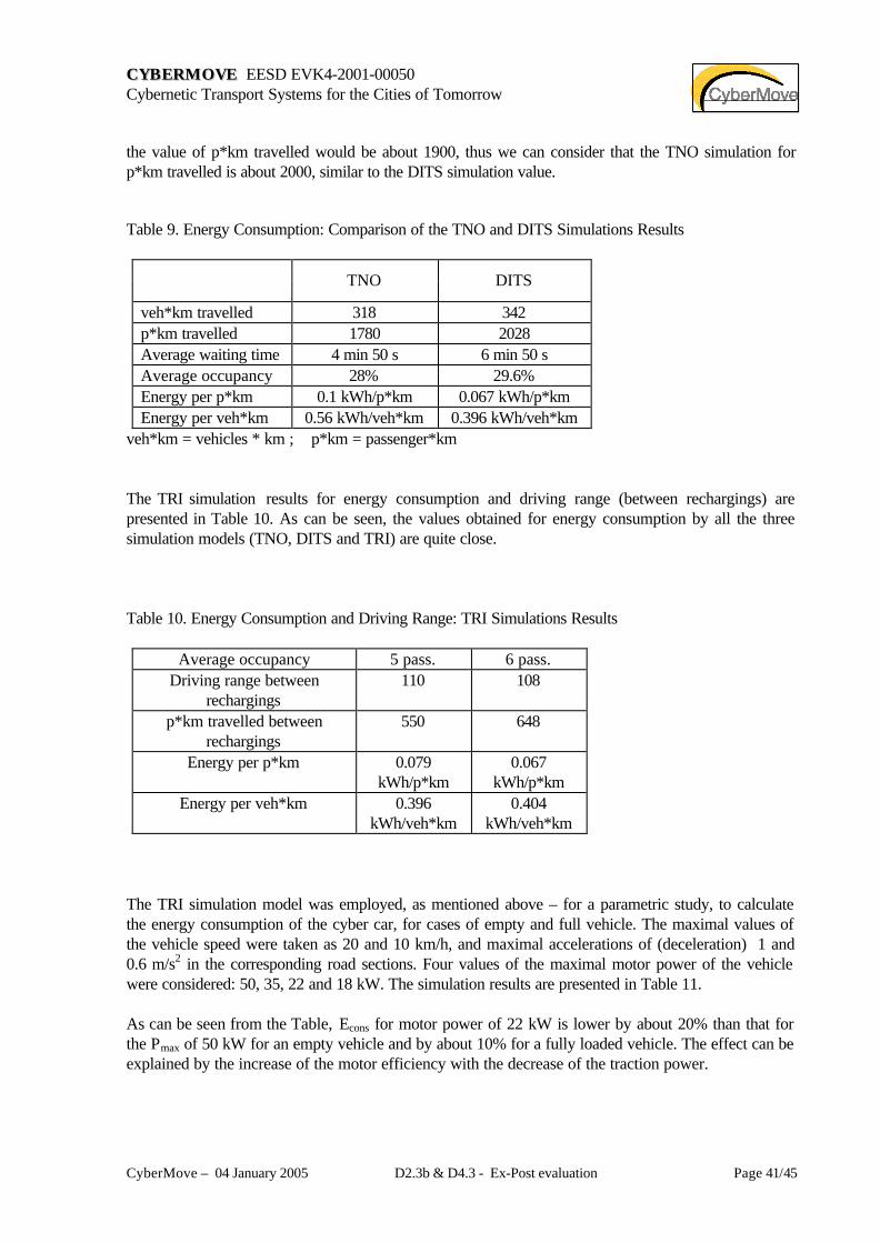
A comparison of the TNO and DITS results is presented in Table 9. The differences between thenumbers of p*km travelled are mainly due to different approximations: in the TNO simulations, the totalenergy consumption is 178 kWh and that for per p*km is 0.1 kWh/p*km, thus the total number of dailyp*km travelled is 178/0.1 = 1780. If the value of 0.1 kWh/p*km would have been lower, the number ofp*km would be larger. For example, if the energy consumed per p*km was precisely 0.095 kWh/p*km,



the value of p*km travelled would be about 1900, thus we can consider that the TNO simulation forp*km travelled is about 2000, similar to the DITS simulation value.

Table 9. Energy Consumption: Comparison of the TNO and DITS Simulations Results

TNO DITS

veh*km travelled 318 342p*km travelled 1780 2028Average waiting time 4 min 50 s 6 min 50 sAverage occupancy 28% 29.6%Energy per p*km 0.1 kWh/p*km 0.067 kWh/p*kmEnergy per veh*km 0.56 kWh/veh*km 0.396 kWh/veh*km

veh*km = vehicles * km ; p*km = passenger*km

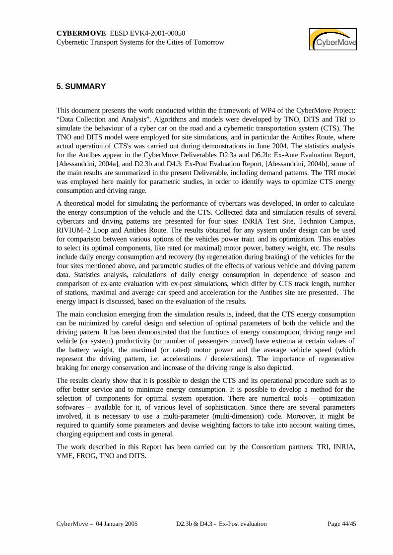
The TRI simulation results for energy consumption and driving range (between rechargings) arepresented in Table 10. As can be seen, the values obtained for energy consumption by all the threesimulation models (TNO, DITS and TRI) are quite close.

Table 10. Energy Consumption and Driving Range: TRI Simulations Results

Average occupancy 5 pass. 6 pass.Driving range between

rechargings110 108

p*km travelled betweenrechargings

550 648

Energy per p*km 0.079kWh/p*km

0.067kWh/p*km

Energy per veh*km 0.396kWh/veh*km

0.404kWh/veh*km

The TRI simulation model was employed, as mentioned above – for a parametric study, to calculatethe energy consumption of the cyber car, for cases of empty and full vehicle. The maximal values ofthe vehicle speed were taken as 20 and 10 km/h, and maximal accelerations of (deceleration) 1 and0.6 m/s2 in the corresponding road sections. Four values of the maximal motor power of the vehiclewere considered: 50, 35, 22 and 18 kW. The simulation results are presented in Table 11.

As can be seen from the Table, Econs for motor power of 22 kW is lower by about 20% than that forthe Pmax of 50 kW for an empty vehicle and by about 10% for a fully loaded vehicle. The effect can beexplained by the increase of the motor efficiency with the decrease of the traction power.



It is noted that there are no energy consumption and driving range values listed in Table 11 for the lowmotor power - 18 kW, and vehicle with full capacity. The reason for this is the lack of enough powerto propel the vehicle at the maximal stipulated acceleration in the case.

Table 11. Energy Consumption: TRI Simulation Results.

Energy Consumption per km,kWh/km Driving Range, km

Pmax, kWEmpty Full Load Empty Full Load

50 0.460 0.563 91 75

35 0.406 0.511 105 84

22 0.364 0.509 119 86

18 0.362 --------- 120 ----------

It is emphasized, again, that the motor power can be optimized, based on pre-designed acceleration andspeed values, i.e. desired driving pattern.

Fig. 25 shows the effects of the battery weight and the average speed on the vehicle productivity(number of passengers moved). It is observed, again, that there is a maximum for certain values ofthese parameters, so it is possible to design the system for optimized energy consumption.

It is interesting to note that unlike the behaviour of the curves for the Rivium – 2 case (Chapter 4.3).Here, for the Antibes case, the vehicle productivity decreases with the increases of the average speed.This is due to the rather large number of stops and of pedestrian crossings, so that there are manyspeed changes and accelerations that require more energy.



620

640

660

680

700

720

740

760

780

1100 1300 1500 1700

battery weight

nu

mb

er o

f pas

sen

ger

s

v=12.1km/h

v=10.3km/h

Fig. 25. Effects of battery weight and average speed on number of passengers moved.



5. SUMMARY

This document presents the work conducted within the framework of WP4 of the CyberMove Project:“Data Collection and Analysis”. Algorithms and models were developed by TNO, DITS and TRI tosimulate the behaviour of a cyber car on the road and a cybernetic transportation system (CTS). TheTNO and DITS model were employed for site simulations, and in particular the Antibes Route, whereactual operation of CTS's was carried out during demonstrations in June 2004. The statistics analysisfor the Antibes appear in the CyberMove Deliverables D2.3a and D6.2b: Ex-Ante Evaluation Report,[Alessandrini, 2004a], and D2.3b and D4.3: Ex-Post Evaluation Report, [Alessandrini, 2004b], some ofthe main results are summarized in the present Deliverable, including demand patterns. The TRI modelwas employed here mainly for parametric studies, in order to identify ways to optimize CTS energyconsumption and driving range.

A theoretical model for simulating the performance of cybercars was developed, in order to calculatethe energy consumption of the vehicle and the CTS. Collected data and simulation results of severalcybercars and driving patterns are presented for four sites: INRIA Test Site, Technion Campus,RIVIUM–2 Loop and Antibes Route. The results obtained for any system under design can be usedfor comparison between various options of the vehicles power train and its optimization. This enablesto select its optimal components, like rated (or maximal) motor power, battery weight, etc. The resultsinclude daily energy consumption and recovery (by regeneration during braking) of the vehicles for thefour sites mentioned above, and parametric studies of the effects of various vehicle and driving patterndata. Statistics analysis, calculations of daily energy consumption in dependence of season andcomparison of ex-ante evaluation with ex-post simulations, which differ by CTS track length, numberof stations, maximal and average car speed and acceleration for the Antibes site are presented. Theenergy impact is discussed, based on the evaluation of the results.

The main conclusion emerging from the simulation results is, indeed, that the CTS energy consumptioncan be minimized by careful design and selection of optimal parameters of both the vehicle and thedriving pattern. It has been demonstrated that the functions of energy consumption, driving range andvehicle (or system) productivity (or number of passengers moved) have extrema at certain values ofthe battery weight, the maximal (or rated) motor power and the average vehicle speed (whichrepresent the driving pattern, i.e. accelerations / decelerations). The importance of regenerativebraking for energy conservation and increase of the driving range is also depicted.

The results clearly show that it is possible to design the CTS and its operational procedure such as tooffer better service and to minimize energy consumption. It is possible to develop a method for theselection of components for optimal system operation. There are numerical tools – optimizationsoftwares – available for it, of various level of sophistication. Since there are several parametersinvolved, it is necessary to use a multi-parameter (multi-dimension) code. Moreover, it might berequired to quantify some parameters and devise weighting factors to take into account waiting times,charging equipment and costs in general.

The work described in this Report has been carried out by the Consortium partners: TRI, INRIA,YME, FROG, TNO and DITS.



REFERENCES

Alessandrini, A. 2004a. Ex- Ante Evaluation Report. CyberMove Deliverable D2.3a and D6.2b.

Alessandrini, A. 2004b. Ex- Post Evaluation Report. CyberMove Deliverable D2.3b and D4.3.

Bekhor, S. and Zvirin, Y, 2004. Estimating the Potential Use of Cybernetic Cars for a UniversityCampus. Paper presented at the 10th World Conference in Transport Research, Istanbul, Turkey.

Bosch, G. 1996. Automotive Handbook, 4-th edition, SAE Society of Automotive Engineers,Warrendale, PA USA.

Caraceni, A. Cipolla, G. & Barbiero, R. 1998. Hybrid Power Unit Development for Fiat MultiplaVehicle, 981124, Society of Automotive Engineers.

Ehsani, M., Yimin, G. & Buttler, L. 1999K. Design Optimization of Electrically Peaking HybridVehicles, Texas A&M University, Advanced Vehicles System Research Program, College Station, TX77843-3128.

Harats, Y., Koretz, Y., Goldstein, B. J. & Korall, M. 1995. The Electric Fuel System Solution forElectric Vehicles. Presented at “Batteries und Batteriemanagement” Conf. Essen, Germany.

Hochgraf, C. G., Ryan, M. J. & Wiegman, H. L. 1996. Engine Control strategy for a series HybridElectric Vehicle Incorporating Load Levelling and Computer Controlled Energy Management, SAE960230.

Immens A. 2003. New Technologies for Infrastructures. CyberCars Deliverable D3.

Kottick, D., Tartakovsky, L. Gutman, M. & Zvirin Y. 2000. Results of electric vehicle demonstrationprogram. Proceedings IEEE Conference, Tel-Aviv, 318 – 321.

Meier-Engel, K. 2000. Failure Time and Energy Consumption of Vehicles. Matador Contract ReportJOE3-CT97-0081.

Nicol, B. D. & Rand, D. A. J. 1984. Power Sources for Electric Vehicles, Elsevier.

SIMPLEV, 2000. SIMPLEV, Simulating Electric&Hybrid Vehicles, http://ev.inel.gov/simplev/pg2.html

DATA COLLECTION AND ANALYSIS - Technion

Documents

Transcript of DATA COLLECTION AND ANALYSIS - Technion