1

Paper 1603-2014

Data Coarsening and Data Swapping Algorithms

Tom Krenzke, Katie Hubbell, Mamadou Diallo,

Amita Gopinath, Sixia Chen

Westat, 1600 Research Blvd, Rockville MD, 20850

ABSTRACT

With increased concern about privacy and, at the same time, pressure to make survey data available,

statistical disclosure control (SDC) treatments are performed on survey microdata to reduce disclosure

risk prior to dissemination to the public. Making the time to conduct the necessary SDC treatments is all

the more problematic in the push to provide data online for immediate user query. Two SDC

approaches are data coarsening, which reduces the information collected, and data swapping, which is

used to adjust data values. Data coarsening includes recodes, top/bottom codes, and variable

suppression. Challenges related to creating a SAS® macro for data coarsening include providing flexibility

for conducting different coarsening approaches and keeping track of the changes to the data so that

variable and value labels can be assigned correctly. Data swapping includes selecting target records for

swapping, finding swapping partners, and swapping data values for the target variables. With the goal of

minimizing the impact on resulting estimates, challenges for data swapping are to find swapping

partners that are close matches in terms of both unordered categorical and ordered categorical

variables, to ensure that enough change is made to the target variables, to retain data consistency

among variables, and to control the pool of potential swapping partners. An example is presented using

each algorithm.

INTRODUCTION

There has been increased pressure to provide microdata to the general public online for immediate use

in less time. However, because of disclosure concerns, time is needed to review the dataset very closely

and cautiously, since combinations of indirect identifiers can reveal the identities of individuals. Time is

also needed to apply confidentiality edits that help to reduce the risk of data disclosure. The purpose of

treating the underlying microdata is to add uncertainty to the identification of a sampled individual in

the dataset. We refer to the process as statistical disclosure control (SDC). Standardization helps to

reduce program development costs, ensures that the same approved process is used consistently

throughout the organization, makes it easier to review the processing results, and reduces the overall

time to accomplish the task.

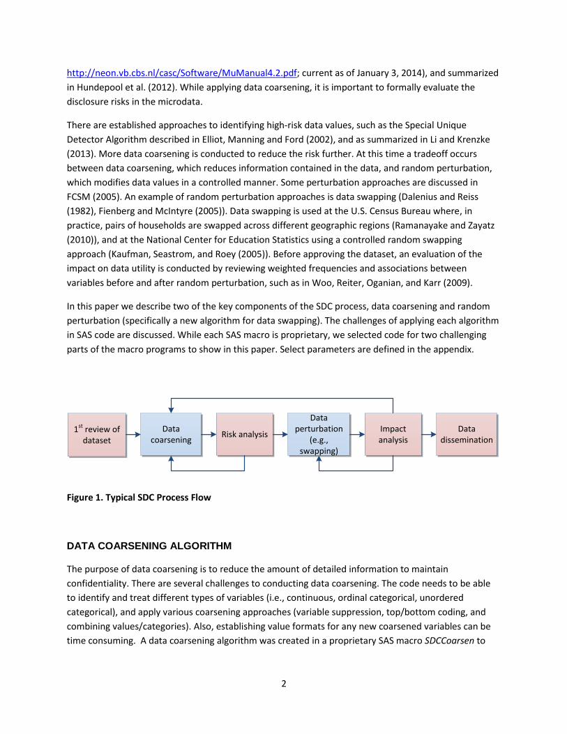
Figure 1 illustrates a typical SDC process flow. It begins with a first review of the microdata file to get

familiar with the set of variables, their types, number of categories, missing value codes, and structural

reporting patterns. Then an initial data coarsening step is taken, which may include recoding,

top/bottom-coding (trimming high/low outlier values to a cutoff), and variable suppression. A discussion

of data coarsening can be found in the mu-Argus 4.2 manual (available at

2

http://neon.vb.cbs.nl/casc/Software/MuManual4.2.pdf; current as of January 3, 2014), and summarized

in Hundepool et al. (2012). While applying data coarsening, it is important to formally evaluate the

disclosure risks in the microdata.

There are established approaches to identifying high-risk data values, such as the Special Unique

Detector Algorithm described in Elliot, Manning and Ford (2002), and as summarized in Li and Krenzke

(2013). More data coarsening is conducted to reduce the risk further. At this time a tradeoff occurs

between data coarsening, which reduces information contained in the data, and random perturbation,

which modifies data values in a controlled manner. Some perturbation approaches are discussed in

FCSM (2005). An example of random perturbation approaches is data swapping (Dalenius and Reiss

(1982), Fienberg and McIntyre (2005)). Data swapping is used at the U.S. Census Bureau where, in

practice, pairs of households are swapped across different geographic regions (Ramanayake and Zayatz

(2010)), and at the National Center for Education Statistics using a controlled random swapping

approach (Kaufman, Seastrom, and Roey (2005)). Before approving the dataset, an evaluation of the

impact on data utility is conducted by reviewing weighted frequencies and associations between

variables before and after random perturbation, such as in Woo, Reiter, Oganian, and Karr (2009).

In this paper we describe two of the key components of the SDC process, data coarsening and random

perturbation (specifically a new algorithm for data swapping). The challenges of applying each algorithm

in SAS code are discussed. While each SAS macro is proprietary, we selected code for two challenging

parts of the macro programs to show in this paper. Select parameters are defined in the appendix.

1st review of dataset

Data coarsening

Risk analysis

Data perturbation

(e.g., swapping)

Impact analysis

Data dissemination

Figure 1. Typical SDC Process Flow

DATA COARSENING ALGORITHM

The purpose of data coarsening is to reduce the amount of detailed information to maintain

confidentiality. There are several challenges to conducting data coarsening. The code needs to be able

to identify and treat different types of variables (i.e., continuous, ordinal categorical, unordered

categorical), and apply various coarsening approaches (variable suppression, top/bottom coding, and

combining values/categories). Also, establishing value formats for any new coarsened variables can be

time consuming. A data coarsening algorithm was created in a proprietary SAS macro SDCCoarsen to

3

conduct the following data coarsening approaches: variable suppression, combining values of

continuous or ordinal variables, and grouping levels of categorical variables. Each is described further in

the following paragraphs.

Variable suppression allows the data producer to remove from the dataset any variables that can reveal

the identity of a participant to the survey. The obvious variables to remove are the personally

identifiable information (PII) such as name, date of birth, addresses, specific date of events, etc. Non-PII

variables can also be suppressed if they can reveal identity of a respondent when crossed with other

variables. The best candidates for variable suppression are binary factual variables with few responses

to one of the levels, which therefore identifies a rare event.

Combining values of continuous or ordinal variables occurs in three ways in the macro: top/bottom

coding, records with arbitrary subgroups, and recodes with percentile cutoffs. Top/bottom coding

modifies the distribution of the variable by shrinking the tails. The data user can decide to top code,

bottom code, or do both. Top coding consists of trimming a variable to some maximum value. For

instance, age can be top coded to 85 years old which means all aged 85 or older are given age 85 and all

younger than 85 keep their age on the public use file. Similarly, bottom coding consists of setting smaller

values than a threshold to a specified minimum value. In addition, SDCCoarsen has two ways of doing

recodes. The first way is by using specified cutoff points to create the intervals. For instance, a variable

containing single years of age can be categorized in age groups (0-15, 16-24, 25-34, 45-54, 55-64, 65+).

The second way uses the percentile of the distribution of the variable to create a specified number of

intervals. For instance, the quartiles can be used to create four intervals.

Recoding categorical variables consists of merging levels of a variable to form broader categories. The

idea is to combine levels with small frequencies so that the resulting recoded variable will have more

units in the combined cells. The macro creates new coarsened variables and value formats (if provided

by the user).

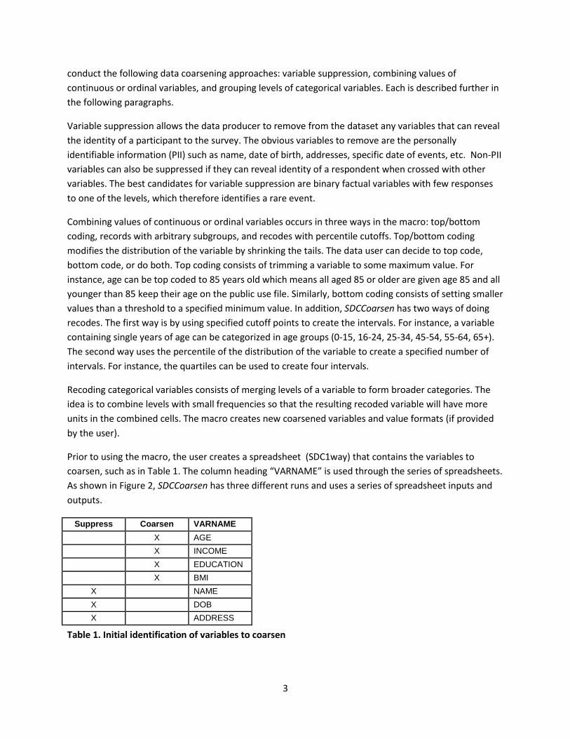
Prior to using the macro, the user creates a spreadsheet (SDC1way) that contains the variables to

coarsen, such as in Table 1. The column heading “VARNAME” is used through the series of spreadsheets.

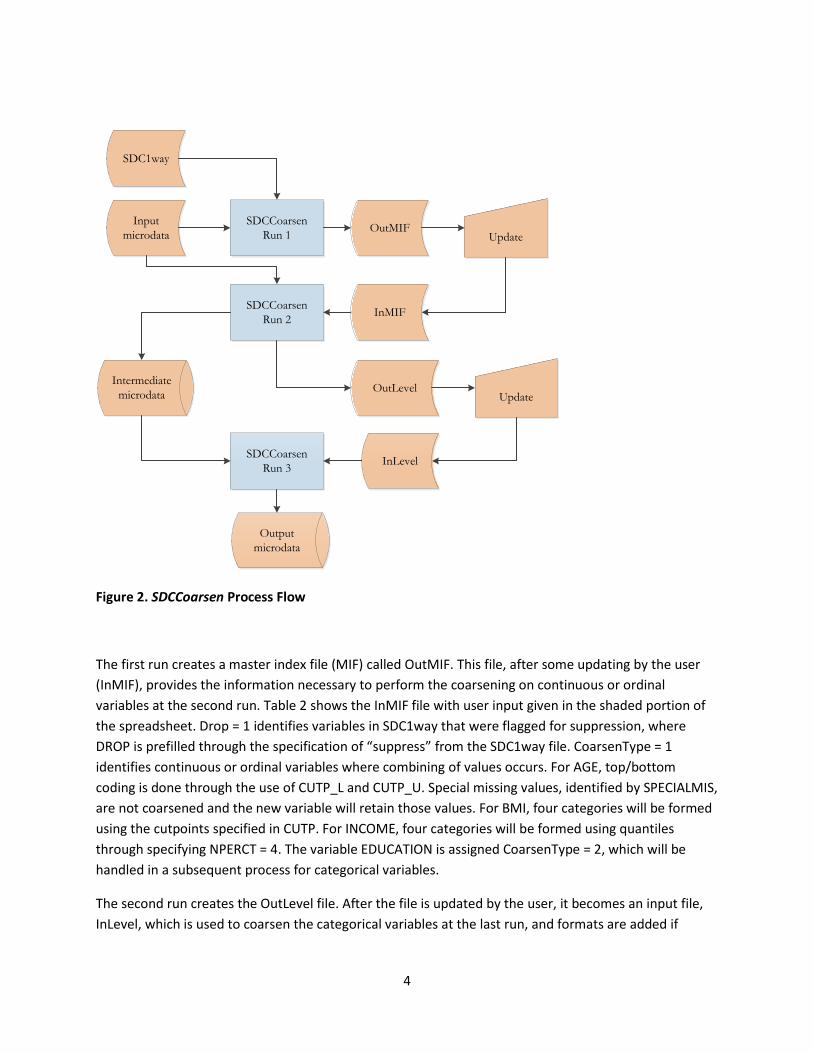
As shown in Figure 2, SDCCoarsen has three different runs and uses a series of spreadsheet inputs and

outputs.

Suppress Coarsen VARNAME

X AGE

X INCOME

X EDUCATION

X BMI

X NAME

X DOB

X ADDRESS

Table 1. Initial identification of variables to coarsen

4

SDCCoarsen

Run 2

SDCCoarsen

Run 1OutMIF

Intermediate

microdata

Update

InMIF

SDCCoarsen

Run 3

OutLevelUpdate

InLevel

Output

microdata

SDC1way

Input

microdata

Figure 2. SDCCoarsen Process Flow

The first run creates a master index file (MIF) called OutMIF. This file, after some updating by the user

(InMIF), provides the information necessary to perform the coarsening on continuous or ordinal

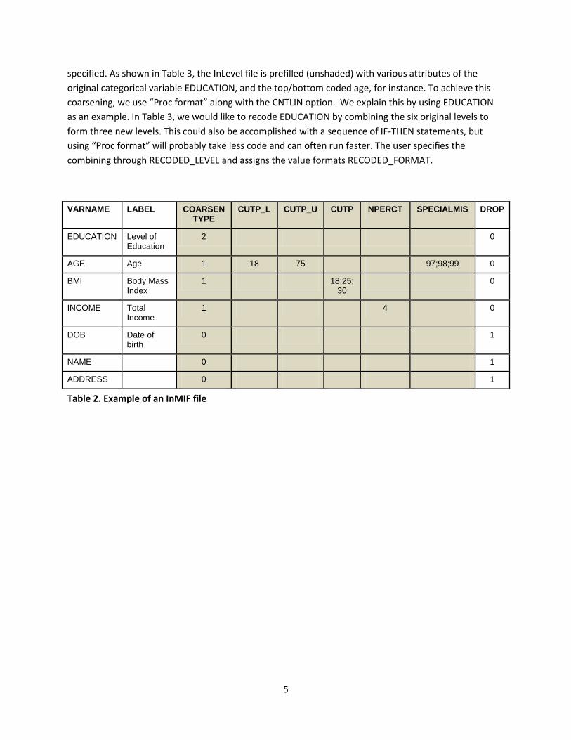
variables at the second run. Table 2 shows the InMIF file with user input given in the shaded portion of

the spreadsheet. Drop = 1 identifies variables in SDC1way that were flagged for suppression, where

DROP is prefilled through the specification of “suppress” from the SDC1way file. CoarsenType = 1

identifies continuous or ordinal variables where combining of values occurs. For AGE, top/bottom

coding is done through the use of CUTP_L and CUTP_U. Special missing values, identified by SPECIALMIS,

are not coarsened and the new variable will retain those values. For BMI, four categories will be formed

using the cutpoints specified in CUTP. For INCOME, four categories will be formed using quantiles

through specifying NPERCT = 4. The variable EDUCATION is assigned CoarsenType = 2, which will be

handled in a subsequent process for categorical variables.

The second run creates the OutLevel file. After the file is updated by the user, it becomes an input file,

InLevel, which is used to coarsen the categorical variables at the last run, and formats are added if

5

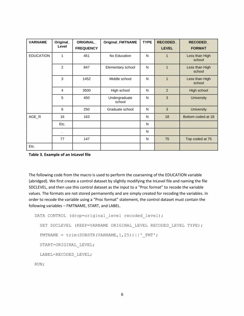
specified. As shown in Table 3, the InLevel file is prefilled (unshaded) with various attributes of the

original categorical variable EDUCATION, and the top/bottom coded age, for instance. To achieve this

coarsening, we use “Proc format” along with the CNTLIN option. We explain this by using EDUCATION

as an example. In Table 3, we would like to recode EDUCATION by combining the six original levels to

form three new levels. This could also be accomplished with a sequence of IF-THEN statements, but

using “Proc format” will probably take less code and can often run faster. The user specifies the

combining through RECODED_LEVEL and assigns the value formats RECODED_FORMAT.

VARNAME LABEL COARSENTYPE

CUTP_L CUTP_U CUTP NPERCT SPECIALMIS DROP

EDUCATION Level of Education

2 0

AGE Age 1 18 75 97;98;99 0

BMI Body Mass Index

1 18;25;30

0

INCOME Total Income

1 4 0

DOB Date of birth

0 1

NAME 0 1

ADDRESS 0 1

Table 2. Example of an InMIF file

6

VARNAME Original_Level

ORIGINAL_

FREQUENCY

Original_FMTNAME TYPE RECODED_

LEVEL

RECODED_

FORMAT

EDUCATION

1 451 No Education N 1 Less than High school

2 847 Elementary school N 1 Less than High school

3 1452 Middle school N 1 Less than High school

4 3500 High school N 2 High school

5 450 Undergraduate school

N 3 University

6 250 Graduate school N 3 University

AGE_R 16 163 N 18 Bottom coded at 18

Etc. N

. N

77 147 N 75 Top coded at 75

Etc.

Table 3. Example of an InLevel file

The following code from the macro is used to perform the coarsening of the EDUCATION variable

(abridged). We first create a control dataset by slightly modifying the InLevel file and naming the file

SDCLEVEL, and then use this control dataset as the input to a “Proc format” to recode the variable

values. The formats are not stored permanently and are simply created for recoding the variables. In

order to recode the variable using a “Proc format” statement, the control dataset must contain the

following variables – FMTNAME, START, and LABEL.

DATA CONTROL (drop=original_level recoded_level);

SET SDCLEVEL (KEEP=VARNAME ORIGINAL_LEVEL RECODED_LEVEL TYPE);

FMTNAME = trim(SUBSTR(VARNAME,1,25))||'_FMT';

START=ORIGINAL_LEVEL;

LABEL=RECODED_LEVEL;

RUN;

7

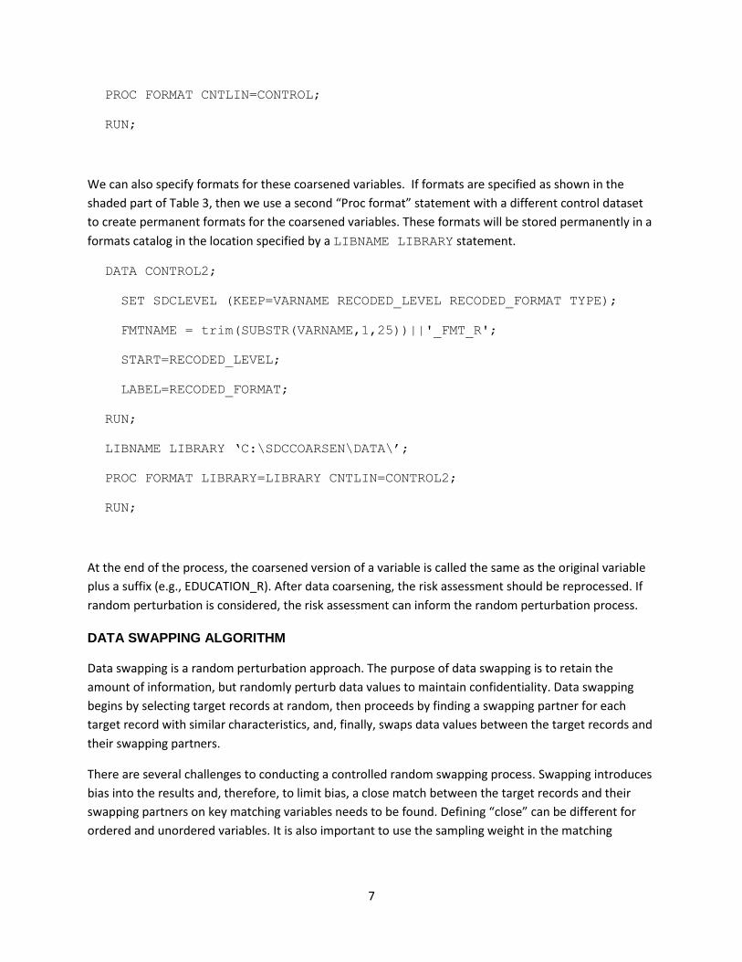
PROC FORMAT CNTLIN=CONTROL;

RUN;

We can also specify formats for these coarsened variables. If formats are specified as shown in the

shaded part of Table 3, then we use a second “Proc format” statement with a different control dataset

to create permanent formats for the coarsened variables. These formats will be stored permanently in a

formats catalog in the location specified by a LIBNAME LIBRARY statement.

DATA CONTROL2;

SET SDCLEVEL (KEEP=VARNAME RECODED_LEVEL RECODED_FORMAT TYPE);

FMTNAME = trim(SUBSTR(VARNAME,1,25))||'_FMT_R';

START=RECODED_LEVEL;

LABEL=RECODED_FORMAT;

RUN;

LIBNAME LIBRARY ‘C:\SDCCOARSEN\DATA\’;

PROC FORMAT LIBRARY=LIBRARY CNTLIN=CONTROL2;

RUN;

At the end of the process, the coarsened version of a variable is called the same as the original variable

plus a suffix (e.g., EDUCATION_R). After data coarsening, the risk assessment should be reprocessed. If

random perturbation is considered, the risk assessment can inform the random perturbation process.

DATA SWAPPING ALGORITHM

Data swapping is a random perturbation approach. The purpose of data swapping is to retain the

amount of information, but randomly perturb data values to maintain confidentiality. Data swapping

begins by selecting target records at random, then proceeds by finding a swapping partner for each

target record with similar characteristics, and, finally, swaps data values between the target records and

their swapping partners.

There are several challenges to conducting a controlled random swapping process. Swapping introduces

bias into the results and, therefore, to limit bias, a close match between the target records and their

swapping partners on key matching variables needs to be found. Defining “close” can be different for

ordered and unordered variables. It is also important to use the sampling weight in the matching

8

process, since this weight is used in all estimates generated from the data records. A mechanical

challenge is to control the pool of potential swapping partners as partners are identified. Also, handling

structural response patterns (e.g., skip patterns), and retaining consistency among variables (such as

different versions of race variables) should be among the goals of swapping.

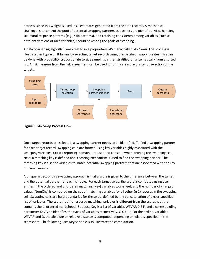
A data coarsening algorithm was created in a proprietary SAS macro called SDCSwap. The process is

illustrated in Figure 3. It begins by selecting target records using prespecified swapping rates. This can

be done with probability proportionate to size sampling, either stratified or systematically from a sorted

list. A risk measure from the risk assessment can be used to form a measure of size for selection of the

targets.

Swapping partner selection

Target swap selection

Input microdata

SwapOutput

microdata

OrderedScoresheet

UnorderedScoresheet

Swapping rates

Figure 3. SDCSwap Process Flow

Once target records are selected, a swapping partner needs to be identified. To find a swapping partner

for each target record, swapping cells are formed using key variables highly associated with the

swapping variables. Critical reporting domains are useful to consider when defining the swapping cell.

Next, a matching key is defined and a scoring mechanism is used to find the swapping partner. The

matching key is a set of variables to match potential swapping partners that are associated with the key

outcome variables.

A unique aspect of this swapping approach is that a score is given to the difference between the target

and the potential partner for each variable. For each target swap, the score is computed using user

entries in the ordered and unordered matching (Key) variables worksheet, and the number of changed

values (NumChg) is computed on the set of matching variables for all other (n-1) records in the swapping

cell. Swapping cells are hard boundaries for the swap, defined by the concatenation of a user-specified

list of variables. The scoresheet for ordered matching variables is different from the scoresheet that

contains the unordered scoresheets. Suppose Key is a list of variables WTVAR D E F, and a corresponding

parameter KeyType identifies the types of variables respectively, O O U U. For the ordinal variables

WTVAR and D, the absolute or relative distance is computed, depending on what is specified in the

scoresheet. The following uses Key variable D to illustrate the computation.

9

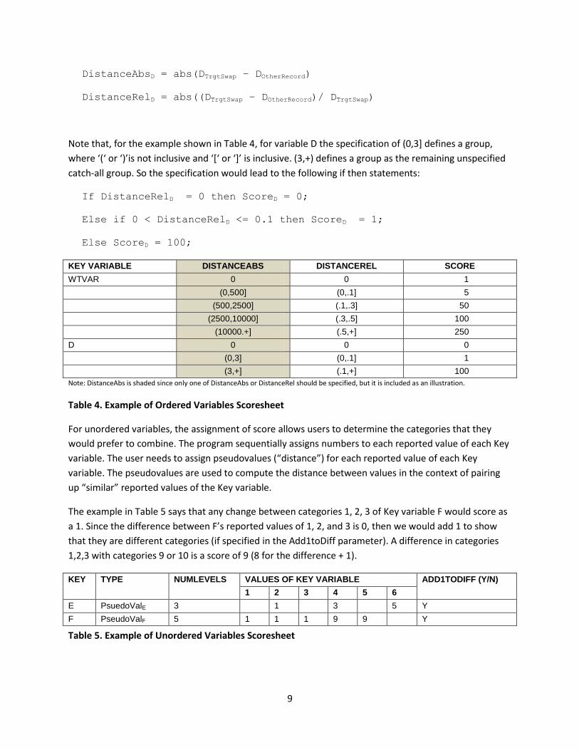
DistanceAbsD = abs(DTrgtSwap – DOtherRecord)

DistanceRelD = abs((DTrgtSwap – DOtherRecord)/ DTrgtSwap)

Note that, for the example shown in Table 4, for variable D the specification of (0,3] defines a group,

where ‘(‘ or ‘)’is not inclusive and ‘[‘ or ‘]’ is inclusive. (3,+) defines a group as the remaining unspecified

catch-all group. So the specification would lead to the following if then statements:

If DistanceRelD = 0 then ScoreD = 0;

Else if 0 < DistanceRelD <= 0.1 then ScoreD = 1;

Else ScoreD = 100;

KEY VARIABLE DISTANCEABS DISTANCEREL SCORE

WTVAR 0 0 1

(0,500] (0,.1] 5

(500,2500] (.1,.3] 50

(2500,10000] (.3,.5] 100

(10000.+] (.5,+] 250

D 0 0 0

(0,3] (0,.1] 1

(3,+] (.1,+] 100

Note: DistanceAbs is shaded since only one of DistanceAbs or DistanceRel should be specified, but it is included as an illustration.

Table 4. Example of Ordered Variables Scoresheet

For unordered variables, the assignment of score allows users to determine the categories that they

would prefer to combine. The program sequentially assigns numbers to each reported value of each Key

variable. The user needs to assign pseudovalues (“distance”) for each reported value of each Key

variable. The pseudovalues are used to compute the distance between values in the context of pairing

up “similar” reported values of the Key variable.

The example in Table 5 says that any change between categories 1, 2, 3 of Key variable F would score as

a 1. Since the difference between F’s reported values of 1, 2, and 3 is 0, then we would add 1 to show

that they are different categories (if specified in the Add1toDiff parameter). A difference in categories

1,2,3 with categories 9 or 10 is a score of 9 (8 for the difference + 1).

KEY TYPE NUMLEVELS VALUES OF KEY VARIABLE ADD1TODIFF (Y/N)

1 2 3 4 5 6

E PsuedoValE 3 1 3 5 Y

F PseudoValF 5 1 1 1 9 9 Y

Table 5. Example of Unordered Variables Scoresheet

10

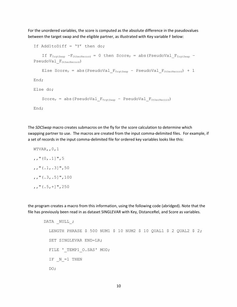
For the unordered variables, the score is computed as the absolute difference in the pseudovalues

between the target swap and the eligible partner, as illustrated with Key variable F below:

If Add1toDiff = ‘Y’ then do;

If FTrgtSwap –FOtherRecord = 0 then ScoreF = abs(PseudoVal_FTrgtSwap –

PseudoVal_FOtherRecord)

Else ScoreF = abs(PseudoVal_FTrgtSwap – PseudoVal_FOtherRecord) + 1

End;

Else do;

ScoreF = abs(PseudoVal_FTrgtSwap – PseudoVal_FOtherRecord)

End;

The SDCSwap macro creates submacros on the fly for the score calculation to determine which

swapping partner to use. The macros are created from the input comma-delimited files. For example, if

a set of records in the input comma-delimited file for ordered key variables looks like this:

WTVAR,,0,1

,,"(0,.1]",5

,,"(.1,.3]",50

,,"(.3,.5]",100

,,"(.5,+]",250

the program creates a macro from this information, using the following code (abridged). Note that the

file has previously been read in as dataset SINGLEVAR with Key, DistanceRel, and Score as variables.

DATA _NULL_;

LENGTH PHRASE $ 500 NUM1 $ 10 NUM2 $ 10 QUAL1 $ 2 QUAL2 $ 2;

SET SINGLEVAR END=LR;

FILE '_TEMP1_O.SAS' MOD;

IF _N_=1 THEN

DO;

11

PHRASE='%MACRO O_'||TRIM(LEFT(KeyVariable))||'

(PREFIX=,PREFIX2=);';

PUT PHRASE;

END;

NUM1=SCAN(DistanceRel,1,',([)]');

NUM2=SCAN(DistanceRel,2,',([)]');

IF NUM2='+' THEN

DO;

IF SUBSTR(DistanceRel,1,1)='(' THEN QUAL2='>';

ELSE IF SUBSTR(DistanceRel,1,1)='[' THEN QUAL2='>=';

PHRASE=' IF '||

'ABS(('||'&PREFIX2.'||TRIM(LEFT(KeyVariable))||' - '||

'&PREFIX.'||TRIM(LEFT(KeyVariable))||')/'||

'&PREFIX2.'||TRIM(LEFT(KeyVariable))||') '||

QUAL2||' '||TRIM(LEFT(NUM1))||

' THEN Score_'||TRIM(LEFT(KeyVariable))||' =

'||PUT(Score,8.)||';';

PUT PHRASE;

END;

ELSE

DO;

IF SUBSTR(DistanceRel,1,1)='(' THEN QUAL1='<';

ELSE IF SUBSTR(DistanceRel,1,1)='[' THEN QUAL1='<=';

IF INDEX(DistanceRel,')') > 0 THEN QUAL2='<';

ELSE IF INDEX(DistanceRel,']') > 0 THEN QUAL2='<=';

PHRASE=' IF '||TRIM(LEFT(NUM1))||' '||QUAL1||

'ABS(('||'&PREFIX2.'||TRIM(LEFT(KeyVariable))||' - '||

12

'&PREFIX.'||TRIM(LEFT(KeyVariable))||')/'||

'&PREFIX2.'||TRIM(LEFT(KeyVariable))||') '||

QUAL2||' '||TRIM(LEFT(NUM2))||

‘ THEN Score_'||TRIM(LEFT(KeyVariable))||' = '||

PUT(Score,8.)||';';

PUT PHRASE;

END;

IF LR THEN

DO;

PHRASE='%MEND O_'||TRIM(LEFT(KeyVariable))||';';

PUT PHRASE / ' ';

END;

RUN;

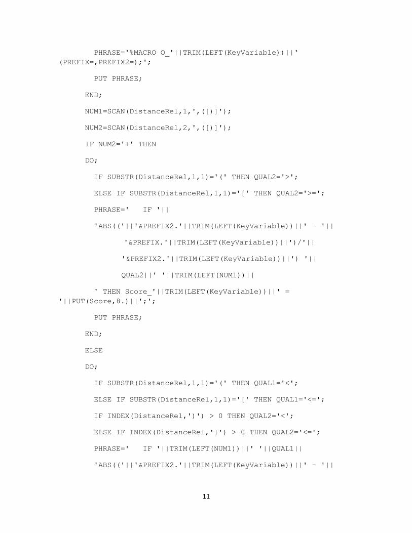
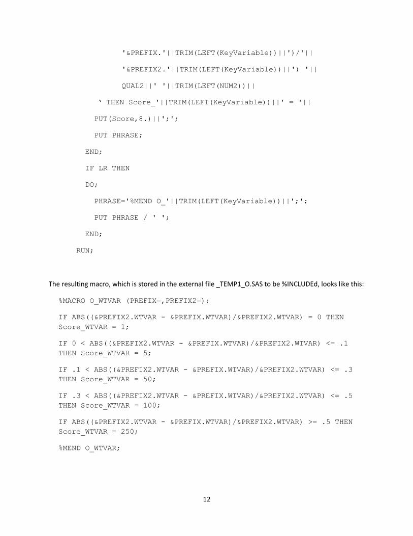
The resulting macro, which is stored in the external file _TEMP1_O.SAS to be %INCLUDEd, looks like this:

%MACRO O_WTVAR (PREFIX=,PREFIX2=);

IF ABS((&PREFIX2.WTVAR - &PREFIX.WTVAR)/&PREFIX2.WTVAR) = 0 THEN

Score_WTVAR = 1;

IF 0 < ABS((&PREFIX2.WTVAR - &PREFIX.WTVAR)/&PREFIX2.WTVAR) <= .1

THEN Score_WTVAR = 5;

IF .1 < ABS((&PREFIX2.WTVAR - &PREFIX.WTVAR)/&PREFIX2.WTVAR) <= .3

THEN Score_WTVAR = 50;

IF .3 < ABS((&PREFIX2.WTVAR - &PREFIX.WTVAR)/&PREFIX2.WTVAR) <= .5

THEN Score_WTVAR = 100;

IF ABS((&PREFIX2.WTVAR - &PREFIX.WTVAR)/&PREFIX2.WTVAR) >= .5 THEN

Score_WTVAR = 250;

%MEND O_WTVAR;

13

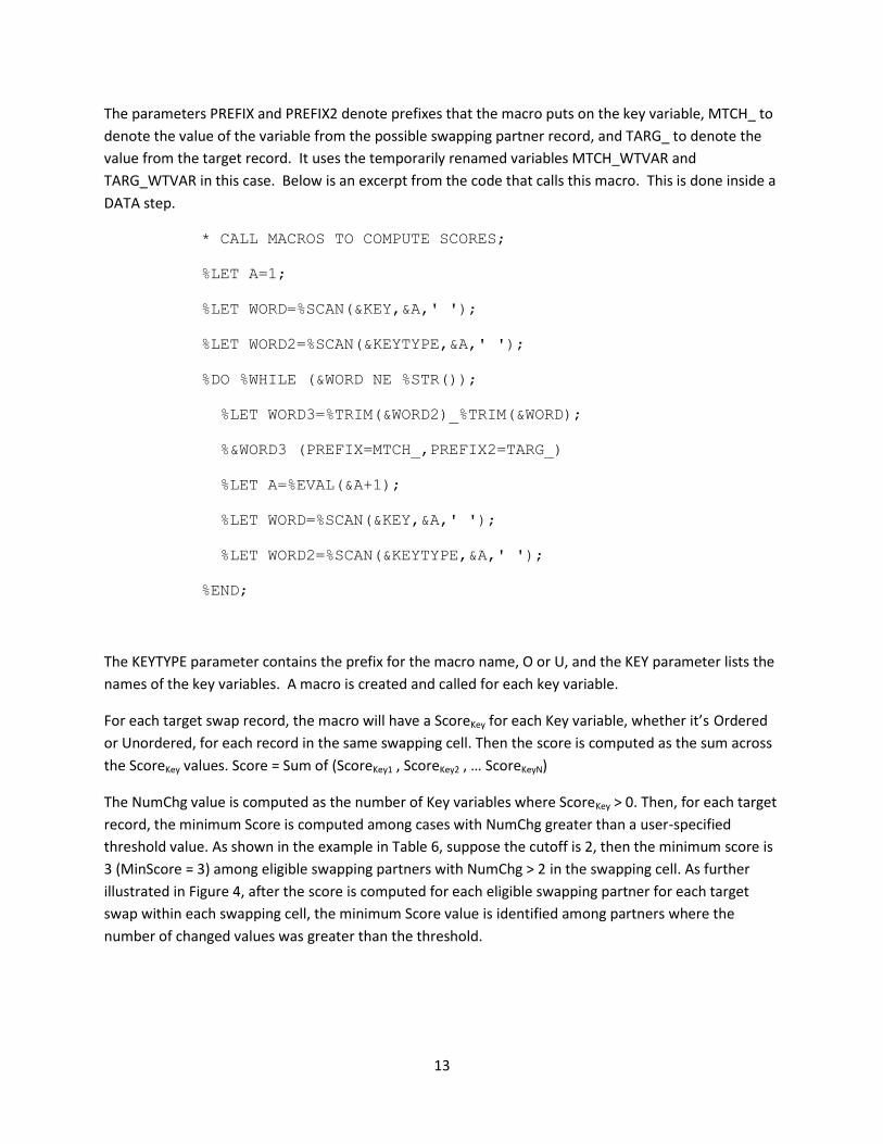
The parameters PREFIX and PREFIX2 denote prefixes that the macro puts on the key variable, MTCH_ to

denote the value of the variable from the possible swapping partner record, and TARG_ to denote the

value from the target record. It uses the temporarily renamed variables MTCH_WTVAR and

TARG_WTVAR in this case. Below is an excerpt from the code that calls this macro. This is done inside a

DATA step.

* CALL MACROS TO COMPUTE SCORES;

%LET A=1;

%LET WORD=%SCAN(&KEY,&A,' ');

%LET WORD2=%SCAN(&KEYTYPE,&A,' ');

%DO %WHILE (&WORD NE %STR());

%LET WORD3=%TRIM(&WORD2)_%TRIM(&WORD);

%&WORD3 (PREFIX=MTCH_,PREFIX2=TARG_)

%LET A=%EVAL(&A+1);

%LET WORD=%SCAN(&KEY,&A,' ');

%LET WORD2=%SCAN(&KEYTYPE,&A,' ');

%END;

The KEYTYPE parameter contains the prefix for the macro name, O or U, and the KEY parameter lists the

names of the key variables. A macro is created and called for each key variable.

For each target swap record, the macro will have a ScoreKey for each Key variable, whether it’s Ordered

or Unordered, for each record in the same swapping cell. Then the score is computed as the sum across

the ScoreKey values. Score = Sum of (ScoreKey1 , ScoreKey2 , … ScoreKeyN)

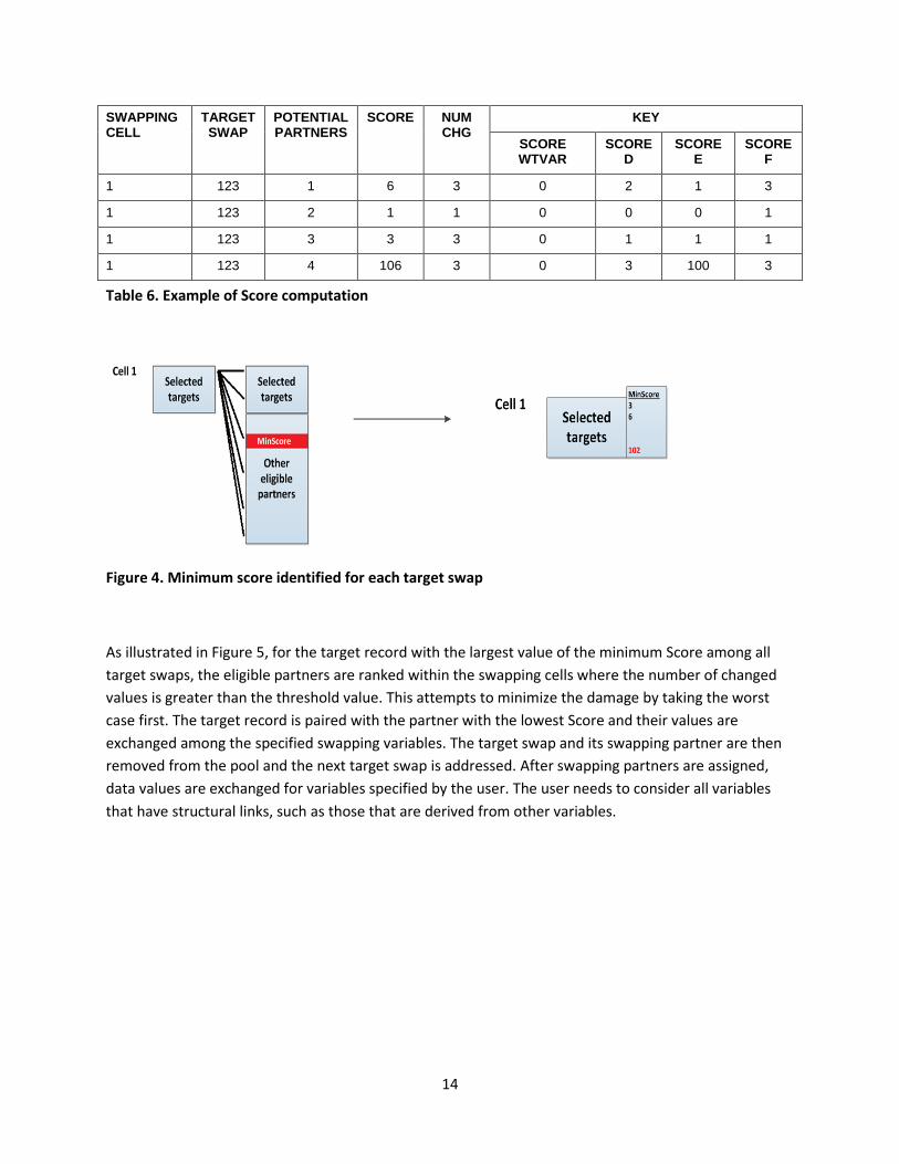
The NumChg value is computed as the number of Key variables where ScoreKey > 0. Then, for each target

record, the minimum Score is computed among cases with NumChg greater than a user-specified

threshold value. As shown in the example in Table 6, suppose the cutoff is 2, then the minimum score is

3 (MinScore = 3) among eligible swapping partners with NumChg > 2 in the swapping cell. As further

illustrated in Figure 4, after the score is computed for each eligible swapping partner for each target

swap within each swapping cell, the minimum Score value is identified among partners where the

number of changed values was greater than the threshold.

14

SWAPPING CELL

TARGET SWAP

POTENTIAL PARTNERS

SCORE NUM CHG

KEY

SCORE WTVAR

SCORE D

SCORE E

SCORE F

1 123 1 6 3 0 2 1 3

1 123 2 1 1 0 0 0 1

1 123 3 3 3 0 1 1 1

1 123 4 106 3 0 3 100 3

Table 6. Example of Score computation

Figure 4. Minimum score identified for each target swap

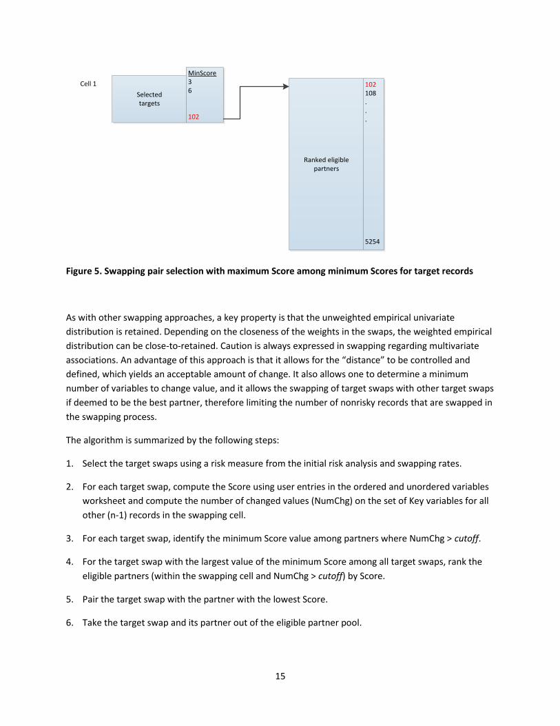
As illustrated in Figure 5, for the target record with the largest value of the minimum Score among all

target swaps, the eligible partners are ranked within the swapping cells where the number of changed

values is greater than the threshold value. This attempts to minimize the damage by taking the worst

case first. The target record is paired with the partner with the lowest Score and their values are

exchanged among the specified swapping variables. The target swap and its swapping partner are then

removed from the pool and the next target swap is addressed. After swapping partners are assigned,

data values are exchanged for variables specified by the user. The user needs to consider all variables

that have structural links, such as those that are derived from other variables.

15

Selectedtargets

MinScore36

102

Ranked eligible partners

Cell 1 102108...

5254

Figure 5. Swapping pair selection with maximum Score among minimum Scores for target records

As with other swapping approaches, a key property is that the unweighted empirical univariate

distribution is retained. Depending on the closeness of the weights in the swaps, the weighted empirical

distribution can be close-to-retained. Caution is always expressed in swapping regarding multivariate

associations. An advantage of this approach is that it allows for the “distance” to be controlled and

defined, which yields an acceptable amount of change. It also allows one to determine a minimum

number of variables to change value, and it allows the swapping of target swaps with other target swaps

if deemed to be the best partner, therefore limiting the number of nonrisky records that are swapped in

the swapping process.

The algorithm is summarized by the following steps:

1. Select the target swaps using a risk measure from the initial risk analysis and swapping rates.

2. For each target swap, compute the Score using user entries in the ordered and unordered variables

worksheet and compute the number of changed values (NumChg) on the set of Key variables for all

other (n-1) records in the swapping cell.

3. For each target swap, identify the minimum Score value among partners where NumChg > cutoff.

4. For the target swap with the largest value of the minimum Score among all target swaps, rank the

eligible partners (within the swapping cell and NumChg > cutoff) by Score.

5. Pair the target swap with the partner with the lowest Score.

6. Take the target swap and its partner out of the eligible partner pool.

16

7. Go to the next target swap.

8. If last target swap in cell, then go to next cell and repeat.

9. Exchange values of variables in the list of swapping variables.

10. Assign change flags to identify changed values.

SUMMARY

This paper summarized algorithms for two key components of the SDC process, namely data coarsening

and data swapping. To improve efficiency, the algorithms were implemented within a standardized suite

of SAS macros. The resulting software essentially standardized approaches used within the organization

and reduced processing time under increasing demands for data. While the macros are proprietary,

select code snippets of challenging parts of the program have been included. These challenges include

assigning formats for recodes and computing scores for target swap records and their potential

swapping partners.

REFERENCES

Dalenius, T. and Reiss, S. (1982). Data-swapping: A technique for disclosure control. Journal of Statistical

Planning and Inference, 6, 73–85.

Elliot, M., Manning, A., and Ford, R. (2002). A computational algorithm for handling the special uniques

problem. International Journal of Uncertainty, Fuzziness and Knowledge Based System, Vol 10, No. 5,

pp 493–509.

FCSM (2005). Report on Statistical Disclosure Methodology. Statistical Policy Working Paper 22 of the

Federal Committee on Statistical Methodology, 2ndversion. Revised by Confidentiality and Data

Access Committee 2005, Statistical and Science Policy, Office of Information and Regulatory Affairs,

Office of Management and Budget. http://www.fcsm.gov/working-papers/SPWP22_rev.pdf (current

as of October 21, 2012).

Fienberg, S. and McIntyre, J. (2005). Data Swapping: Variations on a Theme by Dalenius and Reiss.

Journal of Official Statistics, 21, No. 2.

Hundepool, A., Domingo-Ferrer, J., Franconi, L., Giessing, S., Nordholt, E. S., Spicer, K. and de Wolf, P.-P.

(2012). Data Access Issues, in Statistical Disclosure Control, John Wiley & Sons, Ltd, Chichester, UK.

doi: 10.1002/9781118348239.ch6

Kaufman, S., Seastrom, M., and Roey, S. (2005). Do disclosure controls to protect confidentiality degrade

the quality of the data? Proceedings of the Joint Statistical Meetings, American Statistical

Association Section on Government Statistics. Alexandria, VA: American Statistical Association.

Li, J. and Krenzke, T. (2013). Comparing Approaches That Are Used to Identify High Risk Values in

Microdata Census Statistical Disclosure Control Research Project 3. Final Report. July 29, 2013. U.S.

Bureau of the Census, Washington, D.C.

Ramanayake, A. and Zayatz, L. (2010). Balancing disclosure risk with data quality. Research Report Series

(Statistics #2010-04). Statistical Research Division, U.S. Census Bureau, Washington, D.C.

17

Woo, M., Reiter, J., Oganian, A. and Karr, A. (2009). Global measures of data utility for microdata

masked for disclosure limitation. The Journal of Privacy and Confidentiality. 1, Number 1, pp. 111-

124.

CONTACT INFORMATION

Your comments and questions are valued and encouraged. Contact the author at:

Name: Tom Krenzke

Organization: Westat

Address: 1600 Research Boulevard

City, State ZIP: Rockville MD, 20850

Work Phone: (301) 251-4203

Fax: 301-294-2034

Email: krenzkt1@westat.com

SAS and all other SAS Institute, Inc. product or service names are registered trademarks or trademarks

of SAS Institute, Inc. in the USA and other countries. ® indicates USA registration.

Other brand and product names are trademarks of their respective companies.

18

APPENDIX

SELECT PARAMETERS FROM SDCCOARSEN AND SDCSWAP

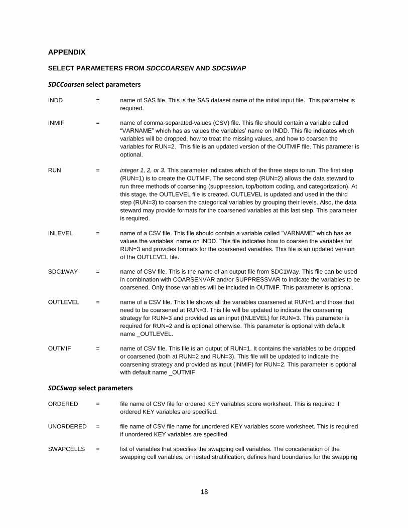
SDCCoarsen select parameters

INDD = name of SAS file. This is the SAS dataset name of the initial input file. This parameter is

required.

INMIF = name of comma-separated-values (CSV) file. This file should contain a variable called

“VARNAME” which has as values the variables’ name on INDD. This file indicates which

variables will be dropped, how to treat the missing values, and how to coarsen the

variables for RUN=2. This file is an updated version of the OUTMIF file. This parameter is

optional.

RUN = integer 1, 2, or 3. This parameter indicates which of the three steps to run. The first step

(RUN=1) is to create the OUTMIF. The second step (RUN=2) allows the data steward to

run three methods of coarsening (suppression, top/bottom coding, and categorization). At

this stage, the OUTLEVEL file is created. OUTLEVEL is updated and used in the third

step (RUN=3) to coarsen the categorical variables by grouping their levels. Also, the data

steward may provide formats for the coarsened variables at this last step. This parameter

is required.

INLEVEL = name of a CSV file. This file should contain a variable called “VARNAME” which has as

values the variables’ name on INDD. This file indicates how to coarsen the variables for

RUN=3 and provides formats for the coarsened variables. This file is an updated version

of the OUTLEVEL file.

SDC1WAY = name of CSV file. This is the name of an output file from SDC1Way. This file can be used

in combination with COARSENVAR and/or SUPPRESSVAR to indicate the variables to be

coarsened. Only those variables will be included in OUTMIF. This parameter is optional.

OUTLEVEL = name of a CSV file. This file shows all the variables coarsened at RUN=1 and those that

need to be coarsened at RUN=3. This file will be updated to indicate the coarsening

strategy for RUN=3 and provided as an input (INLEVEL) for RUN=3. This parameter is

required for RUN=2 and is optional otherwise. This parameter is optional with default

name _OUTLEVEL.

OUTMIF = name of CSV file. This file is an output of RUN=1. It contains the variables to be dropped

or coarsened (both at RUN=2 and RUN=3). This file will be updated to indicate the

coarsening strategy and provided as input (INMIF) for RUN=2. This parameter is optional

with default name _OUTMIF.

SDCSwap select parameters

ORDERED = file name of CSV file for ordered KEY variables score worksheet. This is required if

ordered KEY variables are specified.

UNORDERED = file name of CSV file name for unordered KEY variables score worksheet. This is required

if unordered KEY variables are specified.

SWAPCELLS = list of variables that specifies the swapping cell variables. The concatenation of the

swapping cell variables, or nested stratification, defines hard boundaries for the swapping

19

process and the search for swapping partners. The variables need to be space-delimited.

The parameter is required.

KEY = list of variables that specifies key matching variables for computing the score to measure

the distance between the target and partner. Each variable that is listed needs to have a

corresponding entry in the scoresheet ORDERED or UNORDERED, depending on the

variable type. The variables need to be space-delimited. The parameter is required.

KEYTYPE = a list of O/U, one for each KEY variable: Ordered (O) Unordered (U). The list of Os and/or

Us is delimited by a space.

SWAPVARS = list of variables that specifies the swapping variables. Once the swapping partners are

found, the values of SWAPVARS variables are swapped between the target records and

their corresponding swapping partners. The parameter is required.

SWAPVARSTYPE= a list of O/U, one for each SWAPVARS variable: Ordered (O) Unordered (U). The list of

Os and/or Us is delimited by a space.

CUTOFF = a value, which determines the partner eligibility threshold based on the number of KEY

variables that are different between target and partner. The value needs to be greater than

CUTOFF for the data record to be considered as an eligible partner.