DATA ANALYSIS OF COMPLEX SYSTEMS - Defense ... ANALYSIS OF COMPLEX SYSTEMS June 2011 FINAL TECHNICAL...

APPROVED FOR PUBLIC RELEASE; DISTRIBUTION UNLIMITED.

STINFO COPY

AIR FORCE RESEARCH LABORATORY INFORMATION DIRECTORATE

DATA ANALYSIS OF COMPLEX SYSTEMS

June 2011 FINAL TECHNICAL REPORT

ROME, NY 13441 UNITED STATES AIR FORCE AIR FORCE MATERIEL COMMAND

AFRL-RI-RS-TR-2011-146

NOTICE AND SIGNATURE PAGE Using Government drawings, specifications, or other data included in this document for any purpose other than Government procurement does not in any way obligate the U.S. Government. The fact that the Government formulated or supplied the drawings, specifications, or other data does not license the holder or any other person or corporation; or convey any rights or permission to manufacture, use, or sell any patented invention that may relate to them. This report was cleared for public release by the 88th ABW, Wright-Patterson AFB Public Affairs Office and is available to the general public, including foreign nationals. Copies may be obtained from the Defense Technical Information Center (DTIC) (http://www.dtic.mil). AFRL-RI-RS-TR-2011-146 HAS BEEN REVIEWED AND IS APPROVED FOR PUBLICATION IN ACCORDANCE WITH ASSIGNED DISTRIBUTION STATEMENT. FOR THE DIRECTOR: /s/ /s/ CHARLES G. MESSENGER , Chief MICHAEL J. WESSING, Acting Chief Information Understanding Branch Information & Intelligence Exploitation Division Information Directorate This report is published in the interest of scientific and technical information exchange, and its publication does not constitute the Government’s approval or disapproval of its ideas or findings.

REPORT DOCUMENTATION PAGE Form Approved OMB No. 0704-0188

Public reporting burden for this collection of information is estimated to average 1 hour per response, including the time for reviewing instructions, searching data sources, gathering and maintaining the data needed, and completing and reviewing the collection of information. Send comments regarding this burden estimate or any other aspect of this collection of information, including suggestions for reducing this burden to Washington Headquarters Service, Directorate for Information Operations and Reports, 1215 Jefferson Davis Highway, Suite 1204, Arlington, VA 22202-4302, and to the Office of Management and Budget, Paperwork Reduction Project (0704-0188) Washington, DC 20503. PLEASE DO NOT RETURN YOUR FORM TO THE ABOVE ADDRESS.1. REPORT DATE (DD-MM-YYYY)

June 2011 2. REPORT TYPE

Final In-House Technical Report 3. DATES COVERED (From - To)

July 2009 – December 2010 4. TITLE AND SUBTITLE DATA ANALYSIS OF COMPLEX SYSTEMS

5a. CONTRACT NUMBER In House

5b. GRANT NUMBER N/A

5c. PROGRAM ELEMENT NUMBER62702F

6. AUTHOR(S) Misty K. Blowers

5d. PROJECT NUMBER 459E

5e. TASK NUMBER IH

5f. WORK UNIT NUMBER 07

7. PERFORMING ORGANIZATION NAME(S) AND ADDRESS(ES)Air Force Research Laboratory/Information Directorate Rome Research Site/RIED 525 Brooks Road Rome, NY 13441-4505

8. PERFORMING ORGANIZATION REPORT NUMBER N/A

9. SPONSORING/MONITORING AGENCY NAME(S) AND ADDRESS(ES)Air Force Research Laboratory/Information Directorate Rome Research Site 26 Electronic Parkway Rome NY 13441

10. SPONSOR/MONITOR'S ACRONYM(S) AFRL/RI

11. SPONSORING/MONITORING AGENCY REPORT NUMBER AFRL-RI-RS-TR-2011-146

12. DISTRIBUTION AVAILABILITY STATEMENT Approved for Public Release; Distribution Unlimited. PA# 88ABW-2011-3174 Date Cleared: June 2011

13. SUPPLEMENTARY NOTES

14. ABSTRACT The goal of this research effort is to investigate methods to fuse vast amounts of data coming from different sensor sources with amulti-layered semi-supervised learning approach. This approach will use basic statistical techniques to identify key predictors,some correlation techniques to validate the source, quality and temporal aspects of the data, artificial neural networks for troubleshooting sources of system variability, and semi-supervised learning techniques which will provide adjustable thresholds for forecasting and detecting various anomalies or events of interest.

15. SUBJECT TERMS Semi-Supervised Learning, K-Means, Pattern Matching, Anomaly Detection, Event Prediction, Artificial Neural Networks, Clustering, Threat Awareness

16. SECURITY CLASSIFICATION OF: 17. LIMITATION OF ABSTRACT

UU

18. NUMBER OF PAGES

100

19a. NAME OF RESPONSIBLE PERSON MISTY K. BLOWERS

a. REPORT U

b. ABSTRACT U

c. THIS PAGE U

19b. TELEPHONE NUMBER (Include area code) N/A

Standard Form 298 (Rev. 8-98) Prescribed by ANSI Std. Z39.18

Table of Contents

LIST OF FIGURES .......................................................................................................... iii

LIST OF TABLES ............................................................................................................ iv

1 EXECUTIVE SUMMARY .......................................................................................... 1

2 INTRODUCTION ........................................................................................................ 3

2.1 Motivation ........................................................................................................... 3 2.2 Overview of the Secondary Fiber Recovery System .......................................... 8 2.3 Sources of Variability in Fiber Recovery Process ............................................ 11 2.4 Data Collection ................................................................................................. 12 2.5 Basics of Process Control ................................................................................. 13 2.6 Multivariable System ........................................................................................ 17

3 MACHINE LEARNING (ML) ................................................................................... 19

3.1 Supervised Learning ......................................................................................... 19 3.1.1 Artificial Neural Networks ......................................................................... 19

3.2 Unsupervised Learning ..................................................................................... 23 3.2.1 Clustering................................................................................................... 24

3.3 Prior Applications of ML Algorithms in Industrial Process Systems............... 28 3.3.1 Applications of Artificial Neural Networks ................................................ 28 3.3.2 Applications of Clustering Algorithms ....................................................... 29 3.3.3 Applications Incorporating Fuzzy Logic into ML ...................................... 31

3.4 Choosing the Best Model .................................................................................. 32

4 DATA PREPROCESSING ......................................................................................... 33

4.1 Operator Interviews .......................................................................................... 33 4.2 Establishing Ground Truth ................................................................................ 34 4.3 Adjusting for Time Lags ................................................................................... 35

5 ANN’S FOR TROUBLESHOOTING PROCESS VARIABILITY ........................... 37

5.1 Choosing a Neural Network Model .................................................................. 40 5.2 Sensitivity Analysis .......................................................................................... 43 5.3 Optimizing the Neural Network Model ............................................................ 45 5.4 Conclusions ....................................................................................................... 46

6 PATTERN MATCHING TOOLS FOR EVENT PREDICTION .............................. 48

6.1 Background ....................................................................................................... 48 6.2 Data Preprocessing............................................................................................ 50 6.3 Mean Vector Distance ....................................................................................... 51 6.4 K-Nearest Neighbor .......................................................................................... 53 6.5 Modified K-Means Algorithm .......................................................................... 54 6.5.1 Modifications to the Java ML Toolkit ........................................................ 55 6.5.2 Cluster Evaluation ....................................................................................... 56 6.5.3 Semi-Fuzzy K-Means ................................................................................. 58

i

6.5.4 Quality Threshold K-Means ....................................................................... 62 6.6 Summary ........................................................................................................... 69

7 ADDITIONAL PREDICTION TOOLS AND ANALYSIS....................................... 72

7.1 Detecting rate of change ................................................................................... 72 7.2 Analysis of Operator Response ......................................................................... 74 7.3 Conclusions ....................................................................................................... 75

8 CONCLUSIONS AND FUTURE DIRECTION ........................................................ 76

8.1 Conclusions ....................................................................................................... 76 8.2 Future Direction ................................................................................................ 78 8.2.1 Basic Research ............................................................................................ 78 8.2.2 Applied Research ........................................................................................ 78

9 BACK MATTER ........................................................................................................ 80

9.1 Appendix A - Java-ML Method For Accessing Centroids ............................... 80 9.2 Appendix B - Detecting Rate Of Change Prior To Paper Break Occurances ... 84 9.3 List of Acronyms .............................................................................................. 86

10 BIBLIOGRAPHY ....................................................................................................... 87

11 PUBLICATIONS ........................................................................................................ 93

ii

List of Figures Figure 1 The industrial process is a complex system with many sensor points. ...................................... 3 Figure 2 A simplified flow diagram of the third Paper Machine (PM3) secondary fiber line at the

Rock -Tenn Paper Mill illustrates the complexity of the industrial test bed. .............................. 10 Figure 3 A simplified illustration of the neural network training mechanism. The network is

adjusted based on a comparison of the output and the target until the network output matches, or nearly matches, the target. .......................................................................................................... 20

Figure 4 Within a single input neuron the scalar input, p, is multiplied by the scalar weight, w, to form wp, which is one of the terms that is sent to the summer. If the neuron includes a bias it is also passed to the summer. The net input, n, goes to the transfer function, f, which produces the scalar neuron output, a. .............................................................................................................. 21

Figure 5 A multiple input neuron inputs p1, p2, …pr are each weighted by corresponding elements w1,1, w1,2,….w1,R of the weight matrix W. ................................................................................... 21

Figure 6 Example of a three-layer artificial neural network. Each layer has its own weight matrix, its own bias vector, and net input vectors. Internal layers are often hidden to simplify the model (44). ..................................................................................................................................................... 22

Figure 7 The Ensemble Neural Network Model is a stack of many neural networks with the same complexity. An advantage of this approach is that the final prediction is based on the average of all models in the ensemble. ........................................................................................................... 23

Figure 8 The K-means algorithm is an example of a partitioning method. This illustration shows how it can be used to finds three clusters in a sample of data. .............................................................. 26

Figure 9 The design cycle for complex system analysis (58). The characteristics of the data affect the selection of the best features and the best model. The training process uses some or all of the data to determine the best system parameters. After evaluating the models performance, it may be necessary to repeat various steps in the design process to improve the results. ............. 32

Figure 10 The graph shows the linear relationship of some highly correlated variables over a three day time period. ................................................................................................................................. 37

Figure 11 Neural network prediction results with no filtering of the data ............................................ 42 Figure 12Neural Network improved just by filtering outliers in the data ............................................. 42 Figure 13 The results from the sensitivity analysis shows that the five highest correlated variables

included: the secondary refiner accept recirculation line, the disc thickener, the primary course screen accept flow line, the primary course screen consistency value, and the couch vacuum. . 44

Figure 14 Predictive performance is degraded when the output as a predictor is removed from the inputs. ................................................................................................................................................. 44

Figure 15 When data regimes are separated and considered separately the neural network performance improves. ..................................................................................................................... 45

Figure 16 Cluster Evaluator for 6 months of data shows that 10 clusters should be the initial value for K. .................................................................................................................................................. 57

Figure 17 Fuzzy K-Means GUI displays specified clusters and cluster sizes ....................................... 59 Figure 18 When implementing QT K-Means Model One clusters are formed around the fault

indicating records. The size of the cluster is adjusted by changing the threshold value. ........... 63 Figure 19 GUI for QT-K-Means model one shows how the threshold values of each cluster can be

adjusted in the training set to improve prediction accuracy. ........................................................ 64 Figure 20 Red line shows L2 distance from t-5 to t for each 25 minutes of time. The blue line shows

Paper Machine Breaks. .................................................................................................................... 84 Figure 21 Red line shows L2 distance from t-5 to t for each 25 minutes of time. The blue line shows

Paper Machine Breaks. .................................................................................................................... 85

iii

List of Tables Table 1 Major paper grades classification (15) .......................................................................................... 8 Table 2 Various sensors and corresponding tag numbers of interest at the recycle paper mill in

Solvay, NY. ........................................................................................................................................ 16 Table 3 The table shows the magnitude of the discrepancies in the raw data when using the steam

values as an indicator of paper machine status verses using the operator logs. .......................... 34 Table 4 Time lags from paper machine of various equipment sensors. ................................................. 36 Table 5 Comparison of Mill’s Recommended Lag Times (min) to Spearman’s Analysis ................... 39 Table 6 Correlation of variables to the couch vacuum section of PM 3. ............................................... 39 Table 7 Backpropagation Neural Network Application Comparison Chart ........................................ 40 Table 8 Comparison of Backpropagation Network to the Ensemble Model ........................................ 41 Table 9 Comparison of Network Results with Single Variable Inputs .................................................. 46 Table 10 T-Test Highest Values indicate the variables with most class differentiation ....................... 50 Table 11 Variables with largest difference in mean between two classes .............................................. 51 Table 12 Results from Mean Vector Distance Algorithm (shown as percentages) .............................. 52 Table 13 MVD model failed to give consistent results (shown as percentages). .................................... 52 Table 14 Comparison of performance of L1, L2 distance functions and data sets on KNN (shown as

percentages). ...................................................................................................................................... 54 Table 15 Comparison of performance of L1, L2 distance functions and data sets on Semi-Fuzzy K-

Means (shown as percentages) ......................................................................................................... 59 Table 16 Comparison of performance of Semi-Fuzzy K-Means over subsequent train/testing sets

(shown as percentages). .................................................................................................................... 60 Table 17 Example of implementation of the semi-fuzzy k-means model ............................................... 60 Table 18 Comparison of performance of L1, L2 distance functions and data sets on Q-T K-means

Model One (shown in percentages). ................................................................................................. 65 Table 19 the QT K-Means Model allows for the mapping of Operator Log to clusters ...................... 66 Table 20 The breakdown of performance per cluster with low sensitivity ............................................ 67 Table 21 The breakdown of performance per cluster when the sensitivity is increased ...................... 67 Table 22 QTM1 gave repeatable results at low sensitivity values. ......................................................... 68 Table 23 Threshold values for low sensitivity QTM1 .............................................................................. 68 Table 24 QTM1 gave repeatable results at higher sensitivity values. .................................................... 68 Table 25 Threshold values for high sensitivity QTM1 ........................................................................... 68 Table 26 Comparison of performance of L1, L2 distance functions and data sets on Q-T K-means

Model Two ......................................................................................................................................... 69 Table 27 Summary of results of Models Investigated............................................................................. 70 Table 28 There were benefits and limitations to each model investigated. ............................................ 71 Table 29 Frequency of the changes that occurred with each binning of L2 distance values ............... 73 Table 30 The table above shows the count on the number of times the operator made changes to the

status of the control loops. ................................................................................................................ 75 Table 31 Cost Benefit for various failure detection performances ........................................................ 77

iv

1 EXECUTIVE SUMMARY There are numerous applications across the Department of Defense where there are a number of sensor inputs to be considered and massive amounts of data to be processed in order for an operator or analyst to determine if an abnormal condition or event of interest is about to occur. The goal of this research effort is to investigate methods to fuse these vast amounts of data coming from these different sensor sources with a multi-layered semi-supervised learning approach. This approach will use basic statistical techniques to identify key predictors, some correlation techniques to validate the source, quality and temporal aspects of the data, artificial neural networks for troubleshooting sources of system variability, and semi-supervised learning techniques which will provide adjustable thresholds for forecasting and detecting various anomalies or events of interest.

The outputs from the machine learning algorithms investigated in this research effort can provide critical information for operators and analysts. This information could allow the operators to make proactive decisions to potentially prevent and/or prepare for a hazardous (or costly) event. However, in order for many machine learning methods to be successful, an iterative design analysis, combined with domain expertise, is important in identifying the appropriate inputs to the algorithm. A precaution should be taken not to reduce the performance of the algorithm by adding “noisy” data.

For rapid situation awareness for the analyst, a robust assessment of these sensor inputs is necessary. These sensor measurements can be assembled into a vector, so the entire vector represents an observation from a multivariate population. When applied to a real world multi-sensor environment, the operation and internal complexity becomes represented in terms of the collection of vectors which describe the different observations, or states, of the overall domain specific space (battlespace, airspace, etc) at different points in time. The value of each point represents a measured variable from the various sensors. A feature vector is an n-dimensional vector of numerical features that come from the various sensor points. The problem in dealing with real world data sets is that the number of anomalies contained within the data is drastically disproportionate from the amount of normalcy. In order for the system to be robust enough to handle a real world situation, the learning method used must be able to account for the lack of data in times of anomalous conditions as well as the overlap in periods of abnormality and normalcy.

The work for this project was divided into the following major areas:

Correlation and Statistical Analysis

One of the simplest of the feature selection process is a modification of the Tukey Test (t-test). The Tukey Test is a simple statistical test that can be used to identify the features which vary the most between subsets of the various classes. Correlation methods like Spearman’s rank correlation will be evaluated to for further analysis of the features selected from the process described above. Spearman’s rank correlation is a

Approved for Public Release; Distribution Unlimited 1

nonparametric (nonlinear) correlation analysis which may be used to determine the correlation of each proposed input variable to the output variable (Xi, Yi).

Next, an Artificial Neural Network (ANN) model combined with a subsequent sensitivity analysis is evaluated. A neural network proved successful in this application for identifying the sources of variability on the predicted output value. This chapter will discuss how choosing the most appropriate ANN and model inputs helped improve prediction accuracy.

Semi-Supervised Machine Learning Algorithms

Semi-Supervised machine learning models were investigated with the JAVA_ML toolkit. These include a simple mean vector distance model, K-Nearest Neighbor, and some modified K-Means models. These models were used to predict events of interest.

The mean vector distance model uses a rather simple mean vector codebook in order to characterize the mean of normalcy and anomalous conditions. This method had its limitations in that in complex systems there can be many modes of operation for each class. This led to the next area of investigation in which the model searched for multiple means (K-Means) of vectors. A Semi-Fuzzy K-Means algorithm was developed which explored the clusters formed by both times of normalcy and abnormality and used the probability of membership into each to make a prediction on when an anomalous event was about to occur.

Another modification to the standard K-Means model was the Quality Threshold Model (QTM), in which the sensitivity of the model could be adjusted by changing threshold values to accommodate the tolerance level the mill may have for false alarms verses the cost benefit from early detection. In order to understand what information the various clusters represented, the events from the operator logs were mapped to the clusters which were defined by fault indicator vectors.

Rate of Change Model and Test of Operator/Analyst Response

Backward Differencing is designed to detect rates of change from the current time step to a prior time step. A series of test and data analysis techniques where employed in order to understand more about the data and to determine whether anomalous vectors were preceded by some sort of quantifiable events. The rate of change model presented in this work is a simplification of backward differencing, but it has the same goal of trying to detect rates of change from one time step to the next. In addition to backward differencing, an analysis was performed to explore the effects of the operators’ response to system changes. This algorithm compares the number of operator changes that occur just prior to an event of interest occurring to the number of operator changes that occur when the system was running in a good operating mode.


2 INTRODUCTION

2.1 Motivation An unclassified data set was used in this research effort which was obtained from a manufacturing environment. There were numerous sensor locations throughout the process. Initially, 79 data points where considered as having some correlation to the events of interest. A simplified flow diagram illustrates where some of these sensor points were located.

Figure 1 The industrial process is a complex system with many sensor points. In addition to the numerous applications across the DoD that the methods contained in this research may benefit, the industrial domain investigated also may realize substantial gains. These tools may be used to minimize the amount of downtime for an industrial paper recycling mill. Downtime is caused by a number of factors, and this research exposes which components of a particular mill can be indicators of an upcoming failure. These factors can then be detected by an automated computer system in order to warn an operator prior to a paper machine break occurring. The dynamic industrial environment investigated had substantial variability in the incoming raw material. Variability in operating conditions in industrial processes has the potential to cause loss of production, damaged equipment, and could create an unsafe operating environment. Just like the military domain, when an upset condition occurs,

HD Cleaners

Pulper Dump Chest

Coarse Screens HD Cleaner FractionatorConveyor

Fine Screens

Washer

Disc Thickener

Storage chest

Couch vacuum (Vo)


the operators are inundated with huge amounts of data to be processed in a short amount of time. However, the cost of making a bad decision in an industrial setting is typically much lower. In industry, it is more typical that money, not lives, is what is lost. Industrial settings can be a creative place to develop tools to be used in other settings. One has access to unclassified, real world data, which is laden with noise and uncertainty. The automated computer system which could be fielded with the tools contained in this research, could serve as an indications and warnings system which could monitor and study processes during production. Such systems could not only advise the operators of the various actions to be taken to keep the processes running in a stable fashion, they could also minimize the probability of paper machine downtimes. Organizations within the paper industry have dedicated a significant amount of time and resources into promoting the development and application of modeling and simulation techniques in the paper industry as a whole (1). Some of the main objectives of studying these techniques are to reduce emissions and to increase the productivity and cost-efficiency of the process. The process of making pulp and paper includes many re-circulated streams of water, fibers, fillers, and air. For this reason, static models and balances can be very complex and tend to ignore the process dynamics. There have been very few publications which successfully demonstrate simulating the dynamics of pulp and paper machine systems. The dynamics of the paper machine wet end have been described as being an extremely complex combination of hydrodynamics and colloidal chemistry (1). In order to manage the dynamics of a paper recycling mill, complex process control systems have been widely established. The number of I/O connections in typical mills can vary from 30,000 to more than 100,000. The industry is constantly searching for ways to manage these complex systems in better ways. The first issue to be addressed is in how to handle the huge amount of raw sensor data available within the system. High-dimensional data analysis and reduction are important techniques used to help reduce the dimensionality of the huge of amount of raw data (1). From here, various process monitoring and simulation methods exist. These methods are typically either data driven, analytical, or knowledge based (2). Various techniques from modeling and simulation attempt to characterize the process behavior and are used to develop models for predicting how the system will respond during system upsets or equipment changes. Some research has shown that even small fluctuations in process signals may be precursors to predicting system upsets (2). It is important for an automated system to be able to distinguish the inherent variability of the process from the precursors to system upsets or faults. One of the biggest challenges in a system which has a great deal of inherent variability is to identify when, where, and how much change is significant. If a system cannot correctly identify the precursors to a failure state, the operators may be inundated with false alarms and lose faith in the reliability of the automated system.


For most minor process fluctuations the process controllers (Proportional, Integral, and Derivative (PID)) and model predictive controllers are designed to maintain satisfactory operations by compensating for the effects of disturbances and changes occurring in the process. However, there are some changes in the process which cause disturbances which the controllers cannot adequately handle. These are the disturbances may lead to faults (3) (4). Isermann (5) wrote a review article on fault detection based on modeling and system estimation. He claims that with a good model of the process, we can improve our ability to indicate when process faults are likely. As with other similar process models, his system compared current process signatures and outputs with those from the model. When values above or below some threshold were detected, they were labeled as fault indicators. The problem is that when the system is so complex and dynamic, models like Isermann's are often limited. Systems that are currently available rarely try to evaluate the process from the raw material through final product. More often, they try to break the process up into its subprocesses and in doing so, some dependencies may be overlooked. This is especially important when considering the amount of recirculated material within the system. Due to the interdependencies of the various processes in the system, along with the recirculation of material, tracing the time lags in the system also becomes an enormously challenging problem. Some research efforts have looked at inducing a model using time-series analysis. One classical approach is to build an autoregressive moving average (ARMA) (6). Often associated with the ARMA approach is the cumulative sum (CUSUM) of the residuals method to identify faults. Unfortunately, these methods are limited when the process has many modes of operation, or grades, which are produced in a single process (7). Research efforts, by Kim et al., have focused on monitoring various process signatures in real-time and incorporating these with equipment maintenance history data and in-line measurements of product quality (8). Combining information in this way helped build stronger process models and inspired some of the data analysis techniques presented in this research. To add to the overall difficulty of dealing with a complex system, uncertainty exists in the sensory measurements, there is cooperation among certain sensors, and there are competing objectives among other sensors. Basir et al. (3) presented a probabilistic approach for modeling the uncertainty and cooperation between sensors. Their research shows how measures of variation can be used to capture both the quality of sensory data and the interdependence relationships that might exist between the different sensors. Some methods presented in this work use information about the variance and standard deviation of each sensor to capture similar relationships in the process. Both within the paper industry, as well as in other manufacturing environments, various research efforts (9) (10) have explored using neural networks to model the process dynamics. Some research has demonstrated the ability of time-delay neural networks to


capture the dynamics of the process. Others (11) (8) have explored the possibility of knowledge based neural network models. The limitation in using neural network models is that the model may become overtrained for a given set of training inputs. When a neural network becomes overtrained, it has modeled the training set too closely and cannot correctly generalize to other inputs. Therefore, when process conditions change, retraining of the network model may be necessary. While such limitations need to be accounted for, neural network models can still be a very useful tool. This is especially evident when they are paired with other methods, like sensitivity analysis. A sensitivity analysis indicates which input variables are considered most important by a particular neural network. Sensitivity analysis can give important insights into the usefulness of individual variables (12). This research will show how a neural network model and the subsequent sensitivity analysis of a trained network can be crucial in identifying key sources of variability in the moisture on the wet end section of a paper machine, see Figure 1, Chapter 2. In processes where there is more than one grade being produced on a single paper machine, there becomes another challenge in dealing with different modes of operation. For this reason, clustering algorithms were explored. Clustering algorithms have the advantage of discovering multiple clusters of operating modes, allowing for the system to create multiple functions to describe modes of good or bad process conditions. Different paper mills may require different models to best characterize the complex process interactions. Different processes are going to have differences in time delays and natural process fluctuations. The purpose of this research is to explore some of the current data analysis techniques from the field of computer science, and show how they can be effectively used in a real world industrial process setting, more specifically for the purpose of identifying upcoming failure conditions in a paper recycling mill. Whatever method is used, the end user must give careful consideration as to what techniques are best suited for their process environment. The software system must have the ability to detect process upsets or anomalies soon enough for operators to react. The neural networks and clustering algorithms presented in this work are a step closer to helping operators and analyst deal with some of the challenges in modeling a complex system. The analysis presented in the exploratory chapters of this research effort is intended to offer some ideas and to direct future research efforts which explore operator response and ways of incorporating operator knowledge into a model.


The source company for the data used for this research manufactures containerboard for the corrugating industry. The data used for this research is specific to this industrial process, but similar data sets can be obtained from other industrial settings as long as there is a data collection and management infrastructure. The plant historian, or plant information system (PI system), in this industrial setting was supplied by OSIsoft. It is designed to gather and archive large volumes of data (13). The PI system is very commonly used in the pulp and paper industry.


2.2 Overview of the Secondary Fiber Recovery System A paper mill is an industrial environment which is dynamic and complex. Paper can be graded in 'm' numbers of ways (14). If we count all permutations and combinations of grades, the total grades may well exceed 10,000. Some of the different types of paper grades that are produced are shown in Table 1. Table 1 Major paper grades classification (15) Based on Basis Weight Tissue: Low weight, <40 g/m2

Paper: Medium weight, 40 - 120 g/m2

Paperboard: Medium High weight, 120-200 g/m2 Board: High weight, >200 g/m2

Based on Color Brown: Unbleached White: Bleached Colored: Bleached and dyed or pigmented

Based on Usage Industrial: Packaging, wrapping, filtering, electrical etc. Cultural: Writing, printing, Newspaper, currency etc. Food: Food wrapping, candy wrapping Coffee filter, tea bag etc.

Based on Raw Material Wood: Contain fibers from wood Agricultural residue: Fibers from straw, grass or other annual plants Recycled: Recycle or secondary Fiber

Based on Surface Treatment Coated: Coated with clay or other mineral. Uncoated: No coating Laminated: aluminum, poly etc

Finish Fine/Course calendered/ supercalendered Machine Finished (MF)/Machine Glazed (MG) Glazed/Glossed

One can imagine with all of the grades manufactured, there is a great deal of variability from one grade to the next. Even within a single grade, a great deal of variability exists. Reducing the variability of the process can lead to savings on raw material costs and reduce the variability of the final product. In turn, this can reduce the amount of offgrade product and reduce the number of paper machine breaks and subsequent lost production time. Software systems can offer many advantages to such a complex process environment. One key benefit is in identifying the sources of variability which then may be reduced by operators or automatically by computer systems. Another is by detecting when swings in process variability can act as precursor to help predict when a process failure or a paper machine break is likely to occur. Early detection can save the mill money by minimizing downtimes. In addition, once the variability in product quality is understood, higher quality objectives can be set. Currently, most mills record a series of different quality parameters for each reel of paper that is produced. These parameters are compared against a target to determine whether the product meets quality standards. In addition, various statistics, like the standard deviation and the 2 sigma and 3 sigma limits, are calculated to monitor the variability associated with these parameters. The disadvantage associated with monitoring just the


final product quality is that by the time a problem is diagnosed, it’s already too late to take corrective action. (16)

Research has shown that better quality control of what is coming into the system can result in improvements to final product quality (17). However, there is cost associated with monitoring the incoming fiber quality. In the case of a fiber recovery system, there are many different sources of incoming raw material. While some monitoring of quality of raw material is possible, there is a limit as to what is economically feasible in daily operations. This research effort focused on an industrial environment in which recycled fiber is used exclusively as the raw material in the manufacturing of containerboard for the corrugating industry. The process is summarized in the following paragraphs, and may be studied in greater detail in such references as Smook (1992) and Thorpe (1997) (18) (19) (20). Paper arrives in bales where it is unloaded and stored in warehouses until needed. The raw material may be kept separated by paper grade, or it may be separated based on quality (19). When the paper mill is ready to use the paper, forklifts move it from the warehouse to large conveyors. The paper moves by conveyor to a big vat called a pulper, which contains water and chemicals. The pulper chops the recovered paper into small pieces. Heating the mixture breaks the paper down more quickly into tiny strands of cellulose (organic plant material) called fibers. Eventually, the old paper turns into pulp. Water is brought into the system to keep the pulp slurry dilute enough to transport (19). The pulp is forced through screens containing holes and slots of various shapes and sizes. During the screening process, small contaminants such as plastic and adhesives are removed. The amount of debris that is removed from the system depends on the end users requirements. For example, more specks of dirt may be tolerated in corrugated boxes than in writing paper. Mills also clean pulp by spinning it around in large cone-shaped cylinders. Heavy contaminants like staples are thrown to the outside of the cone and fall through the bottom of the cylinder. Lighter contaminants collect in the center of the cone and are removed. This process is called cleaning (19). The next step is to wash the pulp to remove the maximum amount of dissolved organic and soluble inorganic material present with the pulp mass (21). After additional cleaning and dewatering, the pulp is ready to be refined. During refining, the pulp is beaten to make the recycled fibers swell, making them ideal for papermaking. If the pulp contains any large bundles of fibers, refining separates them into individual fibers.


The pulp is then mixed with water and chemicals to make it 99.5% water. This watery pulp mixture enters the headbox, a giant metal box at the beginning of the paper machine. It is then sprayed in a continuous wide jet onto a huge flat wire screen which is moving very quickly through the paper machine. While on the screen, water starts to drain from the pulp, and the recycled fibers quickly begin to bond together to form a watery sheet. Vacuum is applied at the section called the “couch” which removes even more water and then the sheet moves rapidly through a series of felt-covered press rollers. The sheet, which now resembles paper, passes through a series of heated metal rollers which dry the paper. Finally, the finished paper is wound into a giant roll and removed from the paper machine. The variability in this system is profound, making it challenging to make predictions on how process changes or upsets will propagate through the system. Variability can be found in the raw material, the operating environment, machinery, measurements, operator responses, and many more sources that may not be obvious to mill engineers. An overview of the process environment is shown in Figure 1.

Figure 2 A simplified flow diagram of the third Paper Machine (PM3) secondary fiber line at the Rock -Tenn Paper Mill illustrates the complexity of the industrial test bed.


The source of data for this research was the Rock-Tenn Paper Mill located in Solvay, NY. At this mill, three paper machines operate continuously to produce linerboard with basis weights from 26 lb. to 56 lb. and corrugating medium basis weights of 23 lb. to 40 lb. Quality control measures are difficult because there are very few online sensors for the operators to monitor quality. Most quality checks are done offline in an onsite quality control laboratory. The finished containerboard is tested once every sixty minutes when a new reel is completed. Hence, there is significant amount of time between when the raw material entered the system and the first quality control check is performed. This makes it nearly impossible to be proactive since the “damage” to the process has already been done.

2.3 Sources of Variability in Fiber Recovery Process The raw material typically comes from many different sources (mixed office waste, old corrugated containers, etc), and it contains varying amounts of dirt, staples, glues, and various other contaminants that must be removed and good fibers must be recovered to make a quality paper sheet. It is a challenge in the production of recycled paper to reject enough debris to rid the process of unwanted material, while simultaneously minimizing the amount of good fiber that is lost. The amount of debris in the system is another noteworthy source of variability. In a fiber recovery system a great deal of water is added to the raw material to break up the fibers, remove containments, and reform a useable paper product. Another source of variability, and operational problems, in secondary fiber mills is due to the recycling of water through the system. Recycling water can lead to a buildup of dissolved solids. Prior work by Mittal (22) investigated the dissolved solids which build up in this industrial environment. Notable sources include: corrosion, scale, deposition, and dissolved organic solids. Corrosion results when the buildup of dissolved solids in the white water system accelerates the rate of corrosion on the process equipment. Scale and deposition is the crystallization, precipitation or coagulation of non-resinous substances that lead to scale. Slime and odor occur as the degree of recycled water is increased and the higher dissolved solid concentrations constitute a more productive environment for bacterial growth. The accumulation of dissolved organics due to white water recycling can also result in a mottled appearance on the paper machine sheet. A high concentration of solids in the white water system can lead to plugging of seals, showers, edge deckles, felts, etc. Finally, the degree of water closure significantly affects the performances of additives like retention aid, size, clarification and dewatering aids (22). Water added to the pulp must be removed when reforming a paper sheet on the paper machine. If there is a significant amount of water in the sheet on the paper machine draining section, more energy must be applied at the dryer section. Variability in the


amount of water across the sheet can compromise the strength integrity of the sheet, leading to a paper break, and loss of production for the mill (22). If a sheet of paper does not have uniform basis weight, moisture content, and caliper (thickness), many problems may arise. Most importantly, however, the strength of the sheet can be compromised (23). The stress and strains imposed on the sheet of paper on the paper machine can cause a break at the paper’s weakest link. The uniformity of the manufactured paper is assessed in two-dimensions: the machine direction (MD), or the direction in which the paper moves as it is being manufactured, and the cross-direction (CD), or across the width of a paper machine. Another component considers the random variation that is neither pure MD nor CD (24). The machine direction is often considered to be the temporal component. Along with the variations that occur due to mechanical wear or system upsets, pulp stock characteristics change over time. The approach flow system tries to maintain the consistency and drainage properties of the delivered stock as much as possible. Once the pulp slurry is on the forming fabric of the paper machine, vacuum applied through suction in the couch roll dewaters the wire side of the sheet. If there are temporal variations in the amount of water in the slurry it will be apparent here. Variability in the couch vacuum typically is indicative of moisture variability in the MD (24). The cross-direction variation of a sheet is defined as the variation in the cross-machine direction and is often considered to be the spatial component. CD control of the dynamically varying profile is the task of arrays of actuators distributed across the width of the paper machine. Research on reducing the variability in variation on the sheet has shown to have success through tightening control on the actuators and adjusting the flow through the headbox (25) (26). Methods for improving control are discussed in greater detail in such references as Thake (25) and Wang (26). Some variability is unavoidable because of the nature of the dynamic environment. Despite variability, the process must be robust enough to maintain steady, continuous operation, and minimize breaks on the paper machine to reduce lost time and production.

2.4 Data Collection This particular mill has a plant information (PI) system supplied by OsiSoft. At any given instant of time, the data from the plant information system is a "snap shot" of how the mill was running at a particular point. The data used in this research was collected from the plant information system in 5 minutes increments from September 1997 through May 2009. Each process variable for a given time stamp forms a vector of sensor readings, or features, for that point in time. One challenge in developing useful software tools is in determining which features, or sensor readings, are important, and which features are not.


When trying to make predictions in an industrial setting like this one, complex correlations between process variables may make it necessary to consider many features simultaneously. Since this is a continuous, real time environment, and a dynamic system, characterizing the data with traditional methods has its limitations. Values for a specific variable may mean different things at different times. In addition, one of the most challenging problems in dealing with real-world industrial process data sets like this one is in dealing with time lags. For this application, it typically takes about 2 hours from the time the raw material enters the system until the finished product comes out the end of the production line. However, if a break or system upset occurs at any point along the process, this time lag may vary. One can imagine that this adds a great deal of complexity. For the purpose of this research, adjustments needed to be made to account for time lags. This will be discussed further in the data preprocessing section of chapter 4.

2.5 Basics of Process Control Zhu (27) defines a process as a processing plant that serves to manufacture homogenous material or energy products. Some examples outside the paper industry include: oil, electrical power, glass, mining, metals, cement, drugs, food, and beverages. In different process settings, different kinds of variables in the process will interact to produce observable outputs. (26) However, there are commonalities in these various process environments. Process systems consist of three main components: the manipulated variables, disturbances, and the controlled variables. Typical manipulated variables are valve position, motor speed, damper position, or blade pitch. The controlled variables are those conditions that must be maintained at some desired value. Some of these variables include such things as temperature, level, position, pressure, pH, density, moisture content, weight, and speed. For each controlled variable there is an associated manipulated variable. The control system must adjust the manipulated variables so the desired value or “set point” of the controlled variable is maintained despite any disturbances (28). Disturbances enter or affect the process and tend to drive the controlled variables away from their desired value or set point condition. Typical disturbances include changes in ambient temperature, in demand for product, or in the supply of feed material. Disturbances can be further broken down into measured disturbances and unmeasured disturbances. Unmeasured disturbances can only be observed by their influence on the outputs (26). The control system must adjust the manipulated variable so the set point value of the controlled variable is maintained despite the disturbances. If the set point is changed, the manipulated quantity must be changed to adjust the controlled variable to its new desired value (28).


For each controlled variable the control system operator selects a manipulated variable that can be paired with the controlled variable. The pairing of manipulated and controlled variables is performed as part of the process design. To control a dynamic variable in a process, information must be obtained by measuring the variable. Measurement refers to the conversion of the process variable into an analog or digital signal that can be used by the control system. (28) (29) Initial measurement is done with a sensor or instrument. Typical measurements are pressure, level, temperature, flow, position, and speed. The result of any measurement is the conversion of a dynamic variable into some proportional information that is required by the other elements in the process control loop or sequence. In the evaluation step of the process control sequence, the measurement value is examined, compared with the desired value or set point, and the amount of corrective action needed to maintain proper control is determined. The controller performs this evaluation (30) . The control element in a control loop is the device that exerts a direct influence on the manufacturing sequence. The control element accepts an input from the controller and transforms it into some proportional operation that is performed on the process (28). The system error is the difference between the value of the control variable set point and the value of the process variable maintained by the system. The system error is described in Equation 2-1.

(2-1)

where e(t) = system error as a function of time (t) PV(t) = the process variable as a function of time SP(t) = the set point as a function of time

The main purpose of a control loop is to maintain some dynamic process variable (pressure, flow, temperature, level, etc.) at a prescribed operating point or set point. System response is the ability of a control loop to recover from a disturbance that causes a change in the controlled process variable. There are many detailed books on process control and design. For more information the reader may refer to Perlmutter (29) or Smith and Corripio (30). To have a better understanding of how the components work together, one should look at the process and instrumentation diagram (P&ID) for the particular mill of interest. This diagram will indicate the general flow of plant processes and equipment. It includes: process piping, major bypass and recirculation lines, major equipment symbols names and identification numbers, flow directions, control loops, and how the components are interconnected.


For the purpose of this research, the engineers at the mill helped indentify some key areas of influence on process variability. A list of some of these key locations and their corresponding tag numbers are listed in Table 2. Suffixes signify the types of each variable in a group: “_LMN” = “controller output”; “_PV” = “process variable”; “_SP” = “set point”; and “_ST” = “status”. Status variables indicate whether a particular controller is running nominally in automatic or manual mode, or is in some transient or other non-nominal state: they are discrete. Set points are desired values of process variables. The LMN value is the output of the controller.


Table 2 Various sensors and corresponding tag numbers of interest at the recycle paper mill in Solvay, NY.

DISK THICKNER S3_33LC161_LMN, _PV, _SP, _ST

PRI COARSE SCREEN PD S3_33PDI515_PV

PRI COARSE SCREEN FEED S3_33PC515_LMN, _PV, _SP, _ST

PRIMARY COARSE SCREEN S3_33M0020_PV

PRI COARSE SCREEN ACCPET S3_33PI510_PV

PRI COARSE SCREEN ACCPET S3_33FC504_LMN, _PV, _SP, _ST

PRI CRS SCRN FEED S3_33CC356_LMN, _PV, _SP, _ST

PRIMARY REFINER S3_33JC902_LMN, _PV, _SP, _ST

SECONDARY REFINER S3_33JC929_LMN, _PV, _SP, _ST

COUCH S3_43PC371_LMN, _PV, _SP, _ST

3rd DRYER SECTION S3_43PC455_LMN, _PV, _SP, _ST

HYDRAPULPER S3_23M0020_PV

HYDRAPLPER FEED CONVEYOR S3_23M0010_PV

PRI COARSE SCREEN REJECT S3_33FC502_LMN, _PV, _SP, _ST

CLOUDY WW SEAL CHEST S3_33LC170_LMN, _PV, _SP, _ST

CLEAR WW SEAL CHEST S3_33LC171_LMN, _PV, _SP, _ST

SEC REF ACCEPT RECIRC S3_33FC207_LMN, _PV, _SP, _ST

H.D. STOCK STORAGE CHEST S3_33LI778_PV

STOCK TO PRIMARY REFINER S3_33CC201_LMN, _PV, _SP, _ST

BLEND CHEST S3_33LC907_LMN, _PV, _SP, _ST

BLEND CHEST S3_33LC907A_LMN, _PV, _SP, _ST

STOCK TO STUFF BOX S3_33CC216_LMN, _PV, _SP, _ST

STOCK TO FAN PUMP S3_43FC191_LMN, _PV, _SP, _ST

3E02WireTurningRollSpdAct. S3D_WIRE_TURNING_SACT

End of Scan Ave BW M3_EndScanAve_BW

End of Scan Ave CW M3_EndScanAve_CW

End of Scan Ave MOI M3_EndScanAve_MOI


2.6 Multivariable System The system described above would be defined as being multivariable since the number of either inputs or outputs is greater than 1 (25). The variables considered are described in Table 2. The measurements that these variables describe come from different sensors in the paper mill. For the purpose of analysis, these measurements can be assembled into a vector, so the entire vector represents an observation from a multivariate population. When applied to an industrial setting, the operation and internal complexity of production machinery becomes represented in terms of the collection of vectors which describe the different observations, or states, of the process at different points in time (25). The value of each point represents a measured variable from the machinery. A feature vector is an n-dimensional vector of numerical features that come from the various locations in the mill. Traditional methods of monitoring the feature vectors consist of limit sensing and discrepancy detection. Limit sensing raises an alarm when observations cross predefined thresholds. This method has been widely used because it is easy to implement and to understand (2). The limitation of limit sensing is that it ignores interactions between process variables. Discrepancy detection raises an alarm by comparing simulated to actual observed values. Discrepancy detection highly depends on model accuracy (2). Due to the interactions between process variables, the system becomes highly complex. There are many sources in the literature which outline the challenges of dealing with complex system control (31) (32) (33). Complex behavior between components emerges from non-linear interactions. Tools from multivariable analysis are useful for determining the unique contributions of various features to a single event or outcome (34). There are a number of different ways of performing multivariate analysis (35). One of these approaches involves developing a model which can represent the essential aspects of the process system. A more sophisticated model may incorporate some of the process dymnamics. A process is dynamic when the current output value depends on current external stimuli as well as the prior values (36). The development of a mathematical model for a given real-world system can be a difficult task, especially in cases where the system's dynamics are not well understood. The behavior of a dynamic system evolves over time. To develop a good model, a priori knowledge, engineering intuition and insight should be combined with the formal mathematical properties (27) (37). When the right data and model have been identified, the model needs to be validated. This step tests whether the estimated model is sufficiently good for its intended use (37). Chapters 5 and 6 demonstrate why model validation is important . Once a model of a process has been developed, that model may be used to predict future events. Model Predictive Control (MPC) algorithms utilize the process model to predict the future response of a plant. At each control interval an MPC algorithm attempts to


optimize future plant behavior by computing a sequence of future manipulated variable adjustments. The first input in the optimal sequence is then sent into the plant, and the entire calculation is repeated at subsequent control intervals (25). Several recent publications provide a good introduction to theoretical and practical issues associated with MPC technology. Rawlings (2000) provides an excellent introductory tutorial aimed at control practitioners (26). Allgower, Badgwell, Qin, Rawlings, and Wright (1999) present a more comprehensive overview of nonlinear MPC and moving horizon estimation, including a summary of recent theoretical developments and numerical solution techniques (27). Mayne, Rawlings, Rao, and Scokaert (2000) provide a comprehensive review of theoretical results on the closed-loop behavior of MPC algorithms (28). A more simplistic approach called multiple linear regression has also been used to model the relationship between two or more features and a response variable by fitting a linear equation to observed data (46). The underlying assumption of multiple linear regression is that, as the independent variables increase (or decrease), the mean value of the outcome increases (or decreases) in a linear fashion (28). Although this approach may be extremely useful for some simplified process systems, preliminary experiments did not prove it to be the best approach for the research presented in the following chapters. The processes considered and the interactions of the process components were nonlinear in nature, making it difficult for these processes to be characterized by a linear relationship. More sophisticated methods, like methods found in the field of machine learning, are necessary for such complex systems. Machine learning allows for the emergence of relationships that traditional techniques may have overlooked.


3 MACHINE LEARNING (ML) Machine learning is the study of methods for programming computers to learn. It is important to identify the differences between supervised and unsupervised learning approaches. Both approaches have their applications in which they are best suited (38). It should also be noted that researchers have shown that for every function a learning algorithm does well on, there exist a function on which it does poorly (39). The methods presented in this research will not be best suited for every mill or process environment as several researchers have shown that no learning algorithms can be universally appropriate. A learning algorithm that performs exceptionally well in certain situations will perform comparably poor in other situations (40) (41). For some applications, the more simplistic methods discussed in the prior chapter may be the best approach.

3.1 Supervised Learning In supervised learning, a “teacher” is available to indicate one of three things. The teacher will either indicate whether a system is performing correctly, indicate a desired response, or indicate the amount of error in system performance. This is in contrast to the unsupervised learning presented in the prior chapter where the learning must rely on guidance obtained heuristically. (42) (43) Supervised learning is a very popular technique for training artificial neural networks.

3.1.1 Artificial Neural Networks The study of Artificial Neural Networks (ANNs) originally grew out of a desire to understand the function of the biological brain, and the relationship between the biological neuron and the artificial neuron. ANNs have become an increasingly popular tool to use for prediction, modeling and simulation, and system identification in the paper industry. There are many sources in literature which discuss the basic structure and implementation of ANNs (42). The neural network is inspired by the biological nervous system. They consist of processing units, called neurons, or nodes, and the connections (called weights) between them. The neural networks are trained so that a particular input leads to a specific target output. A simplified illustration of this training mechanism is shown in Figure 2. The network is adjusted based on a comparison of the output and the target until the network output matches, or nearly matches, the target (11).


Figure 3 A simplified illustration of the neural network training mechanism. The network is adjusted based on a comparison of the output and the target until the network output matches, or nearly matches, the target.

ANN’s have the ability to derive meaning from complicated or imprecise data. They can be used to extract patterns and detect trends that are too complex to be noticed by either humans or other computer techniques. In order to consider the operation of ANN’s, it is important to first introduce some of the terms used. The neuron forms the node at which connections with other neurons in the network occur. Unlike the biological neural networks which are not arranged in any consistent geometric pattern, those in the electronic neural network are generally arranged in one or more layers which contain neurons performing a similar function. Depending on the type of network, connections may or may not exist between neurons within the layer in which they are located. A single-input neuron is shown in Figure 3. The scalar input, p, is multiplied by the scalar weight, w to form wp, which is one of the terms that is sent to the summer. If the neuron includes a bias, another input, 1, is multiplied by a bias, b, and then it is passed to the summer. The summer output, n, often referred to as the net input, goes into a transfer function, f, which produces the scalar neuron output, a.


Figure 4 Within a single input neuron the scalar input, p, is multiplied by the scalar weight, w, to form wp, which is one of the terms that is sent to the summer. If the neuron includes a bias it is also passed to the summer. The net input, n, goes to the transfer function, f, which produces the scalar neuron output, a.

The transfer function may be a linear or a nonlinear function. A particular transfer function is chosen to satisfy some specification of the problem that the neuron is attempting to solve. A variety of transfer functions are presented in the Mathworks training documentation for further study (44). Typically, a neuron has more than one input. A neuron with multiple inputs is shown in Figure 4. The individual inputs p1, p2, …pr are each weighted by corresponding elements w1,1, w1,2,….w1,R of the weight matrix W.

Figure 5 A multiple input neuron inputs p1, p2, …pr are each weighted by corresponding elements w1,1, w1,2,….w1,R of the weight matrix W.

Some neural network models have several layers of networks. Each layer has its own weight matrix, its own bias vector, and net input vectors. Internal layers are often hidden to simplify the model. Hidden layers within the network also take part in producing output when the training is complete. The number of hidden layers is problem dependent, as increasing the number of hidden layers increases the complexity (11).


Figure 6 Example of a three-layer artificial neural network. Each layer has its own weight matrix, its own bias vector, and net input vectors. Internal layers are often hidden to simplify the model (44).

ANNs show promise for solving difficult control problems. When considering the application of ANNs, one is faced with two main problems. The first is an understanding of the domain; the second is in picking the best neural network tool. Several different types of neural networks may be considered. To add to the complexity of the neural network architecture, it is possible to use a stack of many neural networks with the same complexity (i.e., with the same number of hidden nodes). In principle, combined predictors have better properties than individual models (45). An advantage of this approach is that the final prediction is based on the average of all models in the ensemble. The diagram in Figure 6 illustrates this structure.


Figure 7 The Ensemble Neural Network Model is a stack of many neural networks with the same complexity. An advantage of this approach is that the final prediction is based on the average of all models in the ensemble.

It is important, however, to recognize the limitations of ANN’s. ANN’s have shown to generally perform as very good multi dimensional interpolators. In this context, they are limited by the boundaries of the information submitted to them during the training phase of their development. For real world applications, if the bounds of the information provided during the training phase does not extend to cover the entire region of anticipated future interest, then the network model must be retrained when changes are made to the environment which they model.

3.2 Unsupervised Learning In machine learning, unsupervised learning is a class of problems in which one seeks to determine how the data are organized. It is distinguished from supervised learning (and reinforcement learning) in that the learner is given only unlabeled examples (38). Barlow (1989) explains the biological parallel of unsupervised learning, and how these algorithms provide insights into the development of the cerebral cortex and implicit learning in humans (46). According to Barlow, much of the information that pours into our brains arrives without any obvious relationship to reinforce and is unaccompanied by any other form of deliberate instruction. It is the redundancy contained in these messages that enables the brain to build up its “working modules” of the world around it. Redundancy is the part of our sensory experience which distinguishes meaningful information from noise (47). The knowledge that redundancy gives us about patterns and regularities in sensory information is what drives unsupervised learning. With this in mind, one can begin to classify the forms that redundancy takes and the methods of handling it (46).


There are various statistical measures to characterize sensory information that behaves in a non-random manner. One example is the mean, taken over the recent past. Adaptation mechanisms have shown to take advantage of the mean by using it as an expected value and expressing values relative to it. The human retina is one example of this principle. Other measures include variance and covariance which offer a measure of the correlation between variables (47). There are many other more sophisticated ways of measuring the correlations between the variables, depending on the complexity of the problem. Some of these techniques will be explored in chapters 5 and 6 of this research. Closely related to unsupervised learning is the concept of data mining (48). In a broad sense, data mining has been described as the methods used for discovering the regularities, structures, and rules from data (49). It allows users to analyze data from many different dimensions or viewpoints, categorize it, and summarize the relationships identified. Some have described data mining as the process of finding correlations or patterns among dozens of fields in large relational databases (50) (51). Luo (2008) discusses some of the limitations of current data mining techniques. The first of these limitations is in dealing with very large databases (51). New algorithms are needed for classification, clustering, dependency analysis, and change and deviation detection that scale to large databases. There is a need to develop more effective means for data sampling and data reduction. Luo claims that researchers also need to develop schemes capable of mining over non-homogenous data sets (including mixtures of multimedia, video, and text modalities). Finally, there is a need to develop new mining and search algorithms capable of extracting more complex relationships between fields and to be able to account for structure over the fields including hierarchies and sparse relations (51). During the analysis of any large dataset, as is the case for the sensor information from a recycling paper mill, the researcher needs assistance in finding the relevant data. In order to find patterns out of what appears to be chaos, clustering can be used. Clustering can be critical for many exploratory and discovery tasks in machine learning, pattern recognition and data mining. Cluster analysis is used to automatically classify samples into a number of groups using measures of association (52). It can help the researcher find hidden relationships, allowing them to have a better understanding of the data.

3.2.1 Clustering There are five major categorizations of clustering methods: hierarchical, density-based, grid based, model based, and partitioning methods. The key differences between them are in the way the clusters are formed. Hierarchical clustering creates a hierarchy of clusters which may be represented in a tree structure. The root of the tree consists of a single cluster containing all


observations, and the leaves correspond to individual observations. Hierarchical organization can sometimes provide additional insight into the problem under investigation. For example, when classifying a genomic data set, hierarchical clustering may provide insight into evolutionary processes (53). Density-based approaches apply a local cluster criterion. Clusters are regarded as regions in the data space in which the objects are dense, and which are separated by regions of low object density (noise). These regions may have an arbitrary shape and the points inside a region may be arbitrarily distributed. The grid-based clustering algorithm partitions the data space into a finite number of cells to form a grid structure and then performs all clustering operations over this grid. While it is a computational efficient clustering algorithm, its effect is seriously influenced by the size of the cells (54). In model-based cluster analysis each subpopulation, or cluster, is modeled separately. It allows the researcher to divide a set of multivariate observations into clusters/classes so as to maximize the underlying likelihood function. The likelihood function measures how likely it is that the data could have been generated from a particular classification structure. Before using this method, the assumption must be made that the data comes from a source which contains several subpopulations. Two basic approaches exist to formulate the likelihood function: the classification likelihood method and the finite normal mixture approach (55). A classical partitioning method was used for this research due to its ease of implementation, and the low computational load, the latter of which allows it to run on large data sets (56) (57). The K-Means algorithm is one of the most well well-known and commonly used partitioning methods. A detailed description of K-Means is presented in the following paragraphs since this method provides the framework to which the modified K-Means Algorithms presented in Chapter 6 will build. In addition, there are several excellent sources for any reader who would like a more in depth discussion of each of the clustering methods described above (47) (48)(49)(48)(50). The K-means algorithm is a method of cluster analysis which aims to partition n observations into k clusters in which each observation belongs to the cluster with the nearest mean. The basic algorithm is described in 3-1 (58) (56).


Begin initialize n, c, µ1, µ2,……,µc do classify n samples according to nearest µi

recompute µi until no change in µi

return µ1, µ2,……,µc end where n are the observations, c is the number of clusters, and ui is a specific cluster within the set of clusters from 1 to c. (3-1)

Step 1 Step 2 Step 3 Step 4

Figure 8 The K-means algorithm is an example of a partitioning method. This illustration shows how it can be used to finds three clusters in a sample of data. One criticism in using the K-Means algorithm is that the number of groups must be predefined before creating the clusters. In other words, it is sometimes difficult to know how to pick the best value for K. Choosing a number smaller than the number of naturally occurring clusters yields centroids that include many unrelated samples. Choosing a number larger than the number of naturally occurring clusters yields centroids that are competing for highly related samples. To overcome this obstacle, a cluster evaluator may be used. The cluster evaluator will be described in further detail in Chapter 6. Figure 7 provides further clarification on the K-Means algorithm (59). In the first step, each point is assigned to one of the initial centroids to which it is closest, depicted as a cross. After all the points are assigned to a centroid, the centroids are updated. In step two, points are assigned to the updated centroids, and then the centroids are recalculated again. In the figure above, steps 2, 3, and 4 show two of the centroids moving to the two small groups of points in the bottom of the figures. The algorithm terminates in step 4, because no more changes need to be made to the centroids. The centroids have identified the natural grouping of clusters (59). To assign a point to a closest centroid, as described above, a proximity measure is required to quantify the notion of “closest”. Most often, one of two distance measures are used: the Euclidean (L2) distance measure and the Manhattan (L1) distance (59). While the Euclidean distance corresponds to the length of the shortest path between two samples (i.e. “as the crow flies”), the Manhattan distance refers to the sum of distances along each dimension (i.e. “walking round the block”). The Euclidean distance dE is


defined by Equation 3-1, and the Manhattan distance dM (or city-block distance) is defined by Equation 3-2 (52).

Given N patterns, xi = (xi1,….,xin)T, i=1,2,…., N the following equations may be used to find the distance between the jth and kth patterns.

, ∑ | |^2 (3-1)

, ∑ (3-2)

There have been several works on calculating distance to solve certain pattern recognition problems (60) (61) (62). The methods used depend on the nature, and size, of the data. It also depends on if the algorithm is being used with the k-means clustering method, or another method. Experiments were conducted with both distance functions to see which would perform the best. In addition to the previously noted challenge of picking the right number of starting clusters, another common criticism of the K-Means algorithm is that it does not yield the same result with each run. This is attributed to the fact that the resulting clusters depend on the initial random assignments (63). This obstacle can be overcome, however, by fixing the initial assignments. In the implementation of the K-Means algorithm presented in Chapter 6, the random number generator used for initial assignments was provided the same seed, resulting in repeatable pseudo-random numbers. Still another disadvantage is that when the data set contains many outliers, K-Means may not create an optimal grouping. This is because the outliers get assigned to many of the allocated groups. The remaining data becomes divided across a smaller number of groups, compromising the quality of clustering for these observations (53). One extension of the K-Means algorithm is the quality threshold k-means. Quality is ensured by finding clusters whose diameter does not exceed a given user-defined diameter threshold. This method prevents dissimilar samples from being forced under the same cluster and ensures that only good quality clusters will be formed (64). This application of this algorithm is discussed in Chapter 6. Another extension of the K-Means algorithm is the fuzzy-k-means algorithm. This algorithm is based on concepts from fuzzy set theory. Fuzzy set theory is based on the idea that humans work with groups of entities that are loosely defined, able to admit elements according to some scale of membership rather than an absolute yes/no test (65). In using fuzzy k-means, a sample’s membership to a cluster is a function of its distance to the centroid. While it does not solve any of the initialization problems of k-means it offers users a soft degradation of membership instead of the hard binary relations of the original algorithm.


3.3 Prior Applications of ML Algorithms in Industrial Process Systems In many paper mills today data historians are collecting process data from most of the process variables through the whole process chain ranging from several months and sometimes to years. While this data is being collected, very few mills have made good use of this data. Historically, the plant historians have been used only for trending and for real time graphs (66). Machine learning tools have proven to be valuable to industrial process systems but have had limited success when inserted into the recycling papermill industry.

3.3.1 Applications of Artificial Neural Networks In 1993 Scott applied ANNs to the tasks of process modeling and process control of a continuously stirred tank reactor (CSTR). (11) In this work Scott shows the advantages of considering previous knowledge of the process when incorporating ANNs into control applications. Traditional modeling and control strategies, as well as linear models of the process, can help determine the proper architecture and initial conditions of the neural network. The incorporation of prior knowledge into the ANNs also makes interpretation of the resultant network more explicit (11). Other applications of ANN’s can be found in the literature for control of a continuous tank reactor vessel, or digester, in the paper making process (67). Belarbi et al. developed a fuzzy inference system that involved a connectionist network with logical neurons connected to binary and numerical weights. The resulting fuzzy neural network system was used in a simulation study for estimation and control of a pulp batch digester (68). Alexandridis also show how a “fuzzy network” approach can prove to be successful. In this work, a fuzzy means Radial Basis Function (RBF) training method was applied in order to build a discrete dynamic model that could predict the value of the kappa number (measure of lignin content) on an hourly basis (69). Dung successfully controlled a DC motor using an ANN. This work showed that an ANN could be used to calculate the parameters of the motor when designing the system control (70). Many other sources show how ANN’s can be used for motor control (71) (72) (73) (74). Franklin used an artificial neural network in a manufacturing environment for the production of fluorescent light bulbs to model cause and effect relationships between online sensors and quality measures (75). He implemented an incremental quality monitoring system. Sensed information was gathered from the various stages along with quality measurements in the final stage. The ANN learned to predict product quality and compared the prediction to the quality measurement in order to improve the models predictive capability (75). In this work, it was suggested that the proposed model be used in one of three ways. The first was as a correlation model to verify cause and affect relationships where the system could monitor a manufacturing line through process variable alarms. The alarms would alert the operator when a process variable reaches a


threshold outside the normal operating range. Another proposed application was in fine tuning the controls. The last proposed use was to aid in the design of experiments. At least two references, Curty da Motta Lima et al. (76) and Huang and Maunder (77), used a neural network to model the performance of the drying section of a paper machine. Curty da Motta Lima’s et al.’s research involved identifying the variables that influenced the drying process in the industrial paper dryer. This involved acquisition of a significant data base of industrial values that were synchronized with the final paper moisture content, removal of outliers from the data, training and validation of the neural network, then a type of sensitivity analysis which allowed them to remove variables with low prediction power. This analysis allowed them to obtain a subgroup of variables of larger influence over the process. The results showed only a 1.08% deviation from the actual paper machine behavior. Some researchers have even used ANN’s for economic analysis in the paper industry. In a work by Retsina et al, the paper machine production rates were forecasted using variable material and energy costs, fixed operational cost, and overhead cost as inputs to a neural network (78). Neural networks have been used for many other applications in the paper industry as well. Rubini and Yamamoto proposed their use for predicting oxygen delignification levels (79), Kooi and Khorasani used a neural network for controlling a woodchip refiner (80). Some other areas ANN’s have been used include: brightness control (81), web-break diagnostics on newsprint machines (82), and in various applications in the pulp mill recovery areas (83) (84) .

3.3.2 Applications of Clustering Algorithms Prior work by Martin discusses a four stage system for fusing unstructured and semi-structured data. (85) Martin was attempting to show how information on terrorist incidents from multiple sources can be integrated and monitored. Although the application was different, the nature of the data is similar to the multi-variable system encountered in an industrial environment. The first step in Martin’s four stage processes was to extract the entities and relations of most interest, the second was identification of duplicate entities, the third was organization into the most appropriate hierarchical categories, and the final step was in determining relationships between fuzzy categories. Martin looked at challenges of dealing with too much data combined with inadequate methods to access the right data. He found success with some techniques borrowed from fuzzy set theory. (85) Albany International has a statistical analysis tool called the Cluster Analysis Toolkit (CAT). (86) The tool sections chunks of historical data from a number of different perspectives. A mill study by Cason claims that the system provides great insight into what drives costs, causes of paper machine web breaks, and what variables impact quality specifications and quality constraints. The tool looks at the quartile ranges of sets of


variables which seem highly correlated to the variable of interest. A limitation of this system is that the correlations between variables are processed one by one. Even with this limitation, however, some key correlations were identified as having an impact with respect to sheet breaks. These correlations included: pulp freeness (reduction of 9.2%), increase in strength additives (resulted in 35% less breaks), excessive refiner variation (not quantified), and when the mill produced their own softwood, the machine broke 25% more. (86) It was not obvious from this study if the mill was able to hold all other variables constant when evaluating a particular variable of interest. The combination of events may have had a larger impact than the events considered independently. Sutanto and Warwick present a research study on cluster analysis tools which uses a mean tracking clustering algorithm. (87) The approach analyzed high speed machinery with various process sensors. Complexity of the internal process was represented in clusters of multidimensional data which represent various process sensors. Regions of various machine behavior, or states, were discovered by analyzing the characteristics of the clusters formed. Sutanto found that regions of error free zones of machinery data tended to cluster together and areas of erroneous regions tended to cluster together. In this study, data analysis was done in two different approaches. The first approach clustered the entire data set; the second approach clustered the error and error-free parts separately. In clustering the data sets separately, overlapping clusters were considered poor representatives of either mode of operation. Skormin et al. also used cluster analysis as a technique for system diagnostics. System diagnostics is defined by Skormin as being the detection, identification, and prediction of failures by means of statistical analysis of off-line and on-line data. (88) This research was focused on the reliability of avionic components under adverse environmental exposure. Factors like mechanical vibrations, excessive temperatures, humidity, radiation, etc. may have both individual and cumulative effects leading to degradation in system performance, ultimately leading to failures. Their clustering model allowed for the classification of any point of the factor space as belonging to either “normal” operation or operations characteristic of “failures”. As in Sutanto’s research, Skormin felt it was important to eliminate overlapping regions in the feature space. The algorithm attempted to optimize the class separation with a computer based procedure for defining the rules of separation on the basis of an ellipse. The fine tuning of the optimal position, orientation, size and shape of the ellipse was achieved by numerical minimization of a heuristic function which is described in detail in the reference (88). The results showed that the probability of detecting a mode of normal operation was far easier than detecting a mode of failure. The false alarm rate was dependent on the variables of interest that were being studied. The lowest reported false alarm rate was 21%, and the highest was 41%. Some researchers have looked not only into the use of clustering algorithms, but also into the distance measure used to create the clusters within the algorithms. The outcome of this type of study is highly dependent on the nature of the data set (52) (60).


3.3.3 Applications Incorporating Fuzzy Logic into ML Martin explored clustering algorithms to fuse sensor information from multiple sources, both text and numeric (85). He uses a type of fuzzy logic to determine strong or unexpected levels of associations between different categories of data and the changes of these associations over time. Fuzzy logic has also been adopted for neural networks. (89) The approach outlined by Martin was to average association strengths over a user-specified time window and to highlight major changes. Martin discovered that valuable insight came from detecting changes in association levels relative to other associations, and trends in the strength of an association. Martin’s work shows how a system can be used to create alerts for operators or analyst and to monitor key areas of interests in a highly complex multi-variable system. (85) Martin looked at challenges of dealing with too much data combined with inadequate methods to access the right data. (85)


3.4 Choosing the Best Model Developing a model requires domain expertise and an iterative design process. The characteristics of the data affect both the choice of most appropriate features and the model choice. Once a model has been selected, it must be trained and evaluated. The training process uses some or all of the data to determine the best system parameters. Evaluation of the model is important to measure the performance of the system and to identify areas where improvements can be made. The results of the evaluation may call for repetition of the various steps in the process in order to improve the results (58). The diagram below illustrates the process. Subsequent chapters will address why this design cycle is important. After each model was evaluated, it was often necessary to go back to the feature selection step in order to improve prediction accuracy.

Figure 9 The design cycle for complex system analysis (58). The characteristics of the data affect the selection of the best features and the best model. The training process uses some or all of the data to determine the best system parameters. After evaluating the models performance, it may be necessary to repeat various steps in the design process to improve the results.

start

collect data

choose features

choose model

train

evaluate

prior knowledge


4 DATA PREPROCESSING

4.1 Operator Interviews This section includes a brief description of the information that was collected through interviews with the control room operators at the site of the industrial test bed. This included specifics on what is visually observed, therefore this information is available to the operators but not “online”. This included the observable information that was gathered on the operator’s rounds. The quality measures are then discussed as they make up the criteria the mill uses to determine if the final product meets the customer’s specifications. Interviews with the mill operators provided useful insight as to what occurred in the daily operation of the mill that was not being recorded by the plant information system. The operators noted that different disturbances have different characteristics. Some of these characteristics were obvious to the human operator but not to the sensors. For example, there are cameras in various locations in the mill and the video is displayed to the operators in the control room of the mill. When something is going wrong, the first thing the operators do is to look at display screens to see if there is something different about the quality of the raw material coming into the system. For example, they can visually observe when there is extra "trash" coming into the system. The operators will than manually make changes to the process to account for a higher trash load, and subsequent higher reject load. Operators also gain valuable information when they do their rounds of their designated process area. The operators have a “rounds list” which serves as a guide when they do a visual inspection of the process. The maintenance schedule of the mill is another item that provides critical information about the process runnability. A faulty sensor or piece of worn equipment may go ignored for a week or two if the operators know that the system will be taken down and repaired at that time. It is much more cost effective to have routine shutdowns and repair faulty or worn equipment all at once, than it is to constantly take the system down for a small fix. More subtle information can have a varying degree of impact on the overall system performance. For example, an operator shift change requires a “wash down” of the process area. This wash down can affect the quality of the elutriation water going to the cleaners, causing contaminants to be introduced into the process.


In this mill, a detailed operator log is kept for every paper machine downtime that occurs and the duration of time in which the paper machine was down. The operators also must record the shift, the grade of paper being produced when the paper machine went down, the cause of the break, the location on the paper machine, and any specific comments they may have about the incident. This information was provided in an excel spreadsheet.

4.2 Establishing Ground Truth The term "ground truth" is often used to describe the reality of a situation, as opposed to what sensor readings or operator reports assert to be reality. Establishing ground truth is critical in training a model that accurately describes the system. For the case of the couch roll, the output variable was recorded by the plant information system. The accuracy of the measurement, calibration, and system noise all could affect this reading. In contrast, when looking at the paper machine breaks, it is very difficult to establish ground truth. The initial assumption was that when the steam flow to the dryers dropped below 60,000 psi, a paper machine break had occurred. This assumption was based on feedback from the plant engineers. However, the operator logs described above showed different information. In the logs, the operators made note of the dates and times the breaks occurred and the duration of time in which the paper machine was down. Unfortunately these times did not always match up to what the sensors on the paper machine were indicating. For this reason, it was important to map the operator logs to the data obtained from the PI system and resolve the discrepancies. The number of discrepancies in using the steam value as an indicator of status verses using the operator log as an indicator of status is summarized in the Table 3. Table 3 The table shows the magnitude of the discrepancies in the raw data when using the steam values as an indicator of paper machine status verses using the operator logs. Total Number of Records 140,556 Number times operator log or steam log indicated down status 13,786 Steam indicated down, log said up 4832 Steam indicated up, log said down 2043 Number of Discrepancies 6875

Due to the significant disagreement in the operator log and the steam values, an algorithm was implemented in Java which could resolve these discrepancies. The program works as follows:

1. Load each record in the file from the plant information system. 2. Load in each record from the operator log file. 3. Create an instance of a data record which bases the paper machine status on the

steam value. 4. Create another instance of a data record which is based on the status of the

information that is pulled from the operator log.


Five time steps were chosen due to expertise by process engineers employed at the mill. The records are compared according to the rules described below: The status of a record will be considered down if:

1. The steam value says it is down and within the next five time steps, equating to 25 minutes prior to the break, the operator log entry indicates that the machine was down.

2. Or if the operator says the status is down, but the steam value does not indicate that the machine was down.

Once the truth is established regarding when the paper machine status is running or down, some additional preprocessing was required. The period of time just prior to the paper machine break is the area of interest when developing the models that would forecast paper machine failures because this indicates the process state is “approaching failure”. The five records just prior to a break were labeled as “approaching failure”. The time when the paper machine was down was labeled as down. These records were not included in the training set when developing the model that would forecast failures. The reason for their exclusion was that when the paper machine is down the sensor readings become unreliable, irrelevant, or they simply read out of range of normal sensor readings. Including this data would result in unnecessary noise in the data. The five time steps following a paper machine break were labeled “coming up”. These records were also not considered when training a model because the process was not operating in a mode of normal operating conditions during these time steps.

4.3 Adjusting for Time Lags In industrial processes there are often significant lags or delays from the time the raw material enters the system until a finished product comes out the other end. Lags are associated with the time it takes for material or energy to be transported from the input to the output of the process. When developing a model of an industrial process, it is critical to account for these lags in order to ensure the inputs to the model are aligned with the outputs. In most paper mills, this can be extremely challenging. There are storage tanks at various points in the process which provide surge capacity and allow for interruptions in supply and demand of pulp to or from adjacent processes. This makes complete accurate tracking impossible since the material entering the system may output at different times and be mixed with material that entered earlier, was being stored, or being recycled from later stages in the process. The lag times shown in Table 4 were based on recommendations from mill engineers based upon their knowledge of the process. A method for verifying these lags is presented in the next chapter.


Table 4 Time lags from paper machine of various equipment sensors. Equipment Lag Time in Minutes Hyrdrapulper Feed Conveyor -115 Hydrapulper -115 Primary Coarse Screen -75 Cloudy White Water Seal Chest -60 Disk Thickener -60 High Density Storage Chest -60 Primary Refiner -25 Clear White Water Seal Chest -25 Secondary Refiner -25 Blend Chest -10 Stuff Box -10 Fan Pump -10 Paper Machine 0


5 ANN’S FOR TROUBLESHOOTING PROCESS VARIABILITY As discussed in the background section of this work, Artificial Neural Network’s (ANN’s) have shown to be a useful predictive model for various industrial process control challenges. The information they provide can be helpful for operators, analysts, and process engineers. This research extends typical ANN studies in that it shows how analyzing the neural network model, with techniques from sensitivity analysis, can provide useful insight to make process improvements. One of the models that were developed to analyze an area the mill engineers identified as being problematic. Mill engineers had noticed a significant amount of variability on the couch vacuum. This variability is indicative of variability in the Moisture Content (MC) in the machine direction on the paper web. The rest of this section details the techniques and process used to identify the source of variability for the couch vacuum. According to information from the mill engineers, the process variable (Vo) "couch vacuum" was "somewhat correlated" to another process variable (Vi) "disc thickener speed" that occurs prior to the paper machine in the industrial process. There is a time lag of about 60 minutes, within a 10 minute variance, from the time the raw material hits Vi until it hits Vo. The mill wanted to reduce variability in the moisture content of the sheet on the wet end of the paper machine as much as possible. They wanted a tool that would help them to identify the sources of variability earlier on in the process. The graph shown in Figure 9 was provided by the mill. This graph shows actual data of a short time period seemingly verifying the high correlation of some of the suspected variables. These variables were selected by the plant engineers using their knowledge of the process and feedback from the operators. The following analysis was able to evaluate this assumption and is discussed later in this chapter.

Figure 10 The graph shows the linear relationship of some highly correlated variables over a three day time period.


Domain knowledge was necessary in order to select the inputs to the neural network. Without this knowledge it would be easy to select some inputs which may have no effect, or a very weak effect, on the output variable(s) the model is trying to predict. Consideration must be given to selecting the optimal model input variables and the optimal delays from a tentative input set of variables. The model should include variables that are correlated with an output variable. It is important to take time lags into consideration when trying to quantify correlations. The previous chapter discusses the time lags which were identified by the plant engineers, but software tools can also help in identifying these lags.. A commercially available software package called NeurOn-Line (NOL) Studio was donated, for research purposes, by Gensym Corp. In recent years, many software packages have been made commercially available for the paper and other chemical processing industries. This NeurOnline package was well suited for this application because of the suite of learning algorithms and data preprocessing tools built into the package, although other backpropagation NN software applications were also evaluated and the results will be shown on the following pages. NOL Studio uses a nonparametric (nonlinear) correlation analysis called the Spearman rank correlation to determine the correlation of each proposed input variable to the output variable (Xi, Yi). The analysis is a measure of the strength of the associations between two variables (90). The total number, n, raw scores (Xi,Yi) are converted to ranks xi, yi. The differences di = xi − yi between the ranks of each observation on the two variables are calculated. The rank correlation is then determined by the formula described in Equation 5-1.

(5-1) Because the Spearman rank correlation coefficient uses ranks, it is much easier to compute than other correlation methods. Once the rankings have been calculated, a threshold value is selected which will determine if the variables identified are significantly correlated enough to be retained in the set of input variables. Those variables not significantly correlated are not selected. More information on this procedure is available in the NOL Studio User’s Guide. (91) Table 5 shows how closely the Spearman’s correlation method corresponds with the information provided by the mill. Areas where the calculated lag times deviate significantly from the mills recommendations may be attributed to recirculation in the system.


Table 5 Comparison of Mill’s Recommended Lag Times (min) to Spearman’s Analysis Variable

1st best Correlated Lag Time

2nd best Correlated Lag Time

Mill's Recom.

Lag Time Hydrapulper Process Value 105 120 115 Primary Course Reject Output 100 105 75 Primary Course Differential 140 135 75 Primary Course Feed 130 125 75 Primary Course Accpt Pressure 100 105 75 Primary Course Feed Consistency 140 135 75 Disc Thickener 60 55 60 Cloudy WW Seal Chest 115 120 60 Clr WW Seal Chest 50 55 25 HD Storage Chest 40 45 60 Primary Refiner 60 50 25 Seconday Refiner 5 60 25 Secondary Refiner Accept Recirculation 0 5 25 Primary Refiner Feed 5 0 25 Blend Chest Output 60 55 10 Blend Chest A 25 60 10 Stock to Stuff Box 0 5 10 Stock to fan pump output 0 5 10 Stock to Fan Pump 0 5 10 BW 0 5 0 PM Speed 10 0 0

The initial design of the neural network considered inputs that the mill considered to be the most highly correlated inputs affecting the variation on the paper web. Analysis of these recommended correlated variables to the couch vacuum are shown in Table 6. Table 6 Correlation of variables to the couch vacuum section of PM 3. Variable Spearman's Correlation Primary Course Screen Consistency 3.87 Primary Course Screen Accepts 4.45 Disk Thickener 26.01 Primary Refiner 9.03 Secondary Refiner 6.96 Sec Refiner Accept Recirculation 22.51


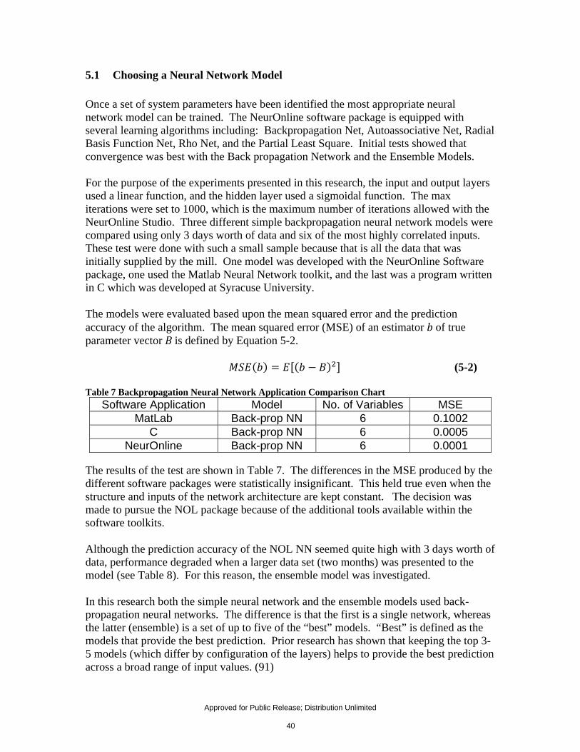
5.1 Choosing a Neural Network Model Once a set of system parameters have been identified the most appropriate neural network model can be trained. The NeurOnline software package is equipped with several learning algorithms including: Backpropagation Net, Autoassociative Net, Radial Basis Function Net, Rho Net, and the Partial Least Square. Initial tests showed that convergence was best with the Back propagation Network and the Ensemble Models. For the purpose of the experiments presented in this research, the input and output layers used a linear function, and the hidden layer used a sigmoidal function. The max iterations were set to 1000, which is the maximum number of iterations allowed with the NeurOnline Studio. Three different simple backpropagation neural network models were compared using only 3 days worth of data and six of the most highly correlated inputs. These test were done with such a small sample because that is all the data that was initially supplied by the mill. One model was developed with the NeurOnline Software package, one used the Matlab Neural Network toolkit, and the last was a program written in C which was developed at Syracuse University. The models were evaluated based upon the mean squared error and the prediction accuracy of the algorithm. The mean squared error (MSE) of an estimator b of true parameter vector B is defined by Equation 5-2.

(5-2) Table 7 Backpropagation Neural Network Application Comparison Chart

Software Application Model No. of Variables MSE MatLab Back-prop NN 6 0.1002

C Back-prop NN 6 0.0005 NeurOnline Back-prop NN 6 0.0001

The results of the test are shown in Table 7. The differences in the MSE produced by the different software packages were statistically insignificant. This held true even when the structure and inputs of the network architecture are kept constant. The decision was made to pursue the NOL package because of the additional tools available within the software toolkits. Although the prediction accuracy of the NOL NN seemed quite high with 3 days worth of data, performance degraded when a larger data set (two months) was presented to the model (see Table 8). For this reason, the ensemble model was investigated. In this research both the simple neural network and the ensemble models used back-propagation neural networks. The difference is that the first is a single network, whereas the latter (ensemble) is a set of up to five of the “best” models. “Best” is defined as the models that provide the best prediction. Prior research has shown that keeping the top 3-5 models (which differ by configuration of the layers) helps to provide the best prediction across a broad range of input values. (91)


The basic backpropagation (BPN) algorithm learns by adjusting the weights in the direction of the negative gradient of the performance function. The learning rate is a parameter that determines how much the neural network can change in each learning stage. In this application, the learning rate is multiplied times the negative of the gradient to determine the changes to the weights. The larger the learning rate, the bigger the step. The internal architecture of the BPN must be specified. The number of nodes in the first layer and the number of input variables must be the same. The number of nodes in the last layer and the number of output variables must also be the same. The hidden or intermediate layers (layers between the first and last layers) can be any size. The NeurOnline software can have up to three hidden layers, for a total of up to five layers. In general, a network has one hidden layer. The number of nodes depends on the complexity of the function that the network has to model, the more complex the function, the more nodes needed. The user can choose whether a layer uses the sigmoidal or linear function for its nodes. Once the architecture is specified, the BPN network can be trained and evaluated. The top five models together constitute the ensemble model. The comparison of the simple and the ensemble model is discussed below. The trials which considered a much larger data set more accurately represented the process. Two months worth of data was evaluated from the Plant Information System. The model was trained on data from 01 Jun 08 to 30 June 08 and was validated with data from 01 July 08 to 31 July 08. Table 8 demonstrates how the ensemble model outperforms the simple backpropagation algorithm when considering larger data sets. The algorithm tends to be more robust. If, for a particular input, one of the models makes a poor prediction, the ensemble model selection process will make sure the poor prediction is not allowed to inordinately influence the final result. Table 8 Comparison of Backpropagation Network to the Ensemble Model Algorithm Vectors MSE

Backpropagation 488 0.001

Backpropagation 17566 0.339

Ensemble 488 0.124

Ensemble 17566 0.125

Improvements to the ensemble model were made simply by filtering some of the outliers in the input. The same ensemble model described above (17,566 vectors) was reevaluated after removing outliers and anomalies. The performance of the model improved from a MSE of 0.125 to 0.018.


Figure 11 Neural network prediction results with no filtering of the data

Figure 12Neural Network improved just by filtering outliers in the data

The charts above show a plot of predicted versus actual fit, for the output variable. Although these results appeared promising, there was still room for improvements to make this information more helpful to the mill. After the model had been trained and evaluated, sensitivities analysis was useful for obtaining a better understanding with respect to the correlations in the data set. Sensitivity analyses also lead to a better understanding of the physical causality of the process. It helped identify inputs that had a strong influence on an output variable, or inputs that had little or no influence on the output.

Couch Vacuum Actual vs Predicted Values

-1

4

9

14

19

24

29

-1 4 9 14 19 24 29

Actual

Pred

icte

d


151617

1819202122

232425

15 17 19 21 23 25

Actual

Pred

icte

d


5.2 Sensitivity Analysis The NeurOn-Line application has the sensitivity analysis built into the neural network package. Sensitivities are derived from averages of local derivative information; mathematicians term this process as calculating derivates through finite differencing. Sensitivities in this system are defined and calculated as follows:

1. Select a random data point from the data series. 2. Generate the outputs for the data point using the model. 3. Perturb the jth input by a small amount, and recalculate the output. 4. For each output, form the ratio Sij = (output i' - output i)/(input j' - input j), where

the prime indicates the perturbed input and output. This is the estimate of the local derivative at the selected data point.

5. Repeat from step 3, for each input. 6. Repeat for another random data point.

The sensitivity value of output i with respect to input j is then calculated by taking the average of the Sij values, over the sample of randomly-selected data points. To calculate absolute sensitivities, the absolute values of Sij are averaged. Finally, each sensitivity is normalized by dividing the sensitivity by the standard deviation of the respective input variable. Without normalization, it would be impossible to compare sensitivities with respect to different inputs, because the sensitivities would have different units. With normalization, the sensitivities have the same units, specifically, the units of the output variable. For example, one sensor measurement in this research is feet per second and it needs to be compared to pounds per square inch. The sensitivity analysis shown in Figure 12 is for the top 5 variables that were selected as being most highly correlated to the predicted value. The five highest correlated variables included: the secondary refiner accept recirculation line, the disc thickener, the primary course screen accept flow line, the primary course screen consistency value, and the couch vacuum. The results in Figure 12 included prior time steps of the couch vacuum, which proved to be the most highly correlated of all the predictive inputs. However, the correlation tools allow investigators to eliminate this highly correlated value which may bias the prediction when sudden changes occur further upstream in the process. It was important to evaluate different models to measure the performance of the prediction and to identify areas where improvements can be made to make the model more useful for the paper mill analyst.


Figure 13 The results from the sensitivity analysis shows that the five highest correlated variables included: the secondary refiner accept recirculation line, the disc thickener, the primary course screen accept flow line, the primary course screen consistency value, and the couch vacuum.

. Figure 13 shows what happens when the couch vacuum prior values are removed as an input to the neural network:

Figure 14 Predictive performance is degraded when the output as a predictor is removed from the inputs.

The results above do not show as linear of a relationship between the actual and predicted values as was seen in Figure 11. The performance of the prediction degraded. With

Couch Vacuum Actual Value vs Predicted Value

1516171819202122232425

15 17 19 21 23 25

Actual Value

Pred

icte

d Va

lue


preprocessing of the data, however, this prediction can be improved. Since the grade of paper being produced is known to the operators at any point in time, it is fair to use this information and separate the data into basis weight grades. The following chart shows the improvement that can be gained by separating out a data regime (23 lb basis weight paper grade), and removing paper machine downtime.

Figure 15 When data regimes are separated and considered separately the neural network performance improves.

5.3 Optimizing the Neural Network Model When the 23lb basis weight grade was considered in isolation, a substantial improvement was realized. The MSE decreased from 1.13 to 0.125. Another interesting result from the sensitivity analysis and the correlation analysis was the high correlation of the secondary refiner accepts recirculation line. According to the engineers at the mill, the secondary refiner accepts recirculation line and the consistency of the "Stock to Fan Pump" sensor were closely related. At the recommendation of the mill engineer, the consistency output, a variable labeled “Stock to Fan Pump”, was evaluated as an input to the neural network. If the consistency meter was not picking up the fines (smaller particles) and it was producing an inaccurate reading, the system would try to compensate by sending more dilution water to this location. It would explain why this parameter would be so highly correlated with the variability in the amount of water being removed at the couch vacuum section on the paper machine. The spearman's correlation analysis showed the correlation of the consistency meter to be pretty close to the correlation of the secondary refiner recirculation line (24.02 vs. 23.51). Due to the high correlation, the stock to fan pump was evaluated as a sole input to the NN model, along with the two other most highly correlated variables.


151617

1819202122

232425

15 17 19 21 23 25

Actual

Pred

icte

d


Table 9 Comparison of Network Results with Single Variable Inputs Tested Variable MSE

Disc Thickener 0.166

Sec Ref Accepts 0.146

Stock to fan pump 0.088

The neural network model with the single input "stock to fan pump" had a low MSE, 0.088, which corresponds to high prediction accuracy with a single network input variable. These results show how much of an influence the “Stock to Fan Pump” had over what was happening on the paper machine. As previously noted, an inaccurate reading in this location would cause the system to overcompensate by adding too much dilution water. This would then cause swings in the amount of dilution water added to the system, and therefore affect the variability in moisture on the paper web. The NN model and the sensitivity analysis that followed helped the plant engineers to identify a correctable source of variability. To properly correct the problem, the mill would have to change the consistency meter from the flap type to an x-ray type sensor. While this research has proven this correlation, it is up to the mill as to whether it would be cost effective to make such a change.

5.4 Conclusions Complex systems, like the one found in this industrial process, require a complex design process when developing a predictive model. In this research, it was apparent that the variable “Stock to Fan Pump”, which measured the stock consistency, had a significant correlation to the sensor readings on the couch vacuum. Although the mill was aware of some of the correlations that existed in the process, it was the combination of a preliminary correlation analysis, a proper neural network model, and a follow up sensitivity analysis that helped to pin point the precise source of process variability. Careful consideration of the problem domain is imperative when selecting the best model and it may be necessary to revisit the model at any given step in the design process. As shown in this research, once an initial iteration of feature and model selection has occurred, more information about the problem domain becomes apparent. It may be necessary to look more closely into a specific set of sensors or process nodes to further investigate if more features or sensory information, which may have been previously overlooked, produces a more accurate model. Investigating extremely large sensory systems with many data collection points can be tedious and complex, but a methodical process can help to improve prediction accuracy.


The next Chapter will look at models which can predict when paper machine downtimes, or failures, will occur. In trying to predict failures, finding variables that are highly correlated to paper machine paper breaks is more challenging than the problem of predicting the output of couch vacuum to identify the sources of variability.


6 PATTERN MATCHING TOOLS FOR EVENT PREDICTION

6.1 Background Another operational problem of interest is in predicting when a paper machine break will occur. This classic “fault detection problem” has been explored in other works which were presented in the background section. Some of the approaches presented in the background section inspired the research explored here. The problem of detecting paper machine breaks is far less constrained than the problem of identifying sources of variability affecting the couch vacuum because there are many more outside factors which may contribute to a PM break than there are factors influencing variability in the moisture on the sheet. Some breaks were due to unforeseen mechanical failures, some from contaminants on the sheet (excessive dirt or oil), some were due to variations in the moisture on the sheet which caused differences in the stress and strain imposed in the cross-direction and machine direction of the sheet, some were scheduled maintenance downtimes, and some were due to outside factors that were completely unforeseen and unpredictable. Most prediction algorithms are limited in being able to predict failures in such environments because the algorithm tends to look for linear correlations. In the case of the PM breaks on a machine that runs several different grades of paper, there is not one correlation to be found. Instead there are subsets of correlations which may or may not emerge with more complicated models. The NeurOnline software package discussed in the previous chapter had many limitations in dealing with this problem. One limitation was that NeurOnline was designed to deal with continuous input and output values. The status of the paper machine was discrete. After preprocessing the data, there was a class of running records and a class of records that represented the conditions of the process just prior to a break occurring on the machine which is referred to as “fault indicating” records. Another reason for the challenge in using the NeurOnline prediction tools for fault detection is that the classes of good and bad operating modes were extremely disproportionate. There were a total of 96670 records; 95125 of these records were records that were representing a normal mode of operation, but only 1545 records were records that represented the fault indicator records. This corresponds to 309 paper machine breaks in one year. Although it is good for the mill that there were significantly less times the paper machine was down then running in a mode of good operation, this meant that the data set was very heavily weighted toward the running class. Having a significant amount of data in one class, and very little in the other, makes it very difficult to develop predictive models. To illustrate this point, consider having 60 red balls in a bag and one blue ball. It is very easy for one to predict that a ball selected at random from the bag will be a red ball, and the overall prediction accuracy would be around 98%. To further complicate the problem, the times when the paper machine was not running needed to be removed from the data set, and adjustments needed to be made for lag times.


During paper machine downtimes, some sensor readings become erratic. It was the period of time, 5 time steps just prior to a break, which were considered the most important. This corresponded to 25 minutes prior to a paper machine break. In section 4.2 the challenge of establishing ground truth in the data was discussed. Resolving discrepancies between the operator logs and the paper machine sensor readings was challenging. To evaluate each models performance, the number of faults detected was recorded as well as the number of correctly classified running vectors. The following equations were used to assess the prediction accuracy of each model:

%

(6-1)

%

(6-2)

%

(6-3)

%

(6-4)

The % predicted running can be calculated as 1- % false alarm. The % missed failure can be calculated by 1- %failure detection. So a low false alarm rate means that a high number of running vectors were classified correctly, and high % failure detection means that a high number of fault indicating vectors were classified correctly. In an operational setting the mill would use this information to alert the operators when a paper machine break is likely to occur. For each model described in this chapter, results are reported for the L1 and L2 distance measures, all grades lumped together (not normalized) (no separation of basis weights) , and all grades normalized, and the 23lb basis weight normalized and the 23 lb basis weight not normalized. The 23 lb basis weight is the most commonly produced grade on Paper Machine 3 (PM3). Occasionally three other higher basis weight grades are produced, but breaks are not as common with the higher basis weight grades. It would be recommended, however, that before implanting these techniques into an actual mill setting, each grade should be evaluated. It is fair to assume in an operational setting that the system could store a separate model for each grade of paper produced on the paper machine. Another point of consideration is that major process changes will require retraining of the models. For this study, the production rate was reduced significantly in 2009, so 2009 was not used for this study. If implemented in this mill, the models would need to be retrained at the lower production rate.


6.2 Data Preprocessing The data preprocessing and feature selection process was done differently than in the previous chapter. A conventional analysis to find a linear mapping of correlated variables would have tried to fit the many modes of operation into a single input-output mapping. This did not seem to be the best solution. The feature selection process was evaluated using the Tukey Test (t-test). The Tukey Test is a simple statistical test that can be used to which find which features vary the most between the two classes. The basic algorithm is as follows: (83) 1. Located the largest and smallest of the overall population 2. If both the largest and smallest value occurs in the same sample, we cannot conclude that the means of the two populations are different. 3. Locate the largest and smallest values in sample 1. 4. Locate the largest and smallest values in sample 2. 5. Consider the sample containing the smallest value in the two samples combined, as found in Step1. Count the number of values in this sample that are smaller than the smallest value in the other sample. 6. Consider the sample containing the largest value in the two samples combined, as found in Step 1. Count the number of values in this sample that are larger than the largest value in the other sample. 7. The sum of the counts obtained in Step 5 and 6 is the numerical value of the test statistic T. The original data set, which contained 54 variables, was reduced based upon the highest ranking t-test variables and the highest differences in the means between the two classes. The first five variables that resulted from the t-test are shown in Table 10. Table 10 T-Test Highest Values indicate the variables with most class differentiation Highest T Test Values T-Test S3_33CC356PV PriCrs Feed Consistency 6 S3_33LC907_PV Blend Chest Process Value 5 S3_33LC907A_PV BLEND CHEST 5 S3_43PC455_PV 3rd DRYER SECTION 24 S3D_WIRE_TURNING_SACT 47

The second set of variables to be included was calculated by taking the mean of the population from each class. The variables with the largest difference between the means were selected.


Table 11 Variables with largest difference in mean between two classes Largest Difference in Mean Values S3_33CC216_PV STOCK TO STUFF BOX S3_33LC161_PV DISK THICKNER S3_43PC371_PV COUCH S3_33CC201_PV STOCK TO PRIMARY REFINER S3_33PC515_PV PRI COARSE SCREEN FEED

The primary course screen feed consistency (S3_33CC356PV) and process value of the flow of the stock to the screen itself (S3_33PC515_PV) were eliminated because they were so far back in the process that is extremely difficult to determine an accurate lag. This was especially true considering the fact that an agitated HD storage tank exists between the screens and the paper machines to provide a varying 60 minute buffer in the process. Also, the mills confidence in the accuracy of the consistency sensor was low.

6.3 Mean Vector Distance There are some commercially available software packages that quantify a vector of the “mean” operating conditions when running in a good operating mode. These software packages tend to focus on specific control loops, or limited regions of the industrial processes (screening system, for example). When the process starts to deviate from the “mean”, the operator is alerted. The success of these packages will depend on how often the mill makes process changes, grade changes, and how much inherent variability is present in the process. Initially, this research looked to characterize mean vectors for each grade as other commercially available software packages have done. The training set was loaded and broken up into grades. The mean vector for each grade was computed for the case of running and for the case for the fault indicating records. When an unknown vector was presented to the system, the L1 and L2 distances were evaluated to see if the unknown vector was closer to the mean vectors of the going down case or the running case. The mean vectors for each grade were used to predict the unknown vector. The pseudo code is shown below:

1) Load training data from the mill data file based on some time window. 2) Load testing data from the mill data file for the subsequent time window. 3) Create a bin of data records for each type of grade/status that exists. 4) For every bin, create a vector that represents the mean of each attribute of the

vectors in that bin. This is mean vector for that grade/status. 5) For each vector in the test data, find the closest mean vector from step 4, use that

to predict status of the test vector as a running or going down vector. 6) Validate with the actual status and report the results. 7)


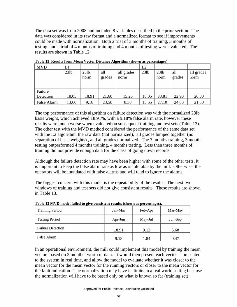
The data set was from 2008 and included 8 variables described in the prior section. The data was considered in its raw format and a normalized format to see if improvements could be made with normalization. Both a trial of 3 months of training, 3 months of testing, and a trial of 4 months of training and 4 months of testing were evaluated. The results are shown in Table 12. Table 12 Results from Mean Vector Distance Algorithm (shown as percentages) MVD L1 L2

23lb 23lb norm

all grades

all grades norm

23lb 23lb norm

all grades

all grades norm

Failure Detection 18.05 18.91 21.60 15.20 18.05 33.81 22.90 26.00 False Alarm 13.60 9.18 23.50 8.30 13.65 27.10 24.80 21.50

The top performance of this algorithm on failure detection was with the normalized 23lb basis weight, which achieved 18.91%, with a 9.18% false alarm rate, however these results were much worse when evaluated on subsequent training and test sets (Table 13). The other test with the MVD method considered the performance of the same data set with the L2 algorithm, the raw data (not normalized), all grades lumped together (no separation of basis weights) , and all grades normalized. The 3 months training, 3 months testing outperformed 4 months training, 4 months testing. Less than three months of training did not provide enough data for the class of going down records. Although the failure detection rate may have been higher with some of the other tests, it is important to keep the false alarm rate as low as is tolerable by the mill. Otherwise, the operators will be inundated with false alarms and will tend to ignore the alarms. The biggest concern with this model is the repeatability of the results. The next two windows of training and test sets did not give consistent results. These results are shown in Table 13. Table 13 MVD model failed to give consistent results (shown as percentages).

Training Period Jan-Mar Feb-Apr Mar-May

Testing Period Apr-Jun May-Jul Jun-Sep

Failure Detection 18.91 9.12 5.68 False Alarm 9.18 1.84 0.47

In an operational environment, the mill could implement this model by training the mean vectors based on 3 months’ worth of data. It would then present each vector is presented to the system in real time, and allow the model to evaluate whether it was closer to the mean vector for the mean vector for the running vectors or closer to the mean vector for the fault indication. The normalization may have its limits in a real world setting because the normalization will have to be based only on what is known so far (training set).


The next three months worth of data may fall out of the bounds of the normalization determined on the training set. If it this model is implemented, the mill should renormalize the data each time it trains a new model. If the mill would prefer to use raw data with this method, the top performance was 18.91% failure detection with a false alarm rate of 9.18%, but this was not repeatable in subsequent months. When the normalized data was considered L1 tended to outperform L2. When the nonnormalized data, was considered, the L2, or Euclidean Distance, measure outperformed the L1, city walk, distance measure. The results from the mean vector distance model indicated that having a single mean vector for the case of good running vectors for each grade, and one mean vector for the case of fault indicating vectors for each grade could give reasonable results that would have added cost benefit to the mill. However because of the variability in the process, a single mean vector did not prove to give repeatable results. This model also does not allow the flexibility necessary to allow the mill to reduce the false alarm rate, or increase the false alarm rate in times when a more expensive grade is being produced. Another limitation of this model is that it can be limited when detecting paper machine failures where there are many modes of good running conditions, and many different reasons why a failure may occur. The feature vectors may be labeled as being “good running vectors” or “failure indicator vectors”, but within these two classes, there may be many regions of good and poor operating modes. The benefits of using both K-Nearest Neighbor and modifications to the K-Means clustering models, which will find multiple means in each class, will be explored in the next sections.

6.4 K-Nearest Neighbor K- Nearest Neighbor (KNN) is used to find the nearest neighbor that has the least distance to an unknown vector. (92)Both the L1 and the L2 distance measure was used to measure the distance of an unknown vector in the test set to the closest vector in the training set. If the closest vector from the test set was a running vector, than the prediction of the unknown vector was running. If the closest vector from the test set was a fault indicating record than the unknown vector was classified as a fault indicating vector. Using this rather simple technique the prediction results reported in Table 14 were achieved.


Table 14 Comparison of performance of L1, L2 distance functions and data sets on KNN (shown as percentages).

KNN L1 L2

23lb 23lb norm

all grades

all grades norm

23lb 23lb norm

all grades

all grades norm


The best performance was achieved with the 23lb normalized data set using the L1 distance measure. The failure detection was 6.59% with a 3.17% false alarm. This model would be useful for a mill that was looking for a 5% reduction in paper machine breaks with less than 3% false alarm. The general algorithm for K-Nearest Neighbor is described below:

1) Load training data from the mill data file based on some time window. 2) Load testing data from the mill data file of a subsequent time window. 3) Separate the testing records into bins of running and going down records. 4) Compare the L2 distance of each of the test records against each of the training

records 5) Find training record that is of minimum distance to the test record in question. 6) Compare the status of each test record with the training record that was found to

be closest to said test record. 7) Summarize the number of times that the nearest training record and the test

record were of the same or different status and report the results

6.5 Modified K-Means Algorithm The modified k-means algorithm was a hybrid of both an unsupervised and supervised learning system. The unsupervised method of clustering allows clusters to emerge within the classes. These clusters may be thought of as groups of patterns whose members are more similar to each other than to the other patterns- or of major departures from expected characteristics. Properly representing these clusters is essential to characterizing the current state of the system. It is a supervised learning system, because the vectors are labeled as fault-indicating vectors and vectors representing good running conditions. There are many reasons for the emergence of subclasses within the two main classes. There are four different grades of paper that are produced on this machine, each with its own optimum settings for most effective operation. There are variations on individual fiber strength of the incoming raw material, variations on debris load, process variations


like poor refining, screening, or instrumentation/ control loop changes and many different ways the equipment or operators will respond to these changes. The algorithm presented finds clusters of multidimensional points which describe the process states. The algorithm was modified as described in the following sections.

6.5.1 Modifications to the Java ML Toolkit An open-source machine learning library called Java -Machine Learning (Java-ML) (http://java-ml.sourceforge.net/) was used to provide the algorithm for performing the K-Means clustering algorithm on the mill data. (93) The version used for this work is 0.1.4. Java-ML provides an extensive number of machine learning algorithms, of which K-Means is one. The algorithms described in the next sections call the basic K-means algorithm that came with this package. Appendix A includes modifications described in this section alone that were required to make the library itself more user-friendly. The Java-ML provides a straight forward and uniform mechanism for providing user data to its algorithms. (94) Minimal effort was required to modify existing mill data to translate the data into the Java-ML format. Every record in the Java-ML library is represented as an “Instance”. Instances can be of arbitrary length and every value within an Instance is an “Attribute”. Instances can be grouped into collections known as “Datasets”. These Datasets can represent raw data from a file or, as with the K-Means algorithm, the instances that fall within a given cluster. Several modifications to the Java-ML library where necessary. Since the library was open source, it was possible to make a copy of the source code and effect the necessary modifications. The K-Means clustering algorithm was copied into the code base and renamed “MyKMeans” in order to not conflict with the java-ml namespace. Then great care was taken to split the cluster method into the calculation of the cluster centroids and the binning of the input data into the appropriate clusters. The reason for providing this separation was two-fold. First, the original code did not allow easy access to the centroids without redoing the entire reassignment of all vectors to their corresponding cluster. There were times when only the cluster centroids were needed. Allowing the researcher to make the call to only perform these calculations without the computational and storage overhead of binning the data into clusters sped up the run times for experiments and allowed running the calculations on larger sets of data. The second, and probably more important, reason for doing this was so that access to the calculated centroids could be obtained. This was beneficial for runs where a training set was used to generate the cluster centroids and then another test set was binned into those centroids to test the efficacy of the K-Means clustering algorithm with respect to downtime prediction. For these types of experiments, it was totally unnecessary to generate the bins for the training data, and splitting the cluster method into pieces allowed for a calculation of cluster centroids with one set of data (training data) and a binning of another set (test data).


http://java-ml.sourceforge.net/

The original K-Means algorithm in the Java-ml library lacked the ability to access the calculated centroids, so an accessor method was added to provide access. The library also had documentation indicating that it was possible to utilize a user-provided random number generator, but this was not the case. The library only provided a random number generator initialized with the system clock, making repeatable results impossible. So constructor for creating a MyKMeans instance were added to allow the user to initialized the algorithm with either a pre-constructed random number generator or a long seed value. Another problem with the Java-ML library was the average function within the DatasetTools class calculates a mid-range average and not an arithmetic mean. This caused some consternation when comparing results from the java code against trails evaluated in Excel. Once the disparity was found, a new average method that calculates the arithmetic mean for Instances was implemented external to the Java-ML library. Unfortunately, the Java-ML library’s documentation of the “average” method was not specific about its implementation.

6.5.2 Cluster Evaluation One of the biggest criticisms of the K-Means algorithm is that the user needs to specify the number of clusters up front. It's rarely obvious as to how many clusters is necessary, even as a starting point. One way to overcome this limitation is with a cluster evaluator. The cluster evaluator identifies how many clusters are needed by identifying the number of clusters in which the inter-cluster to intra-cluster distance has reached a minimum. This method of cluster evaluation was presented in a work by Ray and Turi in 1999 (95). There are several other methods of cluster evaluation available in the JavaML library but this method was recommended by an expert in the field of machine learning. This procedure iteratively tries out different values of K and selects the one with the highest dissimilarity ratio. The dissimilarity ratio measures the dispersion of the different clusters. The number of clusters needed depends highly on the nature of the data. The basic algorithm is described below.


1) User specifies the time interval of records to use for the evaluation as well as the starting k and ending k to evaluate.

2) From the starting k to the ending k, generate clusters of going down and running records for that k.

3) For each of those cluster sets, calculate the intra-cluster distance by summing the distances of every vector with its cluster and divide the sum of all vectors in all clusters by the total number of vectors to get the average intra-cluster distance.

4) For each cluster centroid, calculate the distance to each of the other clusters in the cluster set, taking the minimum distance calculated. Sum these min distances and use this as the inter-cluster distance.

5) Divide the intra-cluster distance by the inter-cluster distance to get the score for this value of K.

The cluster evaluator evaluated the clusters that were formed for the fault indicating records and for the running records independently. The basic equation for calculating the compactness of clusters is described in the following equations.

(6-5)

∑ ,

| |

∑min ,1, 2, … , 1; 1, … ,

(6-6)

The results from the cluster evaluator are shown in Figure 15. The compactness of the clusters tends to level out around 10 clusters, so this was the initial cluster value that was used in the following approaches. Tests were conducted to evaluate the performance of more clusters, but the best performance across all models was achieved with an initialization of 10 clusters. Some models converged on a model that was less than 10 clusters, depending on the nature of the data. This will be explained further in the next sections.

Figure 16 Cluster Evaluator for 6 months of data shows that 10 clusters should be the initial value for K.


6.5.3 Semi-Fuzzy K-Means The fuzzy k-means method clustered the good running records and the fault indicating records simultaneously and defined a probability of membership into both. This method is different from KNN in that it considers the unknown vectors position relative to a mean centroid which characterized a subset of fault indicating records and good running records. Fuzzy membership into a set or cluster in this case, is based on the degree of membership that some element may have of belonging to that set. (96) Initially, the algorithm looked at the probability of membership into all clusters, which would have been a truly fuzzy system. However, this method did not give meaningful results, so a modified approach was used. Instead of looking at all clusters, the evaluation of each unknown vector was determined by its position to the two closest clusters. If the closest cluster belonged to the set of fault indicating clusters, then the unknown record was classified as failure detection, if the closest cluster belonged to the set of good running vectors, then the unknown record was classified as a good running vector. If the unknown vector fell someplace half way between a good running cluster and fault indicating cluster, then the vector was labeled as 50/50 failure detection for vectors that should have been classified as failure detection, and 50/50 false alarm for vectors that should have been classified as good running vectors. In the operational setting, the failure detection would signal a high alarm, the 50/50 detection would be a low alarm. To use this tool, the analyst would: load a data set, specify the training year, training month, number of months to train, the number of initial clusters, and a threshold of how many vectors are needed to make a strong cluster. The default on this value would be 15 for 3 month training, 3 month testing evaluation. Since each paper machine break had 5 vectors associated with it, 15 vectors were considered the minimum to create superior clusters. The analyst then loads the data, and trains the model. Figure 16 shows what a trained model would look like. An important thing to note is that despite the fact that the initial number of clusters specified to the k-means algorithm was 10, there may be far fewer clusters in the trained model because the cluster did not have the minimum number of vectors required.


The Graphical User Interface (GUI) for this method is shown in Figure 16.

Figure 17 Fuzzy K-Means GUI displays specified clusters and cluster sizes For research purposes, the analyst will then load the test set. Preliminary experiments showed that this test set should be the subsequent months following training and should not exceed the training period. In a mill setting, the system would read in each vector at a given time stamp and evaluate whether the record would be classified as a good running vector or a vector that was indicative a paper machine break occurring (positive failure detection) or a low alarm would signal which would indicate that the unknown vector was somewhere in the middle of a good cluster and a fault indicating cluster. The results are shown in Table 15. Table 15 Comparison of performance of L1, L2 distance functions and data sets on Semi-Fuzzy K-Means (shown as percentages) Semi-Fuzzy K-Means L1 L2

23lb 23lb norm

all grades

all grades norm

23lb 23lb norm

all grades

all grades norm

Failure Detection 44.41 91.12 24.94 44.73 62.18 13.18 24.94 57.33False Alarm 22.18 79.76 26.81 17.45 51.60 30.26 23.35 37.8950/50 Failure Detection 12.32 2.87 7.97 23.39 7.16 23.78 5.66 28.0250/50 False Alarm 19.14 10.54 3.68 34.47 14.60 41.14 6.72 24.42


The best performance of this algorithm was achieved with the normalized data set which included all grades and an L1 distance measure. The performance was 44.73% failure detection with a 17.45% false alarm rate. Table 16 shows the repeatability of results with this model. Table 16 Comparison of performance of Semi-Fuzzy K-Means over subsequent train/testing sets (shown as percentages).



Failure Detection 44.73 73.67 23.42

False Alarm 17.45 37.51 8.53

50/50 Failure Detection 23.39

15.38 17.89

50/50 False Alarm 34.47 43.57 14.51 Table 16 demonstrates that this model is not very consistent in its performance; however it consistently detected a high percentage of paper machine breaks. Also the % failure detection is consistently much higher than the false alarm rate. The other benefit of this system is that a graduate alert system could be implemented. An example of how this might work is shown in Table 17. Table 17 Example of implementation of the semi-fuzzy k-means model Time Prediction Status

8/20/2008 7:10 running good 8/20/2008 7:15 50/50 fault low alert 8/20/2008 7:20 50/50 fault low alert 8/20/2008 7:25 approaching failure high alert 8/20/2008 7:30 approaching failure high alert 8/20/2008 7:35 approaching failure high alert


The general algorithm is described below: 1) Load training data from the mill data file based on some time window, number of

clusters (k), and minimum members per cluster. 2) Load testing data from the mill data file based on another time window, and the

number of clusters contributing to the prediction of system status. 3) Generate cluster sets from the doing down and running records. This will give

two cluster sets each comprised of k clusters. 4) Remove any clusters not containing a minimum number of vectors as specified by

the user. 5) Load test data. 6) For each record of the testing data, calculate the distance to all the centroids of

all the clusters in both cluster sets. 7) Order the results from closest to farthest distance. 8) Use the number of the two closest clusters and the distances of each to determine

how much each cluster contributes to the prediction of system status. 9) Validate against known status to evaluate the prediction accuracy of the model.


6.5.4 Quality Threshold K-Means The quality threshold k-means (QT K-Means) algorithm was a more favorable approach for many reasons. Quality of the clusters are ensured by finding clusters whose diameter does not exceed a given user-defined diameter threshold. This method reduces the number of dissimilar samples from being forced under the same cluster and ensures that only good quality clusters will be formed. Two quality threshold implementations were explored. In the first model, the “quality clusters” were made up of fault indicating vectors alone. The objectives in forming the clusters were to maximize the number of fault indicating records (fault detection) in the cluster, while minimizing the number of good running vectors in the cluster (false alarms). The vectors that fell outside the bounds of the clusters were then considered to represent a good operating condition, while the vectors that fell within the clusters were considered fault indicators. In the second model, the “quality clusters” were made up of the good running vectors. The objective here was to minimize the number of vectors that fell within the cluster boundary that were fault -indicating vectors, while simultaneously maximizing the number of vectors that were good running vectors. Due to the amount of process variability and seasonal changes that occur in the mill setting, these objectives are set after each training period, by the analyst, using the GUI developed for this system. The threshold values are determined from the training records as will be discussed. The general algorithm for the QT K-Means algorithm is described below:

1) The user loads the operator log and the mill data file specifying the training data set.

2) Clusters are formed from the training data set. Clusters can be based on going down records or running records, depending on user preference.

3) For each cluster, the threshold (percent of members in the cluster used to calculate the outer bound of the cluster) can be set by the user.

4) The user then specifies the testing data set, at which point the running and down records will be inserted into the most appropriate cluster.

5) The distances from the cluster centroid to each of the test records is calculated and compared to the outer bound given by the threshold.

6) If the record falls outside cluster bounds it is considered outside of the class that makes up the clusters, and it is classified accordingly.

6.5.4.1 QT K-Means Model One (QTM1) A small subset of data was plotted in Figure 17 to illustrate the first model. The red squares are fault indicating records and the blue diamonds are good running records. Although the number of good running records far outweighs the number of fault indicating records, an equal number of each class is depicted in the chart in Figure 17 for illustrative purposes. In reality, there would be far more blue diamonds than red squares on this chart.


Figure 18 When implementing QT K-Means Model One clusters are formed around the fault indicating records. The size of the cluster is adjusted by changing the threshold value.

As previously noted, once clusters of going down records are formed from the training set, the threshold values are manually adjusted to minimize the number of running records that are classified as down records, and to maximize the number of fault indication records that are classified as running records. This means that the distance surrounding each cluster is adjusted. This value can be adjusted by the analyst depending on the acceptable false alarm rate. If the mill is running higher cost product, for example, and they want the system to be more sensitive and to alert the operators more often when a paper machine break may occur, the analyst or the engineers would increase the sensitivity of the system. A graphical user interface (GUI) was developed to implement this algorithm. A screen shot of this GUI is shown in Figure 18.


Figure 19 GUI for QT-K-Means model one shows how the threshold values of each cluster can be adjusted in the training set to improve prediction accuracy. The implementation of this model requires some analyst training as it is currently designed. The training set is read in and the clusters are formed. The analyst would then adjust the threshold values of each cluster in order to maximize the number of fault indicating records (fault detection) in the cluster, while minimizing the number of good running vectors in the cluster (false alarms). One benefit of this model is its ability to allow the analyst to see what events are making up each cluster. In order to understand what information the various clusters represented, the events from the operator logs were mapped to the clusters which were defined by fault indicator vectors. Each single event has 5 corresponding vectors associated with it because 5 time steps prior to a break occurring were labeled as fault indicating vectors. It is interesting to note that the 5 vectors associated with a single event do not necessarily get clustered together. This is due to the fact that the various different causes for paper machine breaks may occur at various time steps. For example, a vector 25 minutes back in the process may be imposing noise into the system because it actually represents a mode of normal running conditions and the circumstances which may have caused the paper machine break to occur may not have manifested themselves at this point in time. Nonetheless, assumptions needed to be made to try to capture the information leading to a paper machine break in a consistent manner. Five time steps seemed to be a reasonable assumption. The overall prediction results for this model are shown in Table 18.


Table 18 Comparison of performance of L1, L2 distance functions and data sets on Q-T K-means Model One (shown in percentages). QT-Model One L1 L2

23lb 23lb norm

all grades

all grades norm

23lb 23lb norm

all grades

all grades norm

Failure Detection 19.48 15.30 11.80 14.39 19.50 10.90 16.70 13.88False Alarm 13.69 12.65 12.10 11.30 12.90 12.00 17.10 11.95

Some examples of the types of events which were depicted by the fault indicating vectors are shown in Table 19. Originally, the mechanical, electrical failures, and outages were removed from the training set because they were considered to be catastrophic or unpredictable events. However, they were added back into the analysis because it is unclear, in some cases, whether changes in process conditions may have caused the failures to occur or if the operators may have done certain things just prior to an outage which would have been picked up by the model. Some events which are associated with the fault indicating vectors may be captured in clusters in the training set, but due to operational or equipment changes, they may sometimes disappear from the test set. In looking at the operator log, sometimes the electrical failures were not a result of something catastrophic, but rather they were a result of logic issues in the control loops. Logic issues in the control loops could very well be something that can be detected by the model. Another reason it seemed important to include them is because it is not always obvious from the operator logs that the operators were completely confident on the assessment of the cause of the break. Without these events included the prediction accuracy was lower for a couple of reasons. The first reason is because of the nature of the clustering algorithm itself. All fault indicating vectors have a membership into a cluster. If these vectors show up in the test set, and if they have no cluster that has been previously defined that fits their characteristics; they will be forced into another cluster. However, they would likely be far away from the centroid cluster and boundary separating the classes. This would result in a misclassification of that vector. Another thing to consider in the analysis of the results is the fact that the clusters need to have enough vectors to characterize a particular mode of operation; otherwise they could be representing outliers in the data. For example, in the table below clusters two and three were eliminated because they only had one vector which defined them and this is not statistically significant enough to be considered a strong cluster. A strong cluster was defined as having a least 15 vectors. The following results were based off a data set that included only the records for the 23 lb basis weight. It is fair to assume in an operational setting that the system could store a separate model for each grade of paper produced on the paper machine.


Table 19 the QT K-Means Model allows for the mapping of Operator Log to clusters Cluster Number

Break Event Type (No. Occurrences) Training Set

Break Event Type (No. Occurrences) Test Set

0 Hydrasizer (10) Trim Fold (2) Mechanical Failure Hydraulics (1) Mechanical Failure Gasket Seals (5) Other (7)

Mechanical Failure (5)

1 Hydrasizer (15) Missed Turn Up (MTU) (1) Other (25) External Failure Tri-Gen (5) Electrical Failure (2) Trim Fold (10) Clothing Worn Out (5) Break on Draw (1)

MTU (1) Other (20) Electrical Failure Drive (5) Misc Electrical Failure (5) Mechanical Failure (5) Stock Lump (5)

4 MTU (3) Other (15) Break due to Grade Change (5) Break on Draw(10) Scheduled Outage (5)

MTU(6) Other (41) Electrical Failure Drive (5) Electrical Failure Misc (5) Mechanical Failure (5) Trim Fold (9) Clean Up (5)

5 Hydrasizer (5) Other (11) Misc Electrical Failure (5) Misc Mechanical Failure (5) Trim Fold (8) Stock Lump (5) Slime (3) Unscheduled outage overrun (5)

Other (4) Mechanical Failure (5) Scheduled outage (1) Clothing (5)

6 Mechanical Failure Stock Prep (5) Other (5)

No events in test set

7 Hydrasizer (5) MTU(9) Other (10) Misc Electrical Failure (10) Trim-fold (9) Stock Lump (7) Break due to grade change (5)

Other (8) Electrical Failure (3) Mechanical Failure (2) Stock Lump (5) Clothing wore out (5)

8 Other (15)

MTU (8) Electrical Failure (7) Mechanical Failure (10) Other (32) Break on Draw (3)

9 Hydrasizer (9) MTU (6) Other (23) Mechanical Failure (3) Stock Lump (5) Clothing Worn Out (5)

Other (10) Electrical Failure (5) Clean Up (5) Clothing Worn Out (10) Outage Scheduled (4)

Another benefit of this model is that the performance of each cluster can also be considered in isolation. The overall performance of the system described above for the


training months of January -March, testing from April to June, with low sensitivity, was a break detection of 12.6% with a false alarm rate of 7.6%. A small increase in sensitivity improved the break detection to 19.5% with a false alarm rate of 12.9%. The breakdown per cluster is shown in Tables 20 and 21. Table 20 The breakdown of performance per cluster with low sensitivity

Cluster No. 0 1 2 3 4 5 6 7 8 9

Break Detection 0.00% 0.00% 0.00% 0.00% 28.40% 0.00% 0.00% 29.00% 0.00% 21.30% False Alarm 12.50% 4.60% 0.00% 0.00% 15.70% 9.20% 0.00% 11.70% 0.00% 7.70%

Table 21 The breakdown of performance per cluster when the sensitivity is increased Cluster No. 0 1 2 3 4 5 6 7 8 9

Break Detection 0.00% 26.00% 0.00% 0.00% 28.40% 27.30% 0.00% 35.40% 3.90% 21.30% False Alarm 12.50% 19.34% 0.00% 0.00% 16.10% 17.30% 0.00% 19.30% 1.90% 9.70%

The performance of this algorithm was then evaluated for repeatability of results. Table 22 shows the performance of the low sensitivity model using 3 months of training, 3 months of test data starting on January 1 2008. Table 24 shows the same model with a higher sensitivity. The total number of clusters used in this experiment was 10. The month shown in the column header was the start month of the three months of training, and the subsequent 3 months were used for testing. The threshold adjustment is done by the analyst prior to loading the validation set. The threshold values are adjusted to 0 for clusters with less than 15 vectors. Then adjustments are made to the threshold values to raise the number of training set running vectors that fall outside the threshold value enough to achieve about 80%prediction accuracy of the good running vectors per cluster without drastically compromising the number of fault indicating vectors that fall within the cluster threshold boundary. The reason for doing this is to minimize the number of false alarms. If the mill wants a more sensitive system, then they would be able to achieve this by allowing for more false alarms. The results in Table 22 show what the results would be if the mill decided to have a low sensitivity, or low false alarm rate.


Table 22 QTM1 gave repeatable results at low sensitivity values.




False Alarm 7.60 6.60 5.20

Table 23 Threshold values for low sensitivity QTM1 2008 23 lb Data Set - 8 Variables Threshold Values – low sensitivity Cluster 0 1 2 3 4 5 6 7 8 9 J--M 0.10 0.20 0.00 0.00 0.40 0.15 0.00 0.14 0.00 0.30 F-A 0.40 0.60 0.00 0.00 0.00 0.57 0.48 0.45 0.35 0.29 M-M 0.00 0.20 0.18 0.57 0.00 0.00 0.00 0.00 0.48 0.20 Improvements in the break detection can be realized if the mill is willing to accept a higher false alarm rate. Table x shows the break detection improvement with a less sensitive system. Table 24 QTM1 gave repeatable results at higher sensitivity values.




False Alarm 12.9 12.8 13.5

Table 25 Threshold values for high sensitivity QTM1 Changes in Threshold Values to Increase Sensitivity Cluster No. 0 1 2 3 4 5 6 7 8 9 Low Sensitivity 0.10 0.20 0.00 0.00 0.40 0.15 0.00 0.14 0.00 0.30 Increased Sensitivity 0.10 0.60 0.00 0.00 0.42 0.35 0.00 0.46 0.60 0.40

These tables above demonstrate the benefit of the Q-T K-Means algorithm. The mill is able to adjust the sensitivity of the system to a point that is tolerable and reasonable for the operators. They can adjust the threshold to a level in which the system offers a reasonable cost benefit without inundating the operators with false alarms. Also, the repeatability of results is best with this model


6.5.4.2 QT K-Means Model Two (QTM2) The second approach with the QT K-Means method involved clustering only the running vectors. The clusters were formed around the running vectors in a similar fashion to the first method. In this approach, however, the clusters of good running records are formed from the training set, the threshold values are manually adjusted to maximize the number of running records that are classified as running records, while also maximizing the number of fault indication records that are classified as fault indication records. As before, the distance surrounding each cluster is adjusted, and if the number of records which makes up a given cluster is smaller than five, then the cluster is eliminated. The results from the method of clustering the good running records alone have more statistical significance because of the fact that there are more vectors to make up the clusters of good running conditions. The results of this method are shown in Table 26. Table 26 Comparison of performance of L1, L2 distance functions and data sets on Q-T K-means Model Two QT-Model Two L1 L2

23lb 23lb norm

all grades

all grades norm

23lb 23lb norm

all grades

all grades norm


The best performance of this model was achieved with the L2 distance measure, 23lb basis weight data set with no normalization. Some of the benefits of this system include the fact that the sensitivity of the system is adjustable, and it achieves a low false alarm rate. One of the limitations of this model is that the failure detection is lower than some of the other models. Also, there is some operator/analyst training and experience that would be necessary to adjust the threshold/ sensitivities of the system.

6.6 Summary A summary of the results for the models presented in this chapter is shown in Table 27. The benefits and limitations of each algorithm are summarized in Table 28.


Table 27 Summary of results of Models Investigated Year 2008 Training Set Jan-Mar

Test Set April-June

L1 MVD KNN Fuzzy-K QT-K 1 QT-K2

23lb Failure Detect 18.05% 4.87% 44.41% 19.48% 4.93%False Alarm 13.60% 3.30% 22.18% 13.69% 6.88%

23lb norm Failure Detect 18.91% 6.59% 91.12% 15.30% 4.95%False Alarm 9.18% 3.17% 79.76% 12.65% 10.61%

all grades Failure Detect 21.60% 3.86% 24.94% 11.80% 5.59%False Alarm 23.50% 2.67% 26.81% 12.10% 8.75%

all grades normalized Failure Detect 15.20% 5.66% 44.73% 14.39% 4.20%

False Alarm 8.30% 2.40% 17.45% 11.30% 8.48%

L2 23lb Failure Detect 18.05% 4.87% 62.18% 19.50% 6.77%

False Alarm 13.65% 2.58% 51.60% 12.90% 4.60%

23lb norm Failure Detect 33.81% 6.30% 13.18% 10.90% 5.93%False Alarm 27.10% 3.32% 30.26% 12.00% 8.31%

all grades Failure Detect 22.90% 3.86% 24.94% 16.70% 5.38%False Alarm 24.80% 2.15% 23.35% 17.10% 7.71%

all grades normalized Failure Detect 26.00% 5.40% 57.33% 13.88% 4.87%

False Alarm 21.50% 2.67% 37.89% 11.95% 7.71%


Table 28 There were benefits and limitations to each model investigated.

Model Benefits Limitations

MVD -Ease of Implementation -Results were not repeatable for subsequent training months. -Sensitivity of the system is fixed.

KNN -Consistently low false alarm rate with roughly 5% failure detection.

-Low failure detection. -Sensitivity of system is fixed.

Semi-Fuzzy- K

-High failure detection -Graduation of operator alerts; High Alarm, Low Alarm

-High false alarm rate -Sensitivity of system fixed.

QT-K1 -Achieved near 20% failure detection with less than 15% false alarm. -Sensitivity of the system is adjustable -Events from operator logs may be mapped to corresponding clusters and correspondence of events from training to test sets may be discovered. -The performance of each cluster can be evaluated independently.

-Operator or analyst training/experience would be necessary to adjust sensitivity/threshold of the model.

QT-K2 -Sensitivity of the system is adjustable -Low false alarm rate

-Low failure detection. -Operator or analyst training/experience would be necessary to adjust sensitivity.


7 ADDITIONAL PREDICTION TOOLS AND ANALYSIS

7.1 Detecting rate of change Backward differencing is a technique borrowed from the field of signal processing. The model is designed to detect rates of change from the current time step to a prior time step. As noted in prior chapters, a series of test and data analysis techniques where employed in order to understand more about the data and to determine whether down records where preceded by some sort of quantifiable events. The first task was to determine which process values from the set of process values have possible correlations. Refer to the T-Test from the prior chapter for details. This subset of process values were then processed to account for the time it takes for material to flow through the system. Please see chapter six for an explanation on time lag adjustment. The rate of change model presented below is a simplification of backward differencing, but it has the same goal of trying to detect rates of change from one time step to the next. The general algorithm is described below:

1) The user loads the mill data file with the specified time interval for the data set to analyze.

2) A circular queue is used to get N chronologically consecutive records. 3) When N records are collected, the algorithm calculates the distance between the

first and last record in that set of N. 4) If the status of the system goes from running to going down or vice versa, the

queue is cleared so that only records with homogeneous status are compared. 5) The program will then output the distances to a specified data file. 6) The program will also print summary information such as number of running and

going down records, the min and max distances for both types, and the average distance and the standard deviation for both types

Table 29 is a histogram of the frequency of the L2, Euclidean Distance, values of the T-Tested process values. To read the chart, the first Bin value is 0 to 100 and each other Bin value is the Euclidean distance that fell within that value to the previous value, exclusively.


Table 29 Frequency of the changes that occurred with each binning of L2 distance values Bin FrequencyAll FrequencyRun FrequencyDwn 100 93695 93341 354200 151 146 5300 106 102 4400 136 134 2500 69 69 0600 40 40 0700 64 62 2800 29 28 1900 3 3 0

1000 0 0 01100 0 0 01200 0 0 01300 4 4 01400 0 0 01500 0 0 01600 0 0 01700 0 0 01800 4 0 41900 0 0 02000 0 0 02100 1 1 02200 2 2 02300 4 4 02400 6 4 22500 7 7 02600 13 8 52700 16 16 02800 8 8 02900 0 0 03000 0 0 0 94358 93979 379 In order to better understand the data, a couple of plots will assist in seeing how the rate of change is varying over time. The figures in Appendix B show when the breaks occur with respect to the down records as indicated by the operator logs. In this plot, the blue line represents the state of the paper machine; running records are assigned the value of 100 and down records are assigned the value 0. The length of the N-dimensional vector is also plotted as a red line. The histogram provided insight that any variability in the data that could be used to determine possible down records would be within the 0-100 bin of running records. The plots shown in Appendix B are excerpts of time from the data. The first plot is the first 1500 records, and the second plot consists of the records 7000-8500. The same analysis was done using the L1 instead of L2 distance measure. There was no improvement using the L1 over L2.


7.2 Analysis of Operator Response This algorithm was developed to evaluate whether the operators actions may have influenced whether or not a paper machine break occurred. The general algorithm is described below:

1) First, the operator log was analyzed to see if any particular shift or Day/Night operations contributed more or less to the number of down occurrences. It was found there was no significant down occurrences for any given shift or Day/Night operations.

2) Second, the manual and automatic state of each variable was checked to see if the system was being influenced by operator input more or less often when the system was going down.

3) A rolling time interval is specified by the user. 4) All records are analyzed within this time window for manual/automatic state of

all the attributes of said records and totals for operator interventions with respect to going down and running records are tabulated.

5) The sums are then analyzed to determine if the system is going down more or fewer times with respect to operator intervention.

a. An intervention is marked in the data file if the status changes from manual to auto (or vice versa) or if the status is auto and one or both of the values has a low precision (the machine writes numbers to a significant number of decimal places, the operator doesn’t specify nearly as many significant digits).

b. For the experiment, five decimal places were used to indicate a machine entry, anything else is assumed to be an operator entry.


Table 30 The table above shows the count on the number of times the operator made changes to the status of the control loops.

Down Records

Running Records

Count % of total Count

% of total

Num

ber o

f Ope

rato

r Int

erve

ntio

ns

0 355 65.50% 10721 66.88% 1 100 18.45% 3043 18.98% 2 54 9.96% 1477 9.21% 3 19 0.62% 433 2.70%

4 8 0.26% 208 1.30% 5 2 0.07% 83 0.52% 6 3 1.44% 35 0.22% 7 1 0.48% 19 0.12% 8 0 0.00% 7 0.04% 9 0 0.00% 3 0.02% 10 0 0.00% 1 0.01%

The results show there is not a significant difference between the operator interventions when the system is going down as when it is running in normal operating mode. If a model was implemented which would allow the operators to take pre-emptive actions prior to a break occurring, there may be an increase in the number of interventions in the running records category. It would be interesting to break this analysis down further to see if the number of interventions were different for different shift changes if this information is available from the mill. In the least, the information contained in the table should be used as a baseline, before a new software advisory system is put into place, to compare how the system affects operator behavior in the future.

7.3 Conclusions The results from the models presented in this chapter can be interpreted a couple of different ways. For the rate of change model, the process may have too much inherent variability for a rate of change model to give meaningful results. For the operator log analysis, one interpretation of the results may be that the operator is doing what they are supposed to be doing to keep the machine running and not making any drastic changes to the system which would compromise the strength of the sheet. The other way of interpreting these results may be that the operator needs more direction when things in the system may be approaching a paper machine failure, and operator intervention is required. If the latter is the case, a system like the one proposed in this research would have added benefit as a virtual advisor to the operator.


8 CONCLUSIONS AND FUTURE DIRECTION

8.1 Conclusions Various tools from the field of machine learning were evaluated to see how well they could predict and identify correlations in a highly dynamic and variable industrial environment. The neural network tools and subsequent sensitivity analysis were successful in identifying sources of variability in the moisture content of the wet end of the paper machine. Predicting paper machine breaks was a much harder problem, but the models in this work showed promising results. The clustering models proved to be effective tools to assist operators in detecting when a paper machine break may occur. The performance of the models was best for the quality threshold models where paper machine break detection on average was between 15-20% with a reasonable level of false alarms (<15%). In an actual mill setting, these tools can be used to alert operators up to 25 minutes prior to a paper machine break actually occurring. In some cases, it may prompt the operator to take the necessary action to prevent the break from occurring altogether. In other cases, the system will at least provide an alert that a break will occur so the operators can prepare for the paper machine break and reduce the amount of time the paper machine is down. An additional benefit of this research was in showing how the events noted in the operator logs could be mapped to corresponding clusters. Considering each cluster of fault indicating vectors in isolation can provide valuable information to plant engineers. The cost benefit analysis that would be realized from achieving the top performing model will be unique to each mill depending on the grade produced. For the mill studied in this research the cost of downtime in PM3 is approx $160/ton X (800/24) ton/hr. The total downtime due to breaks is approx 2% of available hours (24 X 365) hr/yr. This corresponds to the cost savings depicted in Table 31 for the various failure detection performance.


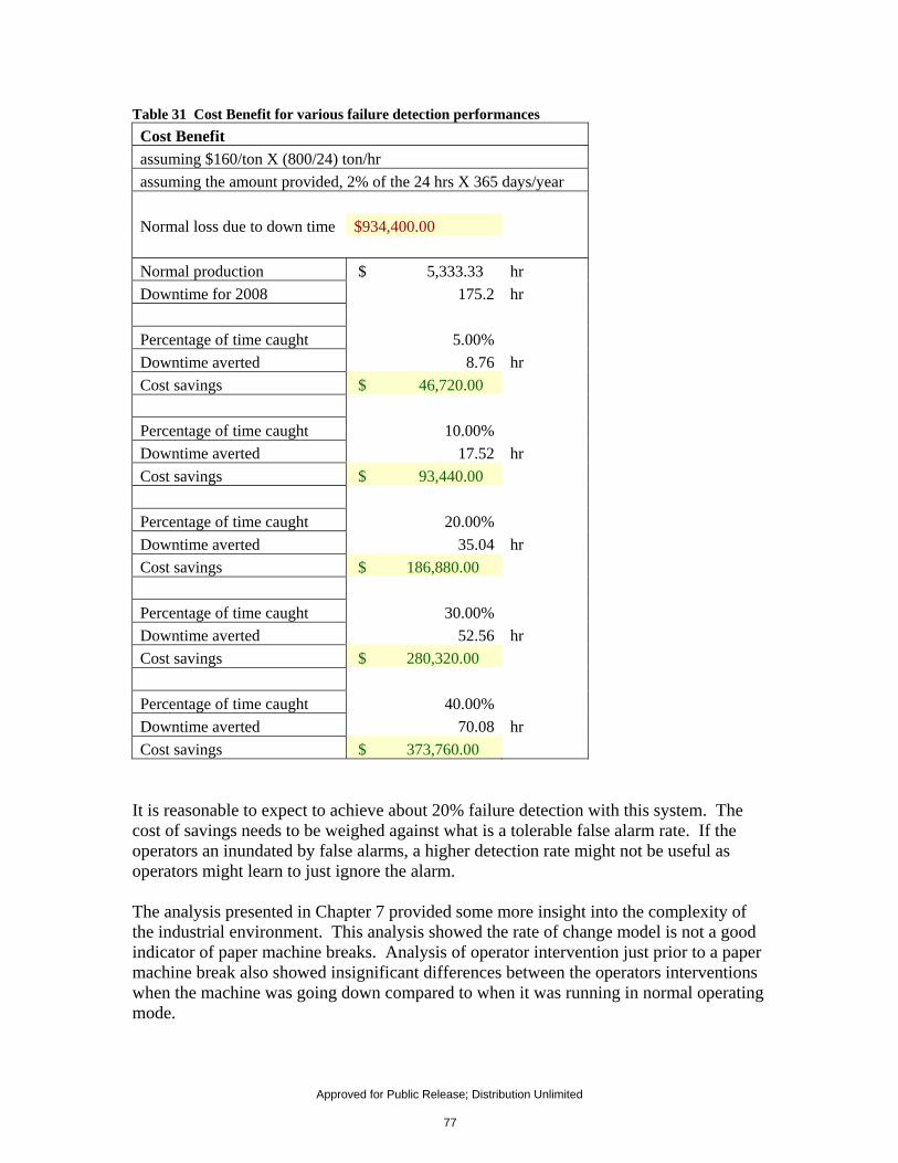
Table 31 Cost Benefit for various failure detection performances Cost Benefit assuming $160/ton X (800/24) ton/hr assuming the amount provided, 2% of the 24 hrs X 365 days/year Normal loss due to down time $934,400.00 Normal production $ 5,333.33 hr Downtime for 2008 175.2 hr Percentage of time caught 5.00% Downtime averted 8.76 hr Cost savings $ 46,720.00 Percentage of time caught 10.00% Downtime averted 17.52 hr Cost savings $ 93,440.00 Percentage of time caught 20.00% Downtime averted 35.04 hr Cost savings $ 186,880.00 Percentage of time caught 30.00% Downtime averted 52.56 hr Cost savings $ 280,320.00 Percentage of time caught 40.00% Downtime averted 70.08 hr Cost savings $ 373,760.00

It is reasonable to expect to achieve about 20% failure detection with this system. The cost of savings needs to be weighed against what is a tolerable false alarm rate. If the operators an inundated by false alarms, a higher detection rate might not be useful as operators might learn to just ignore the alarm. The analysis presented in Chapter 7 provided some more insight into the complexity of the industrial environment. This analysis showed the rate of change model is not a good indicator of paper machine breaks. Analysis of operator intervention just prior to a paper machine break also showed insignificant differences between the operators interventions when the machine was going down compared to when it was running in normal operating mode.


The models and tools explored in this research could be implemented successfully in an industrial environment to serve as a much needed virtual advisor to the operators. Such a system could not only advise the operators of the various actions to be taken to keep the process running in a stable fashion, they could also minimize the probability of paper machine downtimes. It could help mill engineers indentify sources of variability in the process and allow them to improve the overall process runnability.

8.2 Future Direction

8.2.1 Basic Research The future direction of this research effort is to apply the tools and methods investigated within this research to the military domain. Some basic research which warrants further investigation is described below. The QT-KMeans models varied the size of the sphere which characterized the clusters. Another method for adjusting the clusters is through changing the shape of the clusters. This can be accomplished with such tools such as self organizing feature maps. Also, the threshold values on the QT-Models were adjusted manually. An algorithm which could optimize competing objective functions could allow the operator to enter a sensitivity value and the thresholds adjustments could be automatic. Another area of future work is in model fusion. Model fusion would involve extracting the information from multiple predictive models and using this information to formulate a better prediction. Unrelated to software tools, general maintenance issues should be addressed. Some sensors may need to be upgraded, equipment may need to be calibrated, and tighter control may be needed to reduce process variability. Another area for potential process improvement would be tighter quality control of the raw material coming in to the system.

8.2.2 Applied Research An additional application of the methods and techniques presented in this research is in space situational awareness. The Space Surveillance Network currently detects, tracks, and catalogs approximately 22,000 objects. It is estimated that the addition of new sensing capabilities from SST, Space Fence, and SBSS may increase detected objects by an order of magnitude. It is impossible for analysts to manually process data on all new objects. New techniques are required to sort through the growing volumes of data to identify possible objects of interest from hundreds of thousands of detections and judiciously designate these objects for further SSN sensor tasking and assessment. Automated algorithms are needed to help


find the "needles in the haystack" to reduce time analysts spend doing tedious tasks and enable them to focus their attention to the most important tasks. The methods developed in this research were applied to an industrial data set which took vast amounts of multiple sensor inputs laden with data discrepancies and uncertainty. There was also a time dependency in the data that needed to be considered. This real-world data set shared many similarities to sensor inputs in the space based domain. The novel research in the methods investigated is in further developing a pattern matching technique called the Quality Threshold Model (QTM) and applying it to challenges in the space domain. The model is an event prediction tool that provides adjustable thresholds for various anomalies. It is based on a layered learning approach that 1) uses data mining methods to sort through vast amounts of data, 2) pre-filter and preprocessing to help identify key features which characterize the objects of interest and analyze the quality and temporal aspects of the data, and 3) apply pattern matching and semi-supervised learning tools to assist the end user in space object discrimination so that they may better identifying anomalies of interest.


9 BACK MATTER

9.1 Appendix A - Java-ML Method For Accessing Centroids // ----< average >---------------------------------------------------- // /** * Creates an instance that contains the average values for the attributes. * Had to write this because the "average" method in the java-ml library did * mid range and not arithmetic mean. * * @param data * data set to calculate average attribute values for * @return Instance representing the average attribute values */ public static Instance average(Dataset data) { if (data.size() < 1) { throw new IllegalArgumentException( "Dataset has to have at least one Instance in it."); } // end if int instCnt = data.size(); Instance avg = new DenseInstance(data.get(0).noAttributes()); int attribCnt = avg.noAttributes(); int t = 1; for (int i = 0; i < instCnt; i++) { Instance inst = data.get(i); double oneOverT = 1.0 / t; double tMinus1OverT = ((double)t - 1) / t; for (int j = 0; j < attribCnt; j++) { double val = inst.get(j); avg.put(j, (tMinus1OverT * avg.get(j)) + (oneOverT * val)); } // end for t++; } // end for return avg; } // end average // ----< standardDeviation >------------------------------------------ // /** * Actually "bias connected sample standard deviation". */ public static Instance standardDeviation(Dataset data, Instance avg) { Instance sum = new DenseInstance(new double[avg.noAttributes()]); for (Instance i : data) { Instance diff = i.minus(avg); sum = sum.add(diff.multiply(diff)); } sum = sum.divide(data.size()-1); return sum.sqrt(); } // end standardDeviation


Excerpt from MyKMeans.java, the modification to the KMeans.java file in the Java-ML library. /** * This method only calculates the clusters of a data set, it doesn't have * the overhead of putting all the data into cluster datasets. * * @param data */ public void clusterOnly(Dataset data) { if (data.size() == 0) throw new RuntimeException("The dataset should not be empty"); if (numberOfClusters == 0) throw new RuntimeException("There should be at least one cluster"); // Place K points into the space represented by the objects that are // being clustered. These points represent the initial group of // centroids. // DatasetTools. Instance min = DatasetTools.minAttributes(data); Instance max = DatasetTools.maxAttributes(data); this.centroids = new Instance[numberOfClusters]; int instanceLength = data.instance(0).noAttributes(); for (int j = 0; j < numberOfClusters; j++) { double[] randomInstance = new double[instanceLength]; for (int i = 0; i < instanceLength; i++) { double dist = Math.abs(max.value(i) - min.value(i)); randomInstance[i] = (float) (min.value(i) + rg.nextDouble() * dist); } // end for this.centroids[j] = new DenseInstance(randomInstance); } // end for int iterationCount = 0; boolean centroidsChanged = true; boolean randomCentroids = true; while (randomCentroids || (iterationCount < this.numberOfIterations && centroidsChanged)) { // System.out.println("Performing iteration: " + iterationCount); iterationCount++; // Assign each object to the group that has the closest centroid. int[] assignment = new int[data.size()]; for (int i = 0; i < data.size(); i++) { int tmpCluster = 0; // double minDistance = dm.measure(centroids[0], data.instance(i)); double minDistance = dm.measure(data.instance(i), centroids[0]); for (int j = 1; j < centroids.length; j++) { // double dist = dm.measure(centroids[j], data.instance(i)); double dist = dm.measure(data.instance(i), centroids[j]); if (dm.compare(dist, minDistance)) { minDistance = dist; tmpCluster = j; } // end if } // end for assignment[i] = tmpCluster; } // end for // When all objects have been assigned, recalculate the positions of // the K centroids and start over. // The new position of the centroid is the weighted center of the


// current cluster. double[][] sumPosition = new double[this.numberOfClusters][instanceLength]; int[] countPosition = new int[this.numberOfClusters]; for (int i = 0; i < data.size(); i++) { Instance in = data.instance(i); for (int j = 0; j < instanceLength; j++) { sumPosition[assignment[i]][j] += in.value(j); } // end for countPosition[assignment[i]]++; } // end for centroidsChanged = false; randomCentroids = false; for (int i = 0; i < this.numberOfClusters; i++) { if (countPosition[i] > 0) { double[] tmp = new double[instanceLength]; for (int j = 0; j < instanceLength; j++) { tmp[j] = (float) sumPosition[i][j] / countPosition[i]; } // end for Instance newCentroid = new DenseInstance(tmp); if (dm.measure(newCentroid, centroids[i]) > 0.0001) { centroidsChanged = true; centroids[i] = newCentroid; } // end if } else { double[] randomInstance = new double[instanceLength]; for (int j = 0; j < instanceLength; j++) { double dist = Math.abs(max.value(j) - min.value(j)); randomInstance[j] = (float) (min.value(j) + rg.nextDouble() * dist); } // end for randomCentroids = true; this.centroids[i] = new DenseInstance(randomInstance); } // end if } // end for } // end while } // end clusterOnly /** */ public Dataset[] cluster(Dataset data) { // do the clustering work clusterOnly(data); Dataset[] output = new Dataset[centroids.length]; for (int i = 0; i < centroids.length; i++) { output[i] = new DefaultDataset(); } // end for for (int i = 0; i < data.size(); i++) { int tmpCluster = 0; // double minDistance = dm.measure(centroids[0], data.instance(i)); double minDistance = dm.measure(data.instance(i), centroids[0]); for (int j = 0; j < centroids.length; j++) { // double dist = dm.measure(centroids[j], data.instance(i)); double dist = dm.measure(data.instance(i), centroids[j]); if (dm.compare(dist, minDistance)) { minDistance = dist; tmpCluster = j; } // end if } // end for


output[tmpCluster].add(data.instance(i)); } // end for return output; } // end cluster


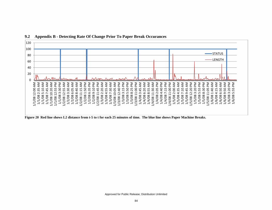
9.2 Appendix B - Detecting Rate Of Change Prior To Paper Break Occurances

Figure 20 Red line shows L2 distance from t-5 to t for each 25 minutes of time. The blue line shows Paper Machine Breaks.

0

20

40

60

80

100

120

1/1/08

12:00

AM

1/1/08

2:35 AM

1/1/08

5:10 AM

1/1/08

7:45 AM

1/1/08

10:20

AM

1/1/08

12:55

PM

1/1/08

3:30 PM

1/2/08

12:55

AM

1/2/08

3:30 AM

1/2/08

6:05 AM

1/2/08

8:40 AM

1/2/08

11:15

AM

1/2/08

1:50 PM

1/2/08

6:35 PM

1/2/08

9:10 PM

1/2/08

11:45

PM

1/3/08

2:20 AM

1/3/08

4:55 AM

1/3/08

7:30 AM

1/3/08

10:05

AM

1/3/08

12:40

PM

1/3/08

3:15 PM

1/3/08

5:50 PM

1/3/08

8:25 PM

1/3/08

11:00

PM

1/4/08

3:45 AM

1/4/08

6:20 AM

1/4/08

8:55 AM

1/4/08

11:30

AM

1/4/08

2:05 PM

1/4/08

4:40 PM

1/4/08

7:15 PM

1/4/08

11:00

PM

1/5/08

2:00 AM

1/5/08

4:35 AM

1/5/08

7:10 AM

1/5/08

9:45 AM

1/5/08

12:20

PM

1/5/08

3:20 PM

1/5/08

5:55 PM

1/5/08

8:30 PM

1/5/08

11:05

PM

1/6/08

1:40 AM

1/6/08

4:15 AM

1/6/08

6:50 AM

1/6/08

9:50 AM

1/6/08

3:20 PM

1/6/08

5:55 PM

STATUS

LENGTH


Figure 21 Red line shows L2 distance from t-5 to t for each 25 minutes of time. The blue line shows Paper Machine Breaks.

0

20

40

60

80

100

1201/27

/08 11

:10 AM

1/27

/08 1:50

PM

1/27

/08 5:40

PM

1/27

/08 8:20

PM

1/27

/08 11

:00 PM

1/28

/08 1:40

AM

1/28

/08 4:20

AM

1/28

/08 7:00

AM

1/28

/08 9:40

AM

1/28

/08 12

:20 PM

1/28

/08 3:00

PM

1/28

/08 7:35

PM

1/28

/08 10

:15 PM

1/29

/08 12

:55 AM

1/29

/08 8:05

AM

1/29

/08 10

:45 AM

1/29

/08 1:25

PM

1/29

/08 4:05

PM

1/29

/08 6:45

PM

1/29

/08 9:25

PM

1/30

/08 12

:05 AM

1/31

/08 2:15

PM

1/31

/08 4:55

PM

1/31

/08 9:55

PM

2/1/08

12:35

AM

2/1/08

3:15 AM

2/1/08

5:55 AM

2/1/08

8:35 AM

2/1/08

11:15

AM

2/1/08

4:30 PM

2/1/08

8:30 PM

2/1/08

11:10

PM

2/2/08

1:50 AM

2/2/08

4:30 AM

2/2/08

7:10 AM

2/2/08

9:50 AM

2/2/08

12:30

PM

2/2/08

3:10 PM

2/2/08

5:50 PM

2/2/08

8:30 PM

2/3/08

1:30 AM

2/3/08

6:15 AM

2/3/08

12:10

PM

2/3/08

4:35 PM

2/3/08

7:15 PM

2/3/08

9:55 PM

2/4/08

12:35

AM

STATUS

LENGTH


9.3 List of Acronyms PI System Plant Information System ML Machine Learning ANN Artificial Neural Network KNN K-Nearest Neighbor PM Paper Machine QT Quality Threshold GUI Graphical User Interface PID Proportional, Integral, Derivative P&ID Plant and Instrumentation Diagram


10 BIBLIOGRAPHY 1. Kappen, J. Modelling and Simulation in the Paper Industry. s.l. : COST Aciton E36, 2006. 2. Chiang, L., Russell, E., and Braatz, R. Fault Detection and Diagnosis in Industrial Systems. Great Britain : Springer-Verlag London Limited, 2001. 3. Basir, O.A., Shen, H.C. Modeling and fusing uncertain multisensory data. J. Robot Syst. 1996, Vol. 13, 2, pp. 95-109. 4. Hatzipantellis, E., Murray, A., Penman, J. Comparing Hidden Markov Models with artificial neural networks for condistion monitoring applications. Proc. Artificial Neural Networks. June 1995, pp. 369-374. 5. Iserman, R. Process fault detection based on modeling and estimation methods. Automatica. 1984, Vol. 20 , 4, pp. 397-404. 6. Wei, W. Time Series Analysis Univariant and Multivariant Methods. Redwood City, CA : Addison-Wesley, 1990. 7. Basseville, M., Nikiforov, V. Detection of Abrupt Changes, Theory and Application. Englewood Cliffs : Prentice-Hall, 1993. 8. Kim, B., and May, G.S. Real-time diagnosis of semiconductor manufacturing equipment using a hybrid neural network expert system. IEEE Trans. Com., Packag., Manufact. technol. conference. Jan. 1997, pp. 39-47. 9. Baker, M., himmel, C., and May, G. Time series modeling of reactive ion etching using neural networks. IEEE Trans. Semiconduct. Manufacturing. Feb. 1995, Vol. 8, pp. 62-71. 10. Weigend, A., Gershenfeld,N. Time Series Prediction: Forcasting the Future and Understanding the Past. Reading, MA : Addison-Wesley, 1994. 11. Scott, G. Knowledge-based artificial neural networks for process modeling and control. s.l. : The University of Wisconsin, 1993. 12. Hill, T. and Lewicki, P. Statistics Methods and Applications. Tulsa, OK : StatSoft Inc., 2007. 13. OSIsoft - The PI System: Empowering business in real-time. [Online] OSIsoft. http://www.osisoft.com/Default.aspx. 14. Grades of Pulp and Paper. [Online] PaperOnWeb. [Cited: ] http://www.paperonweb.com/grade.htm. 15. Grades of Pulp and Paper. PaperOnWeb. [Online] [Cited: November 27, 2007.] http://www.paperonweb.com/grade.htm. 16. Hagedorn, A., Orccotoma, J., Schueler P., Snow, B., and Jarvinen, J. Optimizing Machine Efficiency Through Fibre Quality Management. Conference Proceedings, Papermaker's Conference. 2006. 17. Set, R. Fibre Quality Factors in Pulps I: The Importance of Fibre Length and Strength. Paprican. March 1990. 18. Smook, G.A. Handbook for pulp and paper technologist. Vancouver : Angus Wilde Publications, 1992. 19. How is Paper Recycled. [Online] [Cited: October 14, 2009.] http://www.tappi.org/paperu/all_about_paper/earth_answers/EarthAnswers_Recycle.pdf. 20. Thorpe, B.A. Paper Machine Operations (The Pulp and Paper Manufacture Series, Vol 7). Atlanta : Tappi, 1997.


http://www.osisoft.com/Default.aspx

http://www.paperonweb.com/grade.htm

http://www.paperonweb.com/grade.htm

http://www.tappi.org/paperu/all_about_paper/earth_answers/EarthAnswers_Recycle.pdf

21. Perkins, J. Brown Stock Washing. [book auth.] T., and Malcolm, E. Grace. Pulp and Paper Manufacture: Alkaline Pulping. Atlanta : TAPPI, 1996, Vol. 5, pp. 279-317. 22. Mittal, A. A study of dissolved solids buildup with effluent recycle in a paperboard mill. Syracuse : Dissertation SUNY ESF, 2004. 23. Browning, B.L. The Nature of Paper. [book auth.] J.P. Casey. Pulp and Paper: Chemistry and Chemical Technology. New York : John Wiley & Sons, 1981. 24. Cutshall, K. Cross Directional Control. [book auth.] B.A. Thorp. [ed.] M. J. Kocurek. Pulp and Paper Manufacture: Volume 7: Paper Machine Operations. Atlanta : Tappi, 1991, 7. 25. Thake, A.J., Forbes, J.F. McLellan, P.J. Design of filter-based controllers for cross-directional contol of paper machines. Proceedings of the American Control Conference. June 1997, Vol. 3, pp. 1488-1493. 26. Wang, X.G., Dumont, G.A., Davies, M.S. Modeling and identifications of basis weight variations in paper machines. IEEE Transactions on Control Systems Technology. 1993, Vol. 1, 4, pp. 230-237. 27. Zhu, Yucai. Multivariable System Identification for Process Control. s.l. : Elsevier Science Ltd., 2001. 28. Hughes, T. Measurement and Control Basics. s.l. : ISA, 2006. 29. Perlmutter, D. Introduction to Chemical Process Control. New York : John Wiley & Sons, Inc., 1965. 30. Smith, C. and Corripi, A. Principles and Practice of Automatic Process Control. New York : John Wiley & Sons, 1985. 31. Zhang, Z., Jia, L., Chai, Y. Research on Elementary Principals of Complex System Control. Proceedings from the IEEE 3rd International Conference on Innovative Computing Information. 2008. 32. Heylighen, F. Evolutionary transitions: how do levels of complexity emerge? Complexity. 2000, Vol. 6, 1, pp. 53-57. 33. Wang, C., Wang, F., He, J. Some key issues in studying complex systems. Control Theory and Applications. 22, August 2005, Vol. 4, pp. 604-608. 34. Katz, M. H. Multivariable Analysis: A primer for readers of medical research. Ann Intern Med. 2003, Vols. 138: 644-50. 35. Anderson, T. An Introduction to Multivariate Statistical Analysis. Hoboken, New Jersey : John Wiley & Sons, Inc., 2003. 36. Weber, W., DiGiano, F. Process Dynamics in Environmental Systems. New York, NY : John Wiley & Sons, Inc., 1996. 37. Marlin, T. Process Control: Designing Processes and Control Systems for Dynamic Performance. New York, New York : McGraw-Hill, 2000. 38. Russell, S., Norvig, P. Artificial Intelligence: A Modern Approach. Upper Saddle River : Prentice Hall, Inc, 1995. 39. Woodward, J. Computable and incomputable functions and search algorithms. Intelligent Computing and Intelligent Systems. November 2009, Vol. 1, pp. 871-875. 40. Wolpert, D.H. The lack of a priori distictions between learning algorithms. Neural Computation. 1996, Vol. 8, 7, pp. 1341-1390. 41. Zhu, H. No free lunch for cross validation. Neural Computation. Vol. 8, 7, pp. 1421-1426.


42. Mehrotra, K. Mohan, C., Ranka, S. Elements of Artificial Neural Networks. Cambridge : The MIT Press, 2000. 43. Baum, E. and Wilczek, F. Supervised learning of probability distributions by neural networks. Neural Information Processing Systems. 1988, pp. 52-61. 44. Documentation- Neural Network Toolbox. Mathworks. [Online] [Cited: January 13, 2010.] http://www.mathworks.com/access/helpdesk/help/toolbox/nnet/neuron_2.html#33674. 45. Sharkely, A. Combining Artificial Neural Nets. London : Springer, 1999. 46. Barlow, H.B. Unsupervised Learning. Neural Computation. 1989, Vol. 1, 3, pp. 295-311. 47. Barlow, H. Possible principles underlying the transformations of sensory messages. [book auth.] W. Rosenblith. Sensory Communication. Cambridge, MA : MIT Press, 1961. 48. Lei, X. Data Mining, unsupervised learning and Bayesian ying-yang theory. International Joint Conference on Neural Networks. July 1999, Vol. 4, pp. 2520-2525. 49. Fayyad, U. Advances in Knowledge Discovery and Data Mining. s.l. : AAAI/MIT Press, 1996. 50. Brachman, R., Khabaz, T., Kloesgen, W., Piatetsky, S., and Simoudis, E. Industrial Applications of Data Mining and Knowledge Discovery. Communications of ACM. 1996, Vol. 39, 11. 51. Luo, Q. Advancing Knowledge Discovery and Data Mining. IEEE Workshop on Knowledge Discovery and Data Mining. 2008. 52. Li, Z., Yuan, J., Yang, H. Khang, K. K-mean Algorithm with a Distance Based on Characteristics of Differences. 4th International Conference on Wireless Communications, Networking and Mobile Computing. Oct 2008, pp. 1-4. 53. Myatt, G. Making Sense of Data: A Practical Guide to Exploratory Data Analysis and Data Mining. s.l. : John Wiley & Sons, Inc., 2007. 54. Lin, N., Chang, C., Chueh, H., Chen, H., Hao, W. A deflected grid-based algorithm for clustering analysis. WSEAS Transactions on Computers. 2008, Vol. 7, 4, pp. 125-132. 55. Lipkovich, I. and Smith E. Model Based Cluster and Outlier Analysis. [Online] 2003. [Cited: Feb 2, 2010.] http://www.web-e.stat.vt.edu/dept/web-e/smith/ModelBasedCluster.pdf. 56. Han, J. and Kamber, M. Data Mining: Concepts and Techniques. San Diego : Academic Press, 2001. 57. MacQueen, J. Some methods for classification and analysis of multivariate observations. Proc. 5th Berkeley Symp. Mat. Statist, Prob. 1967, Vol. 1, pp. 281-297. 58. Duda, R., Hart, P., Stork, D. Pattern Classification. New York : John Wiley & Sons, Inc., 2001. 59. Pang-Ning, T, Steinbach, M., and Kumar, V. Introduction to Data Mining . s.l. : Addison-Wesley, 2005. 60. Yu, J., Amores, J., Sebe, N., Radeva, P. and Tian, Q. Distance Learning for Similarity Estimation. IEEE Transactions of Pattern Analysis and Machine Intelligence. March 2008, Vol. 30, 3, pp. 451-462. 61. Domeniconi, C., Peng, J. Gunopulos, D. Locally Adaptive Metric Nearest Neighbor Classification. IEEE Trans. Pattern Analysis and Machine Intelligence. Sept. 2002, Vol. 24, 9, pp. 1281-1285.


http://www.mathworks.com/access/helpdesk/help/toolbox/nnet/neuron_2.html#33674

http://www.web-e.stat.vt.edu/dept/web-e/smith/ModelBasedCluster.pdf



62. Xing, E., Ng, A., Jordan, M., and Russell, S. Distance Metric Learning, with Application to Clustering with Side-Information. Proc. Neural Information Processing Systems. 2003, pp. 505-512. 63. MacQueen, J. Cluster analysis. widipedia. [Online] http://en.wikipedia.org/wiki/Cluster_analysis#cite_note-0. 64. Exploring Expression Data: Identification and Analysis of Coexpressed Genes. Heyer, L., et al. 1999, Genome Research, Vol. 9, pp. 1106-1115. 65. Zadeh, L. "Fuzzy Sets". Information and Control. 1965, Vol. 8, pp. 338-353. As sited by Martin. 66. Data Mining Technology applications in the Pulp and Paper Industry. Mustonen, M. 2005. Papermakers Conference. 67. Lennoz, B. Rutherford, P., Montague, A., Haughnin, C. Case study investigating the application of neural networks for process modelling and condition monitoring. Computers & Chemical Engineering. 1998, Vol. 22, pp. 1573-1579. 68. Belarbi, K., Bettou, K., Mezaache, A.,. Fuzzy neural networks for estimation and fuzzy contoller design: simulation for a pulp batch digester. Journal of Process Control. 2000, Vol. 10, pp. 35-41. 69. Alexandridis, A., Sarimveis, H., Bafas, G., Restsina, T. A neural network approach for modelling and control of continuous digesters. TAPPI Fall Technical Conference. 2002. 70. Dung, P., Phuong, L. ANN-Contol System DC Motor. IEEE Transacations. pp. 82-90. 71. El-Sharkawi, M., Weerasooriya, S. Identification and control of a dc motor using back-propagation neural networks. IEEE Transactions on energy conversion. 1991, Vol. 6, pp. 663-669. 72. Kotaru, R. Rubai, A. Online Identification and control of a dc motor using learning adaptation of neural networks. IEEE Transactions on industry applications. June 2000, Vol. 36, pp. 935-942. 73. Liu, Z., Zhuang, X., Wang, S. Speed Control of a DC Motor using BP Neural Networks. IEEE Transactions. pp. 832-835. 74. Cajueiro, D, Hemerly, E. Direct Adaptive Control using Feedforward Neural Networks. Revista Control and Automation. December 2003, Vol. 14, pp. 348-358. 75. Franklin, J.A. Three applications of artificial neural networks for control. IEEE International Conference on Neural Networks. 1993, Vol. 2, pp. 737-742. 76. Curty da Motta Lima, O., Curvelo Pereira, Nehemias , andDeganutti, F. Study of the multicylinder dyring section of the Klabin-PR MP7 papermachine. TAPPI Journal. December 2005, Vol. 4, 12. 77. Huang, B. and Mujumdar, A. Drying Technology. 1993, Vol. 11, 3, p. 525. As cited by Lima et al.. 78. Retsina, T., Rutherford, S., Panagiotis, P. Neural Network Model-Based Paper Machine Marginal Cost Curves. TAPPI Engineering, Pulping & Environmental Conference Proceesings. 2005. 79. Rubini, B., Yamamoto, C. Development of predictive oxygen delignification models using kinetic expressions and neural netowrks. TAPPI Journal. May 2006, Vol. 5, 4, pp. 3-6.


http://en.wikipedia.org/wiki/Cluster_analysis#cite_note-0

80. Kooi, S. and Khorasani, K. Control of the woodchip refiner using neural networks. TAPPI Journal. June 1992, Vol. 75, 6, pp. 157-162. 81. Vaughan, J., Gottlieb, P., Lee, S., and Beilstein, J. Development of a Neural Network Soft Sensor for Chlorine Dioxide Brightness Control. Conference Proceedings on Process Corntrol. 1999. 82. Miyanishi, T. and Shimada, H. Neural Networks in Web Break Diagnosis of a Newsprint Paper Machine. 1997 Papermakers Conference Proceedings. 83. Smity, G., Wrobel, C., and Stengel, D. Modeling trs and so2 emissions from a kraft recovery boiler using artificial neural networks. TAPPI Journal. November 2000, Vol. 83, 11, pp. 1-11. 84. Baines, G., Hayes, R., Stabell, J. Predicting boiler emissions with neural networks. TAPPI Journal. May 1997, Vol. 80, 5, pp. 58-61. 85. m-Track - Monitoring time-varying relations in approximately categorized knowledge. Martin, T., Shen, Yun. 2009. IEEE Symposium on Computational Intelligence for Security and Defense Applications. pp. 1-8. 86. Attack your paper making issues with CAT (cluster analysis tool). Cason, J. s.l. : Papermakers Conference, 2006. 87. Sutanto. E., Warwick, K. Multivariable cluster analysis for high speed industrial machinery. IEEE Proceedings- Science, Measurement, and Technology. September 1995, Vol. 142, 5, pp. 417-423. 88. Skormin, V., Popyack, L., Gorodetski, V., Araiza, M., Michel, J. Applications of Cluster Analysis in Diagnostics Related Problems. 89. Bown, M. and Harris, C. Neurofuzzy Adaptive Modelling and Control. 1994. 90. Lehmann, E.L. and D'Abrera, H. Nonparametrics: Statistical Methods Based on Ranks, rev. ed. Englewood Cliffs : Prentice-Hall, 1998. 91. NeurOn-Line Studio User's Guide. s.l. : Gensym Corporation, 2007. 92. Fault Detection Using the K-Nearest Neighbor Rule for Semiconductor Manufacturing Processes. Peter, Q., Wang, J. 4, November 2007, IEEE Transactions on Semiconductor Manufacturing, Vol. 20. 93. Abeel, T. http://java-ml.sourceforge.net/. Java-ML Library. [Online] 94. Abel, T., Van de Peer, Y., Saeys, Y. Java-ML: A Machine Learning Library. Journal of Machine Learning Research. 2009, Vol. 10, pp. 931-934. 95. Determination of Number of Clusters in K-Means Clustering and Application in Color Image Segmentation. Ray, S., and Turi, R. Calcutta, India : s.n., 1999, Proceedings of the Fourth International Conference on Advances in Pattern Recognition and Digital Techniques, pp. 137-143. 96. Prediction of Moving Objects' K-Nearest Neighbor Based on Fuzzy-Rough Sets Theory. Haikou : s.n., 2007, Fuzzy Systems and Knowledge Discovery, 2007. FSKD 2007. Fourth International Conference on , Vol. 1. 97. Smyth, P. Hidden Markov Models and Neural Networks for fault detection in dynamic systems. Neural Networks for Signal Processing, III Proc. 1993 IEEE-SP Workshop. 1993, pp. 582-591. 98. Time Series Analysis Univariant and Multivariat Methods. Wei, W. W. Redwood City : Addison-Wesley, 1990. 99. Stitieler, William. Multivariate Statistics with Applicatoins in Statistical Ecology. Fairland, Maryland : International Co-operative Publishing House, 1979.


http://java-ml.sourceforge.net/

100. Rawlings, J. Tutorial overview of model predictive control. IEEE Control Systems Magazine. 2000, Vol. 20, pp. 38-52. 101. Allgower, F. Badgwell, T, Qin, S. Nonlinear predictive control and moving horizon estimation. [book auth.] P. Frank. Advances in control: highlights of ECC'99. Berlin : Springer, 1999. 102. Mayne, D., Rawlings, J., Rao, C. and Scokaert, P. Constrained model predictive control: Stability and optimality. Automatica. 2000, Vol. 36, pp. 789-814. 103. Qin, S., Badgwell, T. A survey of industrial model predictive control technology. Control Engineering Practice. July 2003, Vol. 11, 7, pp. 733-764. 104. Cohen, J., Cohen, P., West, S., Aiken, L. Applied Multiple Regression/Correlation Analysis for the Behavioral Sciences. Mahwah, New Jersey : Lawrence Erlbaum Associates, Inc., 2003. 105. Jacobs, R. Increased rates of convergence through learning rate adaptation. Neural Networks. 1988, Vol. 1, pp. 295-307. 106. Hartigan, J. Clustering Algorithms. New York : John Wiley & Sons, 1975. 107. Kaufman, L. and Rousseeuw, P. Finding Groups in Data: An Introduction to Cluster Analysis. New York : John Wiley & Sons, 1990. 108. Jain, A., Murty, M., and Flynn, J. Data clustering: A survey. ACM Comput. Surv. 1999, Vol. 31, pp. 264-323. 109. The McGraw-Hill Companies, Inc., [ed.]. McGraw-Hill Dictionary of Scientific and Technical Terms. 6.


11 PUBLICATIONS Blowers, M., “Analysis Of Machine Learning Models And Prediction Tools For Paper Machine Systems,” PhD Dissertation. SUNY College of Environmental Science and Forestry, May 2010. Blowers, M., Iribarne, J., Scott, G.,“Multi-variable analysis, correlation, and prediction,” 2009 SPIE Conference Proceedings. Blowers, M. and Sisti, A., “Evolutionary and Bio-Inspired Computation: Theory and Applications II,” Proceedings of 2008 SPIE Symposium. Oh, J., and Blowers, M., “Open Set Speaker Identification with Classifier Systems”, 2006 SPIE Defense and Security Symposium Conference Proceedings, 2006. Stipanovic, A., Blowers, M.,“Hemicellulose from Biodelignified Wood: A Feedstock for Renewable Materials and Chemicals,” American Chemical Society Symposium Series No. 921/ Feedstocks for the Future: Renewables for the Production of Chemical Materials. Chpt 16, 2005 Sabrin, H., Blowers, M., Roberts, W.J., “Target Identification Using Acoustic Signatures,” National Fire Control Symposium 2005 Conference Proceedings, 2005. Oh, J., and Blowers, M., “Text Independent Open-Set Speaker Identification for Military Missions Using Genetic Rule-Based System,” GECCO 2005 Conference Proceedings, 2005. Miller, W.J., Sezgi, A., LaRiviere, C., Blowers, M., “The TRI-Phase™ Mixer: Concept, Development, and Mill Operation,” Canadian Pulp and Paper Association Conference Papers, 1999. Miller, W.J., Blowers, M., Sezgi, A., Bardsley, D.E., “Stainless Steels for Pulp and Paper Manufacturing: Bleach Plant Section,” Publication of the Technical Association of the Pulp and Paper Industry, 1999.


DATA ANALYSIS OF COMPLEX SYSTEMS - Defense ... ANALYSIS OF COMPLEX SYSTEMS June 2011 FINAL TECHNICAL...

Documents

Transcript of DATA ANALYSIS OF COMPLEX SYSTEMS - Defense ... ANALYSIS OF COMPLEX SYSTEMS June 2011 FINAL TECHNICAL...