DARSHAN INSTITUTE OF ENGINEERING AND TECHNOLOGY Manual... · To validate Bernoulli’s Theorem as...
65
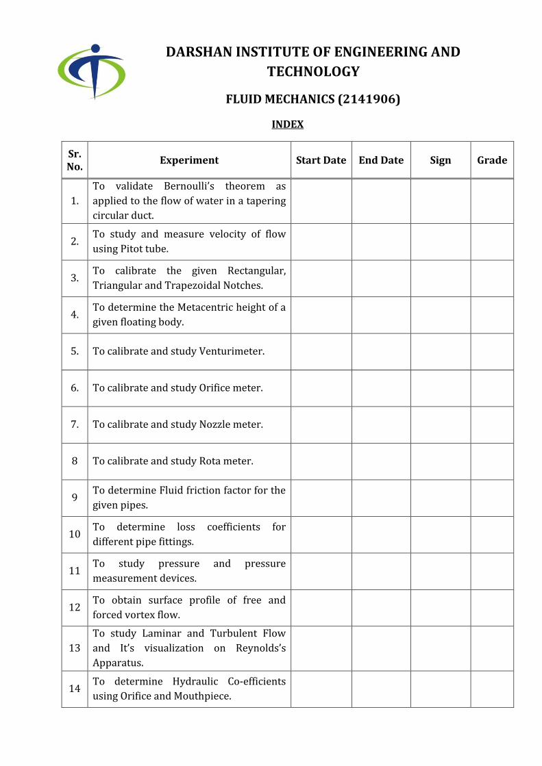
DARSHAN INSTITUTE OF ENGINEERING AND TECHNOLOGY FLUID MECHANICS (2141906) INDEX Sr. No. Experiment Start Date End Date Sign Grade 1. To validate Bernoulli’s theorem as applied to the flow of water in a tapering circular duct. 2. To study and measure velocity of flow using Pitot tube. 3. To calibrate the given Rectangular, Triangular and Trapezoidal Notches. 4. To determine the Metacentric height of a given floating body. 5. To calibrate and study Venturimeter. 6. To calibrate and study Orifice meter. 7. To calibrate and study Nozzle meter. 8 To calibrate and study Rota meter. 9 To determine Fluid friction factor for the given pipes. 10 To determine loss coefficients for different pipe fittings. 11 To study pressure and pressure measurement devices. 12 To obtain surface profile of free and forced vortex flow. 13 To study Laminar and Turbulent Flow and It’s visualization on Reynolds’s Apparatus. 14 To determine Hydraulic Co-efficients using Orifice and Mouthpiece.
Transcript of DARSHAN INSTITUTE OF ENGINEERING AND TECHNOLOGY Manual... · To validate Bernoulli’s Theorem as...
DARSHAN INSTITUTE OF ENGINEERING AND
TECHNOLOGY
FLUID MECHANICS (2141906)
INDEX
Sr. No.
Experiment Start Date End Date Sign Grade
1.
To validate Bernoulli’s theorem as
applied to the flow of water in a tapering
circular duct.
2. To study and measure velocity of flow
using Pitot tube.
3. To calibrate the given Rectangular,
Triangular and Trapezoidal Notches.
4. To determine the Metacentric height of a
given floating body.
5. To calibrate and study Venturimeter.
6. To calibrate and study Orifice meter.
7. To calibrate and study Nozzle meter.
8 To calibrate and study Rota meter.
9 To determine Fluid friction factor for the
given pipes.
10 To determine loss coefficients for
different pipe fittings.
11 To study pressure and pressure
measurement devices.
12 To obtain surface profile of free and
forced vortex flow.
13
To study Laminar and Turbulent Flow
and It’s visualization on Reynolds’s
Apparatus.
14 To determine Hydraulic Co-efficients
using Orifice and Mouthpiece.

Bernoulli’s Theorem
___________________________________________________________________________________________________
Fluid Mechanics (2141906)
Department of Mechanical Engineering
Darshan Institute of Engineering & Technology, Rajkot. 1-1
EXPERIMENT NO. 1
1.1 Objective:
To validate Bernoulli’s Theorem as applied to the flow of water in a tapering circular duct.
1.2 Introduction
Bernoulli's principle is named after the Dutch-Swiss mathematician Daniel Bernoulli who
published his principle in his book Hydrodynamica in 1738.
Bernoulli’s principle in its simplest form states that "the pressure of a fluid [liquid or gas]
decreases as the speed of the fluid increases." The principle behind Bernoulli’s theorem is
the law of conservation of energy. It states that energy can be neither created nor destroyed,
but merely changed from one form to another.
The energy, in general, may be defined as the capacity to do work. Though the energy exists
in many forms, yet the following are important from the subject point of view:
1. Potential Energy
2. Kinetic Energy and
3. Pressure Energy
1.2.1 Potential Energy of a Liquid in Motion
It is the energy possessed by a liquid particle, by virtue of its position. If a liquid particle is Z
meter above the horizontal datum (arbitrary chosen), the potential energy of liquid particle
will be gZ per kg of liquid. Potential head of the liquid, at that point, will be Z meters of the
liquid.
1.2.2 Kinetic Energy of a liquid Particle in Motion
It is the energy, possessed by a liquid particle, by virtue of its motion or velocity. If a liquid
particle is flowing with a mean velocity of V m/sec, then the kinetic energy of the particle
will be V2 2⁄ per kg of the liquid. Velocity head of the liquid, at that velocity, will be
V2 2g⁄ meter of liquid.
1.2.3 Pressure Energy of a liquid Particle in Motion
It is the energy, possessed by a liquid particle, by virtue of its existing pressure. If a liquid
particle is under a pressure of 𝑝 kg/m2, then the pressure energy of the particle will be 𝑝/𝜌
per kg of liquid, where 𝜌 is the density of the liquid. Pressure head of the liquid under that
Bernoulli’s Theorem
____________________________________________________________________________________________________
Fluid Mechanics (2141906)
Department of Mechanical Engineering
Darshan Institute of Engineering & Technology, Rajkot. 1-2
pressure will be 𝑝/𝑤 or 𝑝/𝜌𝑔 meter of the liquid. Where 𝑤 is the specific weight of the
liquid.
1.2.4 Total Energy of a liquid Particle in Motion
The total energy of a liquid particle, in motion, is the sum of its potential energy, kinetic
energy and pressure energy. Mathematically,
Total Energy, E =𝑝
𝜌𝑔+
𝑉2
2𝑔+ 𝑍, meter of liquid
1.3 Bernoulli’s Equation
It states, “For a perfect incompressible liquid, flowing in a continuous stream, the total
energy of a particle remains the same; while the particle moves from one point to another.”
This statement is based on the assumption that there are no losses due to friction in pipe.
Mathematically,
Total Energy, E =𝑝
𝜌𝑔+
𝑉2
2𝑔+ 𝑍 = Constant
1.4 Apparatus Description
The apparatus is made from transparent acrylic and has both the convergent and divergent
sections. Water is supplied from the constant head tank attached to the test section. Constant
level is maintained in the supply tank. Piezometric tubes are attached at different distance on
the test section. Water discharges to the discharge tank attached at the far end of the test
section and from there it goes to the measuring tank through valve. The entire setup is
mounted on a stand.
1.5 Experimental Procedure
1. Note down the area of cross-section of the conduit at sections where piezometers have
been fixed.
2. Open the supply valve and adjust the flow in the conduit so that the water level in the
inlet tank remains at a constant level (i.e., the flow becomes steady)
3. Measure the height of water level (above an arbitrarily selected suitable horizontal
plane) in different piezometer tubes.
4. Measure the discharge by calculating time taken for L liters flow.
5. Repeat steps (2) to (4) for other discharges.
Bernoulli’s Theorem
___________________________________________________________________________________________________
Fluid Mechanics (2141906)
Department of Mechanical Engineering
Darshan Institute of Engineering & Technology, Rajkot. 1-3
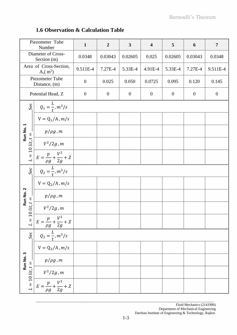
1.6 Observation & Calculation Table
Piezometer Tube
Number 1 2 3 4 5 6 7
Diameter of Cross-
Section (m) 0.0348 0.03043 0.02605 0.025 0.02605 0.03043 0.0348
Area of Cross-Section,
A,( m2) 9.511E-4 7.27E-4 5.33E-4 4.91E-4 5.33E-4 7.27E-4 9.511E-4
Piezometer Tube
Distance, (m) 0 0.025 0.050 0.0725 0.095 0.120 0.145
Potential Head, Z 0 0 0 0 0 0 0
Ru
n N
o. 1
𝐿=
10
𝑙𝑖𝑡
,𝑡=
____
____
____
Sec
𝑄1 =𝐿
𝑡, 𝑚3/𝑠
V = Q1 A⁄ , 𝑚/𝑠
𝑝 𝜌𝑔⁄ , 𝑚
𝑉2 2𝑔⁄ , 𝑚
𝐸 =𝑝
𝜌𝑔+
𝑉2
2𝑔+ 𝑍
Ru
n N
o. 2
𝐿=
10
𝑙𝑖𝑡
,𝑡=
____
____
____
Sec
𝑄2 =𝐿
𝑡, 𝑚3/𝑠
V = Q2 A⁄ , 𝑚/𝑠
𝑝 𝜌𝑔⁄ , 𝑚
𝑉2 2𝑔⁄ , 𝑚
𝐸 =𝑝
𝜌𝑔+
𝑉2
2𝑔+ 𝑍
Ru
n N
o. 3
𝐿=
10
𝑙𝑖𝑡
,𝑡=
____
____
____
Sec
𝑄3 =𝐿
𝑡, 𝑚3/𝑠
V = Q3 A⁄ , 𝑚/𝑠
𝑝 𝜌𝑔⁄ , 𝑚
𝑉2 2𝑔⁄ , 𝑚
𝐸 =𝑝
𝜌𝑔+
𝑉2
2𝑔+ 𝑍
Bernoulli’s Theorem
____________________________________________________________________________________________________
Fluid Mechanics (2141906)
Department of Mechanical Engineering
Darshan Institute of Engineering & Technology, Rajkot. 1-4
Plot the following on an ordinary graph paper for all the runs taken.
1. {(P
ρg) + z} V/s distance (x) of piezometer tubes from some reference point. Draw a
smooth curve passing through the plotted points. This is known as the Hydraulic
Gradient Line.
2. E = {(P
ρg) + z +
V2
2g} V/s distance (x) of piezometer tubes on the graph (
P
ρg) + z v/s
distance. Draw a smooth curve passing through the plotted points. This is the Total
Energy Line.
1.7 Conclusion
………………………………………………………………………………………………….
…………………………………………………………………………………………………..
………………………………………………………………………………………………….
………………………………………………………………………………………………….
…………………………………………………………………………………………………..
………………………………………………………………………………………………….
…………………………………………………………………………………………………..
Pitot Tube
____________________________________________________________________________________________________
Fluid Mechanics (2141906)
Department of Mechanical Engineering
Darshan Institute of Engineering & Technology, Rajkot.
2-1
EXPERIMENT NO. 2
2.1 Objective
To study and measure velocity of flow using Pitot tube
2.2 Introduction
A Pitot tube is a pressure measurement instrument used to measure fluid flow velocity.
The Pitot tube was invented by the French engineer Henri Pitot in the early 1700s and was
modified to its modern form in the mid 1800s by French scientist Henry Darcy. It is widely
used to determine the airspeed of an aircraft and to measure air and gas velocities in
industrial applications.
The basic Pitot tube consists of a tube pointing directly into the fluid flow. As this tube
contains fluid, a pressure can be measured; the moving fluid is brought to rest (stagnates) as
there is no outlet to allow flow to continue. This pressure is the stagnation pressure of the
fluid, also known as the total pressure or (particularly in aviation) the Pitot pressure.
The measured stagnation pressure cannot of itself be used to determine the fluid velocity
(airspeed in aviation). However, Bernoulli's equation states:
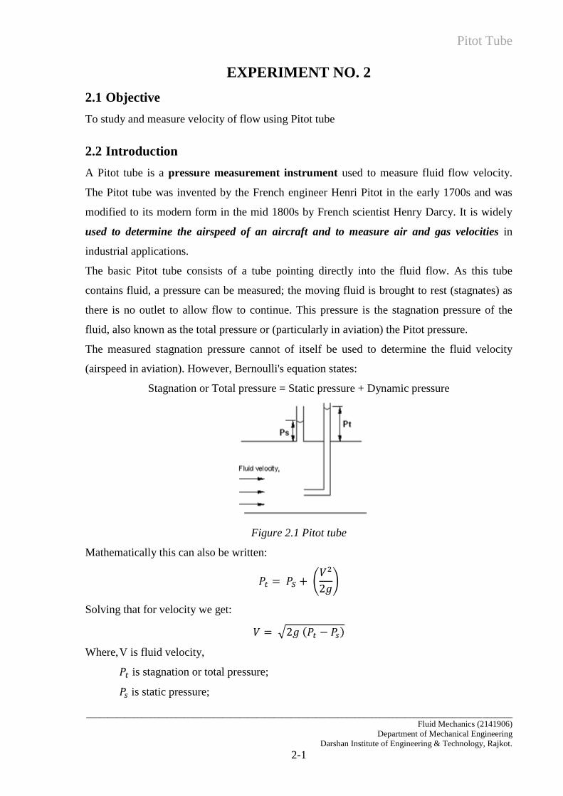
Stagnation or Total pressure = Static pressure + Dynamic pressure
Figure 2.1 Pitot tube
Mathematically this can also be written:
𝑃𝑡 = 𝑃𝑆 + (𝑉2
2𝑔)
Solving that for velocity we get:
𝑉 = √2𝑔 (𝑃𝑡 − 𝑃𝑠)
Where, V is fluid velocity,
𝑃𝑡 is stagnation or total pressure;
𝑃𝑠 is static pressure;
Pitot Tube
____________________________________________________________________________________________________
Fluid Mechanics (2141906)
Department of Mechanical Engineering
Darshan Institute of Engineering & Technology, Rajkot.
2-2
The dynamic pressure, then, is the difference between the stagnation pressure and the static
pressure.
2.3 Apparatus Description
The setup consist of simple clear Perspex channel with two tube each to measure static and
stagnation pressure of the fluid in the channel. Channel is supplied water with the help of
tank and the flow is controlled by a gate valve.
Scale is imprinted next to the tube to measure the pressure heads.
2.4 Experimental Procedure
1. Switch on the pump and feel the tank that supplies water to the Pitot apparatus.
2. Now slowly open the Pitot outlet valve so that channel is filled completely with water
3. Observe and note down the pressure heads reading in m of water
4. Calculate time for discharge for known quantity of water
5. Calculate and compare theoretical and actual velocities
2.5 Observation Table
Diameter of flow pipe, D = 0.03 m
Run No.
Total Pressure
Head
Pt, (m)
Static Pressure
Head
Ps, (m)
Dynamic Pressure
Head
(Pt − Ps), (m)
Time for L=5 lit,
t, (sec)
1
2
3
4
5
2.6 Calculations
1. Actual Discharge,
Qact = L
t=
0.005
𝑡= _________________ 𝑚3/𝑠𝑒𝑐
2. Actual Velocity,
Vact =Qact
A= _________________ 𝑚
𝑠𝑒𝑐⁄
Pitot Tube
____________________________________________________________________________________________________
Fluid Mechanics (2141906)
Department of Mechanical Engineering
Darshan Institute of Engineering & Technology, Rajkot.
2-3
3. Theoretical Velocity
Vth = √2g (Pt − Ps) = _________________ 𝑚𝑠𝑒𝑐⁄
4. Co-efficient of Pitot Tube
Cv =Vact
Vth= _________________
2.7 Result Table
Run
No.
Theoretical Velocity,
Vth, (m/sec)
Actual Discharge,
Qact, (m3/sec)
Actual Velocity,
Vact, (m/sec)
Co-efficient of
Velocity, Cv
1
2
3
4
5
2.8 Conclusion
………………………………………………………………………………………………….
…………………………………………………………………………………………………..
………………………………………………………………………………………………….
………………………………………………………………………………………………….
…………………………………………………………………………………………………..
………………………………………………………………………………………………….

Notches
____________________________________________________________________________________________________
Fluid Mechanics (2141906)
Department of Mechanical Engineering
Darshan Institute of Engineering & Technology, Rajkot.
3-1
EXPERIMENT NO. 3
3.1 Objective
To calibrate the given Rectangular, Triangular and Trapezoidal Notches
3.2 Introduction
Measurement of flow in open channel is essential for better management of supplies of water.
Notches and Weirs are used to measure the rate of flow of liquid (discharge) indirectly from
measurements of the flow depth.
Notch is a device used for measuring the rate of flow of liquid through a small channel or a
tank. It is an opening in the side of a measuring tank or reservoir extending above the free
surface. Weir is a concrete or masonry structure, placed in open channel over which the flow
occurs like a river. A notch is small in size whereas weir is a notch on a large scale.
A weir/notch is an orifice placed at the water surface so that the head on its upper edge is
zero. Hence, the upper edge can be eliminated, leaving only the lower edge named as weir
crest. A weir/notch can be of different shapes - rectangular, triangular, trapezoidal etc. A
triangular weir is particularly suited for measurement of small discharges.
Equation of discharge for notch and weir will remain same.
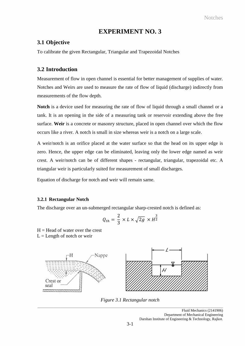
3.2.1 Rectangular Notch
The discharge over an un-submerged rectangular sharp-crested notch is defined as:
√
H = Head of water over the crest
L = Length of notch or weir
Figure 3.1 Rectangular notch
Notches
____________________________________________________________________________________________________
Fluid Mechanics (2141906)
Department of Mechanical Engineering
Darshan Institute of Engineering & Technology, Rajkot.
3-2
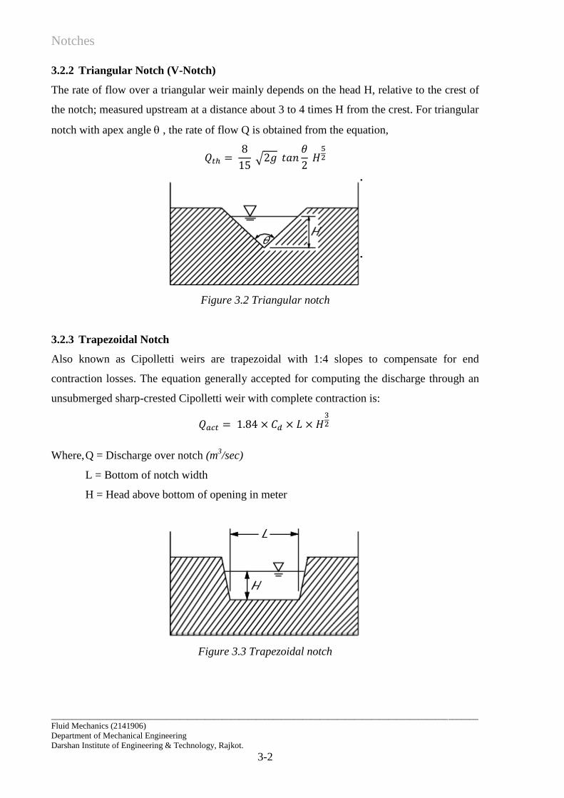
3.2.2 Triangular Notch (V-Notch)
The rate of flow over a triangular weir mainly depends on the head H, relative to the crest of
the notch; measured upstream at a distance about 3 to 4 times H from the crest. For triangular
notch with apex angle , the rate of flow Q is obtained from the equation,
√
Figure 3.2 Triangular notch
3.2.3 Trapezoidal Notch
Also known as Cipolletti weirs are trapezoidal with 1:4 slopes to compensate for end
contraction losses. The equation generally accepted for computing the discharge through an
unsubmerged sharp-crested Cipolletti weir with complete contraction is:
Where, Q = Discharge over notch (m3/sec)
L = Bottom of notch width
H = Head above bottom of opening in meter
Figure 3.3 Trapezoidal notch
Notches
____________________________________________________________________________________________________
Fluid Mechanics (2141906)
Department of Mechanical Engineering
Darshan Institute of Engineering & Technology, Rajkot.
3-3
3.3 Apparatus Description
The pump sucks the water from the sump tank, and discharges it to a small flow channel. The
notch is fitted at the end of channel. All the notches and weirs are interchangeable. The water
flowing over the notch falls in the collector. Water coming from the collector is directed to
the measuring tank for the measurement of flow.
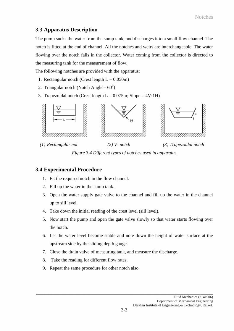
The following notches are provided with the apparatus:
1. Rectangular notch (Crest length L = 0.050m)
2. Triangular notch (Notch Angle – 600)
3. Trapezoidal notch (Crest length L = 0.075m; Slope = 4V:1H)
(1) Rectangular not (2) V- notch (3) Trapezoidal notch
Figure 3.4 Different types of notches used in apparatus
3.4 Experimental Procedure
1. Fit the required notch in the flow channel.
2. Fill up the water in the sump tank.
3. Open the water supply gate valve to the channel and fill up the water in the channel
up to sill level.
4. Take down the initial reading of the crest level (sill level).
5. Now start the pump and open the gate valve slowly so that water starts flowing over
the notch.
6. Let the water level become stable and note down the height of water surface at the
upstream side by the sliding depth gauge.
7. Close the drain valve of measuring tank, and measure the discharge.
8. Take the reading for different flow rates.
9. Repeat the same procedure for other notch also.
Notches
____________________________________________________________________________________________________
Fluid Mechanics (2141906)
Department of Mechanical Engineering
Darshan Institute of Engineering & Technology, Rajkot.
3-4
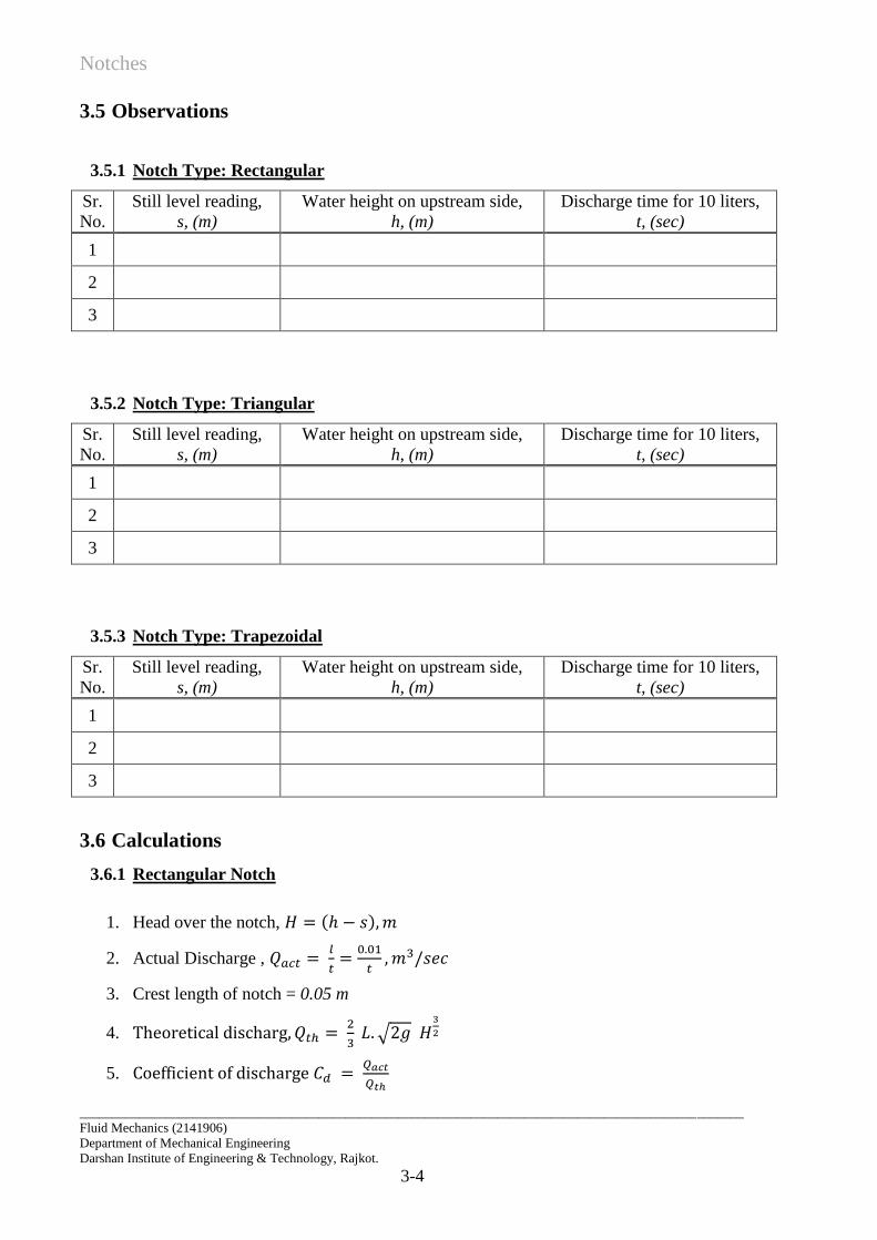
3.5 Observations
3.5.1 Notch Type: Rectangular
Sr.
No.
Still level reading,
s, (m)
Water height on upstream side,
h, (m)
Discharge time for 10 liters,
t, (sec)
1
2
3
3.5.2 Notch Type: Triangular
Sr.
No.
Still level reading,
s, (m)
Water height on upstream side,
h, (m)
Discharge time for 10 liters,
t, (sec)
1
2
3
3.5.3 Notch Type: Trapezoidal
Sr.
No.
Still level reading,
s, (m)
Water height on upstream side,
h, (m)
Discharge time for 10 liters,
t, (sec)
1
2
3
3.6 Calculations
3.6.1 Rectangular Notch
1. Head over the notch, ( )
2. Actual Discharge ,
3. Crest length of notch = 0.05 m
4.
√
5.
Notches
____________________________________________________________________________________________________
Fluid Mechanics (2141906)
Department of Mechanical Engineering
Darshan Institute of Engineering & Technology, Rajkot.
3-5
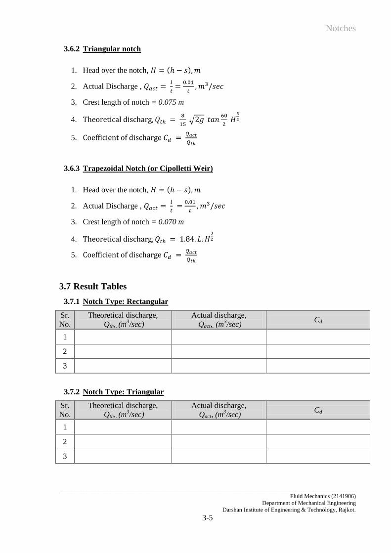
3.6.2 Triangular notch
1. Head over the notch, ( )
2. Actual Discharge ,
3. Crest length of notch = 0.075 m
4.
√
5.
3.6.3 Trapezoidal Notch (or Cipolletti Weir)
1. Head over the notch, ( )
2. Actual Discharge ,
3. Crest length of notch = 0.070 m
4.
5.
3.7 Result Tables
3.7.1 Notch Type: Rectangular
Sr.
No.
Theoretical discharge,
Qth,. (m3/sec)
Actual discharge,
Qact,. (m3/sec)
Cd
1
2
3
3.7.2 Notch Type: Triangular
Sr.
No.
Theoretical discharge,
Qth,. (m3/sec)
Actual discharge,
Qact, (m3/sec)
Cd
1
2
3
Notches
____________________________________________________________________________________________________
Fluid Mechanics (2141906)
Department of Mechanical Engineering
Darshan Institute of Engineering & Technology, Rajkot.
3-6
Notch Type: Trapezoidal
Sr.
No.
Theoretical discharge,
Qth,. (m3/sec)
Actual discharge,
Qact,. (m3/sec)
Cd
1
2
3
3.8 Conclusion
………………………………………………………………………………………………….
…………………………………………………………………………………………………..
………………………………………………………………………………………………….
………………………………………………………….……………………………………….
………………………………………………………………………………………………….
………………………………………………………………………………………………….
Metacentre
____________________________________________________________________________________________________
Fluid Mechanics (2141906)
Department of Mechanical Engineering
Darshan Institute of Engineering & Technology, Rajkot.
4-1
EXPERIMENT NO. 4
4.1 Objective
To determine the Metacentric height of a given floating body.
4.2 Buoyancy
When a body is completely submerged in a fluid, or it is floating or partially submerged, the
resultant fluid force acting on the body is called the buoyant force. It is also known as the net
upward vertical force acting on the body. A net upward vertical force results because pressure
increases with depth and the pressure forces acting from below are larger than the pressure
forces acting above.
The Center of buoyancy is the center of gravity of the displaced water. It lies at the geometric
center of volume of the displaced water.
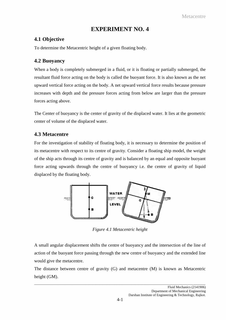
4.3 Metacentre
For the investigation of stability of floating body, it is necessary to determine the position of
its metacentre with respect to its centre of gravity. Consider a floating ship model, the weight
of the ship acts through its centre of gravity and is balanced by an equal and opposite buoyant
force acting upwards through the centre of buoyancy i.e. the centre of gravity of liquid
displaced by the floating body.
Figure 4.1 Metacentric height
A small angular displacement shifts the centre of buoyancy and the intersection of the line of
action of the buoyant force passing through the new centre of buoyancy and the extended line
would give the metacentre.
The distance between centre of gravity (G) and metacentre (M) is known as Metacentric
height (GM).
Metacentre
____________________________________________________________________________________________________
Fluid Mechanics (2141906)
Department of Mechanical Engineering
Darshan Institute of Engineering & Technology, Rajkot.
4-2
There are three conditions of equilibrium of a floating body
1. Stable Equilibrium - Metacentre lies above the centre of gravity
2. Unstable Equilibrium- Metacentre lies below the centre of gravity
3. Neutral Equilibrium - Metacentre coincides with centre of gravity
The Metacentric height (GM) is given by
𝐺𝑀 = (𝑚 𝑥 𝑋)
(𝑊 𝑥 𝑡𝑎𝑛 𝜃)
Where, W = weight of the floating body, (N)
m = movable weight, (N)
X = distance through which the movable load is shifted, (m)
= Angle of Heel
4.4 Apparatus Description
The apparatus consist of a SS tank and is provided with a drain cock. The floating body is
made from Clear Transparent Acrylic. It is provided with movable weights, protractor to
measure the angle of Heel and pointer. Weights are also provided to increase the weight of
floating body by known amount.
4.5 Experimental Procedure
1. Fill the SS tank to about 2/3 levels
2. Place the floating body in the tank.
3. Apply momentum to the floating body by moving one of the adjustable weights (m)
through a known distance.
4. Note down the angle of heel corresponding to this shifts of weight with the help of
protractor and pointer.
5. Take about 4-5 such readings by changing the position of the adjustable weight and
find out centre of gravity in each case
4.6 Observation & Result Table
Weight of the ship model = 1.5 X 9.81 = 14.715 N
Given Movable Weights = 50 gm = 0.490 N
Metacentre
____________________________________________________________________________________________________
Fluid Mechanics (2141906)
Department of Mechanical Engineering
Darshan Institute of Engineering & Technology, Rajkot.
4-3
Sr.
No.
Movable
Weight,
m, (N)
Distance of
Weight from
Center, X (m)
Angle of
Tilt, Tan
Metacentric
Height,
GM, (m)
1
2
3
4
5
4.7 Calculations
Metacentric height 𝐺𝑀 = (𝑚 𝑥 𝑋)
(𝑊 𝑥 𝑡𝑎𝑛𝜃)
Metacentric height, 𝐺𝑀 = _______________, 𝑚
4.8 Conclusion
………………………………………………………………………………………………….
…………………………………………………………………………………………………..
………………………………………………………………………………………………….
………………………………………………………………………………………………….
…………………………………………………………………………………………………..
………………………………………………………………………………………………….

Venturimeter
Fluid Mechanics (2141906)
Department of Mechanical Engineering
Darshan Institute of Engineering & Technology, Rajkot.
5-1
EXPERIMENT NO. 5
5.1 Objective
To calibrate and study Venturimeter
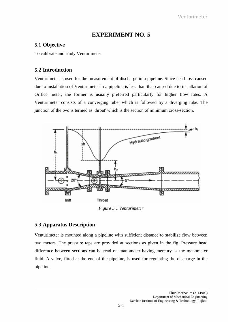
5.2 Introduction
Venturimeter is used for the measurement of discharge in a pipeline. Since head loss caused
due to installation of Venturimeter in a pipeline is less than that caused due to installation of
Orifice meter, the former is usually preferred particularly for higher flow rates. A
Venturimeter consists of a converging tube, which is followed by a diverging tube. The
junction of the two is termed as 'throat' which is the section of minimum cross-section.
Figure 5.1 Venturimeter
5.3 Apparatus Description
Venturimeter is mounted along a pipeline with sufficient distance to stabilize flow between
two meters. The pressure taps are provided at sections as given in the fig. Pressure head
difference between sections can be read on manometer having mercury as the manometer
fluid. A valve, fitted at the end of the pipeline, is used for regulating the discharge in the
pipeline.
Venturimeter
Fluid Mechanics (2141906)
Department of Mechanical Engineering
Darshan Institute of Engineering & Technology, Rajkot.
5-2
5.4 Experimental Procedure
1. Fill the storage tank/sump with the water.
2. Switch on the pump and keep the control valve fully open and close the bypass valve
to have maximum flow rate through the meter.
3. Open control valve of the Venturimeter.
4. Open the vent cocks provided at the top of the manometer to drive out the air from the
manometer limbs and close both of them as soon as water start coming out.
5. Note down the difference of level of mercury in the manometer limbs.
6. Keep the drain valve of the collection tank closed till its time to start collecting the
water.
7. Close the drain valve of the collection tank and note down the initial level of the water
in the collection tank.
8. Collect known quantity of water in the collection tank and note down the time
required for the same.
9. Change the flow rate of water through the meter with the help of control valve and
repeat the above procedure.
10. Take about 2-3 readings for different flow rates.
5.5 Observations
For Venturimeter, Diameter at inlet 𝑑1 = 26 mm; Area 𝑎1 = 5.31 x 10⁻⁴ m2
Diameter at throat 𝑑2 = 16 mm; Area 𝑎2 = 2.01 x 10⁻⁴ m2
Sr.
No
Manometric Reading Manometer Difference
(m of Hg)
𝒙 =𝒉𝟐 − 𝒉𝟏
𝟏𝟎𝟎
Time for 10 lit, t,
(sec) 𝒉𝟏 (𝒄𝒎 𝒐𝒇 𝑯𝒈) 𝒉𝟐 (𝒄𝒎 𝒐𝒇 𝑯𝒈)
1
2
3
4
5
Venturimeter
Fluid Mechanics (2141906)
Department of Mechanical Engineering
Darshan Institute of Engineering & Technology, Rajkot.
5-3
5.6 Calculations
1. Actual Discharge,
𝑄𝑎𝑐𝑡 =𝑉𝑜𝑙𝑢𝑚𝑒 𝑜𝑓 𝑊𝑎𝑡𝑒𝑟 𝑖𝑛 𝑚3
𝑇𝑖𝑚𝑒 𝑖𝑛 𝑆𝑒𝑐=
0.01
𝑡= ______________, 𝑚3 𝑠𝑒𝑐⁄
2. Difference in Pressure Head,
ℎ = 𝑥 [𝑆ℎ
𝑆𝑜− 1] = 𝑥 [
13.6
1− 1] = ______________, 𝑚 𝑜𝑓 𝑤𝑎𝑡𝑒𝑟
3. Theoretical Discharge,
𝑄𝑡ℎ =𝑎1𝑎2√2𝑔ℎ
√𝑎12 − 𝑎2
2= ______________, 𝑚3 𝑠𝑒𝑐⁄
4. Co-efficient of Discharge,
𝐶𝑑 = 𝑄𝑎𝑐𝑡
𝑄𝑡ℎ= _______________
5.7 Result Table
Sr.
No.
Theoretical Discharge,
Qth, (m3/s)
Actual Discharge,
Qact, (m3/s) Cd
1.
2.
3.
4.
5.
5.8 Conclusion
………………………………………………………………………………………………….
…………………………………………………………………………………………………..
………………………………………………………………………………………………….
………………………………………………………………………………………………….
…………………………………………………………………………………………………..

Orifice Meter
____________________________________________________________________________________________________
Fluid Mechanics (2141906)
Department of Mechanical Engineering
Darshan Institute of Engineering & Technology, Rajkot.
6-1
EXPERIMENT NO. 6
6.1 Objective
To calibrate and study Orifice meter
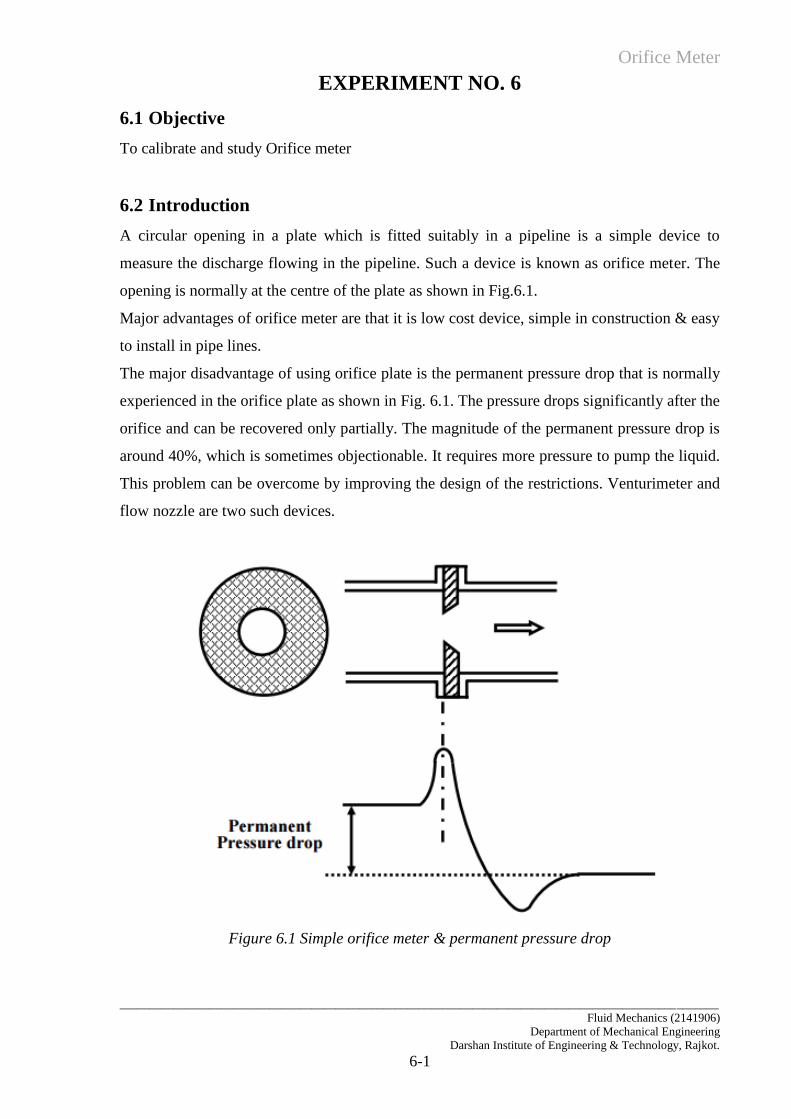
6.2 Introduction
A circular opening in a plate which is fitted suitably in a pipeline is a simple device to
measure the discharge flowing in the pipeline. Such a device is known as orifice meter. The
opening is normally at the centre of the plate as shown in Fig.6.1.
Major advantages of orifice meter are that it is low cost device, simple in construction & easy
to install in pipe lines.
The major disadvantage of using orifice plate is the permanent pressure drop that is normally
experienced in the orifice plate as shown in Fig. 6.1. The pressure drops significantly after the
orifice and can be recovered only partially. The magnitude of the permanent pressure drop is
around 40%, which is sometimes objectionable. It requires more pressure to pump the liquid.
This problem can be overcome by improving the design of the restrictions. Venturimeter and
flow nozzle are two such devices.
Figure 6.1 Simple orifice meter & permanent pressure drop
Orifice Meter
____________________________________________________________________________________________________
Fluid Mechanics (2141906)
Department of Mechanical Engineering
Darshan Institute of Engineering & Technology, Rajkot.
6-2
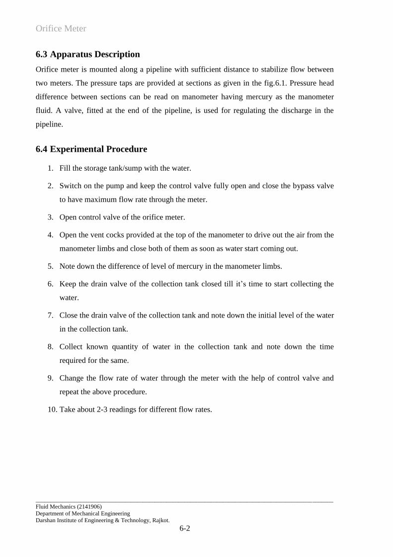
6.3 Apparatus Description
Orifice meter is mounted along a pipeline with sufficient distance to stabilize flow between
two meters. The pressure taps are provided at sections as given in the fig.6.1. Pressure head
difference between sections can be read on manometer having mercury as the manometer
fluid. A valve, fitted at the end of the pipeline, is used for regulating the discharge in the
pipeline.
6.4 Experimental Procedure
1. Fill the storage tank/sump with the water.
2. Switch on the pump and keep the control valve fully open and close the bypass valve
to have maximum flow rate through the meter.
3. Open control valve of the orifice meter.
4. Open the vent cocks provided at the top of the manometer to drive out the air from the
manometer limbs and close both of them as soon as water start coming out.
5. Note down the difference of level of mercury in the manometer limbs.
6. Keep the drain valve of the collection tank closed till it’s time to start collecting the
water.
7. Close the drain valve of the collection tank and note down the initial level of the water
in the collection tank.
8. Collect known quantity of water in the collection tank and note down the time
required for the same.
9. Change the flow rate of water through the meter with the help of control valve and
repeat the above procedure.
10. Take about 2-3 readings for different flow rates.
Orifice Meter
____________________________________________________________________________________________________
Fluid Mechanics (2141906)
Department of Mechanical Engineering
Darshan Institute of Engineering & Technology, Rajkot.
6-3
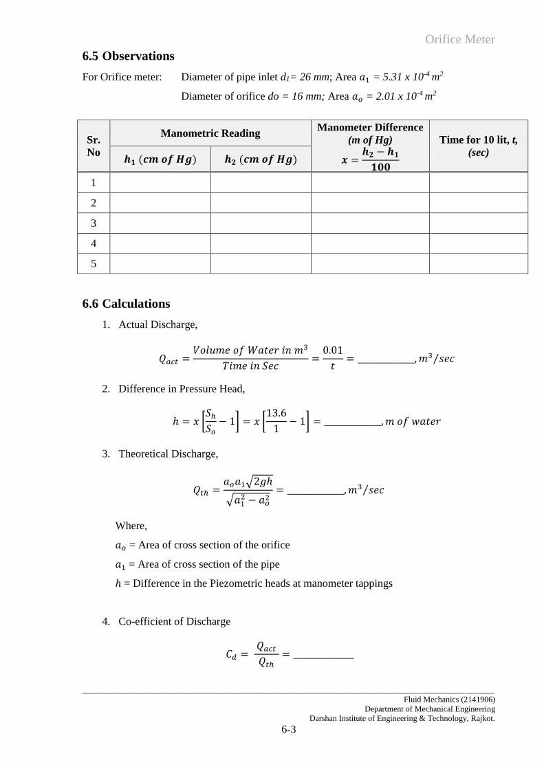
6.5 Observations
For Orifice meter: Diameter of pipe inlet d1= 26 mm; Area 𝑎1 = 5.31 x 10⁻⁴ m2
Diameter of orifice do = 16 mm; Area 𝑎𝑜 = 2.01 x 10⁻⁴ m2
Sr.
No
Manometric Reading Manometer Difference
(m of Hg)
𝒙 =𝒉𝟐 − 𝒉𝟏
𝟏𝟎𝟎
Time for 10 lit, t,
(sec) 𝒉𝟏 (𝒄𝒎 𝒐𝒇 𝑯𝒈) 𝒉𝟐 (𝒄𝒎 𝒐𝒇 𝑯𝒈)
1
2
3
4
5
6.6 Calculations
1. Actual Discharge,
𝑄𝑎𝑐𝑡 =𝑉𝑜𝑙𝑢𝑚𝑒 𝑜𝑓 𝑊𝑎𝑡𝑒𝑟 𝑖𝑛 𝑚3
𝑇𝑖𝑚𝑒 𝑖𝑛 𝑆𝑒𝑐=
0.01
𝑡= ______________, 𝑚3 𝑠𝑒𝑐⁄
2. Difference in Pressure Head,
ℎ = 𝑥 [𝑆ℎ
𝑆𝑜− 1] = 𝑥 [
13.6
1− 1] = ______________, 𝑚 𝑜𝑓 𝑤𝑎𝑡𝑒𝑟
3. Theoretical Discharge,
𝑄𝑡ℎ =𝑎𝑜𝑎1√2𝑔ℎ
√𝑎12 − 𝑎𝑜
2= ______________, 𝑚3 𝑠𝑒𝑐⁄
Where,
𝑎𝑜 = Area of cross section of the orifice
𝑎1 = Area of cross section of the pipe
ℎ = Difference in the Piezometric heads at manometer tappings
4. Co-efficient of Discharge
𝐶𝑑 = 𝑄𝑎𝑐𝑡
𝑄𝑡ℎ= _______________
Orifice Meter
____________________________________________________________________________________________________
Fluid Mechanics (2141906)
Department of Mechanical Engineering
Darshan Institute of Engineering & Technology, Rajkot.
6-4
6.7 Result Table
Sr.
No
Theoretical discharge,
Qth, (m3/s)
Actual Discharge,
Qact, (m3/s) Cd
1
2
3
4
5
6.8 Conclusion
………………………………………………………………………………………………….
…………………………………………………………………………………………………..
………………………………………………………………………………………………….
………………………………………………………………………………………………….
…………………………………………………………………………………………………..
………………………………………………………………………………………………….
Nozzle Meter
____________________________________________________________________________________________________
Fluid Mechanics (2141906)
Department of Mechanical Engineering
Darshan Institute of Engineering & Technology, Rajkot.
7-1
EXPERIMENT NO. 7
7.1 Objective
To calibrate and study Nozzle Meter
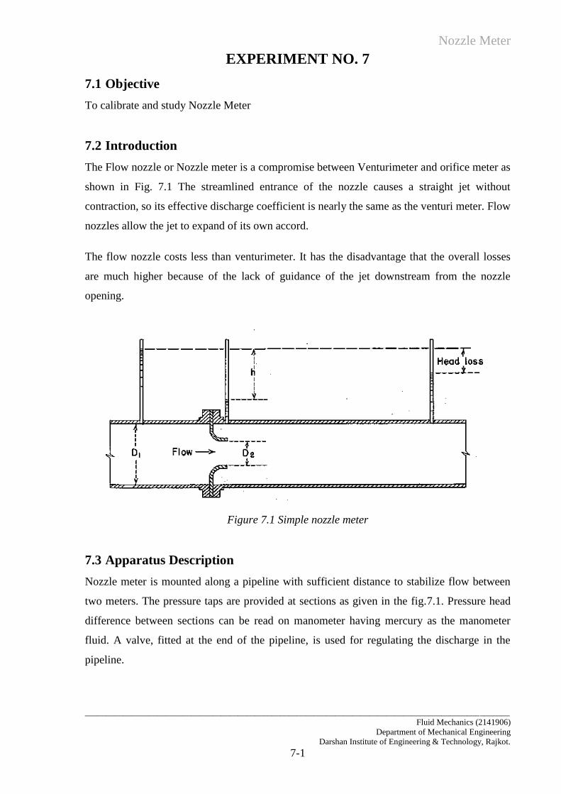
7.2 Introduction
The Flow nozzle or Nozzle meter is a compromise between Venturimeter and orifice meter as
shown in Fig. 7.1 The streamlined entrance of the nozzle causes a straight jet without
contraction, so its effective discharge coefficient is nearly the same as the venturi meter. Flow
nozzles allow the jet to expand of its own accord.
The flow nozzle costs less than venturimeter. It has the disadvantage that the overall losses
are much higher because of the lack of guidance of the jet downstream from the nozzle
opening.
Figure 7.1 Simple nozzle meter
7.3 Apparatus Description
Nozzle meter is mounted along a pipeline with sufficient distance to stabilize flow between
two meters. The pressure taps are provided at sections as given in the fig.7.1. Pressure head
difference between sections can be read on manometer having mercury as the manometer
fluid. A valve, fitted at the end of the pipeline, is used for regulating the discharge in the
pipeline.
Nozzle Meter
____________________________________________________________________________________________________
Fluid Mechanics (2141906)
Department of Mechanical Engineering
Darshan Institute of Engineering & Technology, Rajkot.
7-2
7.4 Technical Specifications of Nozzle meter
Size = 26 mm
Nozzle Size = 16 mm
7.5 Experimental Procedure
1. Fill the storage tank/sump with the water.
2. Switch on the pump and keep the control valve fully open and close the bypass valve
to have maximum flow rate through the meter.
3. Open control valve of the nozzle meter.
4. Open the vent cocks provided at the top of the manometer to drive out the air from the
manometer limbs and close both of them as soon as water start coming out.
5. Note down the difference of level of mercury in the manometer limbs.
6. Keep the drain valve of the collection tank closed till it’s time to start collecting the
water.
7. Close the drain valve of the collection tank and note down the initial level of the water
in the collection tank.
8. Collect known quantity of water in the collection tank and note down the time
required for the same.
9. Change the flow rate of water through the meter with the help of control valve and
repeat the above procedure.
10. Take about 2-3 readings for different flow rates.
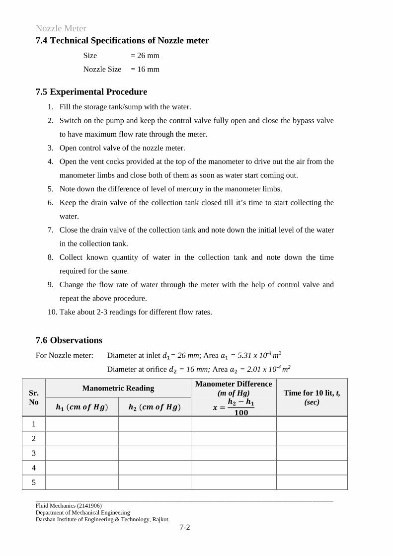
7.6 Observations
For Nozzle meter: Diameter at inlet 𝑑1= 26 mm; Area 𝑎1 = 5.31 x 10⁻⁴ m2
Diameter at orifice 𝑑2 = 16 mm; Area 𝑎2 = 2.01 x 10⁻⁴ m2
Sr.
No
Manometric Reading Manometer Difference
(m of Hg)
𝒙 =𝒉𝟐 − 𝒉𝟏
𝟏𝟎𝟎
Time for 10 lit, t,
(sec) 𝒉𝟏 (𝒄𝒎 𝒐𝒇 𝑯𝒈) 𝒉𝟐 (𝒄𝒎 𝒐𝒇 𝑯𝒈)
1
2
3
4
5
Nozzle Meter
____________________________________________________________________________________________________
Fluid Mechanics (2141906)
Department of Mechanical Engineering
Darshan Institute of Engineering & Technology, Rajkot.
7-3
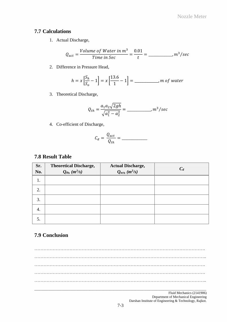
7.7 Calculations
1. Actual Discharge,
𝑄𝑎𝑐𝑡 =𝑉𝑜𝑙𝑢𝑚𝑒 𝑜𝑓 𝑊𝑎𝑡𝑒𝑟 𝑖𝑛 𝑚3
𝑇𝑖𝑚𝑒 𝑖𝑛 𝑆𝑒𝑐=
0.01
𝑡= ______________, 𝑚3 𝑠𝑒𝑐⁄
2. Difference in Pressure Head,
ℎ = 𝑥 [𝑆ℎ
𝑆𝑜− 1] = 𝑥 [
13.6
1− 1] = ______________, 𝑚 𝑜𝑓 𝑤𝑎𝑡𝑒𝑟
3. Theoretical Discharge,
𝑄𝑡ℎ =𝑎1𝑎2√2𝑔ℎ
√𝑎12 − 𝑎2
2= ______________, 𝑚3 𝑠𝑒𝑐⁄
4. Co-efficient of Discharge,
𝐶𝑑 = 𝑄𝑎𝑐𝑡
𝑄𝑡ℎ= _______________
7.8 Result Table
Sr.
No.
Theoretical Discharge,
Qth, (m3/s)
Actual Discharge,
Qact, (m3/s) Cd
1.
2.
3.
4.
5.
7.9 Conclusion
………………………………………………………………………………………………….
…………………………………………………………………………………………………..
………………………………………………………………………………………………….
………………………………………………………………………………………………….
…………………………………………………………………………………………………..

Rota meter
____________________________________________________________________________________________________
Fluid Mechanics (2141906)
Department of Mechanical Engineering
Darshan Institute of Engineering & Technology, Rajkot.
8-1
EXPERIMENT NO. 8
8.1 Objective
To calibrate and study Rotameter
8.2 Introduction
The rotameter is an industrial flow meter used to measure the flow rate of liquids and gases.
The rotameter consists of a tube and float. The float response to flow rate changes is linear.
The rotameter is popular because it has a linear scale, a relatively long measurement range,
and low pressure drop. It is simple to install and maintain.
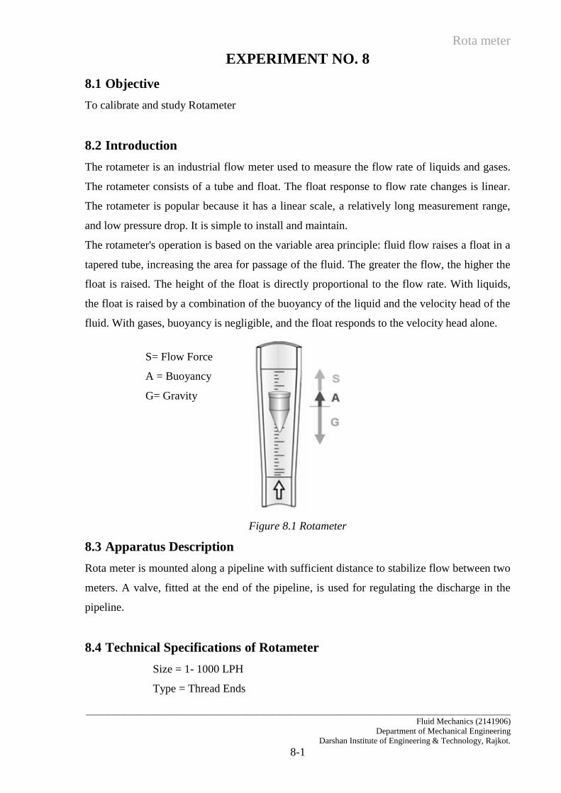
The rotameter's operation is based on the variable area principle: fluid flow raises a float in a
tapered tube, increasing the area for passage of the fluid. The greater the flow, the higher the
float is raised. The height of the float is directly proportional to the flow rate. With liquids,
the float is raised by a combination of the buoyancy of the liquid and the velocity head of the
fluid. With gases, buoyancy is negligible, and the float responds to the velocity head alone.
Figure 8.1 Rotameter
8.3 Apparatus Description
Rota meter is mounted along a pipeline with sufficient distance to stabilize flow between two
meters. A valve, fitted at the end of the pipeline, is used for regulating the discharge in the
pipeline.
8.4 Technical Specifications of Rotameter
Size = 1- 1000 LPH
Type = Thread Ends
S= Flow Force
A = Buoyancy
G= Gravity
Force
Rota meter
____________________________________________________________________________________________________
Fluid Mechanics (2141906)
Department of Mechanical Engineering
Darshan Institute of Engineering & Technology, Rajkot.
8-2
8.5 Experimental Procedure
1. Fill the storage tank/sump with the water.
2. Switch on the pump and keep the control valve fully open and close the bypass valve
to have maximum flow rate through the meter.
3. Verify the rotameter readings flow marking provided by manufacturer.
4. Take about 2-3 readings for different flow rates.
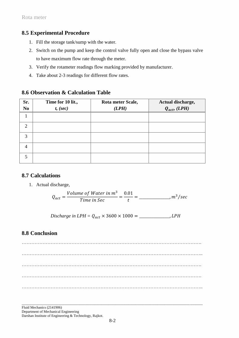
8.6 Observation & Calculation Table
Sr.
No
Time for 10 lit.,
t, (sec)
Rota meter Scale,
(LPH)
Actual discharge,
𝑸𝒂𝒄𝒕, (LPH)
1
2
3
4
5
8.7 Calculations
1. Actual discharge,
𝑄𝑎𝑐𝑡 =𝑉𝑜𝑙𝑢𝑚𝑒 𝑜𝑓 𝑊𝑎𝑡𝑒𝑟 𝑖𝑛 𝑚3
𝑇𝑖𝑚𝑒 𝑖𝑛 𝑆𝑒𝑐=
0.01
𝑡= _________________, 𝑚3 𝑠𝑒𝑐⁄
Discharge in LPH = 𝑄𝑎𝑐𝑡 × 3600 × 1000 = _________________, 𝐿𝑃𝐻
8.8 Conclusion
………………………………………………………………………………………………….
…………………………………………………………………………………………………..
………………………………………………………………………………………………….
………………………………………………………………………………………………….
…………………………………………………………………………………………………..
Pipe Friction Losses
____________________________________________________________________________________________________
Fluid Mechanics (2141906)
Department of Mechanical Engineering
Darshan Institute of Engineering & Technology, Rajkot.
9-1
EXPERIMENT NO. 9
9.1 Objective
To determine fluid friction factor for the given pipes.
9.2 Introduction
The flow of liquid through a pipe is resisted by viscous shear stresses within the liquid and
the turbulence that occurs along the internal walls of the pipe, created by the roughness of the
pipe material. This resistance is usually known as pipe friction and is measured is meters
head of the fluid, thus the term head loss is also used to express the resistance to flow.
Many factors affect the head loss in pipes, the viscosity of the fluid being handled, the size of
the pipes, the roughness of the internal surface of the pipes, the changes in elevations within
the system and the length of travel of the fluid.
The resistance through various valves and fittings will also contribute to the overall head loss.
In a well-designed system the resistance through valves and fittings will be of minor
significance to the overall head loss and thus are called Minor losses in fluid flow.
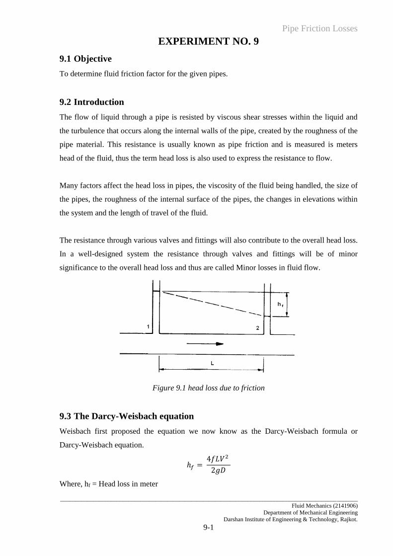
Figure 9.1 head loss due to friction
9.3 The Darcy-Weisbach equation
Weisbach first proposed the equation we now know as the Darcy-Weisbach formula or
Darcy-Weisbach equation.
ℎ𝑓 = 4𝑓𝐿𝑉2
2𝑔𝐷
Where, hf = Head loss in meter
Pipe Friction Losses
____________________________________________________________________________________________________
Fluid Mechanics (2141906)
Department of Mechanical Engineering
Darshan Institute of Engineering & Technology, Rajkot.
9-2
f = Darcy friction factor
L = length of pipe work, (m)
V = Velocity of fluid, (m/sec)
D = inner diameter of pipe, (m)
g = Acceleration due to gravity, (m/sec2)
The Darcy Friction factor used with Weisbach equation has now become the standard head
loss equation for calculating head loss in pipes where the flow is turbulent.
9.4 Apparatus Description
The experimental set up consists of a large number of pipes of different diameters. The pipes
have tapping at certain distance so that a head loss can be measure with the help of a U –
Tube manometer. The flow of water through a pipeline is regulated by operating a control
valve which is provided in main supply line. Actual discharge through pipeline is calculated
by collecting the water in measuring tank and by noting the time for collection.
9.5 Technical Specification
Pipe: MOC = Polyurethane (P.U.)
Test length, L = 1000 mm
Pipe Dia. Pipe 1: Internal Diameter, D1: 16 mm
Pipe 2: Internal Diameter, D2: 21 mm
Pipe 3: Internal Diameter, D3: 26.5 mm
9.6 Experimental Procedure
1. Fill the storage tank/sump with the water.
2. Switch on the pump and keep the control valve fully open and close the bypass valve
to have maximum flow rate through the meter.
3. To find friction factor of pipe 1 open control valve of the same and close other to
valves
4. Open the vent cocks provided for the particular pipe 1 of the manometer.
5. Note down the difference of level of mercury in the manometer limbs.
6. Keep the drain valve of the collection tank open till it’s time to start collecting the
water.
7. Close the drain valve of the collection tank and collect known quantity of water
Pipe Friction Losses
____________________________________________________________________________________________________
Fluid Mechanics (2141906)
Department of Mechanical Engineering
Darshan Institute of Engineering & Technology, Rajkot.
9-3
8. Note down the time required for the same.
9. Change the flow rate of water through the meter with the help of control valve and
repeat the above procedure.
10. Similarly for pipe 2 and 3. Repeat the same procedure indicated in step 4-9
11. Take about 2-3 readings for different flow rates.
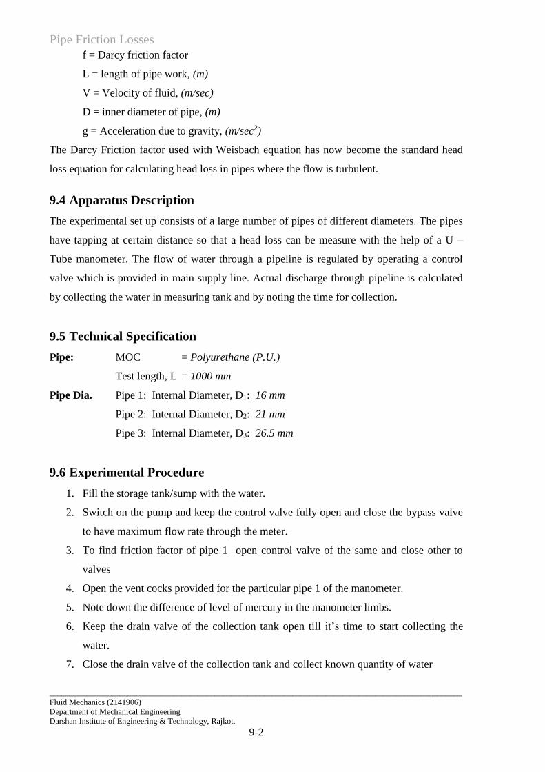
9.7 Observations Table
Length of test section L = 1000 mm = 1 m
Pipe 1 Internal Diameter of Pipe, D1 = 16 mm
Cross Sectional Area of Pipe, A1 = 200.96 mm2 = 2.0 x 10⁻⁴ m2
Sr.
No
Manometric Reading Manometer Difference
(m of Hg)
𝑥 =ℎ2 − ℎ1
100
time for 10 lit, t,
(sec) ℎ1 (𝑐𝑚 𝑜𝑓 𝐻𝑔) ℎ2 (𝑐𝑚 𝑜𝑓 𝐻𝑔)
1
2
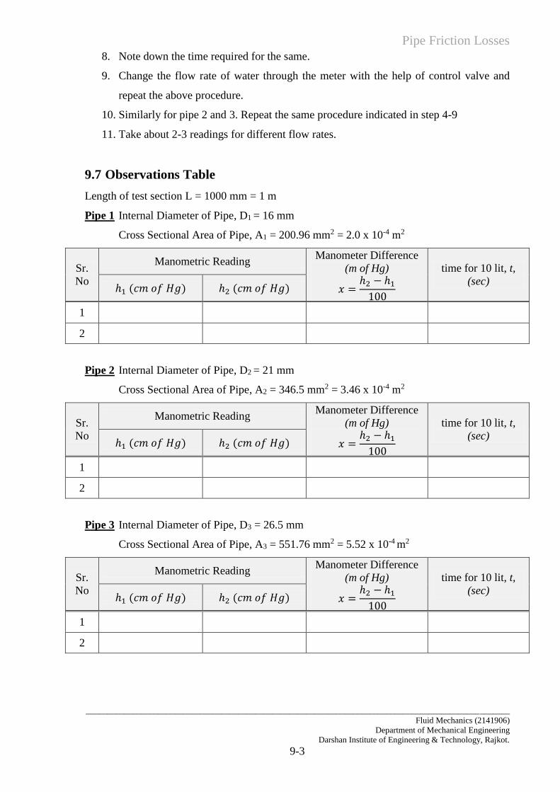
Pipe 2 Internal Diameter of Pipe, D2 = 21 mm
Cross Sectional Area of Pipe, A2 = 346.5 mm2 = 3.46 x 10⁻⁴ m2
Sr.
No
Manometric Reading Manometer Difference
(m of Hg)
𝑥 =ℎ2 − ℎ1
100
time for 10 lit, t,
(sec) ℎ1 (𝑐𝑚 𝑜𝑓 𝐻𝑔) ℎ2 (𝑐𝑚 𝑜𝑓 𝐻𝑔)
1
2
Pipe 3 Internal Diameter of Pipe, D3 = 26.5 mm
Cross Sectional Area of Pipe, A3 = 551.76 mm2 = 5.52 x 10⁻⁴ m2
Sr.
No
Manometric Reading Manometer Difference
(m of Hg)
𝑥 =ℎ2 − ℎ1
100
time for 10 lit, t,
(sec) ℎ1 (𝑐𝑚 𝑜𝑓 𝐻𝑔) ℎ2 (𝑐𝑚 𝑜𝑓 𝐻𝑔)
1
2
Pipe Friction Losses
____________________________________________________________________________________________________
Fluid Mechanics (2141906)
Department of Mechanical Engineering
Darshan Institute of Engineering & Technology, Rajkot.
9-4
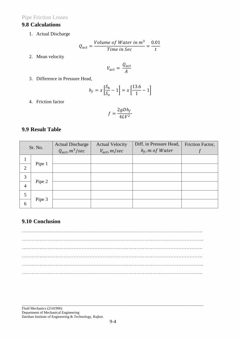
9.8 Calculations
1. Actual Discharge
𝑄𝑎𝑐𝑡 =𝑉𝑜𝑙𝑢𝑚𝑒 𝑜𝑓 𝑊𝑎𝑡𝑒𝑟 𝑖𝑛 𝑚3
𝑇𝑖𝑚𝑒 𝑖𝑛 𝑆𝑒𝑐=
0.01
𝑡
2. Mean velocity
𝑉𝑎𝑐𝑡 = 𝑄𝑎𝑐𝑡
𝐴
3. Difference in Pressure Head,
ℎ𝑓 = 𝑥 [𝑆ℎ
𝑆𝑜− 1] = 𝑥 [
13.6
1− 1]
4. Friction factor
𝑓 =2𝑔𝐷ℎ𝑓
4𝐿𝑉2
9.9 Result Table
Sr. No. Actual Discharge
𝑄𝑎𝑐𝑡, 𝑚3/𝑠𝑒𝑐
Actual Velocity
𝑉𝑎𝑐𝑡, 𝑚/𝑠𝑒𝑐
Diff. in Pressure Head,
ℎ𝑓 , 𝑚 𝑜𝑓 𝑊𝑎𝑡𝑒𝑟
Friction Factor,
f
1 Pipe 1
2
3 Pipe 2
4
5 Pipe 3
6
9.10 Conclusion
………………………………………………………………………………………………….
…………………………………………………………………………………………………..
………………………………………………………………………………………………….
………………………………………………………………………………………………….
…………………………………………………………………………………………………..
………………………………………………………………………………………………….
Minor Losses
____________________________________________________________________________________________________
Fluid Mechanics (2141906)
Department of Mechanical Engineering
Darshan Institute of Engineering & Technology, Rajkot.
10-1
EXPERIMENT NO. 10
10.1 Objective
To determine loss coefficients for different pipe fittings.
10.2 Introduction
While installing a pipeline for conveying a fluid, it is generally not possible to install a long
pipeline of same size all over a straight for various reasons, like space restrictions, aesthetics,
location of outlet etc. Hence, the pipe size varies and it also changes its direction. Also,
various fittings are required to be used. All these variations of sizes and the fittings cause the
loss of fluid head.
Losses due to change in cross-section, bends, elbows, valves and fittings of all types fall into
the category of minor losses in pipelines. In long pipeline, the friction losses are much larger
than these minor losses and hence, the latter are often neglected. But, in shorter pipelines,
their consideration is necessary for the correct estimate of losses.
The minor loses are, generally expressed as
HL = KL (V2
2g)
Where, HL is the minor loss (i.e. head loss)
KL, the loss coefficient, V is the velocity of flow in the pipe
10.3 Apparatus Description
The experimental set-up consists of a pipe of diameter about 24.3 mm fitted with
1. A right angle bend
2. An elbow
3. A Gate Valve
4. A sudden expansion (larger pipe having diameter of about 24.3 mm) and
5. A sudden contraction (from about 24.3 mm to about 13.8 mm)
Sufficient length of the pipeline is provided between various pipe fittings. The pressure taps
on either side of these fittings are suitably provided and the same may be connected to a multi
tube manometer bank. Supply to the line is made through a storage tank and discharge is
regulated by means of outlet valve provided near the outlet end.
Minor Loss
____________________________________________________________________________________________________
Fluid Mechanics (2141906)
Department of Mechanical Engineering
Darshan Institute of Engineering & Technology, Rajkot.
10-2
10.4 Experimental Procedure
1. Fill up sufficient clean water in the sump tank
2. Fill up mercury in the manometer
3. Connect the electric supply. See that the flow control valve and bypass valve are fully
open and all the manometer cocks are closed. Keep the water collecting funnel in the
sump tank side
4. Start the pump and adjust the flow rate. Now slowly open the manometer tapping
connection of small bend. Open both the cocks simultaneously
5. Open air vent cocks. Remove air bubbles and slowly & simultaneously close the
cocks. Note down the manometer reading and flow rate.
6. Close the cocks and similarly, note down the readings for other fittings. Repeat the
procedure for different flow rates.
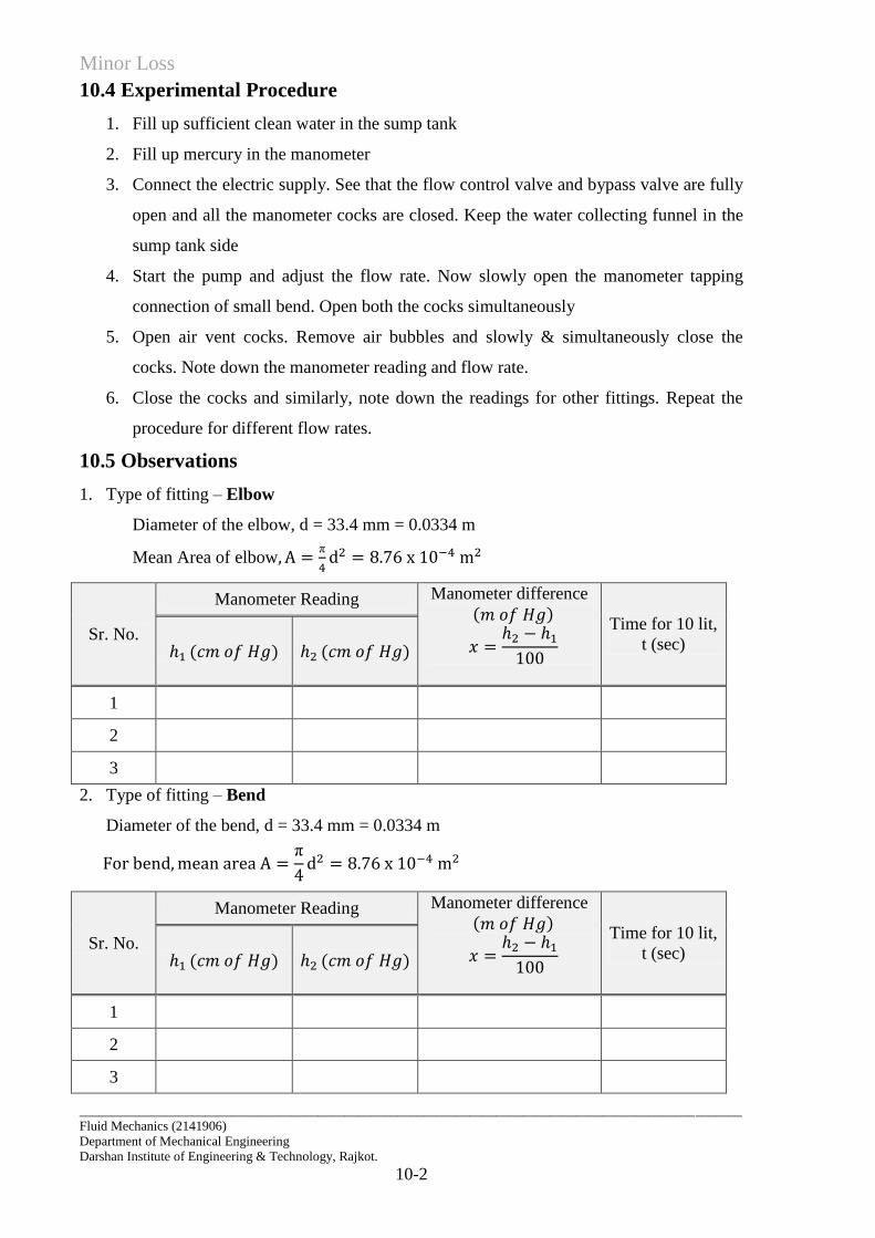
10.5 Observations
1. Type of fitting – Elbow
Diameter of the elbow, d = 33.4 mm = 0.0334 m
Mean Area of elbow, A =π
4d2 = 8.76 x 10⁻⁴ m2
Sr. No.
Manometer Reading Manometer difference
(𝑚 𝑜𝑓 𝐻𝑔)
𝑥 =ℎ2 − ℎ1
100
Time for 10 lit,
t (sec) ℎ1 (𝑐𝑚 𝑜𝑓 𝐻𝑔) ℎ2 (𝑐𝑚 𝑜𝑓 𝐻𝑔)
1
2
3
2. Type of fitting – Bend
Diameter of the bend, d = 33.4 mm = 0.0334 m
For bend, mean area A =π
4d2 = 8.76 x 10⁻⁴ m2
Sr. No.
Manometer Reading Manometer difference
(𝑚 𝑜𝑓 𝐻𝑔)
𝑥 =ℎ2 − ℎ1
100
Time for 10 lit,
t (sec) ℎ1 (𝑐𝑚 𝑜𝑓 𝐻𝑔) ℎ2 (𝑐𝑚 𝑜𝑓 𝐻𝑔)
1
2
3
Minor Losses
____________________________________________________________________________________________________
Fluid Mechanics (2141906)
Department of Mechanical Engineering
Darshan Institute of Engineering & Technology, Rajkot.
10-3
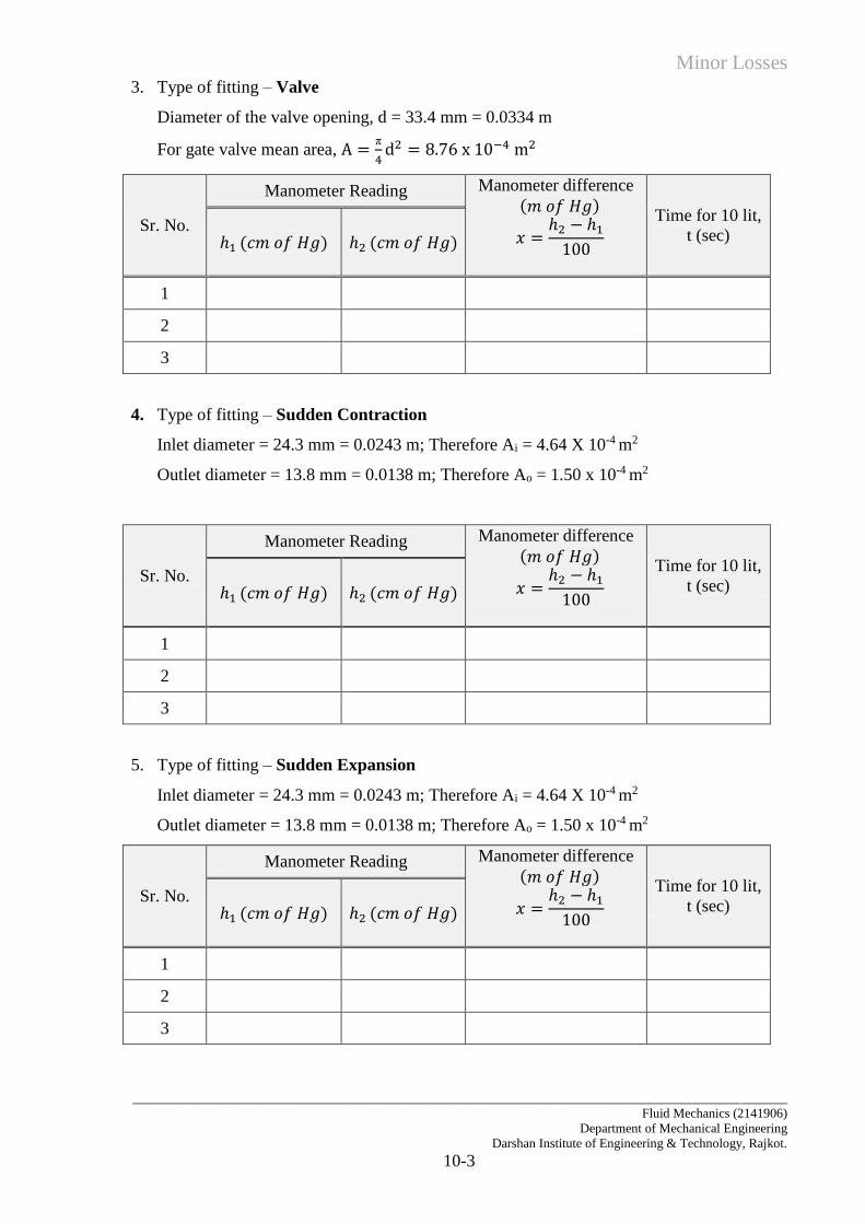
3. Type of fitting – Valve
Diameter of the valve opening, d = 33.4 mm = 0.0334 m
For gate valve mean area, A =π
4d2 = 8.76 x 10⁻⁴ m2
Sr. No.
Manometer Reading Manometer difference
(𝑚 𝑜𝑓 𝐻𝑔)
𝑥 =ℎ2 − ℎ1
100
Time for 10 lit,
t (sec) ℎ1 (𝑐𝑚 𝑜𝑓 𝐻𝑔) ℎ2 (𝑐𝑚 𝑜𝑓 𝐻𝑔)
1
2
3
4. Type of fitting – Sudden Contraction
Inlet diameter = 24.3 mm = 0.0243 m; Therefore Ai = 4.64 X 10⁻⁴ m2
Outlet diameter = 13.8 mm = 0.0138 m; Therefore Ao = 1.50 x 10⁻⁴ m2
Sr. No.
Manometer Reading Manometer difference
(𝑚 𝑜𝑓 𝐻𝑔)
𝑥 =ℎ2 − ℎ1
100
Time for 10 lit,
t (sec) ℎ1 (𝑐𝑚 𝑜𝑓 𝐻𝑔) ℎ2 (𝑐𝑚 𝑜𝑓 𝐻𝑔)
1
2
3
5. Type of fitting – Sudden Expansion
Inlet diameter = 24.3 mm = 0.0243 m; Therefore Ai = 4.64 X 10⁻⁴ m2
Outlet diameter = 13.8 mm = 0.0138 m; Therefore Ao = 1.50 x 10⁻⁴ m2
Sr. No.
Manometer Reading Manometer difference
(𝑚 𝑜𝑓 𝐻𝑔)
𝑥 =ℎ2 − ℎ1
100
Time for 10 lit,
t (sec) ℎ1 (𝑐𝑚 𝑜𝑓 𝐻𝑔) ℎ2 (𝑐𝑚 𝑜𝑓 𝐻𝑔)
1
2
3
Minor Loss
____________________________________________________________________________________________________
Fluid Mechanics (2141906)
Department of Mechanical Engineering
Darshan Institute of Engineering & Technology, Rajkot.
10-4
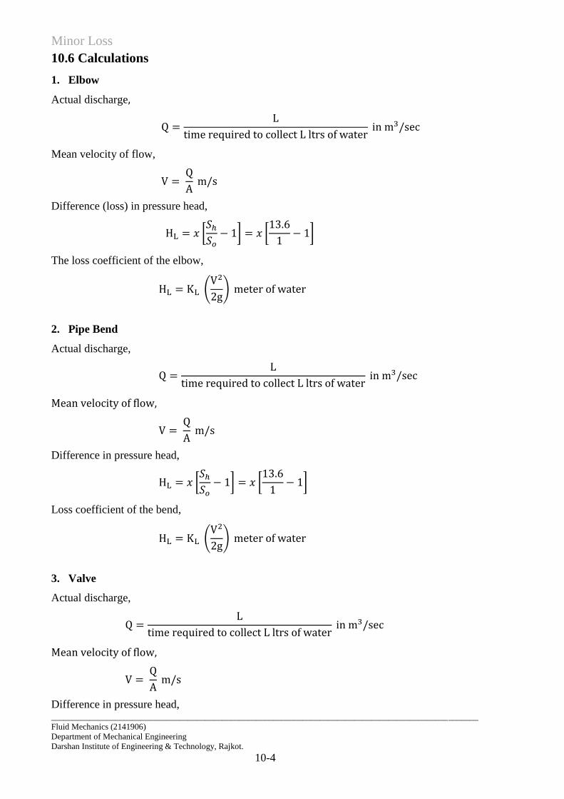
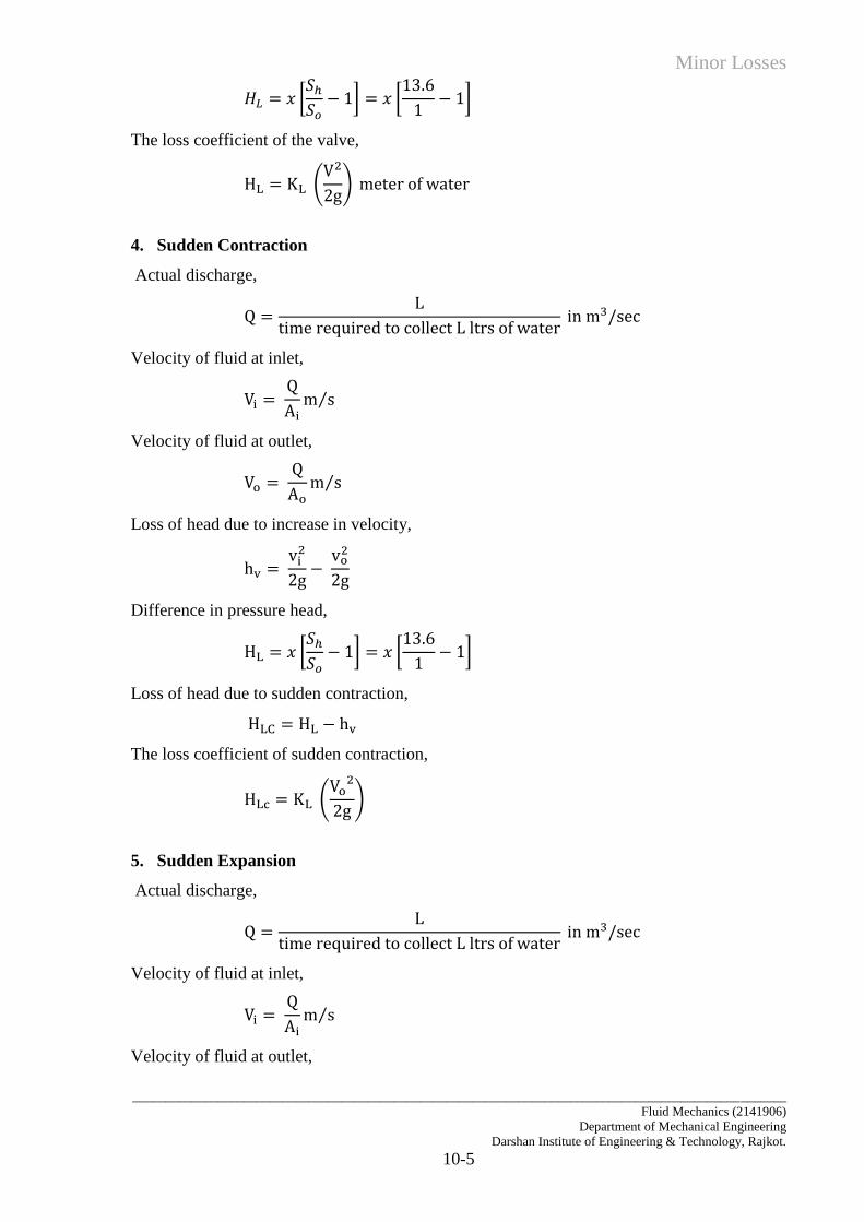
10.6 Calculations
1. Elbow
Actual discharge,
Q =L
time required to collect L ltrs of water in m3/sec
Mean velocity of flow,
V = Q
A m/s
Difference (loss) in pressure head,
HL = 𝑥 [𝑆ℎ
𝑆𝑜− 1] = 𝑥 [
13.6
1− 1]
The loss coefficient of the elbow,
HL = KL (V2
2g) meter of water
2. Pipe Bend
Actual discharge,
Q =L
time required to collect L ltrs of water in m3/sec
Mean velocity of flow,
V = Q
A m/s
Difference in pressure head,
HL = 𝑥 [𝑆ℎ
𝑆𝑜− 1] = 𝑥 [
13.6
1− 1]
Loss coefficient of the bend,
HL = KL (V2
2g) meter of water
3. Valve
Actual discharge,
Q =L
time required to collect L ltrs of water in m3/sec
Mean velocity of flow,
V = Q
A m/s
Difference in pressure head,
Minor Losses
____________________________________________________________________________________________________
Fluid Mechanics (2141906)
Department of Mechanical Engineering
Darshan Institute of Engineering & Technology, Rajkot.
10-5
𝐻𝐿 = 𝑥 [𝑆ℎ
𝑆𝑜− 1] = 𝑥 [
13.6
1− 1]
The loss coefficient of the valve,
HL = KL (V2
2g) meter of water
4. Sudden Contraction
Actual discharge,
Q =L
time required to collect L ltrs of water in m3/sec
Velocity of fluid at inlet,
Vi = Q
Aim s⁄
Velocity of fluid at outlet,
Vo = Q
Aom s⁄
Loss of head due to increase in velocity,
hv = vi
2
2g−
vo2
2g
Difference in pressure head,
HL = 𝑥 [𝑆ℎ
𝑆𝑜− 1] = 𝑥 [
13.6
1− 1]
Loss of head due to sudden contraction,
HLC = HL − hv
The loss coefficient of sudden contraction,
HLc = KL (Vo
2
2g)
5. Sudden Expansion
Actual discharge,
Q =L
time required to collect L ltrs of water in m3/sec
Velocity of fluid at inlet,
Vi = Q
Aim s⁄
Velocity of fluid at outlet,
Minor Loss
____________________________________________________________________________________________________
Fluid Mechanics (2141906)
Department of Mechanical Engineering
Darshan Institute of Engineering & Technology, Rajkot.
10-6
Vo = Q
Aom s⁄
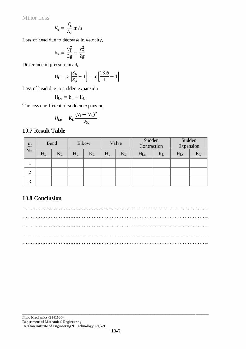
Loss of head due to decrease in velocity,
hv = vi
2
2g−
vo2
2g
Difference in pressure head,
HL = 𝑥 [𝑆ℎ
𝑆𝑜− 1] = 𝑥 [
13.6
1− 1]
Loss of head due to sudden expansion
HLe = hv − HL
The loss coefficient of sudden expansion,
𝐻Le = KL
(Vi − Vo)2
2g
10.7 Result Table
Sr
No.
Bend Elbow Valve Sudden
Contraction
Sudden
Expansion
HL KL HL KL HL KL HLc KL HLe KL
1
2
3
10.8 Conclusion
…………………………………………………………………………………………………..
…………………………………………………………………………………………………..
…………………………………………………………………………………………………..
…………………………………………………………………………………………………..
…………………………………………………………………………………………………..
Pressure Measurement
____________________________________________________________________________________________________
Fluid Mechanics (2141906)
Department of Mechanical Engineering
Darshan Institute of Engineering & Technology, Rajkot.
11-1
EXPERIMENT NO. 11
11.1 Objective
To study pressure and pressure measurement devices.
11.2 Introduction
Fluid pressure can be defined as the measure of force per-unit-area exerted by a fluid, acting
perpendicularly to any surface it contacts The standard SI unit for pressure measurement is
the Pascal (Pa) which is equivalent to one Newton per square meter (N/m2) or the Kilopascal
(kPa) where 1 kPa = 1000 Pa.
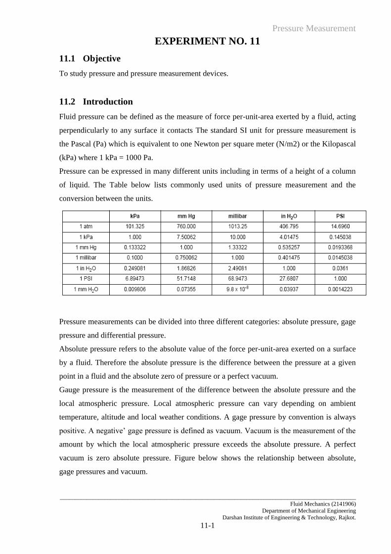
Pressure can be expressed in many different units including in terms of a height of a column
of liquid. The Table below lists commonly used units of pressure measurement and the
conversion between the units.
Pressure measurements can be divided into three different categories: absolute pressure, gage
pressure and differential pressure.
Absolute pressure refers to the absolute value of the force per-unit-area exerted on a surface
by a fluid. Therefore the absolute pressure is the difference between the pressure at a given
point in a fluid and the absolute zero of pressure or a perfect vacuum.
Gauge pressure is the measurement of the difference between the absolute pressure and the
local atmospheric pressure. Local atmospheric pressure can vary depending on ambient
temperature, altitude and local weather conditions. A gage pressure by convention is always
positive. A negative’ gage pressure is defined as vacuum. Vacuum is the measurement of the
amount by which the local atmospheric pressure exceeds the absolute pressure. A perfect
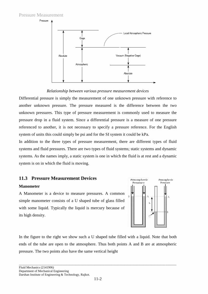
vacuum is zero absolute pressure. Figure below shows the relationship between absolute,
gage pressures and vacuum.
Pressure Measurement
____________________________________________________________________________________________________
Fluid Mechanics (2141906)
Department of Mechanical Engineering
Darshan Institute of Engineering & Technology, Rajkot.
11-2
Relationship between various pressure measurement devices
Differential pressure is simply the measurement of one unknown pressure with reference to
another unknown pressure. The pressure measured is the difference between the two
unknown pressures. This type of pressure measurement is commonly used to measure the
pressure drop in a fluid system. Since a differential pressure is a measure of one pressure
referenced to another, it is not necessary to specify a pressure reference. For the English
system of units this could simply be psi and for the SI system it could be kPa.
In addition to the three types of pressure measurement, there are different types of fluid
systems and fluid pressures. There are two types of fluid systems; static systems and dynamic
systems. As the names imply, a static system is one in which the fluid is at rest and a dynamic
system is on in which the fluid is moving.
11.3 Pressure Measurement Devices
Manometer
A Manometer is a device to measure pressures. A common
simple manometer consists of a U shaped tube of glass filled
with some liquid. Typically the liquid is mercury because of
its high density.
In the figure to the right we show such a U shaped tube filled with a liquid. Note that both
ends of the tube are open to the atmosphere. Thus both points A and B are at atmospheric
pressure. The two points also have the same vertical height
Pressure Measurement
____________________________________________________________________________________________________
Fluid Mechanics (2141906)
Department of Mechanical Engineering
Darshan Institute of Engineering & Technology, Rajkot.
11-3
Now the top of the tube on the left has been closed. We imagine that there is a sample of gas
in the closed end of the tube. The right side of the tube remains open to the atmosphere. The
point A, then, is at atmospheric pressure.
The point C is at the pressure of the gas in the closed end of the tube. The point B has a
pressure greater than atmospheric pressure due to the weight of the column of liquid of height
h. The point C is at the same height as B, so it has the same pressure as B. And this is equal to
the pressure of the gas in the closed end of the tube. Thus, in this case the pressure of the gas
that is trapped in the closed end of the tube is greater than atmospheric pressure by the
amount of pressure exerted by the column of liquid of height h.
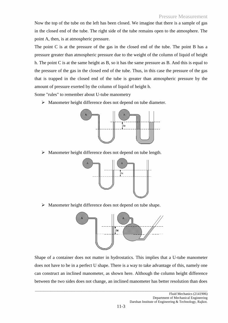
Some "rules" to remember about U-tube manometry
Manometer height difference does not depend on tube diameter.
Manometer height difference does not depend on tube length.
Manometer height difference does not depend on tube shape.
Shape of a container does not matter in hydrostatics. This implies that a U-tube manometer
does not have to be in a perfect U shape. There is a way to take advantage of this, namely one
can construct an inclined manometer, as shown here. Although the column height difference
between the two sides does not change, an inclined manometer has better resolution than does
Pressure Measurement
____________________________________________________________________________________________________
Fluid Mechanics (2141906)
Department of Mechanical Engineering
Darshan Institute of Engineering & Technology, Rajkot.
11-4
a standard vertical manometer because of the inclined right side. Specifically, for a given
ruler resolution, one "tick" mark on the ruler corresponds to a finer gradation of pressure for
the inclined case.
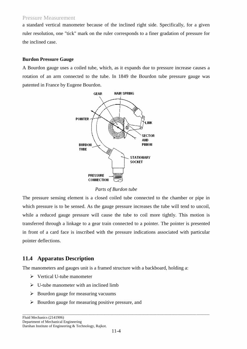
Burdon Pressure Gauge
A Bourdon gauge uses a coiled tube, which, as it expands due to pressure increase causes a
rotation of an arm connected to the tube. In 1849 the Bourdon tube pressure gauge was
patented in France by Eugene Bourdon.
Parts of Burdon tube
The pressure sensing element is a closed coiled tube connected to the chamber or pipe in
which pressure is to be sensed. As the gauge pressure increases the tube will tend to uncoil,
while a reduced gauge pressure will cause the tube to coil more tightly. This motion is
transferred through a linkage to a gear train connected to a pointer. The pointer is presented
in front of a card face is inscribed with the pressure indications associated with particular
pointer deflections.
11.4 Apparatus Description
The manometers and gauges unit is a framed structure with a backboard, holding a:
Vertical U-tube manometer
U-tube manometer with an inclined limb
Bourdon gauge for measuring vacuums
Bourdon gauge for measuring positive pressure, and
Pressure Measurement
____________________________________________________________________________________________________
Fluid Mechanics (2141906)
Department of Mechanical Engineering
Darshan Institute of Engineering & Technology, Rajkot.
11-5
Syringe assembly for pressurizing and reducing pressure in the measurement devices.
Each gauge and manometer has a delivery point to connect to the syringe using plastic tubing
(included). All connections are push-fit, and T-pieces are provided to enable two instruments
to be connected to one point.
11.5 Experimental Procedure
1. Using the syring connects its plastic tubing to Pressure gauge. Push the syring arm to
generate pressure. Observe the deflection on the gauge
2. Now connect the syring tubing to vacuum gauge. Release the arm of syring to
generate vacuum and observe the change in deflection.
3. U tube Manometer can be connected to any of the flow meter devices. Switch the
pump and observe the change in mercury levels in the manometer. Calculate the
pressure difference.
4. Similarly connect the Inclined U tube manometer to any of the flow meter and
calculate pressure difference
11.6 Observations:
Density of liquid flowing in pipe =
Density of liquid flowing in pipe =
Sr. No. Type of Manometer Manometric Reading
Pressure/Pressure Difference h1 h2
1 U tube Manometer
2 Inclined Tube Manometer
3 Pressure Gauge
4 Vacuum Gauge
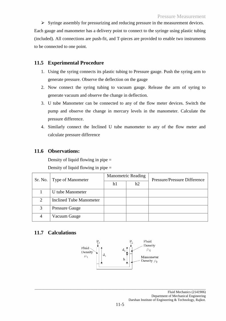
11.7 Calculations
Pressure Measurement
____________________________________________________________________________________________________
Fluid Mechanics (2141906)
Department of Mechanical Engineering
Darshan Institute of Engineering & Technology, Rajkot.
11-6
In the above figure, since the pressure at the height of the lower surface of the manometer
fluid is the same in both arms of the manometer, we can write the following equation:
P1 + ρ1gd1 = P2 + ρ2gd2 + ρf g h
Here, ρ1 = ρ2 = ρw = Density of water;
P1 - P2 = ρwgd2 + ρf g h – ρwgd1
Also d1- d2 = h
P1 - P2 = (ρf - ρw) g h
Here ρf = Density of Mercury;
Substituting Standard Values
P1-P2 = 13580 – 1000 (kg/m3) x g (m/s2) x h/1000 (m) = 12.58 g h (in N/m2)
Where g =9.81 m/s2; h in mm
11.8 Conclusion
………………………………………………………………………………………………….
…………………………………………………………………………………………………..
………………………………………………………………………………………………….
…………………………………………………………………………………………………..
…………………………………………………………………………………………………
Free and Forced Vortex Flow
____________________________________________________________________________________________________
Fluid Mechanics (2141906)
Department of Mechanical Engineering
Darshan Institute of Engineering & Technology, Rajkot. 12-1
EXPERIMENT NO. 12
12.1 Objective
To obtain surface profile of free and forced vortex flow.
12.2 Introduction
A vortex is a spinning, often turbulent, flow of fluid. Any spiral motion with closed
streamlines is vortex flow. The motion of the fluid swirling rapidly around a center is called a
vortex.
When a liquid contained in a cylindrical vessel is given the rotation surface of water no
longer remains horizontal but it depresses at the centre and rises near the walls of the vessel.
A rotating mass of fluid is called vortex and motion of rotating mass of fluid is vortex
motion. Vortices are of two type viz., forced vortex and free vortex. When a cylinder is in
rotation then a vortex is called forced vortex. If water enters a stationary cylinder then a
vortex is called free vortex.
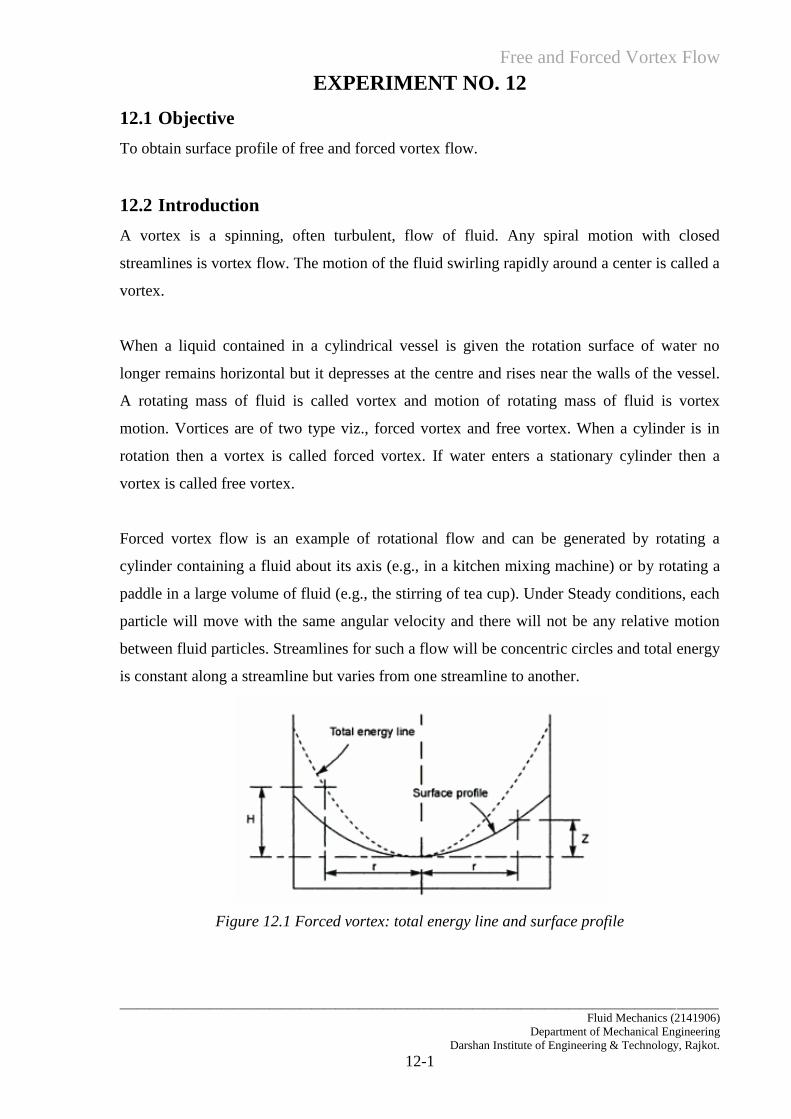
Forced vortex flow is an example of rotational flow and can be generated by rotating a
cylinder containing a fluid about its axis (e.g., in a kitchen mixing machine) or by rotating a
paddle in a large volume of fluid (e.g., the stirring of tea cup). Under Steady conditions, each
particle will move with the same angular velocity and there will not be any relative motion
between fluid particles. Streamlines for such a flow will be concentric circles and total energy
is constant along a streamline but varies from one streamline to another.
Figure 12.1 Forced vortex: total energy line and surface profile
Free and Forced vortex Flow
____________________________________________________________________________________________________
Fluid Mechanics (2141906)
Department of Mechanical Engineering
Darshan Institute of Engineering & Technology, Rajkot. 12- 2
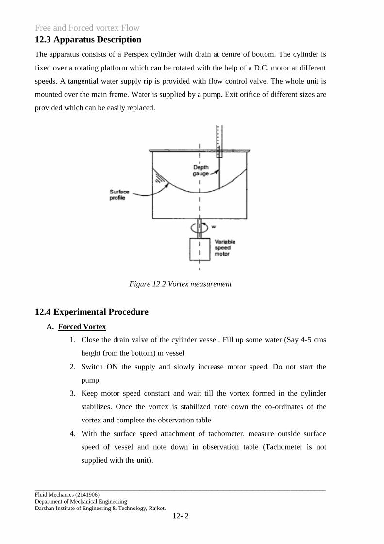
12.3 Apparatus Description
The apparatus consists of a Perspex cylinder with drain at centre of bottom. The cylinder is
fixed over a rotating platform which can be rotated with the help of a D.C. motor at different
speeds. A tangential water supply rip is provided with flow control valve. The whole unit is
mounted over the main frame. Water is supplied by a pump. Exit orifice of different sizes are
provided which can be easily replaced.
Figure 12.2 Vortex measurement
12.4 Experimental Procedure
A. Forced Vortex
1. Close the drain valve of the cylinder vessel. Fill up some water (Say 4-5 cms
height from the bottom) in vessel
2. Switch ON the supply and slowly increase motor speed. Do not start the
pump.
3. Keep motor speed constant and wait till the vortex formed in the cylinder
stabilizes. Once the vortex is stabilized note down the co-ordinates of the
vortex and complete the observation table
4. With the surface speed attachment of tachometer, measure outside surface
speed of vessel and note down in observation table (Tachometer is not
supplied with the unit).
Free and Forced Vortex Flow
____________________________________________________________________________________________________
Fluid Mechanics (2141906)
Department of Mechanical Engineering
Darshan Institute of Engineering & Technology, Rajkot. 12-3
B. Free Vortex
1. Open the bypass valve and start the pump
2. Slowly close the water bypass valve and drain valve of the cylinder. Water is
now getting admitted through the tangential entry pipe to the cylinder
3. Properly adjust the bottom drain valve of vessel so that a stable vortex is
formed
4. Note down co-ordinate of the vortex. Also measure time required for L lit
level rise in measuring tank and complete observation table.
12.5 Observation Table:
A. Forced Vortex
Sr. No. RPM of motor (N”) Radius (X coordinate) cms Height (z) (Y coordinate) cms
1
B. Free Vortex
Sr. No Radius
(X coordinate), cms
Height (z)
(Y coordinate), cms
Time for L=______ lit. level
rise, t (sec)
1
12.6 Calculations
A. Forced Vortex
Free and Forced vortex Flow
____________________________________________________________________________________________________
Fluid Mechanics (2141906)
Department of Mechanical Engineering
Darshan Institute of Engineering & Technology, Rajkot. 12- 4
B. Free Vortex
Pipe diameter, d = 1.6 cm; A=2.01 x 10⁻⁴
m2
(Note- For forced vortex, linear velocity of the cylinder does not equal the actual water
velocity near I.D. of cylinder. Also for free vortex, as water does not enter exactly
tangentially & velocity changes after it enters the cylinder which is not known, it is very
difficult to calculate velocity of water exactly, the theoretical calculations deviate much from
the observations. It can be readily observed that water comes out from pipe with high
velocity, but velocity of water near the walls of cylinder appears to be very less)
12.7 Conclusion
………………………………………………………………………………………………….
…………………………………………………………………………………………………..
………………………………………………………………………………………………….
12.8 Precautions
1. While making the experiment forced vortex, see that water does not spill away from
the vessel. Do not increase the speed of rotation excessively.
2. Do not start pump for forced vortex experiment
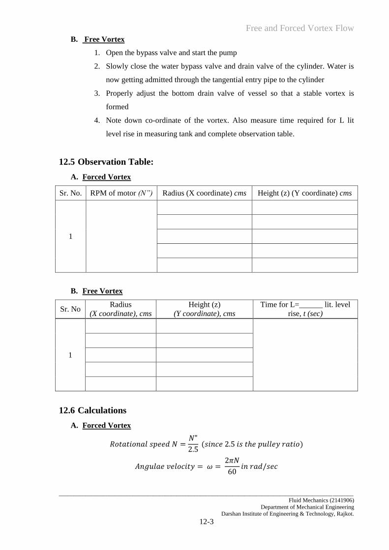
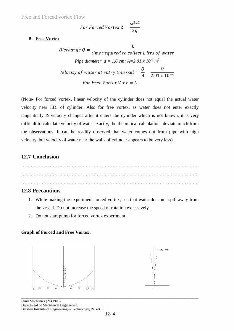
Graph of Forced and Free Vortex:
Reynolds’s Apparatus
____________________________________________________________________________________________________
Fluid Mechanics (2141906)
Department of Mechanical Engineering
Darshan Institute of Engineering & Technology, Rajkot.
13-1
EXPERIMENT NO. 13
13.1 Objective
To study Laminar and Turbulent flow and it’s visualization on Reynolds’s apparatus
13.2 Introduction
The properties of density and specific gravity are measures of the “heaviness” of fluid. These
properties are however not sufficient to uniquely characterize how fluids behave since two
fluids (such as water and oil) can have approximately the same value of density but behaves
quite differently when flowing. There is apparently some additional property that is needed to
describe the “fluidity” of the fluid.
Viscosity is defined as the property of a fluid which offers resistance to the movement of one
layer of fluid over another adjacent layer of the fluid. It is an inherent property of each fluid.
Its effect is similar to the frictional resistance of one body sliding over other body, as
viscosity offers frictional resistance to the motion of the fluid consequently. In order to
maintain the flow, extra energy is to be supplied to overcome effect of viscosity. The
frictional energy generated comes out in form of heat and dissipated to the atmosphere
through boundary surfaces.
13.3 Types of flow
13.3.1 Laminar flow
Laminar flow is that type of flow in which the particle of the fluid moves along well defined
parts or streamlines. In laminar flow all streamlines are straight and parallel. In laminar flow
one layer of fluid is sliding over another layer, whenever the Reynolds number is less than
2000, the flow is said to be laminar. In laminar flow, energy loss is low and it is directly
proportional to the velocity of the fluid. The following reasons are for the laminar flow, fluid
has low velocity, fluid has high viscosity and diameter of pipe is large
13.3.2 Turbulent Flow:
The flow is said to be turbulent flow it he flow moves in a zigzag way. Due to movement of
the particles in a zigzag way, the eddies formation take place which are responsible of high-
energy losses.
Reynolds’s Apparatus
____________________________________________________________________________________________________
Fluid Mechanics (2141906)
Department of Mechanical Engineering
Darshan Institute of Engineering & Technology, Rajkot.
13-2
In turbulent flow, energy loss is directly proportional to the square of velocity of fluid. If
Reynolds number is greater than 4000, then flow is said to be turbulent
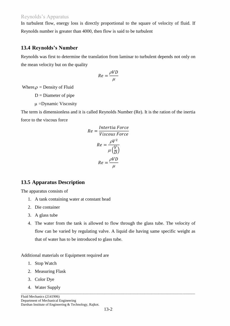
13.4 Reynolds’s Number
Reynolds was first to determine the translation from laminar to turbulent depends not only on
the mean velocity but on the quality
𝑅𝑒 =𝑉𝐷
Where, = Density of Fluid
D = Diameter of pipe
=Dynamic Viscosity
The term is dimensionless and it is called Reynolds Number (Re). It is the ration of the inertia
force to the viscous force
𝑅𝑒 =𝐼𝑛𝑡𝑒𝑟𝑡𝑖𝑎 𝐹𝑜𝑟𝑐𝑒
𝑉𝑖𝑠𝑐𝑜𝑢𝑠 𝐹𝑜𝑟𝑐𝑒
𝑅𝑒 =𝑉2
(𝑉𝐷)
𝑅𝑒 =𝑉𝐷
13.5 Apparatus Description
The apparatus consists of
1. A tank containing water at constant head
2. Die container
3. A glass tube
4. The water from the tank is allowed to flow through the glass tube. The velocity of
flow can be varied by regulating valve. A liquid die having same specific weight as
that of water has to be introduced to glass tube.
Additional materials or Equipment required are
1. Stop Watch
2. Measuring Flask
3. Color Dye
4. Water Supply
Reynolds’s Apparatus
____________________________________________________________________________________________________
Fluid Mechanics (2141906)
Department of Mechanical Engineering
Darshan Institute of Engineering & Technology, Rajkot.
13-3
13.6 Experimental Procedure
1. Switch on the pump and fill the head tank. Manually also fill the dye tank with some
amount of bright dye liquid provided.
2. Open the control valve slowly at the bottom of the tube and release small flow of dye.
3. Observe the flow in the tube.
4. Note down the time for 1 liter of discharge with the help of stopwatch and measuring
flask.
5. Repeat the above process for various discharges
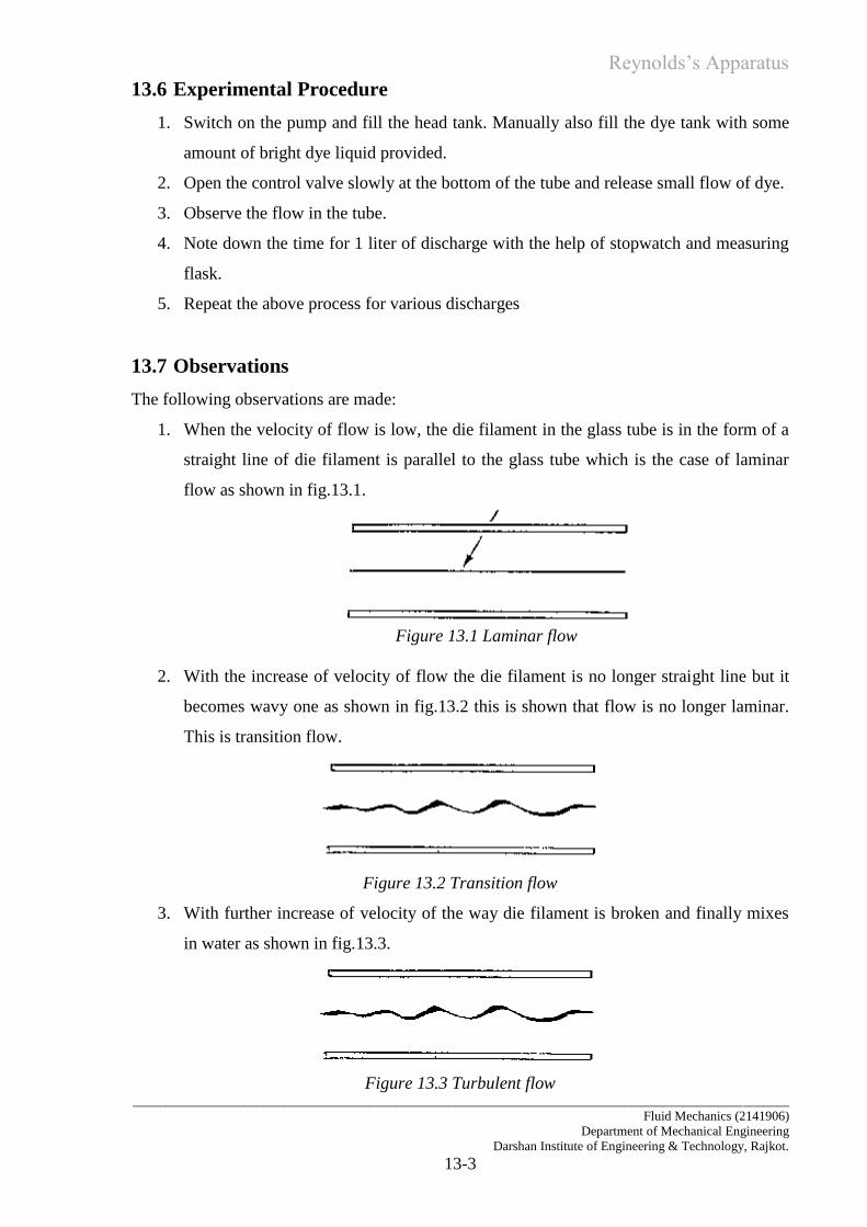
13.7 Observations
The following observations are made:
1. When the velocity of flow is low, the die filament in the glass tube is in the form of a
straight line of die filament is parallel to the glass tube which is the case of laminar
flow as shown in fig.13.1.
Figure 13.1 Laminar flow
2. With the increase of velocity of flow the die filament is no longer straight line but it
becomes wavy one as shown in fig.13.2 this is shown that flow is no longer laminar.
This is transition flow.
Figure 13.2 Transition flow
3. With further increase of velocity of the way die filament is broken and finally mixes
in water as shown in fig.13.3.
Figure 13.3 Turbulent flow
Reynolds’s Apparatus
____________________________________________________________________________________________________
Fluid Mechanics (2141906)
Department of Mechanical Engineering
Darshan Institute of Engineering & Technology, Rajkot.
13-4
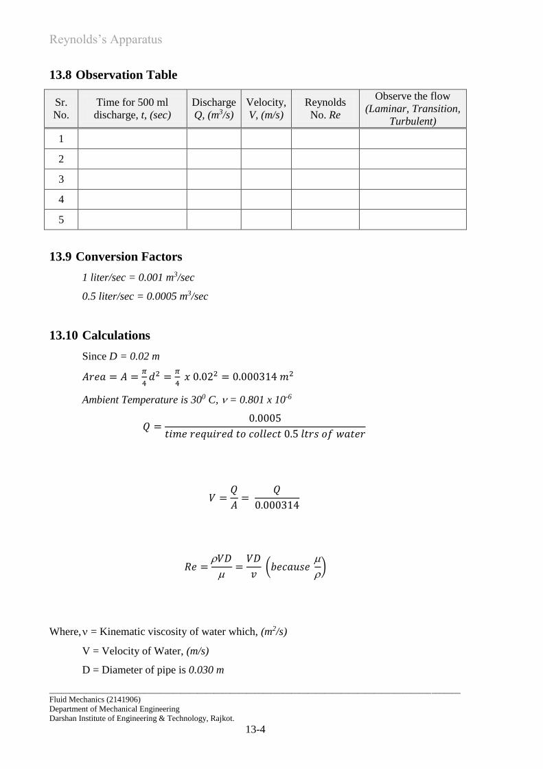
13.8 Observation Table
Sr.
No.
Time for 500 ml
discharge, t, (sec)
Discharge
Q, (m3/s)
Velocity,
V, (m/s)
Reynolds
No. Re
Observe the flow
(Laminar, Transition,
Turbulent)
1
2
3
4
5
13.9 Conversion Factors
1 liter/sec = 0.001 m3/sec
0.5 liter/sec = 0.0005 m3/sec
13.10 Calculations
Since D = 0.02 m
𝐴𝑟𝑒𝑎 = 𝐴 =𝜋
4𝑑2 =
𝜋
4 𝑥 0.022 = 0.000314 𝑚2
Ambient Temperature is 300 C, = 0.801 x 10⁻⁶
𝑄 =0.0005
𝑡𝑖𝑚𝑒 𝑟𝑒𝑞𝑢𝑖𝑟𝑒𝑑 𝑡𝑜 𝑐𝑜𝑙𝑙𝑒𝑐𝑡 0.5 𝑙𝑡𝑟𝑠 𝑜𝑓 𝑤𝑎𝑡𝑒𝑟
𝑉 =𝑄
𝐴=
𝑄
0.000314
𝑅𝑒 =𝑉𝐷
=
𝑉𝐷
𝑣 (𝑏𝑒𝑐𝑎𝑢𝑠𝑒
)
Where, = Kinematic viscosity of water which, (m2/s)
V = Velocity of Water, (m/s)
D = Diameter of pipe is 0.030 m
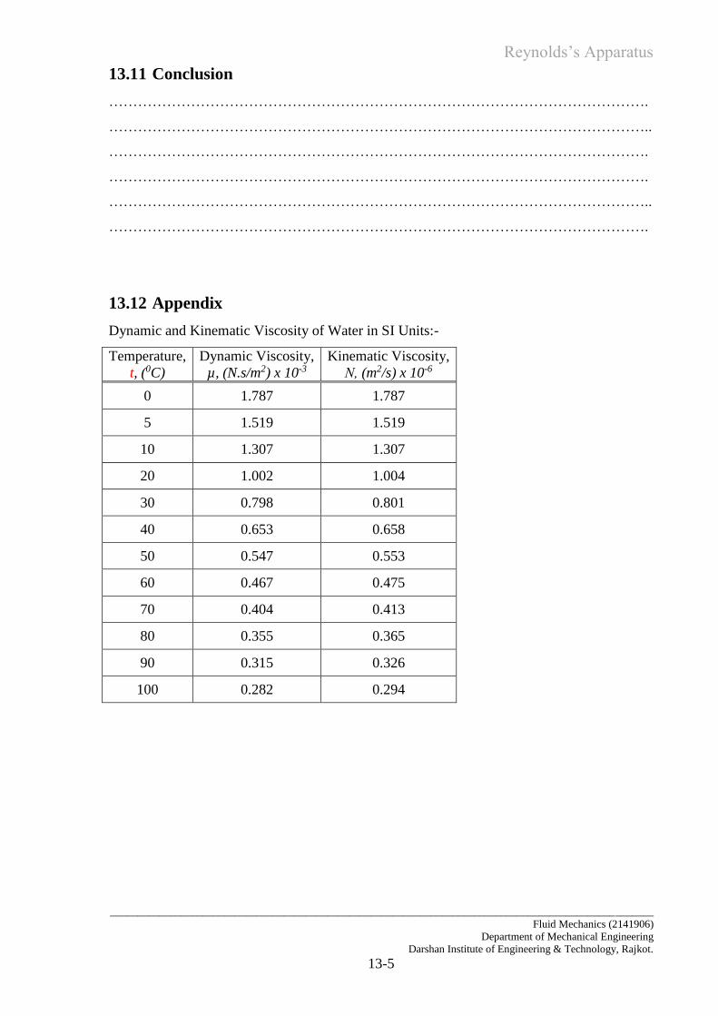
Reynolds’s Apparatus
____________________________________________________________________________________________________
Fluid Mechanics (2141906)
Department of Mechanical Engineering
Darshan Institute of Engineering & Technology, Rajkot.
13-5
13.11 Conclusion
………………………………………………………………………………………………….
…………………………………………………………………………………………………..
………………………………………………………………………………………………….
………………………………………………………………………………………………….
…………………………………………………………………………………………………..
………………………………………………………………………………………………….
13.12 Appendix
Dynamic and Kinematic Viscosity of Water in SI Units:-
Temperature,
t, (0C)
Dynamic Viscosity,
µ, (N.s/m2) x 10-3
Kinematic Viscosity,
Ν, (m2/s) x 10-6
0 1.787 1.787
5 1.519 1.519
10 1.307 1.307
20 1.002 1.004
30 0.798 0.801
40 0.653 0.658
50 0.547 0.553
60 0.467 0.475
70 0.404 0.413
80 0.355 0.365
90 0.315 0.326
100 0.282 0.294

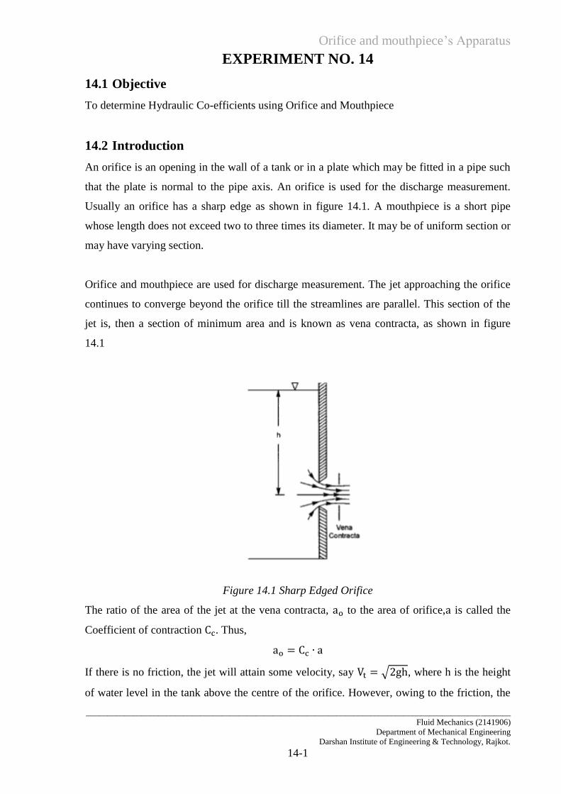
Orifice and mouthpiece’s Apparatus
____________________________________________________________________________________________________
Fluid Mechanics (2141906)
Department of Mechanical Engineering
Darshan Institute of Engineering & Technology, Rajkot.
14-1
EXPERIMENT NO. 14
14.1 Objective
To determine Hydraulic Co-efficients using Orifice and Mouthpiece
14.2 Introduction
An orifice is an opening in the wall of a tank or in a plate which may be fitted in a pipe such
that the plate is normal to the pipe axis. An orifice is used for the discharge measurement.
Usually an orifice has a sharp edge as shown in figure 14.1. A mouthpiece is a short pipe
whose length does not exceed two to three times its diameter. It may be of uniform section or
may have varying section.
Orifice and mouthpiece are used for discharge measurement. The jet approaching the orifice
continues to converge beyond the orifice till the streamlines are parallel. This section of the
jet is, then a section of minimum area and is known as vena contracta, as shown in figure
14.1
Figure 14.1 Sharp Edged Orifice
The ratio of the area of the jet at the vena contracta, to the area of orifice, is called the
Coefficient of contraction . Thus,
If there is no friction, the jet will attain some velocity, say √ , where h is the height
of water level in the tank above the centre of the orifice. However, owing to the friction, the
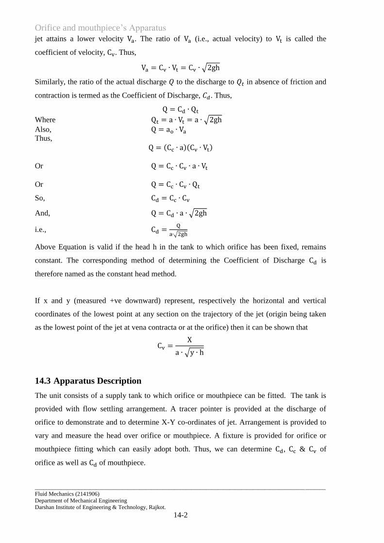
Orifice and mouthpiece’s Apparatus
____________________________________________________________________________________________________
Fluid Mechanics (2141906)
Department of Mechanical Engineering
Darshan Institute of Engineering & Technology, Rajkot.
14-2
jet attains a lower velocity . The ratio of (i.e., actual velocity) to is called the
coefficient of velocity, . Thus,
√
Similarly, the ratio of the actual discharge to the discharge to in absence of friction and
contraction is termed as the Coefficient of Discharge, . Thus,
Where √ Also, Thus,
( )( ) Or Or
So,
And, √
i.e.,
√
Above Equation is valid if the head h in the tank to which orifice has been fixed, remains
constant. The corresponding method of determining the Coefficient of Discharge is
therefore named as the constant head method.
If x and y (measured +ve downward) represent, respectively the horizontal and vertical
coordinates of the lowest point at any section on the trajectory of the jet (origin being taken
as the lowest point of the jet at vena contracta or at the orifice) then it can be shown that
√
14.3 Apparatus Description
The unit consists of a supply tank to which orifice or mouthpiece can be fitted. The tank is
provided with flow settling arrangement. A tracer pointer is provided at the discharge of
orifice to demonstrate and to determine X-Y co-ordinates of jet. Arrangement is provided to
vary and measure the head over orifice or mouthpiece. A fixture is provided for orifice or
mouthpiece fitting which can easily adopt both. Thus, we can determine , & of
orifice as well as of mouthpiece.
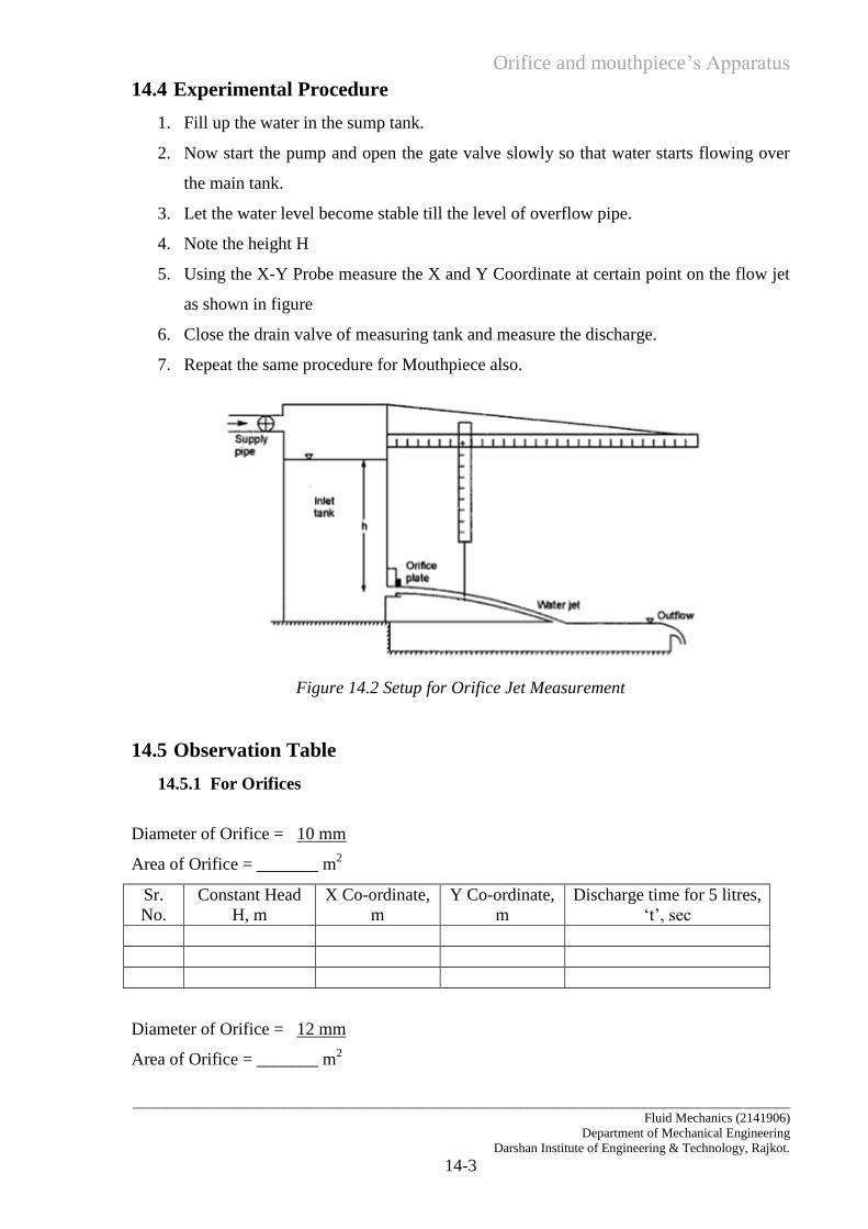
Orifice and mouthpiece’s Apparatus
____________________________________________________________________________________________________
Fluid Mechanics (2141906)
Department of Mechanical Engineering
Darshan Institute of Engineering & Technology, Rajkot.
14-3
14.4 Experimental Procedure
1. Fill up the water in the sump tank.
2. Now start the pump and open the gate valve slowly so that water starts flowing over
the main tank.
3. Let the water level become stable till the level of overflow pipe.
4. Note the height H
5. Using the X-Y Probe measure the X and Y Coordinate at certain point on the flow jet
as shown in figure
6. Close the drain valve of measuring tank and measure the discharge.
7. Repeat the same procedure for Mouthpiece also.
Figure 14.2 Setup for Orifice Jet Measurement
14.5 Observation Table
14.5.1 For Orifices
Diameter of Orifice = 10 mm
Area of Orifice = _______ m2
Sr.
No.
Constant Head
H, m
X Co-ordinate,
m
Y Co-ordinate,
m
Discharge time for 5 litres,
‘t’, sec
Diameter of Orifice = 12 mm
Area of Orifice = _______ m2
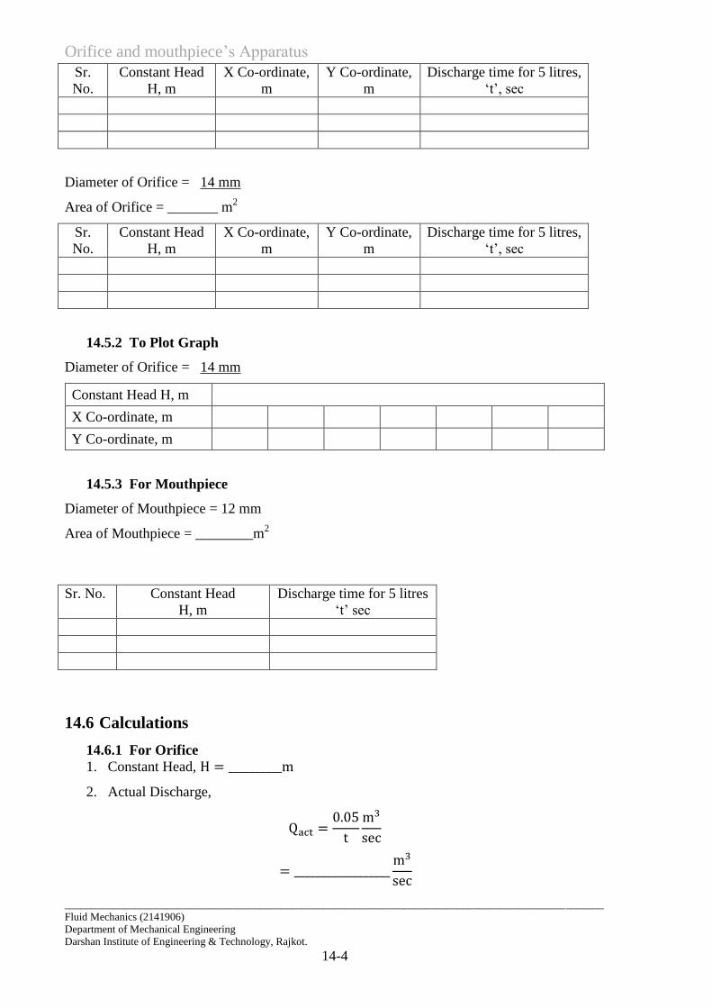
Orifice and mouthpiece’s Apparatus
____________________________________________________________________________________________________
Fluid Mechanics (2141906)
Department of Mechanical Engineering
Darshan Institute of Engineering & Technology, Rajkot.
14-4
Sr.
No.
Constant Head
H, m
X Co-ordinate,
m
Y Co-ordinate,
m
Discharge time for 5 litres,
‘t’, sec
Diameter of Orifice = 14 mm
Area of Orifice = _______ m2
Sr.
No.
Constant Head
H, m
X Co-ordinate,
m
Y Co-ordinate,
m
Discharge time for 5 litres,
‘t’, sec
14.5.2 To Plot Graph
Diameter of Orifice = 14 mm
Constant Head H, m
X Co-ordinate, m
Y Co-ordinate, m
14.5.3 For Mouthpiece
Diameter of Mouthpiece = 12 mm
Area of Mouthpiece = ________m2
Sr. No. Constant Head
H, m
Discharge time for 5 litres
‘t’ sec
14.6 Calculations
14.6.1 For Orifice
1. Constant Head,
2. Actual Discharge,
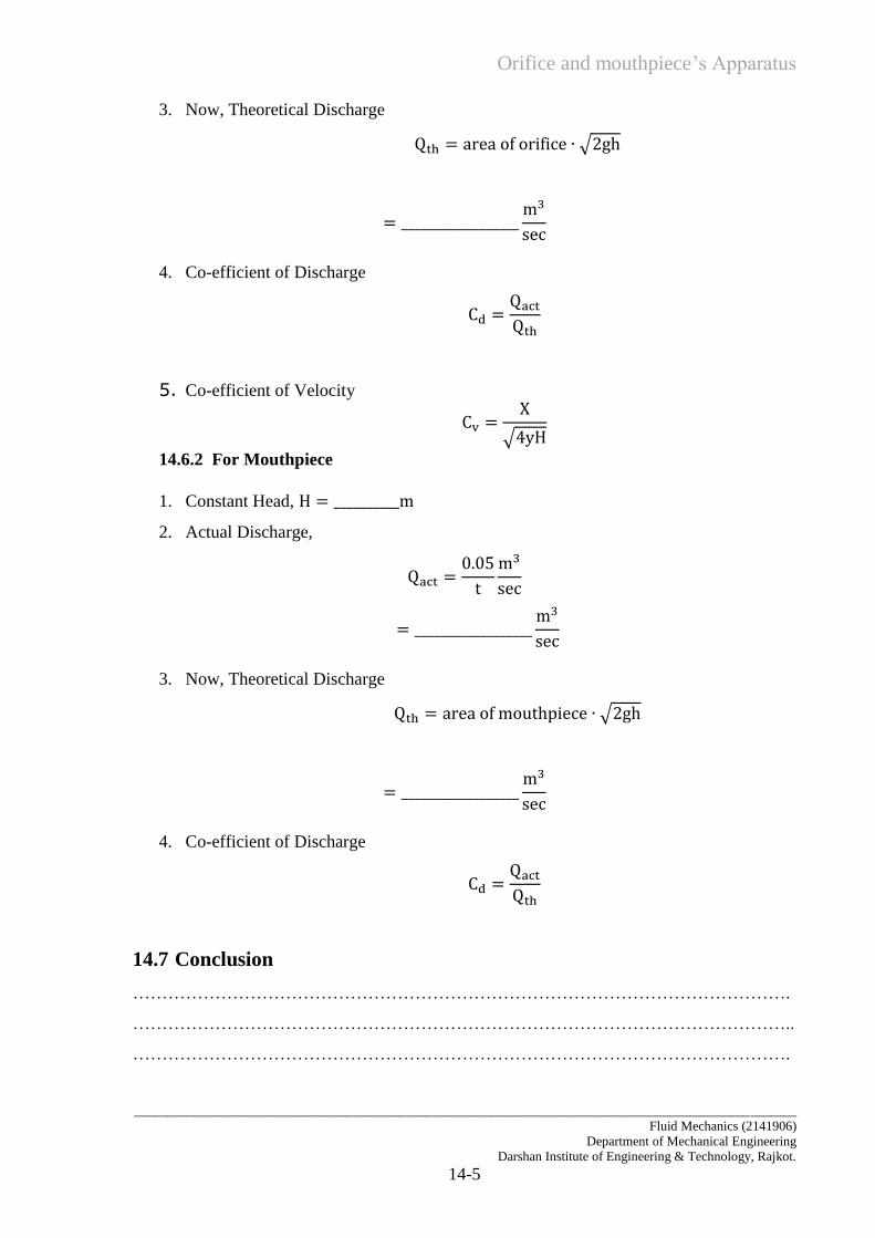
Orifice and mouthpiece’s Apparatus
____________________________________________________________________________________________________
Fluid Mechanics (2141906)
Department of Mechanical Engineering
Darshan Institute of Engineering & Technology, Rajkot.
14-5
3. Now, Theoretical Discharge
√
4. Co-efficient of Discharge
5. Co-efficient of Velocity
√
14.6.2 For Mouthpiece
1. Constant Head,
2. Actual Discharge,
3. Now, Theoretical Discharge
√
4. Co-efficient of Discharge
14.7 Conclusion
………………………………………………………………………………………………….
…………………………………………………………………………………………………..
………………………………………………………………………………………………….