DANMARKS NATIONALBANK WORKING PAPERS

2002 • 1

Heino Bohn Nielsen Institute of Economics

University of Copenhagen and

Dan Knudsen

Economics, Danmarks Nationalbank

Robust estimation of the expected inflation

March 2002

The Working Papers of Danmarks Nationalbank describe research and development, often still ongoing, as a contribution to the professional debate.

The viewpoints and conclusions stated are the responsibility of the individual contributors, and do not necessarily reflect the views of Danmarks Nationalbank.

As a general rule, Working Papers are not translated, but are available in the original language used by the contributor.

Danmarks Nationalbank's Working Papers are published in PDF format at www.nationalbanken.dk. A free electronic subscription is also available at this Web site.

The subscriber receives an e-mail notification whenever a new Working Paper is published.

Please direct any enquiries to Danmarks Nationalbank, Information Desk, Havnegade 5, DK-1093 Copenhagen K Denmark Tel.: +45 33 63 70 00 (direct) or +45 33 63 63 63 Fax : +45 33 63 71 03 E-mail:info@nationalbanken.dk

Nationalbankens Working Papers beskriver forsknings- og udviklingsarbejde, ofte af foreløbig karakter, med henblik på at bidrage til en faglig debat.

Synspunkter og konklusioner står for forfatternes regning og er derfor ikke nødvendigvis udtryk for Nationalbankens holdninger.

Working Papers vil som regel ikke blive oversat, men vil kun foreligge på det sprog, forfatterne har brugt.

Danmarks Nationalbanks Working Papers er tilgængelige på Internettet www.nationalbanken.dk i pdf-format. På webstedet er det muligt at oprette et gratis elektronisk abonnement, der leverer en e-mail notifikation ved enhver udgivelse af et Working Paper.

Henvendelser kan rettes til : Danmarks Nationalbank, Informationssektionen, Havnegade 5, 1093 København K. Telefon: 33 63 70 00 (direkte) eller 33 63 63 63 E-mail: info@nationalbanken.dk

Det er tilladt at kopiere fra Nationalbankens Working Papers - såvel elektronisk som i papirform - forudsat, at Danmarks Nationalbank udtrykkeligt anføres som kilde. Det er ikke tilladt at ændre eller forvanske indholdet.

ISSN (Print/tryk) 1602-1185

ISSN (online) 1602-1193

Robust estimation of the expected inßation

Heino Bohn NielsenInstitute of Economics,University of Copenhagen

Studiestræde 6DK-1455 Copenhagen K

heino.bohn.nielsen@econ.ku.dk

Dan KnudsenEconomics Department,Danmarks Nationalbank

Havnegade 5DK-1093 Copenhagen Kdkn@nationalbanken.dk

July 2, 2001

Abstract

Ignoring items with large price changes may enhance the informational content of aprice index. As an application of the metrically trimmed mean (Kim, 1992) we suggestto discard the individual price changes that deviate the most from the median. Focusingon outliers increases the efficiency compared to always trimming equally in both tailsand the implied bias problem seems small. The distribution of price changes is oftenskewed strongly to the right or to the left in a speciÞc month but is much closer tosymmetric for a longer period as a whole. This is also the case with Danish dataanalyzed in this paper. The suggested metrically trimmed mean gives a measure ofexpected inßation, which may help representing inßation in economic analyses.

Resume

Det kan forbedre informationen i et prisindeks at se bort fra poster med store prisæn-dringer. Som en anvendelse af det metriske trim (Kim,1992) foreslår vi at udelade deprisændringer, der afviger mest fra medianen. Et sådant fokus på de ekstreme værdierforbedrer efficiensen i forhold til altid at trimme i begge haler af fordelingen, og detmedfølgende bias-problem synes lille. Fordelingen af prisændringer er ofte stærkt højre-eller venstreskæv i en enkelt måned, men meget tættere på at være symmetrisk set overen længere periode. Det gælder også de danske data, der analyseres i nærværende pa-pir. Det foreslåede metriske trim giver et mål for forventet inßation, som kan være medtil at repræsentere inßationen i økonomiske analyser.

1

1 Introduction

Monthly inßation data typically show a considerable short-term variability, which reduces

their usefulness for economic analyses. The volatility distorts the autocorrelation of the

price series and the cross correlation to other economic time series. A simple reaction is to

use a moving average of monthly Þgures or a lower frequency. It is, however, not necessarily

all elements in the monthly price signal, which need to be downweighted. A big month-on-

month change in a price index is typically created by a few subindices changing a lot rather

than by all prices moving in parallel. Energy and unprocessed foods are typical candidates,

but sharp price changes are recorded for most products.

To address this problem, we view changes in the subindices as observations of stochastic

variables and proceed to estimate an expected increase in the consumer price index. If the

distribution of price changes were Gaussian the best estimate would be the actual increase

in the consumer price index. However, the outliers make the distribution of price changes

non-Gaussian and it improves the robustness of the estimation to reduce the weight of

extreme observations. A robust estimate of the price increase may serve as a measure of

the underlying inßation trend and it may be helpful for representing inßation or expected

inßation in economic analyses.

One frequently used robust estimator of the location of the central tendency of inßation

is the so-called trimmed mean, which discards the largest and smallest observations in a

given month and calculates the weighted mean of the remaining observations, see inter alia

Bryan, Cecchetti and Wiggins II (1997). The standard trimmed mean is a symmetric esti-

mator, which removes the same number of observations in both tails of the cross-sectional

distribution every month. Some authors have noted the scope for asymmetric estimators.

Roger (1997) reports that the distribution of individual inßation rates for New Zealand

is on average skewed to the right and he suggests trimming relative to the average mean

percentile to avoid a systematic difference between trimmed and actual inßation.

In this paper we are not particularly interested in the bias issue and suggest instead

to minimise the variance and to analyse what this stabilised measure of price increases

can be used for. Inspection of the data reveals that the skewness of price changes across

consumer goods varies between left and right. This shifting from month to month in the

position of outliers suggests that it may be efficient to allow trimming in only one tail

of the distribution instead of trimming both tails every month. SpeciÞcally, we propose

to apply the metrically trimmed mean from the median, see Kim (1992), and remove the

observations that deviate the most from the median. The paper further argues that it could

be preferable to remove whole subindices in the calculation rather than removing a precise

proportion of the weights. It is illustrated that the proposed estimator seems efficient under

a wide range of assumptions and the potential bias is small.

The rest of paper is organised as follows. Section 2 outlines the official Laspeyres

price index and characterises the distribution of prices changes, which looks highly non-

Gaussian. In section 3 some alternative robust measures of the inßation rate are discussed

and in section 4 they are evaluated. The chosen measure is presented in section 5 and some

applications are given. Finally, section 6 concludes.

2

2 The official index

The Danish consumer price index, Pt, is calculated as a Laspeyres index, i.e. as a weighted

arithmetic mean of 121 subindices

Pt =

P121i=1 PitQi0P121i=1 Pi0Qi0

=121Xi=1

αiPitPi0, (1)

where Pit and Qit are price and quantity of good i = 1, 2, ..., 121 at time t, and t = 0 is

the base period for the calculation. The weight αi = Pi0Qi0/P121j=1 Pj0Qj0 indicates the

share of good i in the budget of the average consumer andP121i=1 αi = 1. The weights

concern a certain year, but the base year and hence the weights have on average changed

every 5 years. The subindices and the most recent weights are listed in table 3 and the

modiÞcations of the raw data applied in the current analysis are mentioned in the appendix.

In this paper we analyse the developments in the Danish consumer prices for the period

1981 : 1 − 2000 : 11. The focus is on month-to-month changes, and the price indicesare seasonally adjusted using X-11 to avoid that the variance is dominated by seasonal

variations. It is appropriate to rank relative changes in logs, so the Laspeyres index (1)

is approximated by cumulating the weighted average of the monthly inßation rates, πit =

log (Pit/Pit−1), i = 1, ..., 121, i.e. cumulating

πt =121Xi=1

αiπit. (2)

Using this approximation, the overall price increase in a given month is the average of

individual price increases. To mimic a Laspeyres index the weights in (2) should in principle

be corrected every month to allow for relative price changes. However, the approximation

with Þxed weights is rather good as illustrated in Þgure 1 (A) and (B), which show the

change month-to-month and year-to-year respectively in the CPI seasonally adjusted and

in the approximation. In the rest of the paper, we use the approximation (2) as the baseline

inßation measure.

The big picture of the Danish inßation from the beginning of the eighties till 2000

reßects the impact of the hard currency policy adopted in 1982. One of the accompanying

measures was to abolish the price indexation of wages. The drop in inßation in the nineties

to around two per cent came while the economy was weak, but it conÞrms a fundamental

change over the sample that wage and price increases have responded only moderately to

the economic upturn in the last half of the nineties.

The distribution of price changes. It is apparent from Þgure 1 (A) that the monthly

inßation rate ßuctuates a lot, and a single observation seems to contain little information on

the tendency of the price development. To gain some insight on the variability we calculate

for each of the 238 months in the sample the weighted mean, πt, of the 121 price changes

{πit}121i=1, the weighted standard deviation, σt, and the weighted skewness and kurtosis. The

3

(A) (B)

Official consumer price index and approximationPrice change month on month (per cent)

1981 1984 1987 1990 1993 1996 1999-1.0

-0.5

0.0

0.5

1.0

1.5

2.0

2.5OfficialApproximation

Official consumer price index and approximationPrice change year on year (per cent)

1982 1985 1988 1991 1994 1997 20000

2

4

6

8

10

12OfficialApproximation

Figure 1. (A) and (B) compare the official consumer price index and the logarithmic approximation.

latter are the normalized third and fourth moment respectively, i.e.

mrt =121Xi=1

αi

µπit − πtσt

¶r, r = 3, 4,

which relate the empirical distribution to the Gaussian that has a skewness of zero and

a kurtosis of 3. Table 1 characterises the 238 distributions in the sample. The kurtosis

is usually far greater than 3 indicating that most distributions are leptokurtic, i.e. have

fat tails compared to the Gaussian distribution. The skewness exhibits large variation

from month to month in a range of −20 to 20, but on average the calculated skewness isclose to zero1. To illustrate we also calculate for each month the percentile of the ordered

observations equivalent to the weighted mean. This mean percentile ßuctuates in a wide

range of 0.14 to 0.88 but has mean and median just above and below 0.50. Bryan et al.

(1997) note that samples drawn from a symmetric but leptokurtic distribution are often

skewed.

There are several possible factors behind the outliers, which give the price distribution

its leptokurtic form. Price cartels may destabilise the price setting. Changing harvest

outcomes, new technology and new products, sales to reduce stocks, animal disease etc.,

all create price swings. A broad explanation of price jumps is found in the theory of menu

costs (Ball and Mankiw, 1995). If it is costly to change prices, they are presumably changed

less frequently but in larger steps. A practical point is that the recorded price change in a

subindex may be particularly large when the statistical agency substitutes a representative

good by a new. In general, it may increase the outliers if a subindex is only based on a

few representative goods. Moreover, the impact of indirect taxes and subsidies normally

comes stepwise and also politically administered prices may move abruptly for instance at

the start of a budget year.

1The measures used so far to characterize the distributions are themselves non-robust because the stan-

dardization is based on the sample mean and standard deviation. Several robust characterizations are

possible, but that is not the aim of this section.

4

Table 1: Characteristics of the distribution of price changes over the sample.

Statistic Mean Median St. dev. Minimum Maximum

Mean 0.303 0.242 0.333 -0.512 2.486Standard deviation 1.189 1.059 0.595 0.434 5.882Kurtosis 26.515 16.397 34.527 2.595 382.059Skewness 0.412 0.375 5.223 -22.122 17.723Mean percentile 0.507 0.494 0.170 0.136 0.884

Note: Mean, median, standard deviation, minimum and maximum over the sample of238 observations for some statistics of the cross sectional distributions {πit}121i=1.

3 Robust estimators

A simple way to deal with the noise in inßation data is to consider price developments

over several months, which downweights all information in the current inßation Þgures.

An alternative way to stabilise the inßation measure is to reduce the weight of the largest

of the 121 monthly price changes. This is the essence of robust estimation. We consider

the 121 monthly price changes as drawn from a distribution with all the non-Gaussian

characteristics described in the previous section. The arithmetic mean is the least squares

estimator, which is consistent and would be optimal if the distribution were Gaussian. The

fat tails and high probability of outliers, however, destroys the efficiency of the mean since

one extreme observation can remove the mean of the observations signiÞcantly from the

expected price increase. Robust estimators focus on the central part of the distribution,

which makes them less vulnerable.

A classical robust estimator is the median, which implies minimisation of absolute

deviations. The median is extremely robust but is potentially inefficient by only using

quantitative information from one observation. A class of estimators often used to calculate

robust inßation measures is the trimmed means, of which the median is a special case.

Instead of giving a weight of zero to all observations but the median one, the trimmed

mean assigns the weight zero to a smaller proportion of the subindices and calculates the

weighted mean of the remaining subindices.

Symmetrical trim. Usually in the case of price data the trimming is done symmetrically

by removing observations corresponding to a weight of 100 · µ/2 per cent from each tail

of the sample distribution each month. This is called the 100 · µ per cent symmetricallytrimmed mean and is calculated as

eπµt = 1

1− µ121Xi=1

αiπit1nFµ/2j [πjt] < πit < F

1−µ/2j [πjt]

o,

where e.g. Fµ/2j [·] is the µ/2−percentile (over j) of the cross section in square brackets and1 {·} is the indicator function. For µ = 0 the estimator eπµt is equal to the arithmetic meanand for µ → 1 the result converges to the median. This symmetrically trimmed mean is

applied to price data in several studies, inter alia Bryan et al. (1997), Mio and Higo (1999)

5

and Bryan and Cecchetti (1999b). Bakhshi and Yates (1999) discuss some drawbacks of

the approach.

Several authors have noted the possible advantage of asymmetric estimators. Roger

(1997) reports that the distribution of price changes for New Zealand on average is skewed

to the right and he suggests to trim relative to the average mean percentile, in the speciÞc

example to trim in both tails of the distribution relative to the 57th percentile, i.e. to

100 · µ/2 − 7 per cent in the right hand tail and 100 · µ/2 + 7 per cent in the left handtail in each month. This is done to avoid an indicator with a full sample mean below the

actual inßation, and the efforts entail a deliberate loss in efficiency. A mean at say the

57th percentile normally implies that most outliers appear in the right hand tail, but most

observations are trimmed in the left hand tail of the distribution.

Metrical trim. We prefer to put emphasis on variance reduction when trimming. The

preceding section illustrated that the dominant position of outliers changes between the

left and right tail. Thus, to focus on eliminating outliers one should not trim both tails

with preset percentages but trim the 100 · µ per cent of the observations that deviate themost from the median, i.e.

bπµt = 1

1− µ121Xi=1

αiπit1n¯̄πit − F 0.5j [πjt]

¯̄< F 1−µj

£πjt − F 0.5k [πkt]

¤o.

This is an application of the metrically trimmed mean from the median, see Kim (1992).

This trimming is ßexible in the sense that when the distribution is skewed to the right,

most observations are trimmed in the right hand tail and vice versa. Kim (1992) notes that

for symmetric distributions, the metrically trimmed mean is consistent and asymptotically

Gaussian. The breakdown point of the estimator is µ against µ/2 for the symmetrically

trimmed mean, which implies that a certain level of robustness can be achieved at the loss

of fewer observations and less information.

It may reduce the volatility further to remove whole subindices in the calculation of

the metrically trimmed mean instead of down-weighting the marginal index. Intuitively, it

seems strange to stop trimming in the middle of an index, and any non-negligible remain

of a marginal index may be more like an outlier than a part of the central distribution.

The counterpart to removing whole indices is that the de facto trimming percentage varies

over time and 100 · µ per cent is a minimum2.

4 Test of estimators

Three estimators are tested in this section: The metrical trim with removal of whole

subindices, the metrical trim with precise trim percentage and the symmetrical trim with

precise trim percentage. First, a Monte Carlo simulation is performed to illustrate the

relative virtues of the estimators. Second, bootstrap drawings from the price data are ap-2Removing whole indices is not relevant for symmetric trimming as it destroys the symmetry.

6

plied to conÞrm the Monte Carlo set-up and to determine the optimal estimator and trim

percentage for the present data set.

Monte Carlo simulation. The Monte Carlo set-up is designed to imitate some impor-

tant features of the empirical distribution of price changes. Most observations are drawn

from a standard Gaussian distribution, but 10 per cent of the observations are contam-

inated with noise, in the sense that they are drawn from a more dispersed or displaced

Gaussian distribution, i.e.

πit = (1− sit) · $it + sit · ft · ηit,

for i = 1, ..., 121, t = 1, ..., T , where

$it ∼ N (0, 1) and ηit ∼ N (a, b) .

Here sit is binomial distributed with probability P (sit = 1) = 0.1 for contamination, and ftis a binomial distributed sign shift with probability P (ft = 1) = d. The sign shift implies

that the noisy observations are drawn from either N (a, b) or N (−a, b), i.e. the locationof potential outliers changes between left and right and the distribution is on average

symmetric if a = 0 or γ = 0.5. In the simulation we consider the values a = 0, 3; b = 1, 3, 6,

d = 0.5, 0.6 and for each combination (a, b, d) we draw T = 1000 cross sections and trim

the data using the three methods and applying the most recent set of weights.

In the choice of estimator, πµt , there is a traditional trade-off between bias and efficiency.

We measure the bias as the average deviation from the expected value, i.e.

Bias (πµt ) =1

T

TXt=1

(πµt −E [πt]) ,

while the efficiency is measured as the variance of the trimmed series

V ar (πµt ) =1

T − 1TXt=1

Ãπµt −

1

T

TXi=1

πµi

!2.

A standard weighting of the bias an efficiency is the Mean Squared Error given byMSE =T−1T V ar (πµt ) + (Bias (π

µt ))

2.

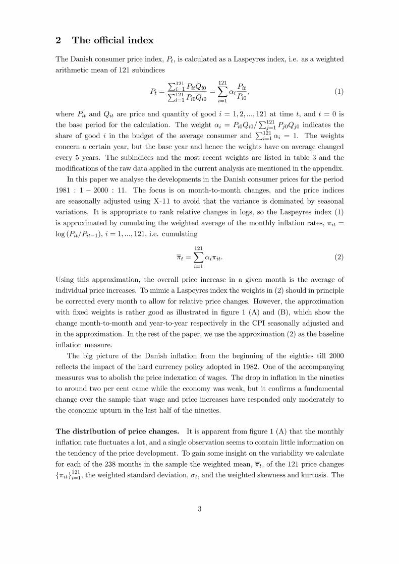
The results are reported in Þgure 2 for the bias, variance and MSE. In the Þrst column

(0, b, 0.5), the distribution is fully symmetric but is leptokurtic for b > 1. In the second

column (3, b, 0.5), the contamination is drawn from a displaced distribution and the skew-

ness change from month to month. On average, however, the distribution is symmetric

and E [πt] = 0. In the last column (3, b, 0.6), the combined distribution is skewed and on

average more outliers are located in the right hand tail.

For the standard Gaussian distribution, a = 0, b = 1, all estimators are consistent and

the bias is in all cases negligible. The simple arithmetic mean is as expected preferable

to the trimmed means in terms of variance. This result is mirrored in cases with minor

deviations from the Gaussian distribution. As either the dispersion or the numerical mean

7

of the contaminating distribution increases, implying fat tails and/or skewness in the sample

distributions, the scope for the trimmed means increases. If the distribution is on average

skewed, we observe a trade-off between bias and efficiency, but the bias problem looks small

compared to the variance reduction, and the MSE is in all cases practically indistinguisable

from the variance. The metrically trimmed mean is as expected marginally more biased

than the symmetrically but is strongly preferable in terms of efficiency.3

One important difference between the results for the metric and the symmetric esti-

mator is that the lowest variance of the metric estimator is typically obtained with a trim

percentage close to the contamination probability δ = 0.1. With the symmetric estima-

tor a much larger proportion of the observations have to be discarded to obtain efficient

estimates, and often the most efficient candidate is close to the median.

It also appears to marginally reduce the variance of the metrical trim to remove entire

subindices rather than to use a precise trim percentage. The difference is clearest in the

case of modest trim percentages.

Bootstrap. To analyse how the above Monte Carlo results translate to the data set,

we use a bootstrap strategy to approximate the underlying price distribution, see inter

alia Bryan and Cecchetti (1999b). We assume to have 121 distributions characterising the

subindices, and 238 observations on each distribution. We now construct t = 1, ..., 1000

bootstrap cross sections by drawing (with replacement) one observation from each distri-

bution i = 1, 2, ..., 121 in each month. In order to eliminate the effect of the change over

time in the overall inßation rate and to focus on the short-term variation, the trend in

all subindices has been removed with an HP Þlter4. The results regarding variance are

illustrated in Þrst part of table 25.

The outcome is similar to the Monte Carlo simulations with high kurtosis. More specif-

ically, cases (0, 6, 0.5), (3, 6, 0.5) and (3, 6, 0.6) in Þgure 2 resemble the empirical price

distribution. The overall lowest variance is obtained by trimming 25 per cent using the

metrically trimmed mean and removing whole indices. This estimator reduces the variance

by over 75 per cent, and is chosen as the preferred in the following.

The bootstrap results on relative variability are repeated when applying the three trim

methods to the historical data 1981−2000. Second part of table 2 illustrates the variance ofthe trimmed historical data calculated around the full sample means of the series. Again the

3The result on relative efficiency also holds for e.g. a uniform contaminating distribution instead of a

Gaussian, and the conclusions are robust to other measures of efficiency such as Mean Absolute Deviation.4A smoothing of λ = 1000 was chosen, but that is not crucial for the results. Using an HP trend to

represent the mean of the distribution obviously implies a measurement error. It is assumed that these

errors are too small to matter in a characterization of outliers and their impact.5The applied ordinary bootstrap algorithm eliminates the correlation structure of the data set. To assess

the robustness of the results to the autocorrelation of the price changes, the stationary bootstrap algorithm

of Politis and Romano (1994) was also applied. The idea is to draw several consecutive price changes

at a time, where the block length is geometrically distributed around a Þxed mean. This preserves the

autocorrelation within the drawn blocks. We also tried to draw contemporaneous blocks for all subindices,

thus preserving also the cross correlation between the subindices. The outcome was in all cases very similar

to the results reported for the ordinary bootstrap.

8

Bias

b=1

b=3

b=6

a=0,d=0.5 a=3,d=0.5 a=3,d=0.6

0 25 50 75 1000.0000

0.0045

0.0090

0.0135

0 25 50 75 100-0.0050

0.0000

0.0050

0.0100

0.0150

0 25 50 75 1000.000

0.005

0.010

0.015

0.020

0 25 50 75 100-0.006

0.000

0.006

0.012

0 25 50 75 100-0.0030

0.0000

0.0030

0.0060

0.0090

0.0120

0 25 50 75 100-0.0045

0.0000

0.0045

0.0090

0.0135

0 25 50 75 100-0.048

-0.032

-0.016

0.000

0.016

0 25 50 75 100-0.048

-0.036

-0.024

-0.012

-0.000

0.012

0 25 50 75 100-0.054

-0.036

-0.018

0.000

0.018

Variance

b=1

b=3

b=6

a=0,d=0.5 a=3,d=0.5 a=3,d=0.6

0 25 50 75 1001.0

1.5

2.0

2.5

0 25 50 75 1000.72

0.90

1.08

1.26

1.44

0 25 50 75 1000.25

0.50

0.75

1.00

0 25 50 75 1000.5

0.6

0.7

0.8

0.9

1.0

0 25 50 75 1000.25

0.50

0.75

1.00

0 25 50 75 1000.2

0.4

0.6

0.8

1.0

0 25 50 75 1000.5

0.6

0.7

0.8

0.9

1.0

0 25 50 75 1000.25

0.50

0.75

1.00

0 25 50 75 1000.2

0.4

0.6

0.8

1.0

MSE

b=1

b=3

b=6

a=0,d=0.5 a=3,d=0.5 a=3,d=0.6

0 25 50 75 1001.0

1.5

2.0

2.5

0 25 50 75 1000.72

0.90

1.08

1.26

1.44

0 25 50 75 1000.25

0.50

0.75

1.00

0 25 50 75 1000.5

0.6

0.7

0.8

0.9

1.0

0 25 50 75 1000.25

0.50

0.75

1.00

0 25 50 75 1000.2

0.4

0.6

0.8

1.0

0 25 50 75 1000.5

0.6

0.7

0.8

0.9

1.0

0 25 50 75 1000.25

0.50

0.75

1.00

0 25 50 75 1000.2

0.4

0.6

0.8

1.0

Metrically, whole indices

Metrically, precise

Symmetrically, precise

Figure 2: Monte Carlo Results. Bias, variance and MSE as a function of trim percentage.

9

Table 2: Variance of the trimmed series relative to the variance of arithmetic mean.

Trim percentage 0 5 10 15 20 25 30 40 50 60 70 80 90 100Bootstrapped cross sections

Metrically, whole indices 1.000 .352 .254 .227 .218 .212 .224 .236 .253 .266 .260 .249 .261 .263Metrically, precise 1.000 .398 .331 .282 .252 .242 .243 .257 .273 .291 .293 .281 .270 .263Symmetrically, precise 1.000 .549 .441 .400 .372 .347 .324 .275 .240 .227 .227 .238 .252 .263

Historical data

Metrically, whole indices 1.000 .456 .341 .277 .252 .239 .244 .260 .263 .273 .276 .278 .279 .276Metrically, precise 1.000 .515 .363 .311 .278 .253 .247 .256 .266 .272 .269 .271 .279 .276Symmetrically, precise 1.000 .738 .581 .488 .429 .392 .369 .333 .310 .300 .290 .280 .271 .276

Note.: The bootstrap is based on 1000 simulations and the most recent set of weigths.

most stable estimate with a variance around 14 of that in the untrimmed mean is obtained

with the metrically trimmed mean and a trim percentage of 25. For the symmetrically

trimmed mean, the most stable estimate is close to the median.

The true expected inßation is a theoretical magnitude, and we can only address the bias

issue by making some assumptions. If for instance we want the same mean as the actual

inßation over the full sample 1981−2000, we should add 0.37 per cent p.a. to the trimmedinßation rate. Taking this as a bias measure implies that the squared bias amounts to 1 per

cent of the difference in variance between trimmed and actual inßation. That is a relative

magnitude as in the Monte Carlo experiment where for (0, 6, 0.6) the squared bias amounts

to 12 per cent of the variance reduction at a trim percentage of 25. Instead of adding 0.37

per cent p.a. the sample mean of the actual inßation could also be reproduced by a metrical

trim from the 60 percentile, but this would increase the simple variance in the measure by

approximately 25 per cent compared to the preferred metrical trim from the median.

5 Results and applications

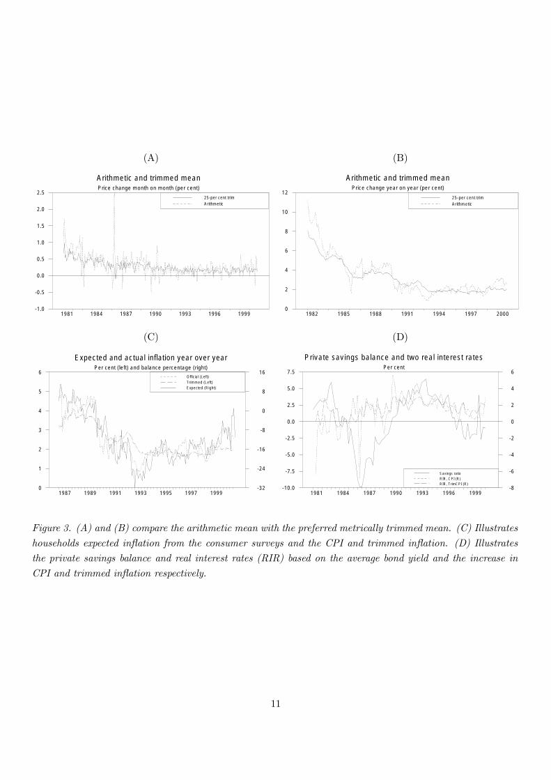
The changes in the arithmetic mean and in the preferred 25−per cent metrically trimmedmean from month to month and from year to year respectively are illustrated in Þgure

3 (A) and (B). The trimmed mean suggests a more stable picture where the underlying

inßation is unchanged over most of the nineties. It appears that the sample difference

in the year-on-year increases mostly relates to the Þrst years where the overall inßation

was still high. Thereafter the difference between trimmed and untrimmed mean becomes

more unsystematic. The mentioned difference to actual inßation of 0.37 per cent p.a. for

1981− 2000 is reduced to a very insigniÞcant 0.14 per cent p.a. for 1983− 2000.Due to the strategy of excluding whole subindices, the de facto trim percentage changes

over time. For the chosen sample and 25 per cent nominal trim the actual trimming

percentage varies between precisely 25.00 and 42.71 per cent with an average of 26.56 per

cent. The high trimming percentage that particular month reßects that subindex 54 of

housing is the marginal index in the calculation.

Table 3 given on the last page illustrates how often the different subindices are removed

in the preferred 25 per cent trimmed mean. As expected the prices of fuels and gasoline and

of some unprocessed food articles disappear relatively often. A good part of the sales effect

on garments is removed by the seasonal Þlter, but the timing of the winter and summer

sales varies and leaves a lot of irregular price movements in not least women�s garments.10

(A) (B)

Arithmetic and trimmed meanPrice change month on month (per cent)

1981 1984 1987 1990 1993 1996 1999-1.0

-0.5

0.0

0.5

1.0

1.5

2.0

2.525-per cent trimArithmetic

Arithmetic and trimmed meanPrice change year on year (per cent)

1982 1985 1988 1991 1994 1997 20000

2

4

6

8

10

1225-per cent trimArithmetic

(C) (D)

Expected and actual inflation year over yearPer cent (left) and balance percentage (right)

1987 1989 1991 1993 1995 1997 19990

1

2

3

4

5

6

-32

-24

-16

-8

0

8

16Official (Left)Trimmed (Left)Expected (Right)

Private savings balance and two real interest ratesPer cent

1981 1984 1987 1990 1993 1996 1999-10.0

-7.5

-5.0

-2.5

0.0

2.5

5.0

7.5

-8

-6

-4

-2

0

2

4

6

Savings ratioRIR, CPI (R)RIR, TrimCPI (R)

Figure 3. (A) and (B) compare the arithmetic mean with the preferred metrically trimmed mean. (C) Illustrates

households expected inßation from the consumer surveys and the CPI and trimmed inßation. (D) Illustrates

the private savings balance and real interest rates (RIR) based on the average bond yield and the increase in

CPI and trimmed inßation respectively.

11

Prediction of inßation. The volatility of monthly CPI movements disturbs the auto-

correlation of monthly price increases, and it is better to predict the monthly change in

the full consumer price index by the less volatile monthly change in the trimmed index. A

simple estimation yields

log³

PtPt−1

´= 0.00830

(0.1)log³Pt−1Pt−2

´+ 1.08165

(7.5)log³ bPt−1bPt−2

´+ 0.00003

(0.0)

for t = 1981 : 3− 2000 : 11, where Pt is the price index accumulated from the arithmetic

mean, πt, and bPt is the index based on the 25 per cent metrically trimmed mean, bπ.25t .Figures in parentheses are t−values.

Removing the Þrst insigniÞcant term increases the coefficient for the change in the

trimmed index slightly to 1.092. A coefficient above one and a small positive constant lifts

the forecast mean a little to make it equal the untrimmed inßation mean in the estimation

sample. This automatic mean correction is not signiÞcant. Restricting the coefficient to

one and the constant to zero can be done with an insigniÞcant F (2, 235) statistic of 1.52.

Instead of the monthly price increase one often focuses on the relatively less volatile

year-on-year change in the price index. Two consecutive year-on-year index changes have

11 monthly changes in common, and the ability of bπ.25t to predict πt one month ahead can

be brought to use by replacing the actual monthly price change 12 months back by the

latest trimmed monthly change

log³

PtPt−12

´= − 0.0036

(0.1)log³Pt−1Pt−13

´+ 1.0110

(16.3)

³log³Pt−1Pt−12

´+ log

³ bPt−1bPt−2´´

− 0.0001(0.2)

The predictive gain reßects that a large price increase 11 months ago can make the present

year-on-year increase both large and likely to moderate in the following month. The ability

of the trimmed price change to predict the next actual price increase conÞrms that the

trimmed change indicates a central tendency. This may be one point of departure for

forecasting, but it goes without saying that other information can make the forecasted

price increase differ from the latest observation on the trimmed increase.

Besides, the large price changes trimmed away are sometimes relevant to the forecasting.

A jump in energy prices may Þrst leave the trimmed inßation unchanged, but if energy prices

stay up and trigger second round effects it will turn into a general price increase.

Household price expectations. The price expectations of Danish households have been

measured by the monthly consumer survey since 1987. The answers to the survey�s standard

question on price increases are transformed to an index, which should correlate positively

with the price increase expected over the coming 12 months. It turns out that this survey

index correlates nicely with the year-on-year increase in the actual price index, better than

with the year-on-year increase in the trimmed price index, cf. Þgure 3 (C).

Thus, households seem to expect the present headline inßation to repeat itself in the next

12 months. SpeciÞcally, households do not seem to weigh down the largest price movements.

This may reßect that households get their information from the press mentioning the present

headline inßation. Moreover, the press and the public debate are likely to focus on large

12

movements in say energy, meat or coffee prices. However, the trimmed price increase may

still be the most relevant for the investment and consumption decisions of economic agents.

Real interest rate. Another test could be to compare the use of trimmed inßation

versus actual inßation in explaining consumption and investment. This amounts to testing

whether trimmed price increases works better in the real rate of interest.

To simplify we concentrate on the private savings balance, i.e. savings minus invest-

ments in the total private sector comprising households and companies. This macro ap-

proach is facilitated by the Danish currency peg, which implies that the interest rate is

given from abroad and not determined by the savings balance. The national account Þg-

ures applied are quarterly and the price increases used are also quarterly. The nominal

interest rate is the average bond yield after tax.

None of the two real interest rates (RIR) correlate that well with the savings balance,

cf. Þgure 3 (D). SpeciÞcally, it seems difficult to explain the private savings balance during

the eighties using only real interest rates. However, the real interest based on the trimmed

price increase is less erratic and seems to be doing a little better as also indicated by a

simple estimation

Savings balance = 2.16784(4.0)

Interest rate − 0.17588(0.7)

log³

PtPt−1

´− 1.20755

(2.3)log³ bPtbPt−1

´− 0.05552

(3.2)

estimated for quarterly data for t = 1981 : 2− 2000 : 3.

6 Conclusion

This paper has focused on the trimmed mean as a robust estimator of expected inßation.

The pattern of price changes over the last 20 years led us to prefer a metrical trim, which

removes the largest outliers regardless of their sign. This seems to be the most efficient

trim also taking into account the enhanced risk of bias compared to a symmetric trim. A

bootstrap simulation suggested a trim percentage of 25 for the proposed metrical trim, and

it indicated a minor advantage in removing whole subindices at a time instead of sticking

to the 25 per cent sharp.

The trimmed inßation rate suggests a more stable picture of the actual inßation. This

stabilised measure may be used to represent inßation or expected inßation in economic

analyses, e.g. in applications involving a real interest rate. Trimmed inßation responds

when the price development is general rather than concentrated on a few products. Fur-

thermore the noise reduction enhances the correlation structure, which improves the ability

of the trimmed rate to predict inßation. We are not suggesting to make this the only input

in an inßation forecast, but the trimmed inßation could be a starting point.

In the economic policy framework, it may be advantageous to include a focus on the

inßation trend represented by the trimmed inßation rate.

13

Appendix: The data

The price data used are the 121 subindices in the Danish CPI for the period January 1981

till November 2000, cf. table 3. All price data including the weighting scheme are from

Statistics Denmark.

Statistics Denmark�s revisions of weights are included in the calculation of our log

indicator for the CPI. In the sample period the weight basis for the CPI was revised in

April 1984, January 1991, September 1996 and December 1999. For instance the 121

monthly price changes March 1984 to April 1984 are weighted by the Þrst set of weights,

price changes April 1984 to May 1984 by the second. These revisions are intended to keep

the content of the CPI up to date.

For one small item, services not included elsewhere, we did not have the official index

but applied the price index for the main category miscellaneous goods up to 1991. Similarly,

the price of the transport category is used for a small transport item, which only appears

1991-1996. These deviations to the official CPI calculation are too small to affect the

results. Another minor data issue is that all subindices in the past were published without

decimals although decimals were used for the calculation of the CPI. The increases the

data noise but there is no remedy and, anyway, our log approximation based on a weighted

average of changes in subindices comes close to the published CPI.

Consumers� price expectations are taken from Statistics Denmark�s monthly consumer

surveys. The quarterly private savings balance and the bond yield are from the data bank

of the Mona model, Danmarks Nationalbank.

14

References

[1] Bakhshi, H. and T. Yates (1999) To trim or not to trim ? An application of the

trimmed mean inßation estimator to the United Kingdom, Bank of England, Working

Paper No. 97.

[2] Ball, L. and N.G. Mankiw (1995) Relative price changes as aggregate supply shocks,

The Quarterly Journal of Economics, 110, 1, 161-193.

[3] Bryan, M.F. and S.G. Cecchetti (1999a) Inßation and the distribution of price changes,

Review of Economics and Statistics, 81, 188-196.

[4] ��� and ��� (1999b) The Monthly Measurement of Core Inßation in Japan,

Bank of Japan, Institute for Monetary and Economic Studies, Discussion Paper No.

99-E-4.

[5] ���, ���and R.L. Wiggins II (1997) Efficient Inßation Estimation, NBERWork-

ing Paper No. 6183.

[6] Cecchetti, S.G. (1997) Measuring Short-run Inßation for Central Bankers, Economic

Review of the Federal Reserve Bank of St. Louis, 79, 143-156.

[7] Kim, S.-J. (1992) The Metrically Trimmed Mean as a Robust Estimator of Location,

The Annals of Statistics, 20, 3, 1534-1547.

[8] Mio, H. and M. Higo (1999) Underlying Inßation and the Distribution of Price Changes

- Evidence from the Japanese Trimmed Mean CPI, Bank of Japan, Institute for Mon-

etary and Economic Studies, Discussion Paper No. 99-E-5.

[9] Politis, D.N. and J.P. Romano (1994) The Stationary Bootstrap, Journal of the Amer-

ican Statistical Association, 89, 428, 1303-1313.

[10] Roger, S. (1997) A robust Measure of Inßation in New Zealand 1949-96, Reserve Bank

of New Zealand, Discussion Paper No. G97/7.

15

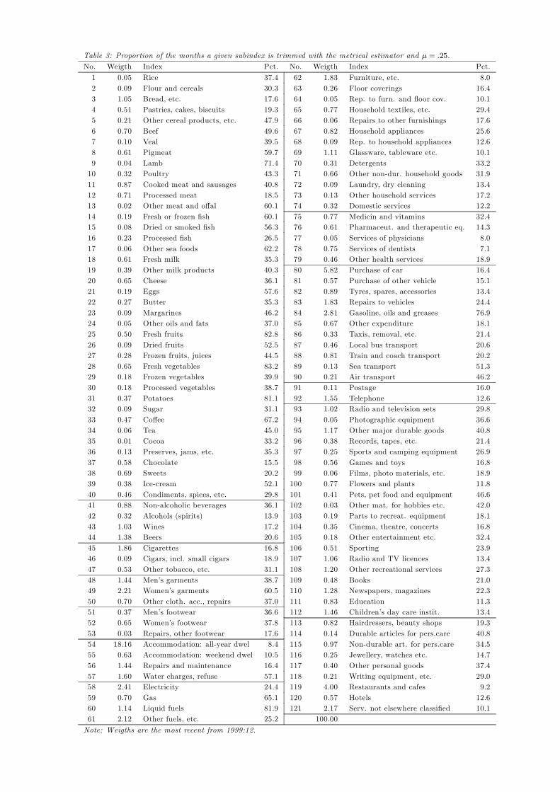
Table 3: Proportion of the months a given subindex is trimmed with the metrical estimator and µ = .25.

No. Weigth Index Pct. No. Weigth Index Pct.

1 0.05 Rice 37.4 62 1.83 Furniture, etc. 8.02 0.09 Flour and cereals 30.3 63 0.26 Floor coverings 16.43 1.05 Bread, etc. 17.6 64 0.05 Rep. to furn. and ßoor cov. 10.14 0.51 Pastries, cakes, biscuits 19.3 65 0.77 Household textiles, etc. 29.45 0.21 Other cereal products, etc. 47.9 66 0.06 Repairs to other furnishings 17.66 0.70 Beef 49.6 67 0.82 Household appliances 25.67 0.10 Veal 39.5 68 0.09 Rep. to household appliances 12.68 0.61 Pigmeat 59.7 69 1.11 Glassware, tableware etc. 10.19 0.04 Lamb 71.4 70 0.31 Detergents 33.210 0.32 Poultry 43.3 71 0.66 Other non-dur. household goods 31.911 0.87 Cooked meat and sausages 40.8 72 0.09 Laundry, dry cleaning 13.412 0.71 Processed meat 18.5 73 0.13 Other household services 17.213 0.02 Other meat and offal 60.1 74 0.32 Domestic services 12.214 0.19 Fresh or frozen Þsh 60.1 75 0.77 Medicin and vitamins 32.415 0.08 Dried or smoked Þsh 56.3 76 0.61 Pharmaceut. and therapeutic eq. 14.316 0.23 Processed Þsh 26.5 77 0.05 Services of physicians 8.017 0.06 Other sea foods 62.2 78 0.75 Services of dentists 7.118 0.61 Fresh milk 35.3 79 0.46 Other health services 18.919 0.39 Other milk products 40.3 80 5.82 Purchase of car 16.420 0.65 Cheese 36.1 81 0.57 Purchase of other vehicle 15.121 0.19 Eggs 57.6 82 0.89 Tyres, spares, accessories 13.422 0.27 Butter 35.3 83 1.83 Repairs to vehicles 24.423 0.09 Margarines 46.2 84 2.81 Gasoline, oils and greases 76.924 0.05 Other oils and fats 37.0 85 0.67 Other expenditure 18.125 0.50 Fresh fruits 82.8 86 0.33 Taxis, removal, etc. 21.426 0.09 Dried fruits 52.5 87 0.46 Local bus transport 20.627 0.28 Frozen fruits, juices 44.5 88 0.81 Train and coach transport 20.228 0.65 Fresh vegetables 83.2 89 0.13 Sea transport 51.329 0.18 Frozen vegetables 39.9 90 0.21 Air transport 46.230 0.18 Processed vegetables 38.7 91 0.11 Postage 16.031 0.37 Potatoes 81.1 92 1.55 Telephone 12.632 0.09 Sugar 31.1 93 1.02 Radio and television sets 29.833 0.47 Coffee 67.2 94 0.05 Photographic equipment 36.634 0.06 Tea 45.0 95 1.17 Other major durable goods 40.835 0.01 Cocoa 33.2 96 0.38 Records, tapes, etc. 21.436 0.13 Preserves, jams, etc. 35.3 97 0.25 Sports and camping equipment 26.937 0.58 Chocolate 15.5 98 0.56 Games and toys 16.838 0.69 Sweets 20.2 99 0.06 Films, photo materials, etc. 18.939 0.38 Ice-cream 52.1 100 0.77 Flowers and plants 11.840 0.46 Condiments, spices, etc. 29.8 101 0.41 Pets, pet food and equipment 46.641 0.88 Non-alcoholic beverages 36.1 102 0.03 Other mat. for hobbies etc. 42.042 0.32 Alcohols (spirits) 13.9 103 0.19 Parts to recreat. equipment 18.143 1.03 Wines 17.2 104 0.35 Cinema, theatre, concerts 16.844 1.38 Beers 20.6 105 0.18 Other entertainment etc. 32.445 1.86 Cigarettes 16.8 106 0.51 Sporting 23.946 0.09 Cigars, incl. small cigars 18.9 107 1.06 Radio and TV licences 13.447 0.53 Other tobacco, etc. 31.1 108 1.20 Other recreational services 27.348 1.44 Men�s garments 38.7 109 0.48 Books 21.049 2.21 Women�s garments 60.5 110 1.28 Newspapers, magazines 22.350 0.70 Other cloth. acc., repairs 37.0 111 0.83 Education 11.351 0.37 Men�s footwear 36.6 112 1.46 Children�s day care instit. 13.452 0.65 Women�s footwear 37.8 113 0.82 Hairdressers, beauty shops 19.353 0.03 Repairs, other footwear 17.6 114 0.14 Durable articles for pers.care 40.854 18.16 Accommodation: all-year dwel 8.4 115 0.97 Non-durable art. for pers.care 34.555 0.63 Accommodation: weekend dwel 10.5 116 0.25 Jewellery, watches etc. 14.756 1.44 Repairs and maintenance 16.4 117 0.40 Other personal goods 37.457 1.60 Water charges, refuse 57.1 118 0.21 Writing equipment, etc. 29.058 2.41 Electricity 24.4 119 4.00 Restaurants and cafes 9.259 0.70 Gas 65.1 120 0.57 Hotels 12.660 1.14 Liquid fuels 81.9 121 2.17 Serv. not elsewhere classiÞed 10.161 2.12 Other fuels, etc. 25.2 100.00

Note: Weigths are the most recent from 1999:12.