1

Bernoulli equation

Daniel Bernoulli (1710-1782)

2

Bernoulli: preamble

Want to discuss the properties of a moving fluid.

Will do this initially under the simplest possible

conditions, leading to Bernoulli’s equation. The

following restrictions apply.

• Flow is inviscid, there are no viscous drag forces

• Heat conduction is not possible for an inviscid

flow

• The fluid is incompressible .

• The flow is steady (velocity pattern constant).

• The paths traveled by small sections of the fluid

are well defined.

• Will be implicitly using the Euler equations of

motion (discussed later)

3

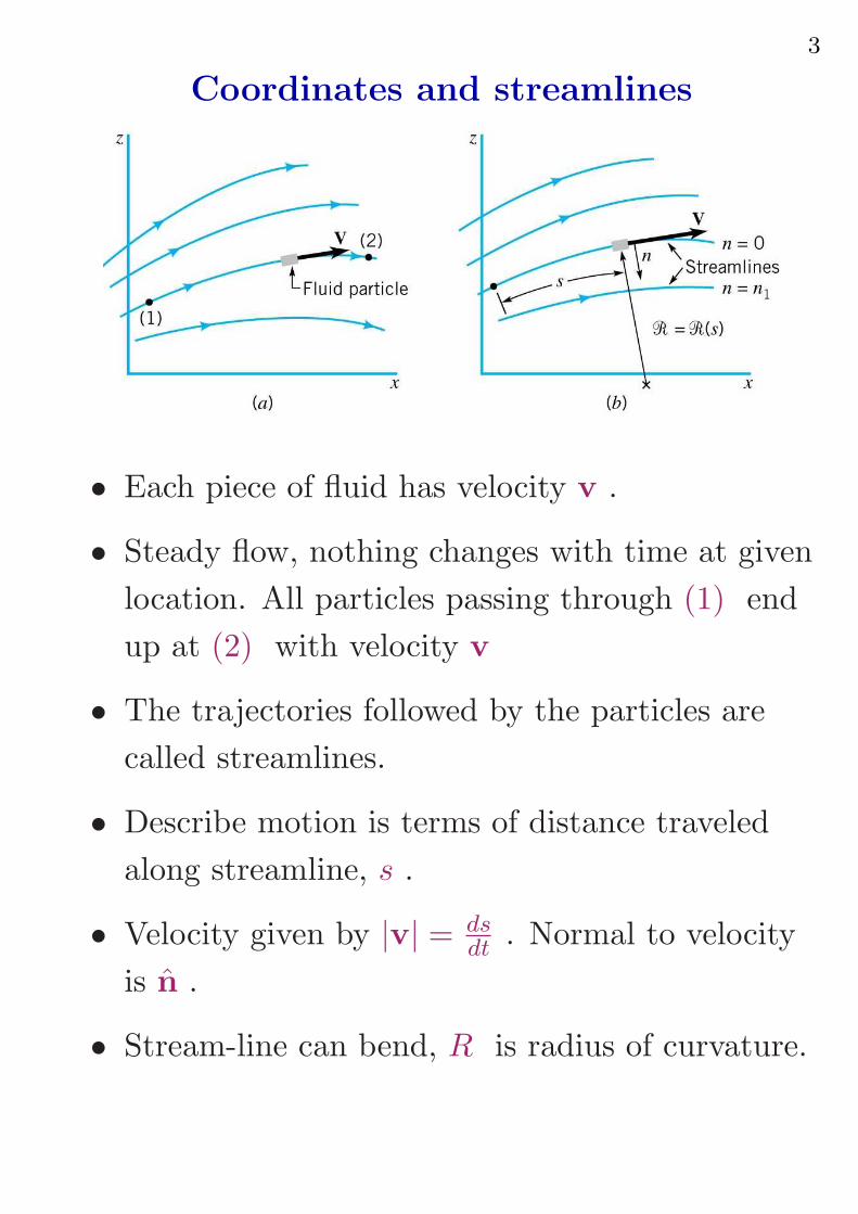
Coordinates and streamlines

• Each piece of fluid has velocity v .

• Steady flow, nothing changes with time at given

location. All particles passing through (1) end

up at (2) with velocity v

• The trajectories followed by the particles are

called streamlines.

• Describe motion is terms of distance traveled

along streamline, s .

• Velocity given by |v| = dsdt

. Normal to velocity

is n .

• Stream-line can bend, R is radius of curvature.

4

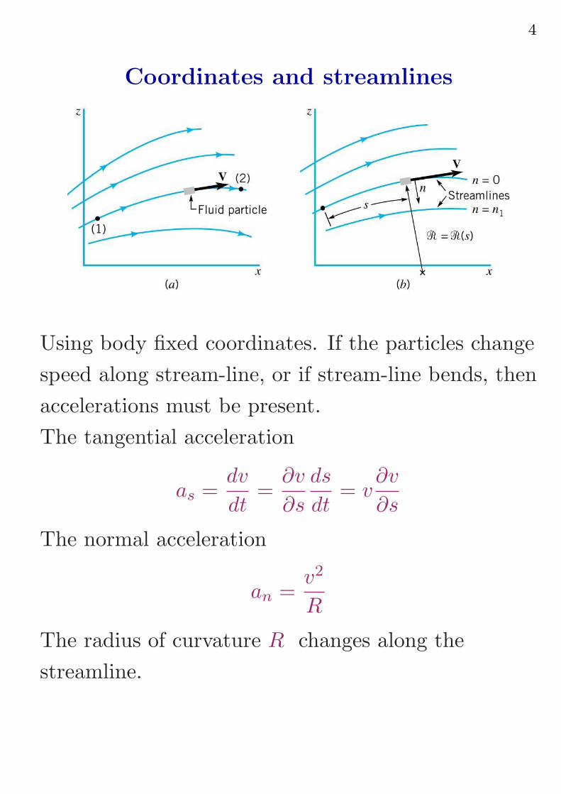
Coordinates and streamlines

Using body fixed coordinates. If the particles change

speed along stream-line, or if stream-line bends, then

accelerations must be present.

The tangential acceleration

as =dv

dt=

∂v

∂s

ds

dt= v

∂v

∂s

The normal acceleration

an =v2

R

The radius of curvature R changes along the

streamline.

5

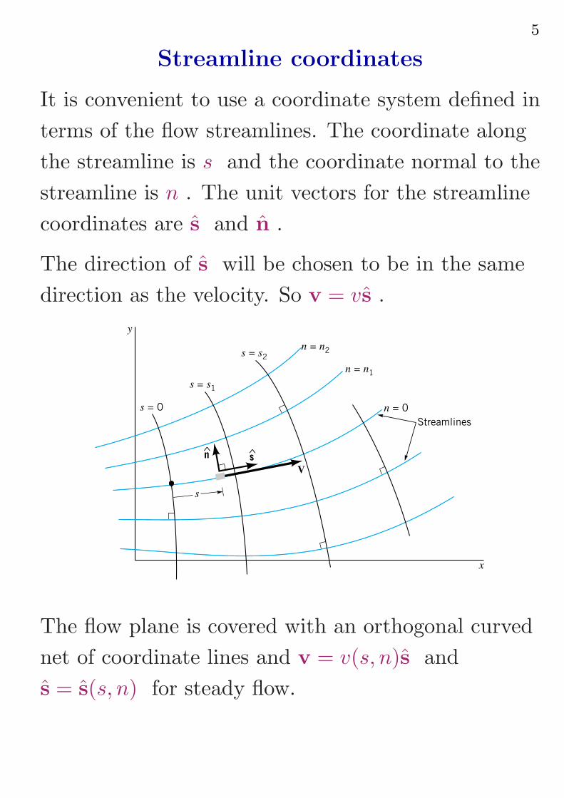
Streamline coordinates

It is convenient to use a coordinate system defined in

terms of the flow streamlines. The coordinate along

the streamline is s and the coordinate normal to the

streamline is n . The unit vectors for the streamline

coordinates are s and n .

The direction of s will be chosen to be in the same

direction as the velocity. So v = vs .

s

n^

s^

V

s = 0

s = s1

s = s2

n = n2

n = n1

n = 0

Streamlines

y

x

The flow plane is covered with an orthogonal curved

net of coordinate lines and v = v(s, n)s and

s = s(s, n) for steady flow.

6

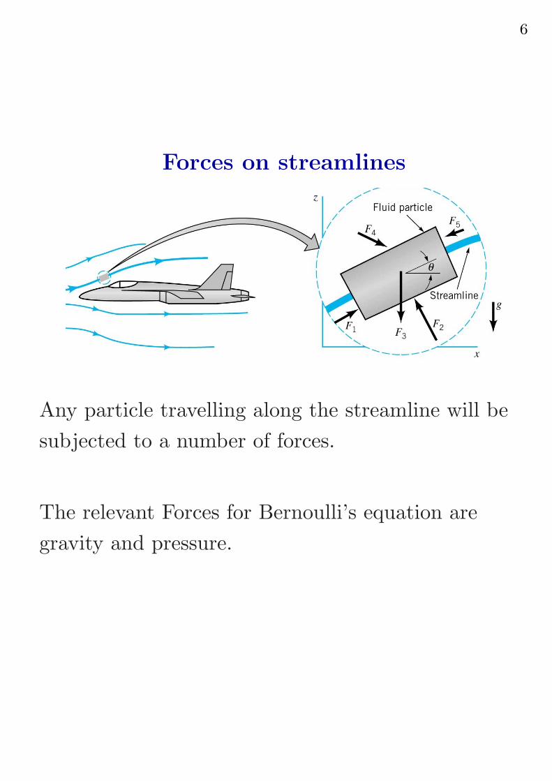
Forces on streamlines

Any particle travelling along the streamline will be

subjected to a number of forces.

The relevant Forces for Bernoulli’s equation are

gravity and pressure.

7

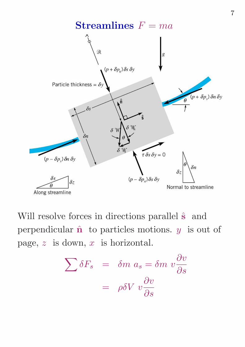
Streamlines F = ma

Will resolve forces in directions parallel s and

perpendicular n to particles motions. y is out of

page, z is down, x is horizontal.

∑

δFs = δm as = δm v∂v

∂s

= ρδV v∂v

∂s

8

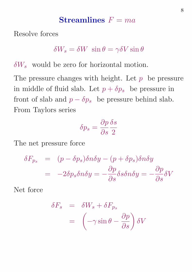
Streamlines F = ma

Resolve forces

δWs = δW sin θ = γδV sin θ

δWs would be zero for horizontal motion.

The pressure changes with height. Let p be pressure

in middle of fluid slab. Let p + δps be pressure in

front of slab and p − δps be pressure behind slab.

From Taylors series

δps =∂p

∂s

δs

2

The net pressure force

δFps= (p − δps)δnδy − (p + δps)δnδy

= −2δpsδnδy = −∂p

∂sδsδnδy = −∂p

∂sδV

Net force

δFs = δWs + δFps

=

(

−γ sin θ − ∂p

∂s

)

δV

9

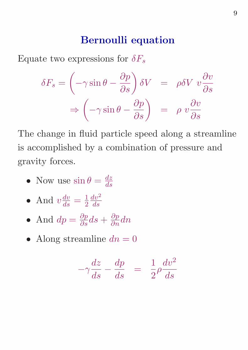
Bernoulli equation

Equate two expressions for δFs

δFs =

(

−γ sin θ − ∂p

∂s

)

δV = ρδV v∂v

∂s

⇒(

−γ sin θ − ∂p

∂s

)

= ρ v∂v

∂s

The change in fluid particle speed along a streamline

is accomplished by a combination of pressure and

gravity forces.

• Now use sin θ = dzds

• And v dvds

= 1

2

dv2

ds

• And dp = ∂p∂s

ds + ∂p∂n

dn

• Along streamline dn = 0

−γdz

ds− dp

ds=

1

2ρdv2

ds

10

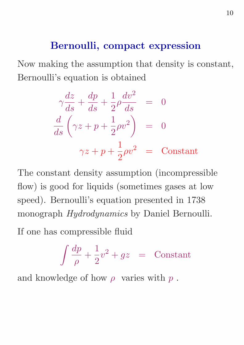
Bernoulli, compact expression

Now making the assumption that density is constant,

Bernoulli’s equation is obtained

γdz

ds+

dp

ds+

1

2ρdv2

ds= 0

d

ds

(

γz + p +1

2ρv2

)

= 0

γz + p +1

2ρv2 = Constant

The constant density assumption (incompressible

flow) is good for liquids (sometimes gases at low

speed). Bernoulli’s equation presented in 1738

monograph Hydrodynamics by Daniel Bernoulli.

If one has compressible fluid∫

dp

ρ+

1

2v2 + gz = Constant

and knowledge of how ρ varies with p .

11

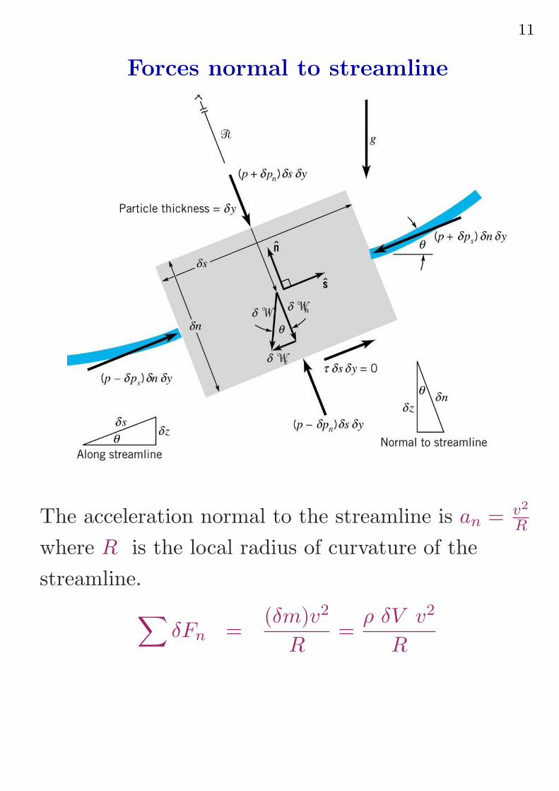
Forces normal to streamline

The acceleration normal to the streamline is an = v2

R

where R is the local radius of curvature of the

streamline.

∑

δFn =(δm)v2

R=

ρ δV v2

R

12

Forces normal to streamline

A change in stream direction occurs from pressure

and/or and gravity forces. Resolve forces

δWn = δW cos θ = γδV cos θ

δWn would be zero for vertical motion.

The pressure changes with height. Let p be pressure

in middle of fluid slab, p + δpn is pressure at top of

slab and p − δpn be pressure at bottom of slab.

From Taylors series

δpn =∂p

∂n

δn

2

The net pressure force, δFpn

δFpn= (p − δpn)δs δy − (p + δpn)δs δy

= −2δpnδn δy = −∂p

∂nδn δs δy = −∂p

∂nδV

Need to combine pressure and weight forces to get

net Force

13

Forces normal to streamline

Combine weight and pressure forces

δFn = δWn + δFpn

=

(

−γ cos θ − ∂p

∂n

)

δV =ρδV v2

R

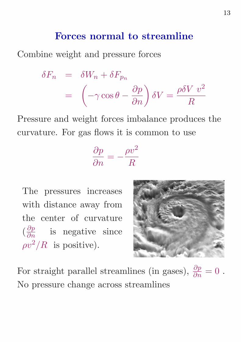
Pressure and weight forces imbalance produces the

curvature. For gas flows it is common to use

∂p

∂n= −ρv2

R

The pressures increases

with distance away from

the center of curvature

( ∂p∂n

is negative since

ρv2/R is positive).

For straight parallel streamlines (in gases), ∂p∂n

= 0 .

No pressure change across streamlines

14

Forces normal to streamline

Will consider fluid parameters normal to stream line(

γ cos θ +∂p

∂n

)

+ρv2

R= 0

• ∂p∂n

= dpdn

since s is constant.

• cos θ = dzdn

and so for incompressible flows

dp

dn+ γ

dz

dn+

ρv2

R= 0

dp

dn+ γ

dz

dn+

ρv2

R= 0

d

dn(p + γz) +

ρv2

R= 0

p + γz + ρ

∫

v2

Rdn = Constant

For a compressible substance, the best reduction is∫

dp

ρ+

∫

v2

R+ gz = Constant

15

Interpretation for incompressible flows

Along the streamline

γz + p +1

2ρv2 = Constant

Across the streamline

p + γz + ρ

∫

v2

Rdn = Constant

The units of Bernoulli’s equations are J m−3 . This

is not surprising since both equations arose from an

integration of the equation of motion for the force

along the s and n directions.

The Bernoulli equation along the stream-line is a

statement of the work energy theorem. As the

particle moves, the pressure and gravitational forces

can do work, resulting in a change in the kinetic

energy.

16

Dynamic and static pressures

p +1

2ρv2 + ρgz = constant

Static pressure is the pressure as measured moving

with the fluid. (e.g. static with fluid). This is the p

term in Bernoulli’s equation. Imagine moving along

the fluid with a pressure gauge.

Some times the ρgz term in Bernoulli’s equation is

called the hydrostatic pressure. (e.g. it is the change

in pressure due to change in elevation.)

Dynamic pressure is a pressure that occurs when

kinetic energy of the flowing fluid is converted into

pressure rise. This is the pressure associated with

the 1

2ρv2 term in Bernoulli’s equation.

17

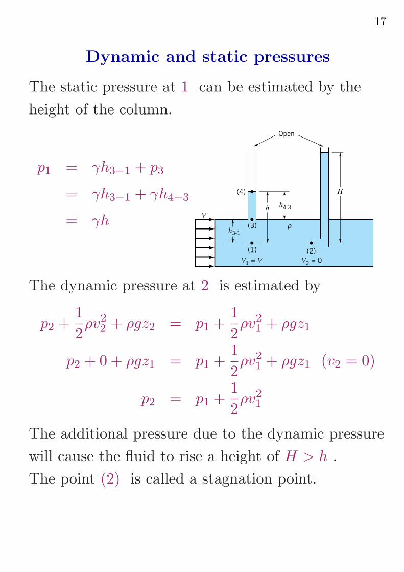
Dynamic and static pressures

The static pressure at 1 can be estimated by the

height of the column.

p1 = γh3−1 + p3

= γh3−1 + γh4−3

= γh

(1) (2)

(3)

(4)

h3-1

hh4-3

ρ

Open

H

V

V1 = V V2 = 0

The dynamic pressure at 2 is estimated by

p2 +1

2ρv2

2 + ρgz2 = p1 +1

2ρv2

1 + ρgz1

p2 + 0 + ρgz1 = p1 +1

2ρv2

1 + ρgz1 (v2 = 0)

p2 = p1 +1

2ρv2

1

The additional pressure due to the dynamic pressure

will cause the fluid to rise a height of H > h .

The point (2) is called a stagnation point.

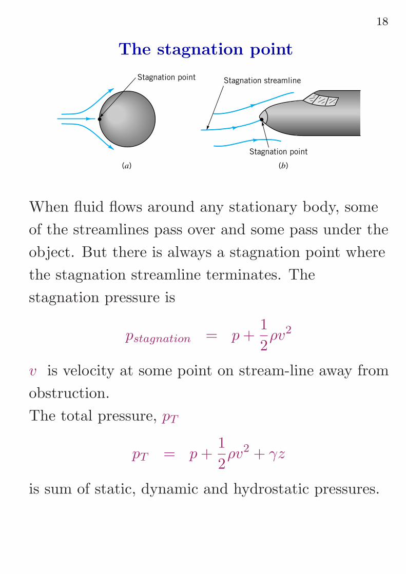
18

The stagnation point

Stagnation point

(a)

Stagnation streamline

Stagnation point

(b)

When fluid flows around any stationary body, some

of the streamlines pass over and some pass under the

object. But there is always a stagnation point where

the stagnation streamline terminates. The

stagnation pressure is

pstagnation = p +1

2ρv2

v is velocity at some point on stream-line away from

obstruction.

The total pressure, pT

pT = p +1

2ρv2 + γz

is sum of static, dynamic and hydrostatic pressures.

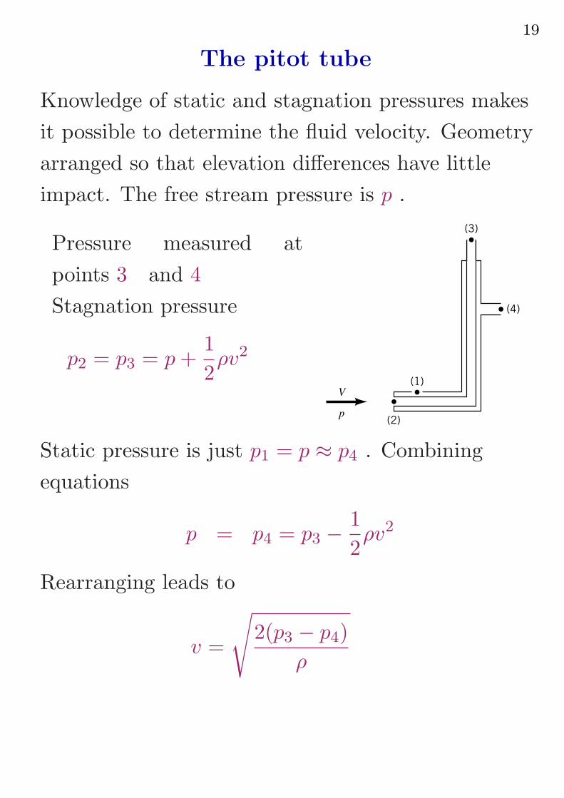
19

The pitot tube

Knowledge of static and stagnation pressures makes

it possible to determine the fluid velocity. Geometry

arranged so that elevation differences have little

impact. The free stream pressure is p .

Pressure measured at

points 3 and 4

Stagnation pressure

p2 = p3 = p +1

2ρv2

V

p

(1)

(2)

(4)

(3)

Static pressure is just p1 = p ≈ p4 . Combining

equations

p = p4 = p3 −1

2ρv2

Rearranging leads to

v =

√

2(p3 − p4)

ρ

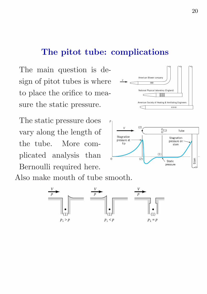
20

The pitot tube: complications

The main question is de-

sign of pitot tubes is where

to place the orifice to mea-

sure the static pressure.

V

American Blower company

National Physical laboratory (England)

American Society of Heating & Ventilating Engineers

The static pressure does

vary along the length of

the tube. More com-

plicated analysis than

Bernoulli required here.

Also make mouth of tube smooth.

21

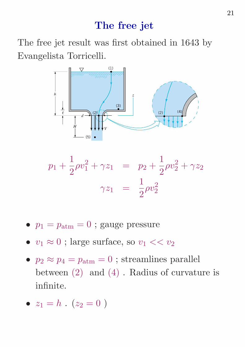
The free jet

The free jet result was first obtained in 1643 by

Evangelista Torricelli.

p1 +1

2ρv2

1 + γz1 = p2 +1

2ρv2

2 + γz2

γz1 =1

2ρv2

2

• p1 = patm = 0 ; gauge pressure

• v1 ≈ 0 ; large surface, so v1 << v2

• p2 ≈ p4 = patm = 0 ; streamlines parallel

between (2) and (4) . Radius of curvature is

infinite.

• z1 = h . (z2 = 0 )

22

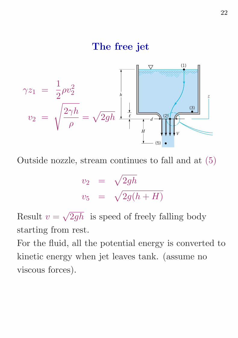
The free jet

γz1 =1

2ρv2

2

v2 =

√

2γh

ρ=

√

2gh

Outside nozzle, stream continues to fall and at (5)

v2 =√

2gh

v5 =√

2g(h + H)

Result v =√

2gh is speed of freely falling body

starting from rest.

For the fluid, all the potential energy is converted to

kinetic energy when jet leaves tank. (assume no

viscous forces).

23

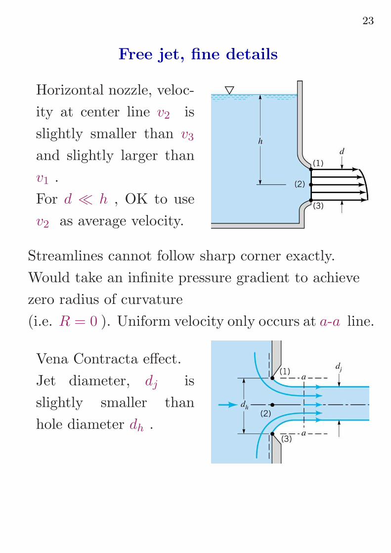
Free jet, fine details

Horizontal nozzle, veloc-

ity at center line v2 is

slightly smaller than v3

and slightly larger than

v1 .

For d ≪ h , OK to use

v2 as average velocity.

Streamlines cannot follow sharp corner exactly.

Would take an infinite pressure gradient to achieve

zero radius of curvature

(i.e. R = 0 ). Uniform velocity only occurs at a-a line.

Vena Contracta effect.

Jet diameter, dj is

slightly smaller than

hole diameter dh .

24

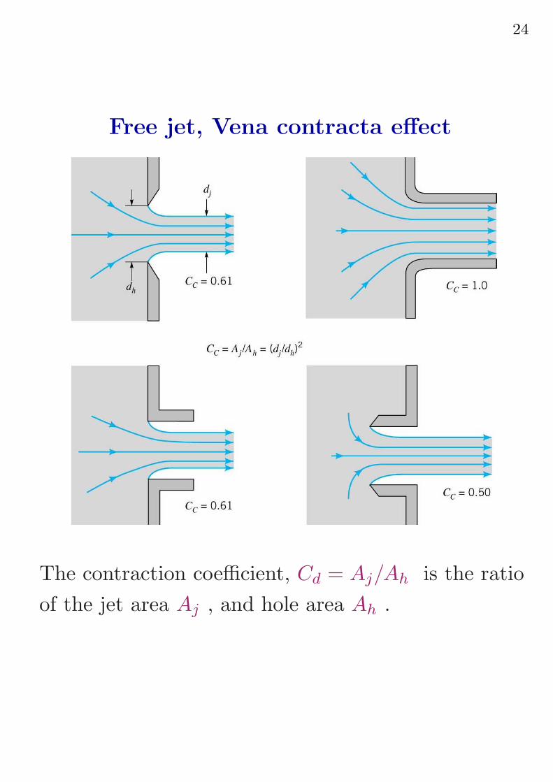
Free jet, Vena contracta effect

The contraction coefficient, Cd = Aj/Ah is the ratio

of the jet area Aj , and hole area Ah .

25

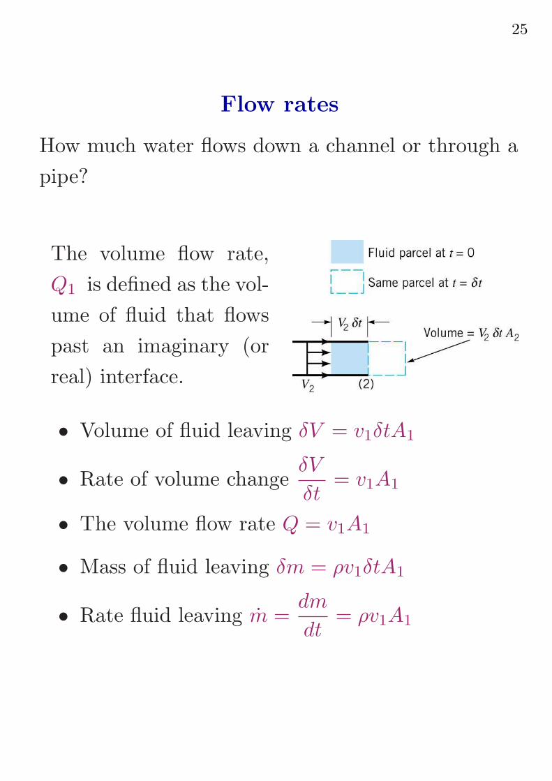
Flow rates

How much water flows down a channel or through a

pipe?

The volume flow rate,

Q1 is defined as the vol-

ume of fluid that flows

past an imaginary (or

real) interface.

• Volume of fluid leaving δV = v1δtA1

• Rate of volume changeδV

δt= v1A1

• The volume flow rate Q = v1A1

• Mass of fluid leaving δm = ρv1δtA1

• Rate fluid leaving m =dm

dt= ρv1A1

26

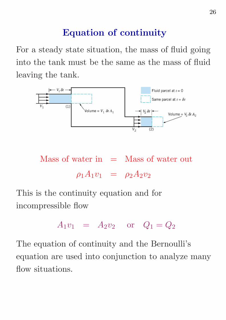
Equation of continuity

For a steady state situation, the mass of fluid going

into the tank must be the same as the mass of fluid

leaving the tank.

Mass of water in = Mass of water out

ρ1A1v1 = ρ2A2v2

This is the continuity equation and for

incompressible flow

A1v1 = A2v2 or Q1 = Q2

The equation of continuity and the Bernoulli’s

equation are used into conjunction to analyze many

flow situations.

27

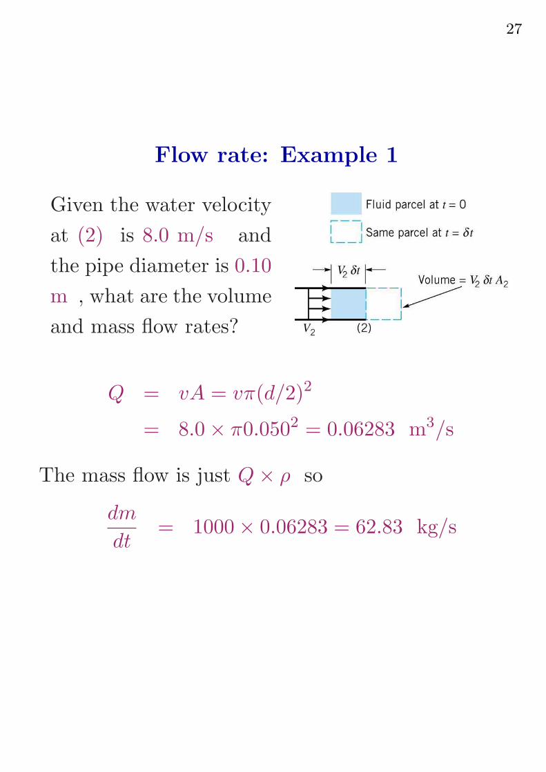
Flow rate: Example 1

Given the water velocity

at (2) is 8.0 m/s and

the pipe diameter is 0.10

m , what are the volume

and mass flow rates?

Q = vA = vπ(d/2)2

= 8.0 × π0.0502 = 0.06283 m3/s

The mass flow is just Q × ρ so

dm

dt= 1000 × 0.06283 = 62.83 kg/s

28

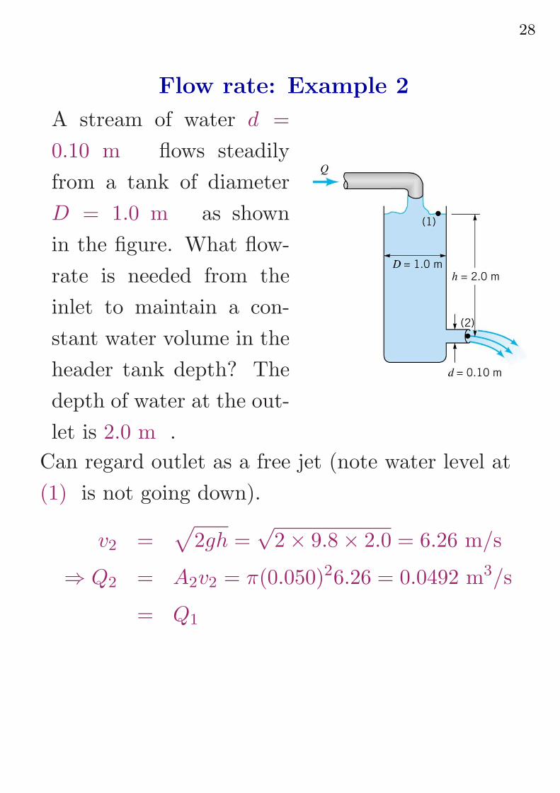
Flow rate: Example 2

A stream of water d =

0.10 m flows steadily

from a tank of diameter

D = 1.0 m as shown

in the figure. What flow-

rate is needed from the

inlet to maintain a con-

stant water volume in the

header tank depth? The

depth of water at the out-

let is 2.0 m .

Can regard outlet as a free jet (note water level at

(1) is not going down).

v2 =√

2gh =√

2 × 9.8 × 2.0 = 6.26 m/s

⇒ Q2 = A2v2 = π(0.050)26.26 = 0.0492 m3/s

= Q1

29

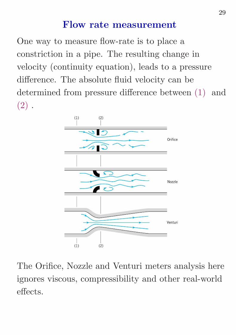
Flow rate measurement

One way to measure flow-rate is to place a

constriction in a pipe. The resulting change in

velocity (continuity equation), leads to a pressure

difference. The absolute fluid velocity can be

determined from pressure difference between (1) and

(2) .

The Orifice, Nozzle and Venturi meters analysis here

ignores viscous, compressibility and other real-world

effects.

30

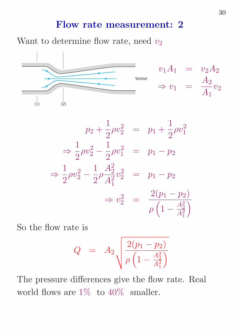
Flow rate measurement: 2

Want to determine flow rate, need v2

v1A1 = v2A2

⇒ v1 =A2

A1

v2

p2 +1

2ρv2

2 = p1 +1

2ρv2

1

⇒ 1

2ρv2

2 − 1

2ρv2

1 = p1 − p2

⇒ 1

2ρv2

2 − 1

2ρA2

2

A21

v2

2 = p1 − p2

⇒ v2

2 =2(p1 − p2)

ρ(

1 − A2

2

A2

1

)

So the flow rate is

Q = A2

√

√

√

√

2(p1 − p2)

ρ(

1 − A2

2

A2

1

)

The pressure differences give the flow rate. Real

world flows are 1% to 40% smaller.

31

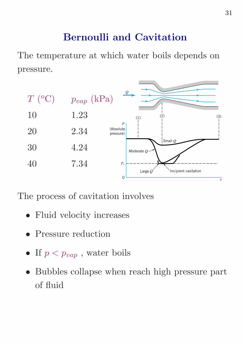
Bernoulli and Cavitation

The temperature at which water boils depends on

pressure.

T (oC) pvap (kPa)

10 1.23

20 2.34

30 4.24

40 7.34

Q

p

(Absolute

pressure)

(1)(2) (3)

Small Q

Moderate Q

Large Q Incipient cavitation

pv

0 x

The process of cavitation involves

• Fluid velocity increases

• Pressure reduction

• If p < pvap , water boils

• Bubbles collapse when reach high pressure part

of fluid

32

Bernoulli and Cavitation

Pressure transients exceeding 100 MPa can be

produced. These transients can produce structural

damage to surfaces.

33

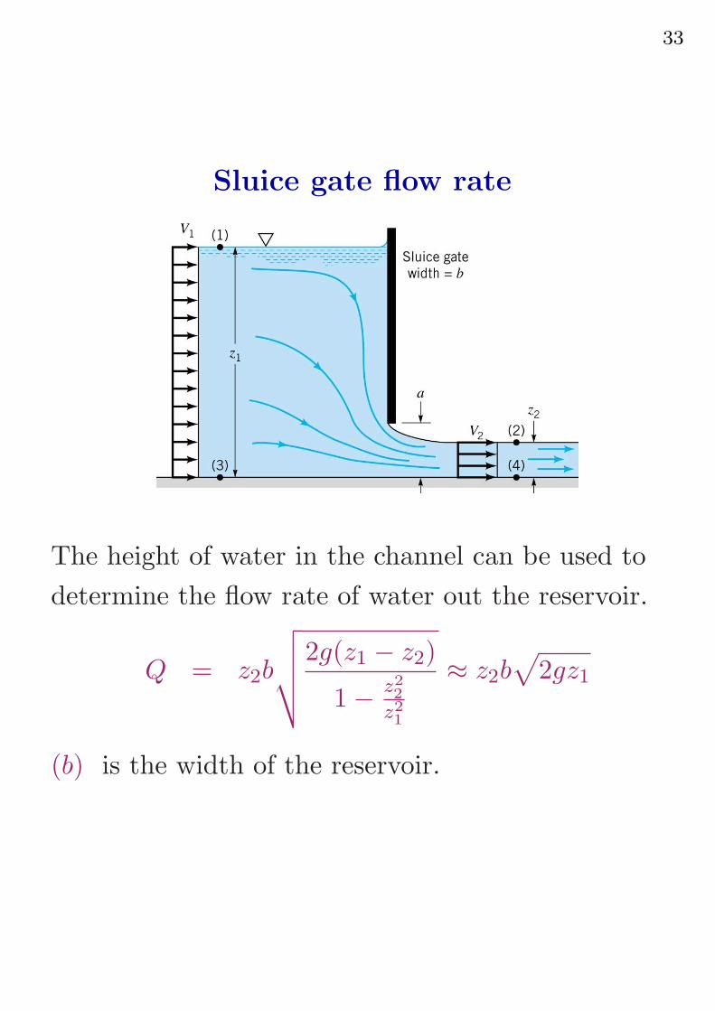
Sluice gate flow rate

The height of water in the channel can be used to

determine the flow rate of water out the reservoir.

Q = z2b

√

√

√

√

2g(z1 − z2)

1 − z2

2

z2

1

≈ z2b√

2gz1

(b) is the width of the reservoir.

34

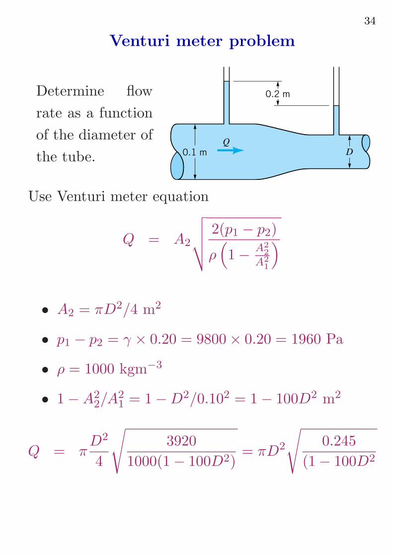
Venturi meter problem

Determine flow

rate as a function

of the diameter of

the tube.

0.2 m

Q

0.1 m D

Use Venturi meter equation

Q = A2

√

√

√

√

2(p1 − p2)

ρ(

1 − A2

2

A2

1

)

• A2 = πD2/4 m2

• p1 − p2 = γ × 0.20 = 9800 × 0.20 = 1960 Pa

• ρ = 1000 kgm−3

• 1 − A22/A2

1= 1 − D2/0.102 = 1 − 100D2 m2

Q = πD2

4

√

3920

1000(1 − 100D2)= πD2

√

0.245

(1 − 100D2

35

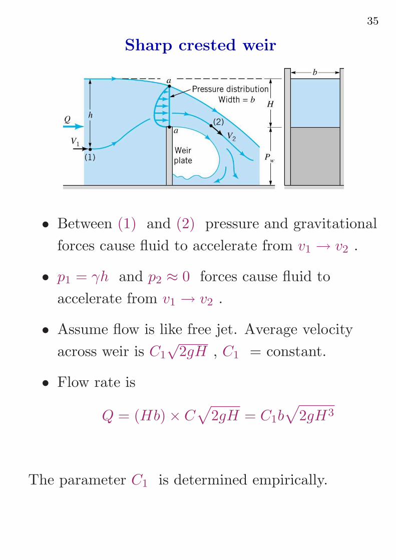
Sharp crested weir

• Between (1) and (2) pressure and gravitational

forces cause fluid to accelerate from v1 → v2 .

• p1 = γh and p2 ≈ 0 forces cause fluid to

accelerate from v1 → v2 .

• Assume flow is like free jet. Average velocity

across weir is C1

√2gH , C1 = constant.

• Flow rate is

Q = (Hb) × C√

2gH = C1b√

2gH3

The parameter C1 is determined empirically.

36

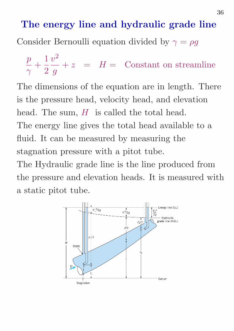
The energy line and hydraulic grade line

Consider Bernoulli equation divided by γ = ρg

p

γ+

1

2

v2

g+ z = H = Constant on streamline

The dimensions of the equation are in length. There

is the pressure head, velocity head, and elevation

head. The sum, H is called the total head.

The energy line gives the total head available to a

fluid. It can be measured by measuring the

stagnation pressure with a pitot tube.

The Hydraulic grade line is the line produced from

the pressure and elevation heads. It is measured with

a static pitot tube.

37

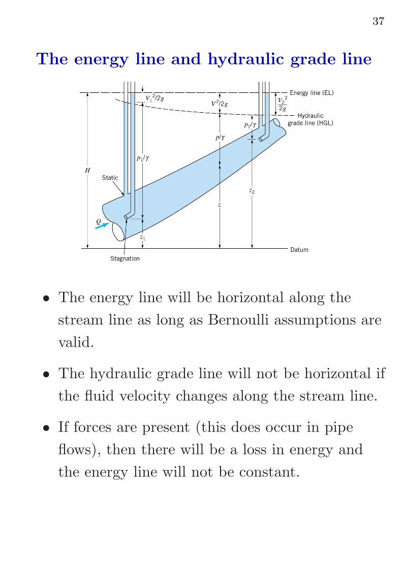
The energy line and hydraulic grade line

• The energy line will be horizontal along the

stream line as long as Bernoulli assumptions are

valid.

• The hydraulic grade line will not be horizontal if

the fluid velocity changes along the stream line.

• If forces are present (this does occur in pipe

flows), then there will be a loss in energy and

the energy line will not be constant.

38

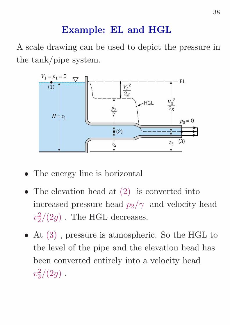
Example: EL and HGL

A scale drawing can be used to depict the pressure in

the tank/pipe system.

• The energy line is horizontal

• The elevation head at (2) is converted into

increased pressure head p2/γ and velocity head

v22/(2g) . The HGL decreases.

• At (3) , pressure is atmospheric. So the HGL to

the level of the pipe and the elevation head has

been converted entirely into a velocity head

v23/(2g) .

39

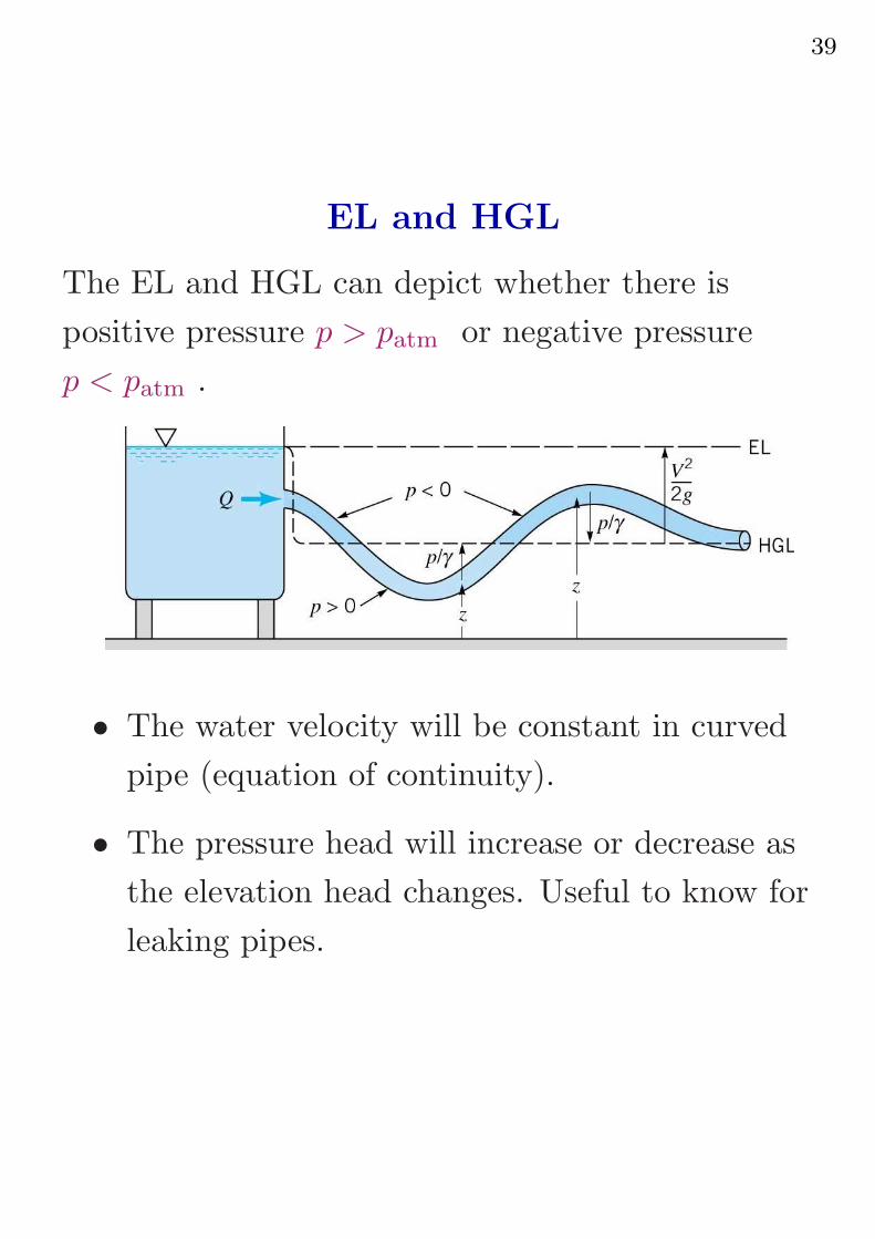
EL and HGL

The EL and HGL can depict whether there is

positive pressure p > patm or negative pressure

p < patm .

• The water velocity will be constant in curved

pipe (equation of continuity).

• The pressure head will increase or decrease as

the elevation head changes. Useful to know for

leaking pipes.

40

Limitations on Bernoulli equation

A number of problems can invalidate the use of the

Bernoulli equation, these are compressibility effects,

rotational effects, unsteady effects.

Compressibility effects

When can compressibility effects impact on gas

flows? Consider stagnation point

• Stagnation pressure is greater than static

pressure by 1

2ρv2 (dynamic pressure), provided

ρ constant.

• ρ will not changes too much as long as dynamic

pressure is not too large when compared to

static pressure.

• So flows at low v will be incompressible

• But dynamic pressure increases as v2 , so

compressibility effects most likely at high speed.

41

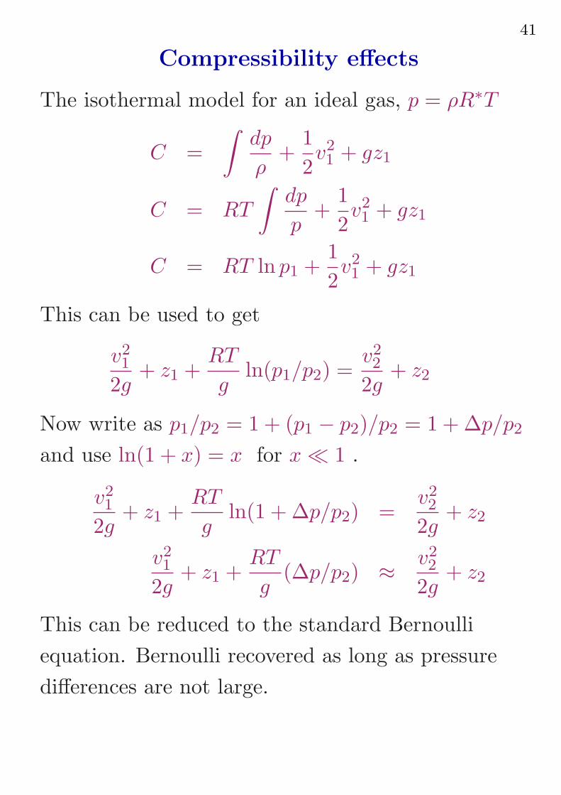
Compressibility effects

The isothermal model for an ideal gas, p = ρR∗T

C =

∫

dp

ρ+

1

2v2

1 + gz1

C = RT

∫

dp

p+

1

2v2

1 + gz1

C = RT ln p1 +1

2v2

1 + gz1

This can be used to get

v21

2g+ z1 +

RT

gln(p1/p2) =

v22

2g+ z2

Now write as p1/p2 = 1 + (p1 − p2)/p2 = 1 + ∆p/p2

and use ln(1 + x) = x for x ≪ 1 .

v21

2g+ z1 +

RT

gln(1 + ∆p/p2) =

v22

2g+ z2

v21

2g+ z1 +

RT

g(∆p/p2) ≈ v2

2

2g+ z2

This can be reduced to the standard Bernoulli

equation. Bernoulli recovered as long as pressure

differences are not large.

42

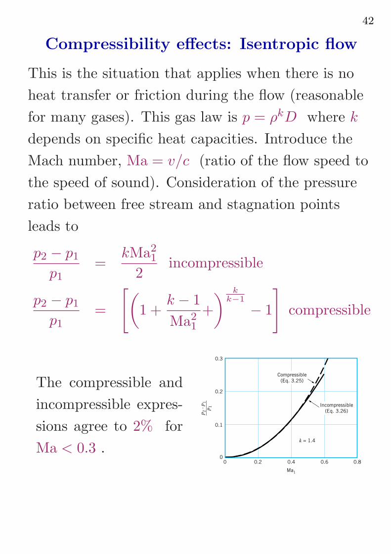
Compressibility effects: Isentropic flow

This is the situation that applies when there is no

heat transfer or friction during the flow (reasonable

for many gases). This gas law is p = ρkD where k

depends on specific heat capacities. Introduce the

Mach number, Ma = v/c (ratio of the flow speed to

the speed of sound). Consideration of the pressure

ratio between free stream and stagnation points

leads to

p2 − p1

p1

=kMa2

1

2incompressible

p2 − p1

p1

=

[

(

1 +k − 1

Ma2

1

+

)k

k−1

− 1

]

compressible

The compressible and

incompressible expres-

sions agree to 2% for

Ma < 0.3 .

Compressible

(Eq. 3.25)

Incompressible

(Eq. 3.26)

k = 1.4

0.3

0.2

0.1

00 0.2 0.4 0.6 0.8

Ma1

p2

– p

1______

p1

43

Unsteady effects

Implicit in the discussion was an assumption that

the fluid flows along steady state streamlines, so

v = v(s) is a function of position along the stream

and does not contain any explicit time dependence.

If v = v(s, t) then then it would be necessary to

include this when integrating along the streamline.

p1 +1

2ρv2

1 + γz1 = p2 +1

2ρv2

2 + γz2 + ρ

∫ t2

t1

∂p

∂sds

The additional term does complicate matters and

can only be easily handled under restricted

circumstances. There are quasi-steady flows where

some time dependence exists, but Bernoulli’s

equations could be applied as if the flow were steady

(e.g. the draining of a tank).

44

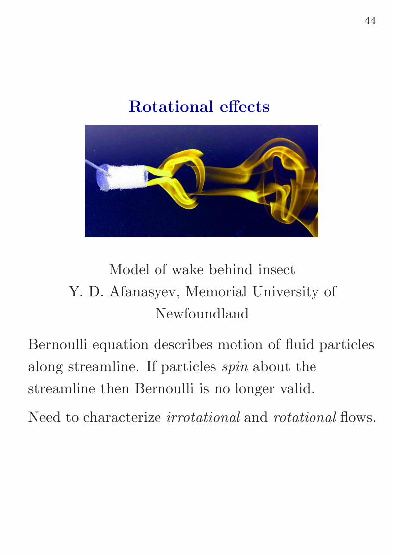
Rotational effects

Model of wake behind insect

Y. D. Afanasyev, Memorial University of

Newfoundland

Bernoulli equation describes motion of fluid particles

along streamline. If particles spin about the

streamline then Bernoulli is no longer valid.

Need to characterize irrotational and rotational flows.