Dan PiettSTAT 211-019

West Virginia University

Lecture 8

Last WeekContinuous DistributionsNormal DistributionsNormal ProbabilitiesNormal Percentiles

Overview8.1 Distribution of X-bar and the Central

Limit Theorem8.2 Large Sample Confidence Intervals for

Mu8.3 Small Sample Confidence Intervals for

Mu

Section 8.1

The Sampling Distribution of the Sample Mean and the Central Limit Theorem

Distribution of the MeanSuppose we generate multiple samples of size n

from a population, we will get a sample mean from each group.

These sample means will have their own distribution. The sample mean is a random variable with it’s own

mean and standard deviation aka. Standard error. (See notation on board)

This is known as the Sampling Distribution of the Sample Mean

Some questions to think about:What is the shape of the sampling distribution?What is the mean and standard error of the

sampling distribution?

The Central Limit TheoremThe distribution of the sample mean is

determined by the shape of the distribution of X

X is NormalThe distribution of the sample mean is normal Mean mu

(The same as the mean of X)Standard error sigma/sqrt(n)

(The standard deviation of X divided by the sample size)

What if X is not normal?

Central Limit Theorem ContdSo what if X is not Normal. Assume X~?The shape of X will depend on the sample sizeIf n<20

We cannot be certain the distribution of the sample mean. It is not necessarily normal or even approximately normal

If n≥20The Central Limit Theorem States that the

distribution of the sample mean will approach normality

Mean mu (The same as the mean of X)

Standard error sigma/sqrt(n)(The standard deviation of X divided by the sample size)

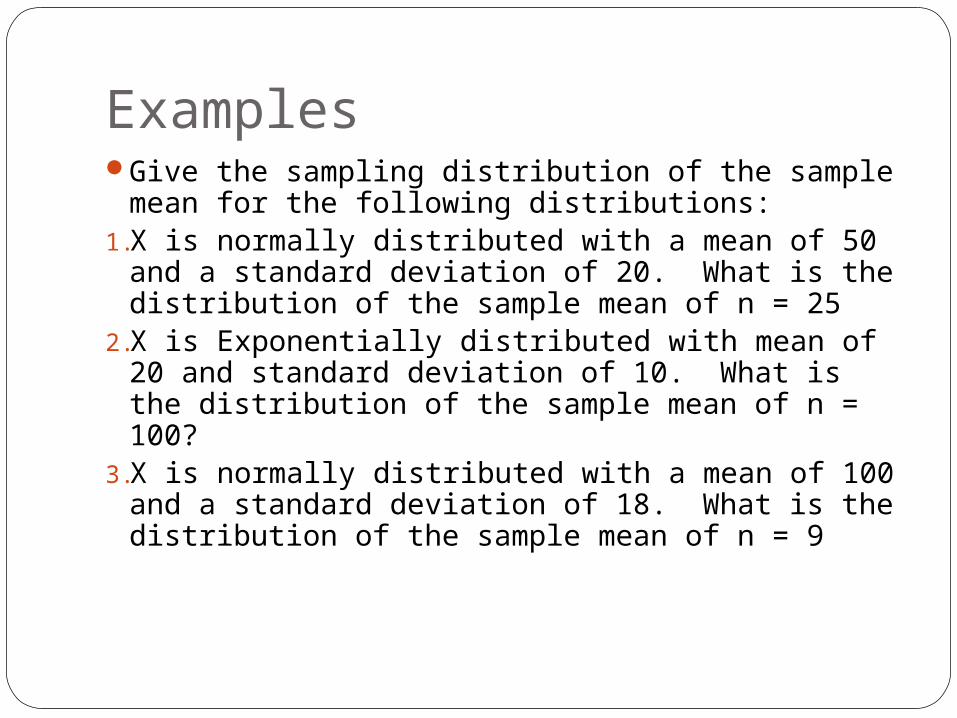
ExamplesGive the sampling distribution of the sample

mean for the following distributions:1.X is normally distributed with a mean of 50 and

a standard deviation of 20. What is the distribution of the sample mean of n = 25

2.X is Exponentially distributed with mean of 20 and standard deviation of 10. What is the distribution of the sample mean of n = 100?

3.X is normally distributed with a mean of 100 and a standard deviation of 18. What is the distribution of the sample mean of n = 9

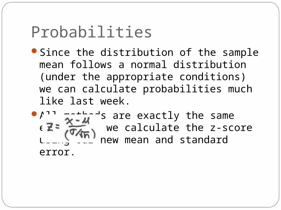
ProbabilitiesSince the distribution of the sample mean

follows a normal distribution (under the appropriate conditions) we can calculate probabilities much like last week.

All methods are exactly the same except now we calculate the z-score using our new mean and standard error.

Example: Back to SAT ScoresFrom last week we said that SAT Math Scores

are Normally distributed with a mean of 500 and a standard deviation of 100.

X~N(500,100)What is the sampling distribution of the

sample mean of a class of 25 students?What is the probability that A RANDOMLY

SELECTED STUDENT scores above a 600 on the SAT Math section?

What is the probability that THE MEAN SCORE OF THE 25 STUDENTS is above 600?

Section 8.2

Large Sample Confidence Intervals

Point EstimatorSuppose we do not know the true population mean.

How can we estimate it? We could find a sample and use a statistic such as the

sample mean to estimate it This is known as a point-estimate

But it is unlikely that our sample mean is going to exactly match the population mean even under perfect conditions

For this reason, it is better to state that we believe the true mean is between two numbers a and ba < µ < b

We can predict a and b using a confidence interval

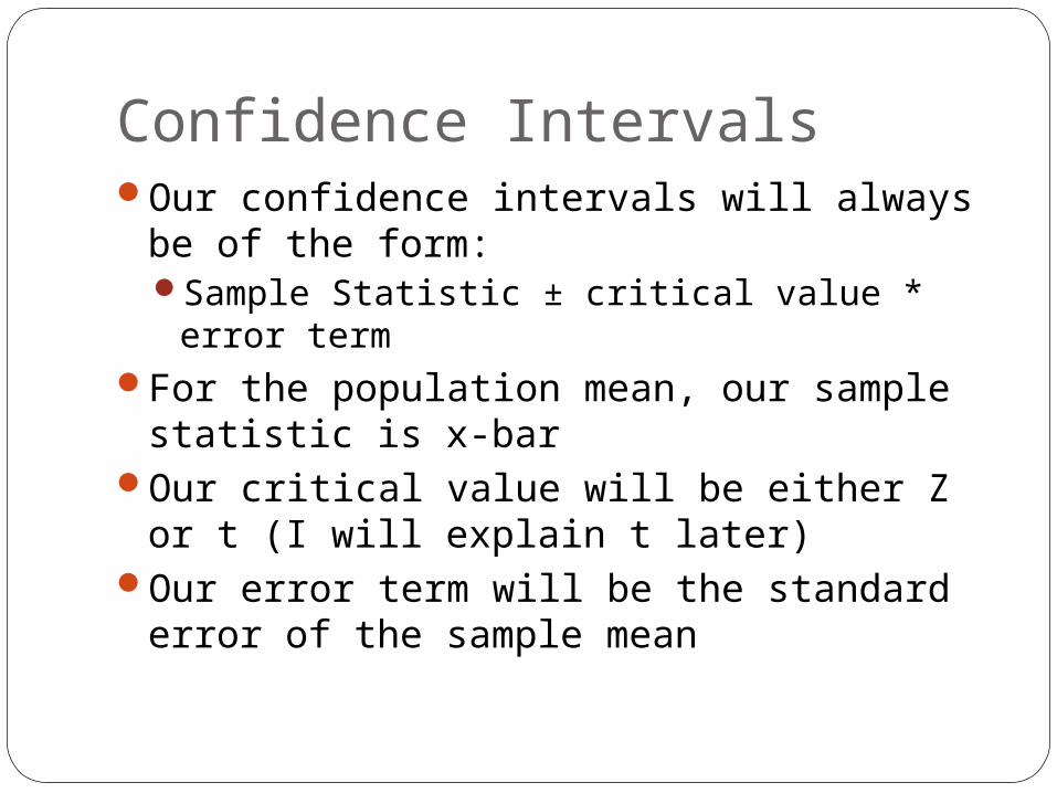
Confidence IntervalsOur confidence intervals will always be of

the form:Sample Statistic ± critical value * error term

For the population mean, our sample statistic is x-bar

Our critical value will be either Z or t (I will explain t later)

Our error term will be the standard error of the sample mean

Large Sample Confidence IntervalsRecall if n is “large” (≥20), X-bar’s dist. is

approximately normal with mean mu and standard error sigma/sqrt(n)

95% CI

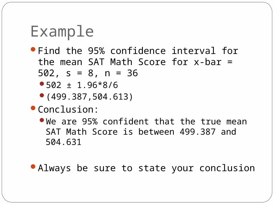
ExampleFind the 95% confidence interval for the

mean SAT Math Score for x-bar = 502, s = 8, n = 36502 ± 1.96*8/6(499.387,504.613)

Conclusion:We are 95% confident that the true mean

SAT Math Score is between 499.387 and 504.631

Always be sure to state your conclusion

Confidence LevelsIn the previous slide, we used a confidence

level of 95%.This corresponded to a critical value of 1.96

We commonly use 3 different confidence levels:

90%Critical Value of 1.645

95%Critical Value of 1.96

99%Critical Value of 2.578

Notes on the Error TermThe error term can be effected by 3 different

things1.The sample size, n

The larger n, the smaller the error term2.The standard deviation, s

The smaller s, the smaller the error term3.The confidence level

The higher the confidence level, the larger the critical value, the larger the error term

We cannot choose s in practice, but we can choose the confidence level and often n

Section 8.3

Small Sample Confidence Intervals

Small Sample Confidence IntervalsFor “large” sample sizes, we have the

convenience of knowing that the distribution approaches normalityWe can use the Z table (1.645, 1.98, 2.645)

For “small” sample sizes (<20) we have to do a little more work and we must know that X is normalOur Central Limit Theorem Rules do not apply

Two Cases1.The population standard deviation is known2.The standard deviation is unknown

Case 1: Sigma is knownGood news!In this case we handle our confidence intervals

in the exact same way we would for a large sample

Example: Compute a 99% confidence interval for the

population mean when x-bar= 43.2, sigma = 18, n = 16(31.6, 54.8)

We are 99% confident that the population mean is between 31.6 and 54.8

Case 2: Sigma is unknownWhen the population standard deviation is

unknown we need to make a slight adjustment to our formula.

The adjustment is in the critical value. Rather than using our Z values (1.645, 1.98, 2.645) we will be using t values

t values come from the t-distribution. You will only need to know the t-distribution for inference, not probability.

T-distributiont values can be found on Table FNotes about t

t is mound shaped and symmetric about the mean, 0Just like the standard normal

It looks exactly like the standard normal, except with larger tails.

The values of T require a parameter, degrees of freedom, to find the value on the tableDegrees of freedom are equal to n – 1

As n increases, t approaches Z

ExampleConstruct a 95% confidence interval for the

mean weight of apples (in grams):x-bar = 183, s = 14.1, n = 16First find t

Alpha/2 = .025 ( because of 95% confidence)df = n-1 = 15t = 2.13

183±2.13*14.1/sqrt(16)(175.5 and 190.5)We are 95% confident that the mean weight

of apples is between 175.5 and 190.5 grams