137

CENTER PIVOT EVALUATION AND DESIGN

Dale F. HeermannAgricultural Engineer

USDA-ARS2150 Centre Avenue, Building D, Suite 320

Fort Collins, CO 80526Voice -970-492-7410 Fax - 970-492-7408

Email - dale.heermann@ars.usda.gov

INTRODUCTION

The Center Pivot Evaluation and Design Program (CPED) is a simulation model. It is based on the first model presented by Heermann and Hein (1968) which wasverified with field data. Their simulation model required input of the sprinklerlocation, discharge, pattern radius and an assumed stationary pattern shape ofeither triangular or elliptical. The application depth versus distance along a radialline from the pivot was determined and application rates at a specified distancefrom the pivot were determined. The hours per revolution were input and eachtower was assumed to move at a constant speed for the complete circle. Kincaid,Heermann and Kruse (1969) used the model to calculate potential runoff fordifferent system capacities and infiltration rates. Kincaid and Heermann (1970)added the calculation of the flow resistance and verified with measured pressuredistribution along the center pivot lateral. Chu and Moe (1972) studied thehydraulics of a center pivot system and developed a quick approximation fordetermining the pressure loss from the pivot to the outer end of the lateral as aconstant (0.543) times the loss that would occur if the entire discharge flowed thetotal length of the lateral.

The model was adapted by Beccard and Heermann (1981) to include the effect oftopographic differences in the resulting application depths along radii of the centerpivot in non level fields. The model included the pump and well characteristicsand calculated the hydraulic equilibrium point as the system moved to differentpositions on a rough terrain. The model was exercised to determine the uniformitychanges when converting from high pressure to low pressure on rough terrain. Edling (1979), and James (1984) also used simulation models to study theperformance of center pivot systems on variable topography and with differentpressures.

138

The current simulation model has been expanded to include donut shapedstationary patterns that can be used to represent many of the low pressure sprayheads. The start-stop of the electric motors and the speed variation in hydraulicdrives can also effect the uniformity in the direction of travel (Heermann and Stahl,1986). The input of the start-stop sequence for each tower replaces theassumption of a constant speed and the variability of application depths in thedirection of travel has been simulated.

EXAMPLES OF SIMULATION EVALUATION

The uniformity of application depths can be calculated by inventorying the sprinklerhead models, nozzles sizes and distance from the pivot. The pump curve anddrawdown, or pivot pressure, or discharge is also needed. Figure 1 illustrates asimulation as designed and the distribution if the sprinkler heads were reversedbetween 2 towers made at the time of installation. The application rate andpotential runoff are illustrated in Figure 2. Figure 1. Typical center pivot as designed (CU = 90.8) and with 10 sprinklerheads incorrectly installed shown as a dashed line (CU = 87.9).

139

Figure 2 Example application rate curve versus 0.5 and 1.0 SCS intake curve.

EVALUATION OBJECTIVES

The selection or development of an evaluation standard and procedures shouldfocus on the need for the evaluation. The USDA, Environmental Quality IncentiveProgram (EQIP) administered by the Natural Resource Conservation Service(NRCS) currently can provide cost sharing on the installation and upgrading ofirrigation systems for improving water quality or conservation under irrigation. Center pivots are frequently the system of choice. There is a need to assure thatinstalled systems will provide the desired improvement in irrigation performance. A similar need exists for any user of center pivot systems to assure that aninstalled or modified system will perform as designed. It must be recognized thatthe scheduling of irrigations is most important for the beneficial use of water. Efficient scheduling of irrigation systems requires knowing the amount of waterapplied per irrigation. The CPED program has been streamlined and simplified foruse in evaluating center pivot systems for cost sharing on new and upgradedsystems. The CPEDLite program is similar to the one being used in thisworkshop. The primary difference is the simulations are for 1 foot intervalsbeginning and ending at fixed distances. This assures that any simulation willprovide the same results. The uniformity is output in 5% bands.

140

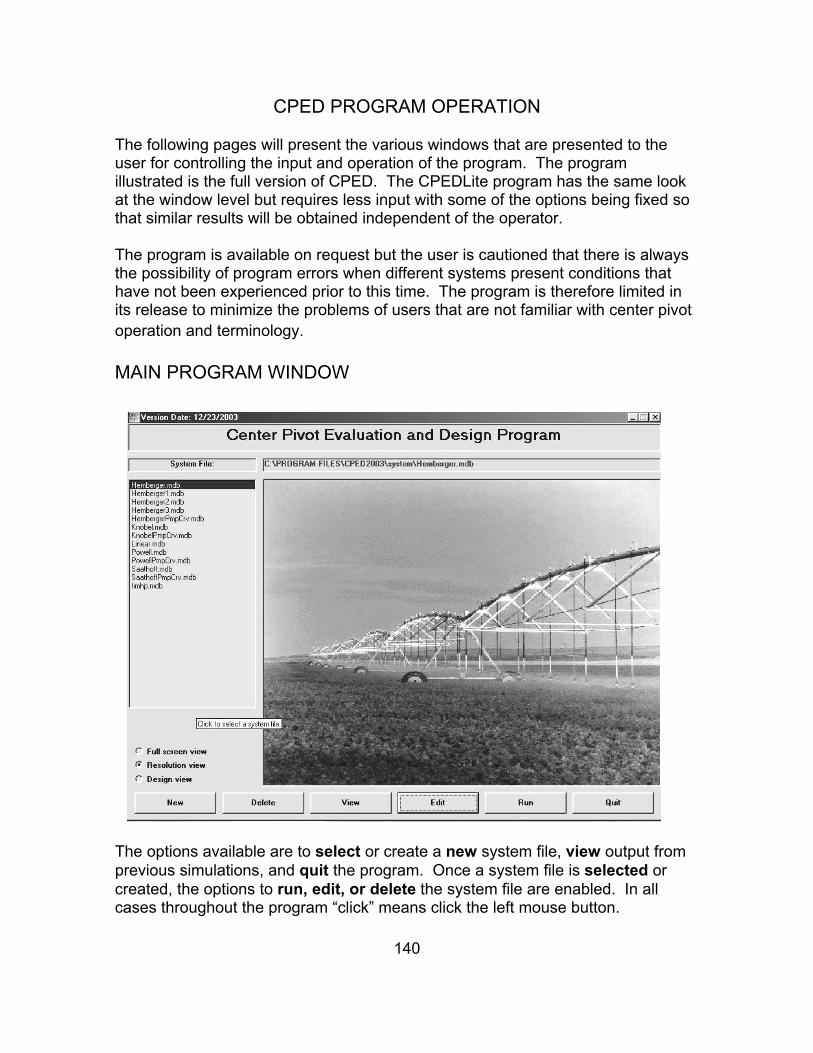
CPED PROGRAM OPERATION

The following pages will present the various windows that are presented to theuser for controlling the input and operation of the program. The programillustrated is the full version of CPED. The CPEDLite program has the same lookat the window level but requires less input with some of the options being fixed sothat similar results will be obtained independent of the operator.

The program is available on request but the user is cautioned that there is alwaysthe possibility of program errors when different systems present conditions thathave not been experienced prior to this time. The program is therefore limited inits release to minimize the problems of users that are not familiar with center pivotoperation and terminology.

MAIN PROGRAM WINDOW

The options available are to select or create a new system file, view output fromprevious simulations, and quit the program. Once a system file is selected orcreated, the options to run, edit, or delete the system file are enabled. In allcases throughout the program “click” means click the left mouse button.

141

A system file can be Selected by clicking one of the systems listed in the list boxlabeled System File List. The name of the selected system file will be displayed inthe label box labeled Name of Selected System File.The New button allows the user to create a new system file. There are two waysto create a new system. The first way is to enter a name and click the OK button. You are then transferred into the Edit window that is discussed below. Thesecond option is to create a system from an existing file. You then select theexisting file; name the new system; click the OK button and you will be in the Editwindow where only changes need to be entered.

The Delete button will delete the selected system file from the user’s hard drive.The user will be asked for confirmation before deleting a system file.

The View button allows examining previous simulation results. The View previousoutput button will bring up the data files that have been saved from previoussimulations. Selecting one of these files will plot to the screen the simulated depthversus distance data.

The Analyze catch can data button allows you to enter catch can data foruniformity evaluation. A simulation output data set can be input to the catch candata file and allow the uniformity analysis for different distances along the lateral.The procedure to save simulation data is presented latter with running theprogram.

The Edit button allows editing of the selected system file. More detail is below.

The Run button moves to the screen for entering the parameters to run the simulation. More detail is given below.

The Quit button exits the program. Pressing CTRL +Q anytime during thesimulation will have the same effect.

EDIT SYSTEM FILE WINDOW

The different information groups of data can be entered or edited by moving themouse pointer over the image of the sprinkler system. The labels PumpInformation, Tower Information, Sprinkler Information, Span Information, andSystem Information can be selected by clicking on the text to open its edit window.

The Add/Edit Sprinkler Model button opens a window for adding or editingsprinkler models. This is password protected and normally is not needed by theuser. Those supporting the program will do this editing. The Previous Windowbutton saves the changes and returns to the main program window.

142

SPRINKLER EDIT WINDOW

143

Figure 3. Part circle sprinklers angles. Angles arebetween 0 -180 degrees with an L or R prefix.

A new sprinkler can be added by clicking the Add Sprinkler button. If no sprinklers arepresent by pressing the Add Sprinkler button a sprinkler with zero distance will defaultand you can begin by entering the other information for the first sprinkler. The sprinklermodel is selected by clicking on the model listed in the box labeled Sprinkler Model List.Sprinklers can be added in any order. If one sprinkler is missed you can merely add itat any time. By clicking the Reorder Sprinklers button the sprinklers will be orderedfrom the pivot to the outer end based on their individual distances from the pivot. Youdo not enter the sprinkler number as this is done automatically. If sprinklers are presentthe information from the previous record will be used and the distance will automaticallybe incremented. Edit the information for the newly added sprinkler. Many systems willhave the same sprinkler models and these will need no editing. If the sprinkler spacingis uniform this will also require minimal editing. Even the nozzle sizes may be the samefor several sprinklers minimizing the editing required.

The nozzle size is the diameter in 1/64 inches. For example a nozzle diameter of 9.5 isequal to 9.5/64 or 19/128 inch. There are columns for a range and spread nozzlewhich was typical for high pressure heads. Enter the diameter for single nozzlesprinklers in the range column. The pressure control column is the outlet pressure ofthe pressure regulator if this is selected in the System file screen. When the constantorifice is the selected pressure control, the orifice size in 64th inch is entered. When thiscolumn is left blank, it is an indication there is no flow control on that sprinkler even ifthe system has pressure regulation selected.

The start and stop angles are viewed from the pivot toward a part circle sprinkler. Check if the sprinkler starts on the right or left. Then using the pipe as the zeroreference point, measure the angle back toward the pivot. Use the same technique forthe stop angle. All angles are positive and between 0 and 180 degrees (Figure 3).

144

Alternatively you can move to the bottom row marked with an '*' and enter the newsprinkler information manually. A sprinkler can be deleted by selecting any column inthe row for the sprinkler and click the Delete button.

The Reorder button will sort and number the sprinklers by sprinkler distance from thepivot.

The Previous Screen button returns to the Edit system file window.

TOWER EDIT WINDOW

Towers are added by clicking on the Add Tower button and editing the distance from thepivot and its elevation. It is often assumed that the pivot and all towers are at anelevation of 100 feet if no field information is available. For the linear system, the firstcart is assumed to be the pivot with a distance of 0. As the Add Tower button is clicked,the towers are added with the spacing of the previous two towers and the sameelevation as the previous tower. The Reorder Towers will sort the towers by distancefrom the pivot if there happen to be entered in the wrong sequence. Select a tower andclick the Delete Tower button if a tower needs to be deleted. The Previous Screenreturns to the Edit system file window.

145

SPAN INFORMATION WINDOW

Clicking the Add Span button inserts a starting distance of 0 and the Pipe I.D. and theDarcy-Weisbach resistance coefficient must be entered. A typical value of the D-Wcoefficient is 0.xxx to 0.xxx for center pivots. Multiple pipe sizes can be added byclicking the Add Span button and entering the starting distance from the pivot and itsresistance coefficient. The spans are assumed to go from the starting distance to thenext span or end of the pivot for the last span. Spans can be deleted (Delete Span) and reordered (Reorder spans) by clicking the appropriate button. Never delete thespan with starting distance of 0. The Previous Screen button returns to the Edit systemfile window.

PUMP INFORMATION WINDOW

The piping to the pivot, pump curve, and pivot elevation are entered in this window. Ifthe pump curve information is not available, either a constant discharge or constantpressure can be selected.

146

Selecting the Normal option requires the quadratic equation for the pump curve. Thecurve of the total head vs discharge for the pump is needed to develop the regressionequation that describes the pump. This relationship can be determined externally fromthis program or there is an option that will fit the pump curve equation with points from apump curve or field measured data. At least 4 points that span the operating range areneeded, however 8-10 will give a better fit. Problems have occurred where theoperating point is beyond the pump curve data. Use caution. The form of the equationfor the pump curve is:

Q = B0 + B1H + B2H2

where:Q - discharge - gpmH - head/stage - psiB0 - interceptB1 - linear slope coefficient on headB2 - quadratic slope coefficient on head

The number of stages for the pump must be entered when the manufacturers pumpcurve is for a single stage. However, if the pump curve comes from fieldmeasurements, set the number of stages equal to one. The Calculate Pump Curvebutton can be selected for calculating the coefficients when data are available from

147

either the manufacturers pump curve or field measured data. The paired data ofdischarge in gpm and head in feet can be entered and the three coefficients calculated.

The total dynamic lift in feet must also be entered. It is the elevation difference (feet)between the center pivot pad elevation and the depth to the water table including thedrawdown while pumping. The pad elevation is the elevation for the center pivot at froman assumed or measured datum elevation. The sprinkler height is the distance abovethe pad height for the sprinklers as if they were on a level field. The inside diameter(I.D.) of the pipe size and length of pipe from the pump to the pivot and the I.D. of theriser pipe must be entered. Include the Darcy-Weisbach coefficient for both pipes.

The Constant Head option is where the pivot pressure (psi) is specified. This is themost stable option where the pump curve is not known. Estimate the discharge in gpmand set the number of stages equal to one. The estimate discharge is only to shortenthe calculation time and the actual value is not critical.

The Constant Discharge in gpm can also be specified. The potential problem withconstant discharge is when all sprinklers are regulated. If the discharge does not matchthe calculated discharge with the regulated pressure an error will occur when attemptingto have the calculated discharge on the system match that specified. Again set thenumber of stages equal to one.

The constant head and constant discharge does not require pump to riser pipe and riserpipe sizes or resistance coefficient since the pressure or discharge is assumed to be atthe pivot and no head loss is calculated for these sections. The Previous Screen buttonreturns to the Edit system file window.

SYSTEM INFORMATION SCREEN

Three options for the Type of Pressure Control can be select from the drop down box. They are none, pressure regulated, or constant orifice. Systems with booster pumps forthe big gun at the end of a center pivot system are simply estimated with a pressureincrease in psi just prior to the big gun or guns. The number of sprinklers beyond thebooster pump is specified. The actual pressure is dependent on the center pivot systemand the inlet pressure, discharge or pump curve.

The Previous Screen button returns the Edit system file window.

148

RUN WINDOW

149

This is the screen that you will enter when you click RUN and all of the system files withthe necessary data have been entered. Minimal input is required on this screen beforethe simulation is run. The Default button will restore the default values that were usedon the previous simulation run for this system. The hours/revolution are entered toobtain the depth for this condition. Normally the sprinkler number is set to “all” forincluding all the sprinklers to be simulated. However, you can select one sprinkler byentering its number to see the contribution to the depths from the specified sprinkler.

The start, stop distances and distance increment specifies the location for simulationdepths. For example you can start at 10 feet and go to 500 feet with 5 foot increments. The minimum depth specifies that only locations with depths greater than that will beincluded in the uniformity calculations. This is often desirable when not including thesmall depths at the outer boundary where there is not sufficient overlap with othersprinklers. The CPEDLite program fixes these four parameters and only the speed inhours/revolution can be changed.

Clicking the RUN button will start the simulation. You will automatically be moved toanother window that will plot the simulated depth versus distance data on the monitor. Prior to pressing RUN you can select a catch can data set or data saved from aprevious run to be displayed on the monitor after the simulation is completed. Thisprovides a visual comparison of the current simulation with other data. The data forcomparison can be selected from the files listed in the Catch Can File Window. ThePrevious Screen button will return to the Main Window.

You will note a possible selection to Adjust output graph to starting distance. This isnormally not needed when simulating the entire system. Clicking this selection isbeneficial if you are not simulating from near the pivot and want the plot to begin at thestarting distance instead of 0.

SIMULATION OUTPUT WINDOW

The output window plots the simulated depth versus distance from the pivot for theparameters set in the run window. The Coefficient of Uniformity, the DistributionUniformity, and mean application depth are printed. The Q-Depths, gpm, is thedischarge calculated from all simulated depths while the Effective Q-Depths, gpm, iscalculated from the depths that are above the specified minimum depth used in theUniformity and mean depth calculations. The effective area is the simulated area forthose areas receiving more than the minimum depth between the starting and stopdistances. The window below is an example of plotting catch can data from a previoussimulation run.

Additional data can be printed either to the printer or to a file. The Return to Main Menubutton will return to the main menu screen. The Print to File button will ask for the filename for storing the information. You will then be prompted for saving the individual

150

sprinkler and tower data followed for a prompt to save the simulated depth data and the name for its file. The saved simulated depth data are then availablefor comparison with future simulations for the same center pivot system.

The following information can be printed to the printer after the simulation run.1. The head per stage of the pump - gpm2. The pivot pressure - psi3. The system discharge based on the pump curve - gpm4. The system discharge based on all the integrated depths - gpm 5. The system discharge based on all depths above the minimum depth - gpm6. The effective irrigated area, which is the area receiving water above the minimum

depth - acres7. The mean depth - in. (of all depths above the minimum)8. Christiansen's uniformity coefficient (of all depths above the minimum)9. Mean low quarter uniformity (of all depths above the minimum)10. Plot of depth vs distance

The information that is available for each sprinkler is the line pressure - psi, the nozzlepressure - psi, the discharge - gpm, and the pattern radius - ft.

151

The application depths are the final piece of information provided. They are listed bydistance.

The Previous Window button saves the changes to the system file and returns to themain program window.The Previous Window button saves the changes to the systemfile and returns to the main program window.

REFERENCES

Beccard, R. W. and D. F. Heermann. 1981. Performance of pumping plant--centerpivot sprinkler irrigation systems. ASAE Paper 81-2548, Chicago, IL. Chu, T.S. and D.L. Moe. 1972. Hydraulics of a center pivot system. Trans. of theASAE 15(5):894,896.

Edling, R.J. 1979. Variation of center pivot operation with field slope. Trans. of ASAE15(5):1039-1043.

Heermann, D. F. and P. R. Hein. 1968. Performance characteristics of theself-propelled center pivot sprinkler irrigation system. Trans. ASAE 11(1):11-15.

Heermann, D.F. and K.M. Stahl. l986. Center pivot uniformity for chemigation. ASAEPaper 86-2584, Chicago, IL.

James, L.G. 1984. Effects of pump selection and terrain of center pivot performance. Trans. of ASAE 27(1):64-68,72.

Kincaid, D. C., D. F. Heermann and E. G. Kruse. 1969. Application rates and runoff incenter pivot sprinkler irrigation. Trans. ASAE 12:790-794, 797.

Kincaid, D. C. and D. F. Heermann. 1970. Pressure distribution on a center pivotsprinkler irrigation system. Trans. ASAE 13:556-558.