AEGON Asset Management Olaf van den Heuvel Head of Tactical Asset Allocation CFA Forecasting dinner.

Daily prostate positioning
Frank Van den Heuvel Ph.D.
Lei Dong Ph.D.
David Jaffray Ph.D.
27th July 2004

• Measure with a micrometer.

• Measure with a micrometer.
• Mark with chalk.

• Measure with a micrometer.
• Mark with chalk.
• Cut with an axe.

• Measure with a micrometer.
• Mark with chalk.
• Cut with an scalpel.
Now that we have IMRT.
• Measure with a micrometer.
• Mark with chalk.
• Cut with an scalpel.
Now that we have IMRT.
But, we are very precise in determining the thickness of our
chalk!
The Goal of Image Guided Radiation Treatment

The Goal of Image Guided Radiation Treatment
Reduction of the PTV margin!

The Goal of Image Guided Radiation Treatment
Reduction of the PTV margin!
The PTV margin depends on:
• Organ
• Patient
• Modality of Treatment

van Herk et al.[1] proposes a margin recipe, based on:

van Herk et al.[1] proposes a margin recipe, based on:
• Obtaining a 98% equivalent uniform dose (EUD)

van Herk et al.[1] proposes a margin recipe, based on:
• Obtaining a 98% equivalent uniform dose (EUD)
• For 90% of the patients

van Herk et al.[1] proposes a margin recipe, based on:
• Obtaining a 98% equivalent uniform dose (EUD)
• For 90% of the patients
• Calculate this using a simulation procedure, using MC
calculations to simulate population spread.
Recipe:
M = 2.5Σ + 0.7σ − 3mm

van Herk et al.[1] proposes a margin recipe, based on:
• Obtaining a 98% equivalent uniform dose (EUD)
• For 90% of the patients
• Calculate this using a simulation procedure, using MC
calculations to simulate population spread.
Recipe:
M = 2.5Σ + 0.7σ − 3mm
• Σ: Spread of the systematic errors SD(Σi)
• σ: Average of the random errors < σi >

Reducing the Margin

Reducing the Margin
We can reduce Σ and/or σ

Reducing the Margin
We can reduce Σ and/or σ
Reduction of Σ is most efficient and easiest to do

Reducing the Margin
We can reduce Σ and/or σ
Reduction of Σ is most efficient and easiest to do
Off Line Is the most popular correction system, to
date.
1. Gather data to sample positional distribution (up to
six fractions).
2. Apply a correction to minimize the systematic error.
3. Adapt margins to reflect the variations.

On–line adjustment: reduces both Σ and σ at
the same time.
1. No “bad” treatments
2. Conceptually simple, no assumptions on type of
probability distributions
How[2]
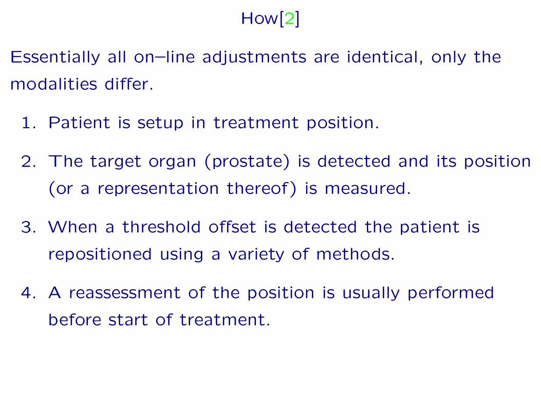
Essentially all on–line adjustments are identical, only the
modalities differ.
1. Patient is setup in treatment position.
2. The target organ (prostate) is detected and its position
(or a representation thereof) is measured.
3. When a threshold offset is detected the patient is
repositioned using a variety of methods.
4. A reassessment of the position is usually performed
before start of treatment.

On-line adjustment modalities
• Ultrasound detection
• Implanted Markers
– Active
– Passive
∗ US
∗ EPID
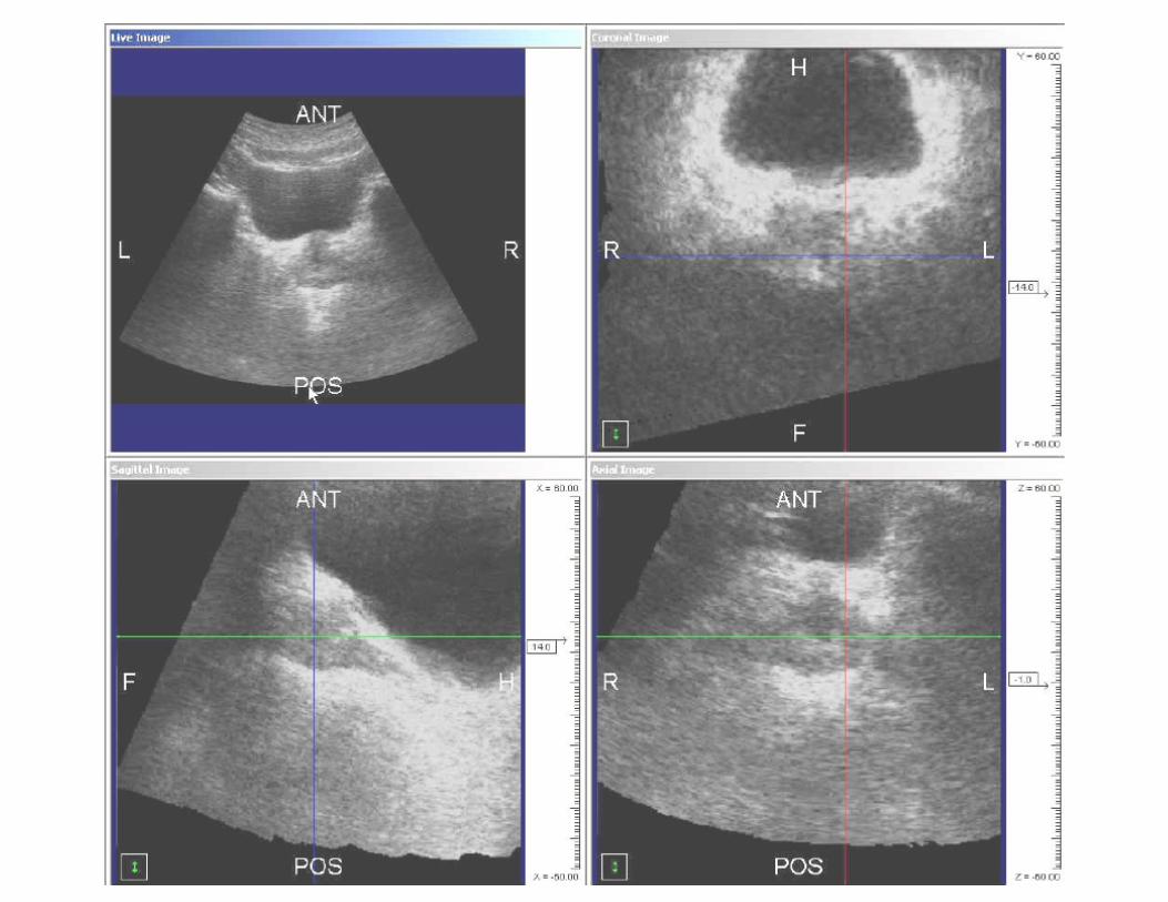
Ultrasound adjustment


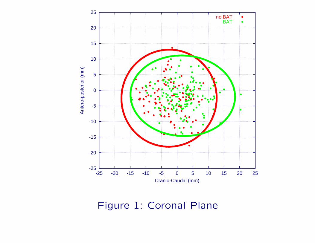
Verification of Ultrasound based adjustment[3]
• A total of 19 patients have been enrolled.
• Compiled data of 17 patients will be presented.
• 275 treatment setups with markers have been analyzed.
• 156 image pairs using Ultrasound adjustment.
• 119 image pairs using traditional treatment.
-25
-20
-15
-10
-5
0
5
10
15
20
25
-25 -20 -15 -10 -5 0 5 10 15 20 25
Ant
ero-
post
erio
r (m
m)
Cranio-Caudal (mm)
no BATBAT
Figure 1: Coronal Plane
-25
-20
-15
-10
-5
0
5
10
15
20
25
-25 -20 -15 -10 -5 0 5 10 15 20 25
Cra
nio-
caud
al (
GT
is p
ositi
ve)
(mm
)�
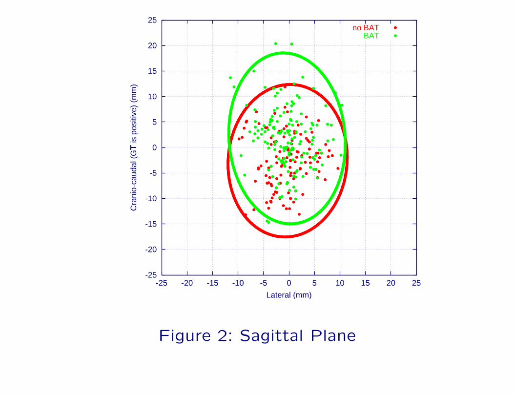
Lateral (mm)
no BATBAT
Figure 2: Sagittal Plane

-25
-20
-15
-10
-5
0
5
10
15
20
25
-25 -20 -15 -10 -5 0 5 10 15 20 25
Ant
ero-
post
erio
r (U
p is
pos
itive
) (m
m)
�
Lateral (mm)
no BATBAT
Figure 3: Transverse plane

Why doesn’t Ultrasound aided repositioning perform better?

Why doesn’t Ultrasound aided repositioning perform better?
• User subjectivity[4].

Why doesn’t Ultrasound aided repositioning perform better?
• User subjectivity[4].
• Discrepancy between contoured anatomy and actual
anatomy[5].

Figure 4: Inter–observer variation of contouring bladder

Why doesn’t Ultrasound aided repositioning perform better?
• User subjectivity[4].
• Discrepancy between contoured anatomy and actual
anatomy[5].
• Intra–fractional movement between the Ultrasound
procedure and the treatment[6].
Why doesn’t Ultrasound aided repositioning perform better?
• User subjectivity[4].
• Discrepancy between contoured anatomy and actual
anatomy[5].
• Intra–fractional movement between the Ultrasound
procedure and the treatment[6].
• Heisenberg ∆x∆p > h̄2

Improvements to reduce User subjectivity

Improvements to reduce User subjectivity
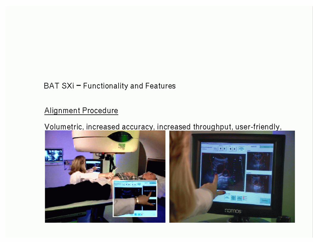
1. BAT (Nomos Inc)
• Live CT–contour projection during acquisition.
• Seed localizers (Visicoil, Radiomed)

Improvements to reduce User subjectivity
1. BAT (Nomos Inc)
• Live CT–contour projection during acquisition.
• Seed localizers (Visicoil, Radiomed)
2. Zmed (Varian Inc)
• Pseudo 3D acquisition.
• Live adjustment.


Improvements to reduce User subjectivity
1. BAT (Nomos Inc)
• Live CT–contour projection during acquisition.
• Seed localizers (Visicoil, Radiomed)
2. Zmed (Varian Inc)
• Pseudo 3D acquisition.
• Live adjustment.
3. IBeam (CMS Inc)
• Pseudo 3D acquisition and reconstruction.
• Ultrasound contouring and export to planning
system.

Marker based protocols


Marker based protocols
Ultrasound Do not look for prostate, but look for long
seeds (need 3D acquisition)
EPID Take images and visualize the seeds
Calypso Seeds reflect RF radiation use detector to see
where they are.


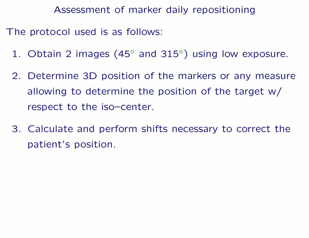
Assessment of marker daily repositioning
The protocol used is as follows:
1. Obtain 2 images (45◦ and 315◦) using low exposure.

Assessment of marker daily repositioning
The protocol used is as follows:
1. Obtain 2 images (45◦ and 315◦) using low exposure.
2. Determine 3D position of the markers or any measure
allowing to determine the position of the target w/
respect to the iso–center.
Assessment of marker daily repositioning
The protocol used is as follows:
1. Obtain 2 images (45◦ and 315◦) using low exposure.
2. Determine 3D position of the markers or any measure
allowing to determine the position of the target w/
respect to the iso–center.
3. Calculate and perform shifts necessary to correct the
patient’s position.


Results
An IRB approved study with 15 patients total accrual
(currently 14 accrued) was initiated, using the
abovementioned protocol.

Results
An IRB approved study with 15 patients total accrual
(currently 14 accrued) was initiated, using the
abovementioned protocol.
Results shown here are for 10 patients. A total of 270
treatments were analyzed (27 fractions average per
patient).
Results
An IRB approved study with 15 patients total accrual
(currently 14 accrued) was initiated, using the
abovementioned protocol.
Results shown here are for 10 patients. A total of 270
treatments were analyzed (27 fractions average per
patient).
Every fraction had before and after measurements.
Resulting in 540 total position measurements (270 before
and after pairs).

mean (mm) SD (mm)
before
AP 7.45 5.99
LAT 1.29 5.34
CC 5.12 4.44
after
AP 0.65(P < 0.00001) 2.82(P < 0.00001)
LAT 0.11(P < 0.00001) 2.64(P < 0.00001)
CC 0.46(P < 0.00001) 2.22(P < 0.00001)
Table 1: Pooled results, significance of reduction using t–
test(mean) and F–test(Variances)

-30
-20
-10
0
10
20
30
-30 -20 -10 0 10 20 30
AP
(m
m)
CC (mm)
AfterBefore
Figure 5: Scatterplot showing before and after positions for a total of 540 mea-surements. All sizes are in millimeter. The ellipses cover 95% of all datapoints.

Margin Calculations
Σ (mm) σ (mm) Margin (mm)
before
AP 3.6 5.08 9.6
LAT 3.41 4.29 8.5
CC 3.88 2.36 8.4
after
AP 0.56 2.64
LAT 0.39 2.37
CC 0.40 1.95
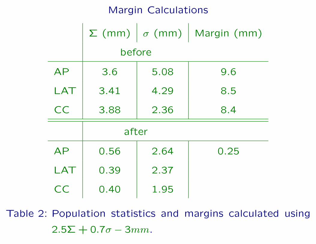
Table 2: Population statistics and margins calculated using
2.5Σ + 0.7σ − 3mm.
Margin Calculations
Σ (mm) σ (mm) Margin (mm)
before
AP 3.6 5.08 9.6
LAT 3.41 4.29 8.5
CC 3.88 2.36 8.4
after
AP 0.56 2.64 0.25
LAT 0.39 2.37
CC 0.40 1.95
Table 2: Population statistics and margins calculated using
2.5Σ + 0.7σ − 3mm.

Margin Calculations
Σ (mm) σ (mm) Margin (mm)
before
AP 3.6 5.08 9.6
LAT 3.41 4.29 8.5
CC 3.88 2.36 8.4
after
AP 0.56 2.64 0.25
LAT 0.39 2.37 -0.63
CC 0.40 1.95
Table 2: Population statistics and margins calculated using
2.5Σ + 0.7σ − 3mm.

Margin Calculations
Σ (mm) σ (mm) Margin (mm)
before
AP 3.6 5.08 9.6
LAT 3.41 4.29 8.5
CC 3.88 2.36 8.4
after
AP 0.56 2.64 0.25
LAT 0.39 2.37 -0.63
CC 0.40 1.95 -0.64
Table 2: Population statistics and margins calculated using
2.5Σ + 0.7σ − 3mm.
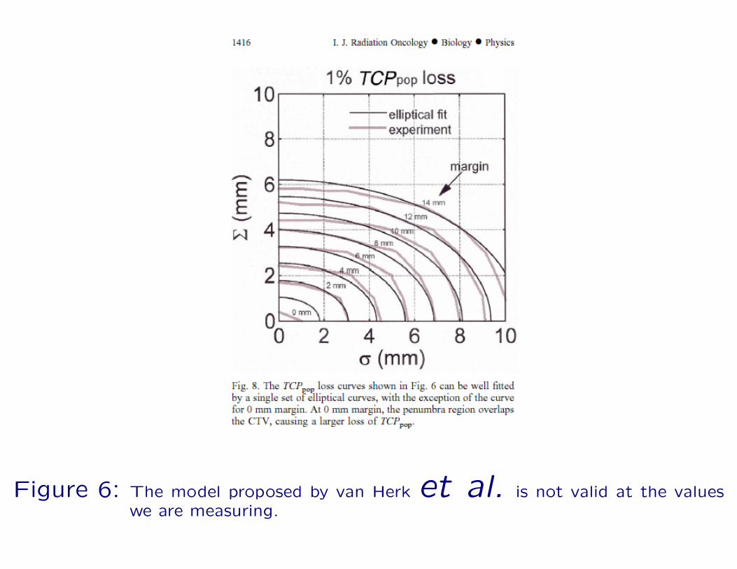
Figure 6: The model proposed by van Herk et al. is not valid at the valueswe are measuring.

Important!
Important!
The residual errors observed were after the adjustment, but
before the treatment. In order to gauge the efficacy of any
repositioning scheme we need data during the treatment.

Important!
The residual errors observed were after the adjustment, but
before the treatment. In order to gauge the efficacy of any
repositioning scheme we need data during the treatment.
We need to address the following problems:
• Patient position at time of treatment (not before or
after).
• Treatment delivery.

Important!
Important!
There are only two modalities that allow in–treatment
patient monitoring.
• EPID
• Calypso
They need to address the following problems:
• Patient position at time of treatment (not before or
after).
• Treatment delivery.
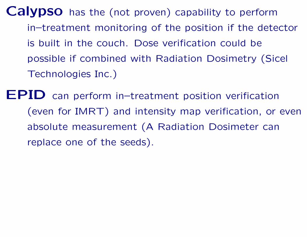
Calypso has the (not proven) capability to perform
in–treatment monitoring of the position if the detector
is built in the couch. Dose verification could be
possible if combined with Radiation Dosimetry (Sicel
Technologies Inc.)
EPID can perform in–treatment position verification
(even for IMRT) and intensity map verification, or even
absolute measurement (A Radiation Dosimeter can
replace one of the seeds).

Figure 7: Portal Image of an IMRT treatment

The previous image was taken using an electronic portal
imager in cumulative mode (e.g. All frames taken are
averaged).

The previous image was taken using an electronic portal
imager in cumulative mode (e.g. All frames taken are
averaged).
Intensity Modulation This information shows up
as fairly large variations in contrast (steps are at least
5%).
Patient Anatomy Small signals indicating bony
edges or implanted markers.
Other stuff Scattered radiation, source variations, (in
short things we don’t want to see).

32000
32500
33000
33500
34000
34500
35000
35500
36000
0 50 100 150 200 250
Pix
elV
alue
(ar
bitr
ary
units
)
Pixel Number
Patient ImageOpenImage
Figure 8: Cross–section of two images. One obtained during an IMRT–treatment(bottom) with the patient in place, the second without the patient (top).The major difference between the two signals is due to increased scat-tered radiation reaching the imager and decreased direct signal throughpatient attenuation of the primary dose.
35100
35150
35200
35250
35300
35350
35400
35450
35500
35550
0 50 100 150 200 250 300 350
Imag
er r
espo
nse
(arb
itrar
y un
its)
Pixel number
Imageadjusted open field
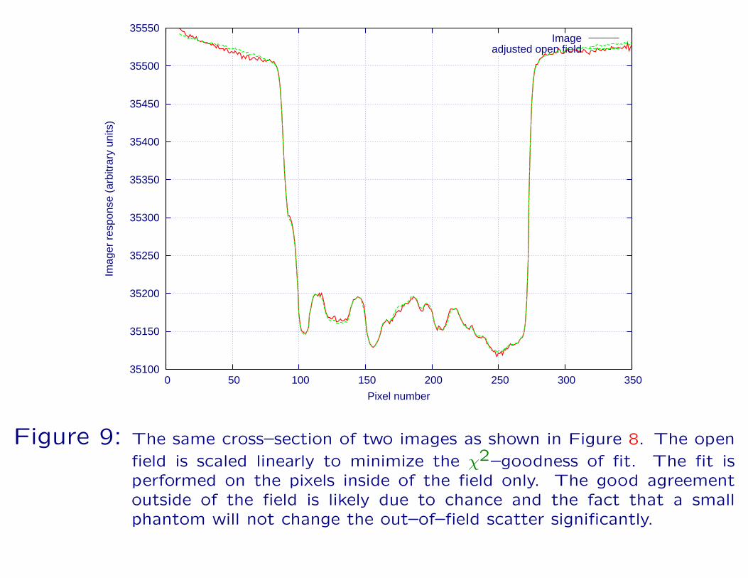
Figure 9: The same cross–section of two images as shown in Figure 8. The open
field is scaled linearly to minimize the χ2–goodness of fit. The fit isperformed on the pixels inside of the field only. The good agreementoutside of the field is likely due to chance and the fact that a smallphantom will not change the out–of–field scatter significantly.

(a) Treatment
Field
(b) Open Field (c) Subtracted
Figure 10: Two–parameter adaptive subtraction, using identical image geometry.An open image was obtained using the intensity map, the phantomplaced on the table was positioned in the beam and a new images wasacquired.

Practical application
1. Detect the field outline.
2. Adjust magnification and position of open field to
match the original portal image.
3. Mathematical morphological erosion (to stay within the
boundaries).
4. Minimize χ2-function for all pixels within detected field.
5. Determine a and b.
6. Subtract adjusted open field from original portal image.
7. Renormalize values for display.

Figure 11: Adjusted

But wait! There’s more

But wait! There’s more
The final χ2–value is sensitive to the intensity modulation
function. If the incorrect value is used the value will be
higher than normal.

But wait! There’s more
The final χ2–value is sensitive to the intensity modulation
function. If the incorrect value is used the value will be
higher than normal.
This allows to verify intensity modulated fields, if we know
how they would interact with an electronic portal imaging
device.

Pixel i
Pixel j
Figure 12: The χ2 value is calculated along each line shown in this graphical repre-sentation. This is repeated for all pixels in the image. The “error”–mapis generated by multiplying the four values, after which thresholding isperformed. Pixels that remain highlighted indicate errors in the inten-sity map.
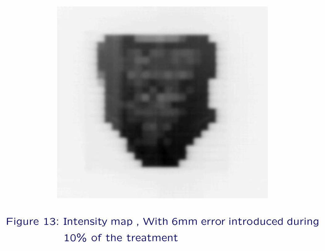
Figure 13: Intensity map , With 6mm error introduced during
10% of the treatment

Figure 14: 6mm leaf error introduced in 1 segment (10.11%
of the treatment
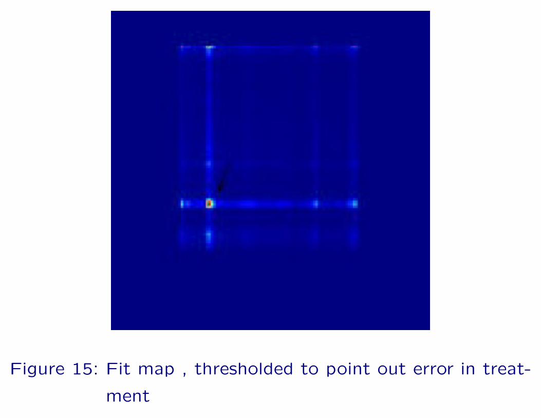
Figure 15: Fit map , thresholded to point out error in treat-
ment

Things to do
• Determine adequate threshold values (ROC analysis).
• Generate EPID-open fields.
• Can we “pre–port”?

Things to do
• Determine adequate threshold values (ROC analysis).
• Generate EPID-open fields.
• Can we “pre–port”?
Delivering a small amount of dose to the patient,
mimicking the treatment at a smaller dose rate.
Things to do
• Determine adequate threshold values (ROC analysis).
• Generate EPID-open fields.
• Can we “pre–port”?
Delivering a small amount of dose to the patient,
mimicking the treatment at a smaller dose rate.
what is an adequate pre-port amount 5MU?

Acknowledgments
• Therapists
• Jesse Larrew
• Pat McDermott
• Part of this research was sponsored by the Uniformed
Services University of the Health Sciences through
Contract No. MDA905-92-C-0009 awarded to the
Henry M. Jackson Foundation for the Advancement of
Military Medicine. The content of the information does
not necessarily reflect the position or the policy of the
government, and no official endorsement should be
inferred.
References
[1] M. van Herk, P. Remeijer, and J. V. Lebesque. Inclusion
of geometric uncertainties in treatment plan evaluation.
Int J Radiat Oncol Biol Phys, 52(5):1407–22., Apr 1
2002.
[2] F. Van den Heuvel, W. De Neve, D. Verellen, M. Coghe,
V. Coen, and G. Storme. Clinical implementation of an
objective computer-aided protocol for intervention in
intra-treatment correction using electronic portal
imaging. Radiother. Oncol., 35:232–239, 1995.
[3] Frank Van den Heuvel, Tanya Powell, Edward Seppi,
Peter Littrupp, Mubashra Khan, Yue Wang, and
Jeffrey D. Forman. Independent verification of
ultrasound based image-guided radiation tre atment,

using electronic portal imaging and implanted gold
markers. Medical Physics, 30(11):2878–2887, 2003.
[4] K. Langen, J. Pouliot, C. Azinos, M. Aubin, A.R.
Gottschalk, I. Hsu, D. Lowther, K. Shinora,
V. Weinberg, L.J. Verhey, and M. Roach. Evaluation of
the use of the bat ultrasound system for prostate
localization and repositioning: An inter–user study. Int
J Radiat Oncol Biol Phys, 54(2 Suppl):316, October
2002.
[5] G.J. Meijer, C. Rasch, P. Remeijer, and J.V. Lebesque.
Three dimensional analysis of delineation errors, setup
errors, and organ motion during radiotherapy of bladder
cancer. Int J Radiat Oncol Biol Phys, 55:1277–1287,
2003.
[6] J. Lattanzi, S. McNeeley, W. Pinover, E. Horwitz,
I. Das, T. E. Schultheiss, and G. E. Hanks. comparison
of daily localization to a daily ultrasound-based system
in prostate cancer. Int J Radiat Oncol Biol Phys,
43(4):719–25., Mar 1 1999.


![ITU - - Rob F.M. van den Brink...[2] TNO (Rob van den Brink, Bas van den Heuvel), “G.fast: The need for wideband reference models of loop segments within twisted pair cable topologies”,](https://static.fdocuments.in/doc/165x107/5f2fb83ba17d3c03f71ef55d/itu-rob-fm-van-den-brink-2-tno-rob-van-den-brink-bas-van-den-heuvel.jpg)