Climatic ChangeDOI 10.1007/s10584-016-1595-3

DADA: data assimilation for the detectionand attribution of weather and climate-related events

A. Hannart1 ·A. Carrassi2 ·M. Bocquet3 ·M. Ghil4,5 ·P. Naveau6 ·M. Pulido7 · J. Ruiz1 ·P. Tandeo8

Received: 19 March 2015 / Accepted: 3 January 2016© Springer Science+Business Media Dordrecht 2016

Abstract We describe a new approach that allows for systematic causal attribution ofweather and climate-related events, in near-real time. The method is designed so as to facil-itate its implementation at meteorological centers by relying on data and methods that areroutinely available when numerically forecasting the weather. We thus show that causalattribution can be obtained as a by-product of data assimilation procedures run on a dailybasis to update numerical weather prediction (NWP) models with new atmospheric observa-tions; hence, the proposed methodology can take advantage of the powerful computationaland observational capacity of weather forecasting centers. We explain the theoretical ratio-nale of this approach and sketch the most prominent features of a “data assimilation–baseddetection and attribution” (DADA) procedure. The proposal is illustrated in the context ofthe classical three-variable Lorenz model with additional forcing. The paper concludes by

� A. Hannartalexis.hannart@cima.fcen.uba.ar

1 IFAECI, CNRS-CONICET-UBA, Pab. II, piso 2, Ciudad Universitaria, 1428 Buenos Aires,Argentina

2 Mohn-Sverdrup Center, Nansen Environmental and Remote Sensing Center, Bergen, Norway

3 CEREA, joint laboratory Ecole des Ponts ParisTech and EDF R&D, Universite Paris-Est,Champs-sur-Marne, France

4 Ecole Normale Superieure, Paris, France

5 University of California, Los Angeles, CA, USA

6 LSCE, CNRS, Gif-sur-Yvette, France

7 Department of Physics, Universidad Nacional del Nordeste, Corrientes, Argentina

8 Telecom Bretagne, Brest, France

Climatic Change

raising several theoretical and practical questions that need to be addressed to make theproposal operational within NWP centers.

Keywords Event attribution · Data assimilation · Causality theory · Modified Lorenzmodel

1 Background and motivation

Providing causal assessments about episodes of extreme weather or unusual climate con-ditions is an important topic in the climate sciences: it arises from the multiple needs forpublic dissemination, litigation in a legal context, adaptation to climate change or simplyimprovement of the science associated with these events (Stott et al. 2013). The approachwidely used so far to was introduced one decade ago by M.R. Allen and colleagues (Allen2003; Stone and Allen 2005); it originates from best practices in epidemiology (Greenlandand Rothman 1998) and is referred to as probabilistic event attribution (PEA).

In the PEA approach, one evaluates the extent to which a given external climate forcing— such as solar irradiation, greenhouse gas (GHG) emissions, ozone or aerosol concentra-tions — has changed the probability of occurrence of an event of interest. For this purpose,one thus needs to compute two probabilities: (i) the probability of occurrence of the eventin an ensemble of model simulations representing the observed climatic conditions, whichsimulates the actual occurrence probability in the real world, referred to as factual; and (ii)the probability of occurrence of the event in a second ensemble of model simulations, rep-resenting this time the alternative world that might have occurred had the forcing of interestbeen absent, referred to as counterfactual.

Denoting by p1 and p0 the probabilities of the event occurring in the factual world andin the counterfactual world respectively, the so-called fraction of attributable risk (FAR) isthen defined:

FAR = 1 − p0

p1(1)

The FAR has long been interpreted as the fraction of the change in likelihood of an eventwhich is attributable to the external forcing. Over the past decade, most causal claims havebeen following from the FAR and its uncertainty, resulting in statements such as “It is verylikely that over half the risk of European summer temperature anomalies exceeding a thresh-old of 1.6◦C is attributable to human influence.” Stott et al. (2004). Hannart et al. (2015)have recently shown that, under realistic assumptions, the FAR may also be interpreted asthe so-called probability of necessary causation (PN) associated — in a complete and self-consistent theory of causality (Pearl 2000) — with the causal link between the forcing andthe event. The FAR thus corresponds to only one of the two facets of causality in such atheory, while the probability of sufficient causation (PS) is its second facet.

In this setting,

PN = max 1 − p0

p1, 0 (2a)

PS = max 1 − 1 − p1

1 − p0, 0 (2b)

PN = max p1 − p0, 0 (2c)

Climatic Change

where PNS is the probability of necessary and sufficient causation. Pearl (2000) providesrigorous definitions of these three concepts, as well as a detailed discussion of their mean-ings and implications. It can be seen from Eq. 2 that causal attribution requires to evaluatethe two probabilities, p0 and p1, which is therefore the central methodological question ofPEA.

So far, most case studies have used large ensembles of climate model simulations inorder to estimate p1 and p0 based on a variety of methods. However, this general approachhas a very high computational cost and is difficult to implement in a timely and sys-tematic way. As recognized by Stott et al. (2013), this remains an open problem: “theoverarching challenge for the community is to move beyond research-mode case studiesand to develop systems that can deliver regular, reliable and timely assessments in theaftermath of notable weather and climate-related events, typically in the weeks or monthsfollowing (and not many years later as is the case with some research-mode studies)”.Several research initiatives are presently addressing this real-time attribution challenge.For instance, the weather@home system (Massey et al. 2014) in the context of the WorldWeather Attribution initiative (http://www.climatecentral.org/wwa), the system proposedby Christidis et al. (2013), or the Weather Risk Attribution Forecast system (http://www.csag.uct.ac.za/∼daithi/forecast/) aim at meeting those requirements within the conventionalensemble-based approach.

The purpose of this article is to introduce a new methodological approach that addressesthe latter overarching operational challenge. Our proposal relies on a class of powerful sta-tistical methods for interfacing high-dimensional models with large observational datasets.This class of methods originates from the field of weather forecasting and is referred to asdata assimilation (DA) (Bengtsson et al. 1981; Ghil and Malanotte-Rizzoli 1991; Talagrand1997).

Section 2 explains the rationale of the approach proposed herein, presents a briefoverview of DA, and outlines the most prominent technical features of a “data assimilation–based detection and attribution” (DADA) approach. Section 3 illustrates the proposal byimplementing it on a version of the classical Lorenz convection model (Lorenz 1963, L63hereafter) subject to an additional constant force. Finally, in Section 4, we discuss the mainstrengths and limitations of the DADA approach, and highlight several theoretical and prac-tical research questions that need to be addressed to make it potentially operational withinweather forecasting centers in a near future.

2 Methodology

2.1 General rationale

In an operational context, a significant difficulty of PEA is that events of interest are usuallyrare, i.e. they occur in regions of the climate system’s attractor that are reached quite rarely.It may hence require a very large ensemble of simulations for the numerical model repre-senting the climate system to reach the relevant region of the attractor. This requirement isparticularly relevant if the event is defined narrowly, based on multiple features that mightinvolve some combination of the atmospheric circulation, of the climate system’s thermo-dynamic state, and of the impacts associated with the event. Simulating a sufficiently largenumber of occurrences of such an event for a robust evaluation of p1 and p0 may then becomputationally very costly, and a brute force approach based on an unconstrained ensemblemay become unaffordable in an operational context.

Climatic Change

The first general idea underlying the DADA proposal is that the latter computational bur-den may be greatly reduced by constraining the model to explore only the relevant regionof its state space where the event under scrutiny is defined to occur. Such a selective explo-ration of a high-dimensional state space is not new. The constrained simulation of very rareevents using complex dynamical models has been studied extensively (e.g., Harris and Kahn(1951); Del Moral and Garnier (2005)) and is referred to as Rare Event Sampling (RES).RES methods are based on importance sampling and probabilistic large-deviation theory(Bucklew 2004), and they are commonly used in several areas — such as queueing, relia-bility, telecommunication (Heidelberg 1995) — but their adaptation to a climate context hasonly recently started (Wouters and Bouchet 2015).

The second general idea of the DADA proposal is to take a shortcut along this path: DAmethods present the key advantage of being already operational in weather forecasting cen-ters to routinely update an atmospheric model with new observations in order to initializethe forecast, and we argue that they can be used simultaneously to solve the class of prob-lems addressed by RES methods. Carrassi et al. (2008, and references therein) have alreadyused a similarly selective exploration of a reduced number of phase space dimensions in thecontext of DA methods designed to control chaotic dynamics.

For the purposes of PEA, we show that,by assimilating the observed trajectory of anevent into a model, one can obtain as a by-product the probability density function (PDF)associated with this trajectory. PEA is then obtained by assimilating the observations of theevent twice, first in the factual setting of the model and second in its counterfactual setting,and then by computing the FAR as the ratio of the two PDF values thus obtained.

Heuristically speaking, if an observed event is incompatible with the counterfactualworld but compatible with the factual one — according to the standard approach of definingthe existence of a causal link (Pearl 2000; Hannart et al. 2015) — then assimilation will actas a crucial experiment, since the event’s observed trajectory will be easy to assimilate inthe factual setting and difficult to assimilate in the counterfactual one, merely because thecounterfactual setting physically precludes the existence of such a trajectory.

In Section 2.2, we formulate this general rationale in probabilistic terms and discussthe relevance of the approach. We then show in Section 2.3 that, given a similar set ofhypotheses as those that underly the majority of operational DA methods, it is possible toquantify the extent to which an observed trajectory is compatible with the model physics —either factual or counterfactual — or not. This quantification in an operational context is atthe core of the DADA approach and it greatly facilitates real-time PEA.

2.2 Probabilistic description of the method

Let yt denote the d-dimensional vector of observations at discrete times {t = 0, 1, . . . , T }.Here, y = {yt : 0 ≤ t ≤ T } corresponds, for instance, to the full set of all availablemeteorological observations over a time interval covering the event of interest, no matterthe diversity and source of the data; typically, the latter include ground station networks,satellite measurements, ship data, and so on, cf. Bengtsson et al. (1981, Preface, Fig. 1) orGhil and Malanotte-Rizzoli (1991, Fig. 1). In the present probabilistic context of PEA, theobserved trajectory y is viewed as a realization of a random variable denoted Y = {Yt : 0 ≤t ≤ T }, i.e. there exists an ω ∈ � such that Y(ω) = y — where � denotes the sample spaceof all possible outcomes and encompasses observational error, as well as internal variability.

In event attribution studies, it is recognized that defining the occurrence of an event, i.e.selecting a subset F ⊂ �, depends on a rather arbitrary choice. Yet this choice has beenshown to greatly affect causal conclusions (Hannart et al. 2015). For instance, a generic and

Climatic Change

fairly loose event definition is arguably prone to yield a low level of evidence with respect toboth necessary and sufficient causality while, on the other hand, a tighter and more specificevent definition is prone to yield a stringent level for necessary causality but a reduced onefor sufficient causality.

Indeed, it is quite intuitive that many different factors should usually be necessary totrigger the occurrence of a highly specific event and conversely, that no single factor willever hold as a sufficient explanation thereof. For the class of unusual events at stake inPEA, where both p0 and p1 are very small, we arguably lean towards specific definitionsthat inherently result in few sufficient causal factors or none. This conclusion immediatelyfollows from Eq. (1b), which yields PS � 0 when both p0 and p1 are very small.

Usually, an event occurrence is defined in PEA based on an ad hoc scalar index φ(Y)

exceeding a threshold u, i.e. pi = P(φ(Y) ≥ u); from now on, we associate i = 0 withthe counterfactual and i = 1 with the factual world. While this definition may be alreadyquite restrictive for u large, it is defensible to restrict the event definition even further. Sucha strategy may reduce an already negligible PS but it also may increase PN by a greateramount; one thus expects to gain more than is lost in this trade-off. In particular, this will bethe case if additional features, not accounted for in φ(Y), can be identified that will allowone to further discriminate between the two worlds.

Following this strategy, a central element of our proposal is to use the tightest possi-ble event occurrence definition, i.e. the trajectory y exactly as it was observed, namely thesingleton event {Y = y}. This singleton event has probability zero in both worlds, i.e.p1 = p0 = 0. Indeed, the full sequence of observations y, exactly as it occurred, is unique.Quoting the Greek philosopher Heraclitus “You cannot step into the same river twice, forother waters are continually flowing in”: the exact same sequence y never occurred beforeand will never occur again. Our proposed singleton event definition may thus arguablymatch with the suggestion of Trenberth et al. (2015) that “a different framing is desirablewhich asks why extremes unfold the way they do” in so far as it focuses on the event exactlyas it happened and is thereby able to spot the detailed physical features of the event thatmade it “unfold the way it did”. However, by contrast with Trenberth et al. (2015), our pro-posed singleton event definition is not conditional on the circulation: the observed vector ymay perfectly include circulation-related observations.

One may find surprising that a causal analysis of such a zero probability event is possi-ble. However, in the context of the aforementioned causal theory, such a causal analysis isdefinitely possible and meaningful. Indeed, the fact that p1 and p0 are null does not implythat the associated probability of necessary causation PN is null. Generally speaking, theratio of two quantities that tends to zero may well converge to a finite quantity (e.g. thederivative of a differentiable function). Likewise, here the singleton set {Y = y} may beviewed as the limit of the sphere of radius r centered in y when the radius r tends to zero,i.e. {Y = y} = limr→0{‖Y − y‖ ≤ r}. It is clear that when r → 0, then p0 → 0 andp1 → 0. It is also straightforward to show that the limit of PN = 1 − p0/p1 is then finite.More specifically, we have:

PN = 1 − f0(y)f1(y)

(3)

where we denote fi the PDF of Y in world i. By contrast, the quantity 1−(1−p1)/(1−p0)

converges to zero when p0 and p1 tends to zero, thus the probability of sufficient causationPS associated with the singleton event {Y = y} is always zero. Our DADA proposal thusintentionally sacrifices the evidence of sufficiency, in the hope of maximizing the evidenceof necessity.

Climatic Change

Our betting on the singleton set is thus justifiable already based on the above theoreti-cal considerations. This choice, moreover, is also motivated by having a highly simplifyingimplication from a practical standpoint. Evaluating the PDF of Y at a single point Y = yis indeed, under many circumstances, considerably easier than evaluating the probabilityP(φ(Y) ≥ u) required in the conventional approach. Appendix A gives a concrete illustra-tion of this situation, and Fig. 1 shows the details of the latter evaluation for a scalar AR(1)process (panel a, as well as its associated accuracy (panels b and c), and the computationalcost as the sample size n varies (panel d); the latter cost is much larger than the one ofapplying the DADA approach consisting in evaluating the PDF at a single point. This simpleexample confirms the large computational discrepancy between the two approaches. Thereason for the discrepancy is quite simple: evaluating the conventional probability requiresintegrating a PDF over a predefined domain, instead of a one-off evaluation at a singlepoint. Because both the domain of integration and the PDF may have potentially complexshapes, one cannot expect, in general, that the requisite integral be amenable to analyti-cal treatment. Hence numerical integration is the default option: no matter how efficientan integration scheme one applies, it will require evaluating the PDF at many points andis thus as many times more costly computationally than just evaluating f (y) at a singlepoint.

In order to obtain the PDF of Y, the class of dynamic, statistical models referred to asHidden Markov Models (HMMs; e.g. Ihler et al. (2007)) is relevant in the context of PEA.Indeed, the dynamics of a climate event can usually be represented by using a numericalclimate model. Denoting Xt the N -dimensional state vector at time t of the numericalmodel, we can assume:

Xt+1 = M(Xt ,Ft ) + vt , (4a)

Yt = H(Xt ) + wt (4b)

where Eq. 4a describes the dynamics of the state vector, with M the numerical modeloperator, vt a stochastic term representing modeling error, and Ft a prescribed forcing.Equation 4b maps the state vector Xt to our observations Yt at any time t , where H is theso-called observation or forward operator and wt is a stochastic term representing observa-tional error. The problem of interest here is thus to derive the likelihoods f0(y) and f1(y)of the observation y when using the counterfactual and factual forcings, by using the HMMsetting of Eq. 4.

DA can be viewed as a class of inference methods designed for the above HMM setting.While inferring the unknown state vector trajectory X given the observed trajectory y is themain focus of DA, the likelihood f (y) can also be obtained as a side product thereof, as wewill immediately clarify below. Therefore, with DA able to derive the two likelihoods f0(y)and f1(y), and the latter two being the keys to causal attribution in our approach, one shouldbe capable of moving towards near-real-time, systematic causal attribution of weather- andclimate-related events.

2.3 Brief overview of data assimilation

DA was initially developed in the context of numerical weather forecasting, in orderto initialize the model’s state variables X based on observations y that are incomplete,diverse, unevenly distributed in space and time and are contaminated by measurement error

Climatic Change

Fig. 1 Illustration of the conventional PEA approach as applied to a univariate AR(1) process. a Observedtime series (first component Y1, dotted line) and daily average φ(Y) (heavy solid line) over the three firstdays. b Threshold level (vertical axis) as a function of the return period (horizontal axis): simulated values(crosses); fit based on the Generalized Pareto distribution (GPD, heavy dark-blue line); uncertainty range atthe 95 % level (light blue area); and threshold value u = 3.1 (light solid black line). c Estimated value ofP = P(φ(Y) ≥ u) (heavy dark-blue line) using a GPD fit as a function of the sample size n (horizontalaxis); uncertainty range (light blue area); and true value P = 0.01 (light solid black line). d Computationaltime on a desktop computer (seconds, vertical axis) as a function of sample size n (horizontal axis) requiredby the conventional method (dark blue line) and the DADA method (solid red line); the latter method isexplained in Sections 2b and 3 below

(Bengtsson et al. 1981; Talagrand 1997). Over the past decades, those methods have grownout of their original application field to reach a wide variety of topics in geophysics such asoceanography (Ghil and Malanotte-Rizzoli 1991), atmospheric chemistry, geomagnetism,hydrology, and space physics, among many other areas (Robert et al. 2006; Cosme et al.2006; Kondrashov et al. 2011; Bocquet 2012; Martin et al. 2014).

DA is already playing an increasing role in the climate sciences, having being applied,for instance, to initialize a climate model for seasonal or decadal prediction (Balmasedaet al. 2009), to constrain a climate model’s parameters (Kondrashov et al. 2008; Ruiz et al.2013), to infer carbon cycle fluxes from atmospheric concentrations (Chevallier 2013), or toreconstruct paleoclimatic fields out of sparse and indirect observations (Bhend et al. 2012;Roques et al. 2014). In the context of D&A, Lee et al. (2008) actually tested a DA-likeapproach to include the effects of the various forcings over the last millennium, in addition

Climatic Change

to other paleoclimate proxy data, in combined climate reconstruction and detection analysis.The present work thus follows a general trend in climate studies.

Methodologically speaking, DA methods are traditionally grouped into two categories:sequential and variational (Ide et al. 1997, and references therein). Here, we concentrateon the sequential approach, but the two approaches are complementary and the choice ofmethod depends on the specifics of the problem at hand (Ghil and Malanotte-Rizzoli 1991;Ide et al. 1997; Talagrand 1997). In the sequential approach (Ghil et al. 1981), the stateestimate and a suitable estimate of the associated error covariance matrix are propagated intime until new observations become available and are used to update the state estimate. Inpractice, the evolution of the system of interest is retrieved — like in earlier, typically muchsmaller-dimensional applications (Kalman 1960; Jazwinski 1970; Gelb 1974) — through asequence of prediction and analysis steps.

Abundant literature is available on DA and on Kalman-type filters. Kalman (1960) firstpresented the solution in discrete time for the case in which both the dynamic evolutionoperator M in Eq. 4a and the observation operator H in Eq. 4b are linear, and the errorsare Gaussian. Under these assumptions, the state-estimation problem for the system givenby Eq. 4a and 4b has an exact solution given by the sequential Kalman filter (KF) equa-tions (Appendix B). Further, the likelihood function f (y), which is of primary importancefor DADA, also has an exact expression under the above linearity and Gaussianity assump-tions (Tandeo et al. 2014). Following the usual notations of DA, which are detailed inAppendix B, the expression of the likelihood is given by:

f (y) =T∏

t=0

(2π)−d2 |�t |− 1

2 exp

{−1

2

(yt − Hx

ft

)′�−1

t (yt − Hxft )

}(5)

with �t = HPft H

′ +R. The proof of Eq. 5 is provided in Appendix C, and f (y) is typicallycomputed by taking the logarithm of this equation to turn the product on the right-hand sideinto a sum.

The main interest of Eq. 5 is that, once the observations yt have been assimilated on theinterval 0 ≤ t ≤ T , the necessary ingredients xf

t and Pft in Eq. 5 are available from the KF

equations (Appendix B) and thus calculating f (y) is both straightforward and computation-ally inexpensive. The fundamental connections between this calculation, the HMM context,and Bayes theorem are further clarified in Appendix C.

Many difficulties arise in applying the simple ideas outlined here to geophysical mod-els, which are typically nonlinear, have non-Gaussian errors and are huge in size (Ghiland Malanotte-Rizzoli 1991). Most of these difficulties have been addressed by improvingboth sequential and variational methods in several ingenious ways (Bocquet et al. 2010;Kondrashov et al. 2011).

In particular, the Ensemble Kalman Filter (EnKF; Evensen, 2003) — in which theuncertainty propagation is evaluated by using a finite-size ensemble of trajectories — isnow operational in numerical weather and oceanic prediction centers worldwide; see e.g.Houtekamer et al. (2005); Sakov et al. (2012). The EnKF is a convenient approximate solu-tion to the filtering problem in a nonlinear, large-dimensional context. We simply note herethat it can also be applied to obtain an approximation of the likelihood f (y) by substitutingthe approximate sequence {(xf

t , Pft ) : t = 0, . . . , T } that the EnKF produces into Eq. 5.

This strategy is illustrated immediately below in the context of the L63 convection modelsubject to an additional constant force.

Climatic Change

3 Implementation within the modified L63 model

3.1 The modified model and its two worlds

A simple modification (Palmer 1999) of the L63 model (Lorenz 1963) has been extensivelyused for the purpose of illustrating methodological developments in both DA and PEA (e.g.Carrassi and Vannitsem, 2010; Stone and Allen, 2005). In the nonlinear, coupled system ofthree ordinary differential equations (ODEs) for x, y and z below,

dx

dt= σ(y − x) + λi cos θi ,

dy

dt= ρx − y − xz + λi sin θi ,

dz

dt= xy − βz (6)

the time-constant forcing terms in the x- and y-equation represent, in fact, an addition tothe forcing hidden in the original L63 model. The latter forcing is revealed by a well-knownlinear change of variables, in which x and y are left unchanged and z → z + ρ + σ (Lorenz1963). In the new variables, the model of Eq. 6 will take the canonical form of a forced-dissipative system (Ghil and Childress 1987, Sec. 5.4), with an extra forcing term −β(ρ+σ)

in the z-equation, just like the original L63 model.Here λi is the intensity of the additional forcing and θi is its direction in world i = 0, 1:

i.e., λ0 = 0 represents a counterfactual world with no additional forcing, while λ1 �= 0. Wetake the parameters (σ, ρ, β) to equal their usual values (10, 28, 8/3) that yield the well-known chaotic behavior, and the (nondimensional) time unit t is interpreted as equalingdays.

The ODE system given by Eq. 6 is discretized by using �t = 0.01 and t refers hereafterto the number of time increments �t . This system is then turned into a HMM as described inEq. 4 by adding an error term vt assumed to be Gaussian and centered with covariance Q =σ 2

Q I, where I is the 3×3 identity matrix. Furthermore, we assume that all three coordinates(x, y, z) of the state vector are observed, i.e. that H = I, and that the measurement errorterm wt is also Gaussian and centered, with covariance R = σ 2

R I.The HMM defined above is stationary, i.e. the PDF of the observed vector yt depends

neither on t nor on the initial condition after a sufficiently long time t (Appendix D). In thefactual world, the shape of the PDF is affected by the parameters (λ1, θ1) of the forcing.In both worlds, the PDFs can be estimated, for instance, by using kernel density estimationapplied to ensembles of simulations obtained for either forcing. In Fig. 2a and b, we plot theprojections of both PDFs onto the plane associated with the greatest variance in the factualPDF. The difference between the two PDFs is shown in Fig. 2c; it emphasizes the existenceof an area of the state space (represented in white), which is more likely to be reached in thefactual world than in the counterfactual one.

Next, we define an event to occur for the sequence {yt : t = 0, . . . , T } if the scalarproduct φ′yt between the unit vector φ in the direction φ and yt , i.e. the projection of yt ontothe direction φ, exceeds u for some 0 ≤ t ≤ T , where φ is a specified direction and u is athreshold chosen based on φ so that p1 = 0.01. Fig. 2d shows a selection of sequences fromboth worlds in which an event did occur, where φ was chosen to be the leading direction inthe projection plane.

For this choice of φ, the trajectories associated with event occurrence happen to all liein the area of the state space which is more likely to be reached in the factual world than inthe counterfactual one. Accordingly, the probability of the event in the former is found to behigher than in the latter, i.e. p1 > p0, and the occurrence of an event {max{0≤t≤T } φ′yt ≥ u}is thereby informative from a causal perspective.

Climatic Change

PDF1

−10 −5 0 5 10 15−30

−20

−10

0

10

20

30

40PDF0

−10 −5 0 5 10 15−30

−20

−10

0

10

20

30

40

PDF1 − PDF0

−10 −5 0 5 10 15−30

−20

−10

0

10

20

30

40

−10 −5 0 5 10 15−30

−20

−10

0

10

20

30

40

factual

counterfactual

0

0.005

0.01

0.015

0.02

(a) (b)

(d)(c)

>0

<0

=0

Fig. 2 Two-dimensional (2-D) projections of the PDF of the modified L63 model; the projection is ontoa plane defined by the two leading eigenvectors of the factual PDF shown in the first panel. a PDF of thefactual attractor, with λ1 = 20 and σQ = 0.1; and b PDF of the counterfactual attractor, with λ0 = 0.c Difference between the factual and counterfactual PDFs. d Sample trajectories associated with an eventoccurrence originating from the factual (red solid lines) and counterfactual worlds (green solid lines); thevertical dashed line in all four panels indicates the threshold u with respect to the horizontal axis of largestvariance in the factual PDF

Figure 2d also shows that the trajectories associated with the event in the two worlds— counterfactual (green) and factual (red) — appear to have slightly distinct features: thered trajectories are shifted towards higher values in the second direction, of highest-but-onevariance. Such distinctions might help discriminate further between the two worlds in theDADA framework — the circumstances under which such further discrimination is helpfulwill be discussed in Section 4.

3.2 DADA for the modified L63 model

The DADA procedure is illustrated in Fig. 3. We plot in panel (a) a trajectory of the statevector xt simulated under factual conditions, i.e. in the presence of the additional forcing(black solid line), along with the observations {yt : 0 ≤ t ≤ T } (gray dots), with T = 400.The EnKF is used to assimilate these observations into a factual model (i = 1) that thusmatches the true model M = M1 = M(λ1, θ1) used for the simulation: a reconstructedtrajectory is obtained from the corresponding analyses xa

t (red solid line in panel (a)), cf.Eq. 8, and the likelihoods f1(yt ) (red solid line in panel (c)) are obtained by application ofEq. 5, respectively.

Next, the assimilation is repeated in the counterfactual model (i = 0, i.e. λ = 0) to obtaina second analysis of the trajectory, from the same observations; see green solid line in panel

Climatic Change

(a), for T = 400. The corresponding likelihoods f0(yt ) are shown in panel (c) as a greensolid line. Comparing the trajectories of the two analyses in Fig. 3a shows that, even thoughthe counterfactual analysis (green line) uses the same data as the factual analysis (red line),the former lies closer to the true trajectory (black line).

The local discrepancies between the trajectories estimated in the two worlds appear to berather small at first glance, cf. panel (a), and so are the instantaneous differences betweenthe associated factors on the right-hand side of Eq. 5; the latter are shown as gray rectanglesin panel (c) of the figure. Still, the evidence in favor of the factual world accumulates asthe time t over which the two trajectories differ, albeit by a small amount, lengthens. Thiscumulative difference in evidence, log f0(yt ) − log f1(yt ), is reflected by a growing gapbetween the two curves, red and green, in panel (c), and by an associated high mean growthover time of the probability PN of necessary causation, cf. the black solid line in panel (d).

In order to evaluate more systematically its performance and robustness compared tothe conventional FAR approach, the DADA procedure was applied to a large sample ofsequences yt of length T = 20 simulated under diverse conditions. The sample exploredall possible combinations of the triplet of parameters (λ1, σQ, σR), with ten equidistributedvalues each, for a total of 103 combinations; the ranges were 0 ≤ λ1 ≤ 40, 0.1 ≤ σQ ≤ 0.5and 0.1 ≤ σR ≤ 1.0, respectively, with θ1 = −140◦. For each combination of (λ1, σQ, σR),ten directions φ were randomly generated and u was defined based on φ as in Section 3aabove, so as to achieve p1 ≥ 0.01.

In order to estimate the corresponding conventional probabilities p0 and p1 of the asso-ciated event defined as {max{0≤t≤T } φ′yt ≥ u}, n = 50 000 sequences yt of lengthT = 20 were simulated, by using a single sequence of length nT = 106 and splitting itinto n equal segments. Probabilities p0 and p1 were then directly estimated from empiricalfrequencies.

For each quintuplet of parameter values (λ1, σQ, σR; φ, u), one hundred sequences ofobservations {yt : 0, . . . , T = 20} were generated with a proportion p1/(p1 + p0) beingsimulated from the factual world and a proportion p0/(p1+p0) from the counterfactual one.All sequences were treated with the DADA procedure — by applying DA to the syntheticobservations according to Eq. 8a–8d — and then Eq. 5 to obtain f0(y) and f1(y) from thereconstructed trajectories. The a priori mean and covariance x

f

0 and Pf

0 required as inputsto the DADA procedure were those associated with the PDF of the attractor, given theforcing conditions (λ1 ∈ [0, 40], θ1 = −140◦) assumed for each assimilation experiment.As a result, two probabilities PN of necessity are finally obtained for each sequence yt ,PNp = 1−p0/p1 for the conventional approach and PNf = 1−f0(y)/f1(y) for the DADAapproach.

We next wish to evaluate under various conditions how well the two probabilities PNp

and PNf perform with respect to discriminating between the factual and counterfactualforcings. Consider a simple discrimination rule whereby a trajectory yt is identified as fac-tual for PN exceeding a given threshold, and as counterfactual otherwise. The so-calledreceiver operating characteristic (ROC) curve plots the rate of true positives as a functionof the rate of false positives obtained when varying the threshold in a binary classificationscheme from 0 to 1; it thus gives an overall visual representation of the skill of our PN as adiscriminative score.

The (Gini 1921) index G was originally introduced as a measure of statistical dispersionintended to summarize the information contained in the (Lorenz 1905) curve that representsthe income distribution of a nation’s residents; G may be viewed, though, more generally asa metric summarizing the dispersion of any smooth curve that starts at the origin and endsat the point (1, 1) with respect to the diagonal of the corresponding square. In particular,

Climatic Change

−20 −10 0 10 20

−20

−10

0

10

20

x

y

0 5 10 15 20−30

−20

−10

0

t

log

f(yo )

5 10 15 20

−5

0

5

10

15

20

25

x

y

xa counterfactual xa factual xt yo

5 10 15 200

0.9

0.99

0.999

t

PN

cumulative counterfactual on [0,t]

cumulative factual on [0,t]

difference at instant t

PN on [0,t]

(b)(a)

(d)(c)

Fig. 3 Sample trajectories from data assimilation (DA) in our modified L63 model. a True trajectory (blacksolid line) and the two trajectories reconstructed by DA in the factual (i = 1) and counterfactual (i = 0)worlds (red and green solid lines), respectively, over a long sequence, T = 400; the values of λ1 and θ1here are the same as in Fig. 2, and the assimilated observations are shown as gray dots. b Same as panel (a)but zoomed over a short sequence, T = 20.c Logarithm of the cumulative evidences f1(y) and f0(y) (redand green lines, respectively) computed over the window [0, t ≤ T ]; gray bars indicate the instantaneousdifferences between f1(yt ) and f0(yt ). d PN computed over the window [0, t]

we use G here to summarize into a single scalar the ROC curve, which ranges from 0 forrandom discrimination to 1 for perfect discrimination.

Figure 4a shows ROC curves obtained over the entire sample of n = 50 000 sequences:they correspond to G = 0.35 for the conventional method and to G = 0.82 for the DADAmethod, i.e. the overall performance gap is more than twofold. As expected, the performanceof both methods is nil for λ1 = 0 and it is very sensitive to the intensity of the forcing, cf.Fig. 4b.

Furthermore, the skill of the DADA method is boosted when decreasing the level ofmodel error, cf. Fig. 4c; this is an expected result, since DA becomes more reliable whenthe model is more accurate, and when it is known to be so. Ultimately, under perfect model

Climatic Change

0 20 400

0.2

0.4

0.6

0.8

1

forcing (λ1)

Gin

i

0.1 0.2 0.3 0.40

0.2

0.4

0.6

0.8

1

model error (σQ

)

Gin

i

0.2 0.4 0.6 0.80

0.2

0.4

0.6

0.8

1

observational error (σR)

Gin

i

−1 0 10

0.2

0.4

0.6

0.8

1

log(p1/p

0)

Gin

i

0 0.5 10

0.2

0.4

0.6

0.8

1

% false positives

% tr

ue p

ositi

ves

0 20 400

0.2

0.4

0.6

0.8

1

forcing (λ1)

Gin

i

DADA conventional

(b)(a)

σQ

(c)

(e)(d) (f)

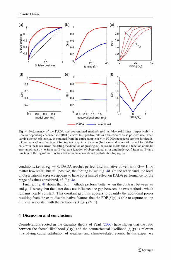
Fig. 4 Performance of the DADA and conventional methods (red vs. blue solid lines, respectively). aReceiver operating characteristic (ROC) curve: true positive rate as a function of false positive rate, whenvarying the cut-off level u, as obtained from the entire sample of n = 50 000 sequences; see text for details.b Gini index G as a function of forcing intensity λ1. c Same as (b) for several values of σQ and for DADAonly, with the black arrow indicating the direction of growing σQ. (d) Same as (b) but as a function of modelerror amplitude σQ. e Same as (b) but as a function of observational error amplitude σR . f Same as (b) as afunction of the logarithmic contrast between the conventional probabilities log p1/p0

conditions, i.e. as σQ → 0, DADA reaches perfect discriminative power, with G→ 1, nomatter how small, but still positive, the forcing is; see Fig. 4d. On the other hand, the levelof observational error σR appears to have but a limited effect on DADA performance for therange of values considered, cf. Fig. 4e.

Finally, Fig. 4f shows that both methods perform better when the contrast between p0and p1 is strong, but the latter does not influence the gap between the two methods, whichremains nearly constant. This constant gap thus appears to quantify the additional powerresulting from the extra discriminative features that the PDF f (y) is able to capture on topof those associated with the probability P(φ(y) ≥ u).

4 Discussion and conclusions

Considerations rooted in the causality theory of Pearl (2000) have shown that the ratiobetween the factual likelihood f1(y) and the counterfactual likelihood f0(y) is relevantin studying causal attribution of weather- and climate-related events. In this paper, we

Climatic Change

described data assimilation (DA) methods and demonstrated that they are well suited forderiving f0(y) and f1(y) from trajectories in the factual and the counterfactual worlds,respectively. Besides, these methods offer the key practical advantage of being alreadyup-and-running in real time at meteorological centers.

Combining these two sets of considerations, theoretical and practical, opens a novelroute towards real time, systematic causal attribution of weather- and climate-related events,thereby addressing a key challenge in the field of PEA at present (Stott et al. 2013).

4.1 Theoretical considerations

Implementing the DADA approach in the context of the L63 model in Section 3 allowedfor a detailed step-by-step illustration of our methodological proposal. It also provided abasic test for an initial performance assessment, which showed an improved level of dis-criminating power with respect to the conventional approach outlined in Section 1. Theseresults are promising, and their promise is easy to understand, given the fact that the DADAapproach leverages the available information on the entire trajectory y, as opposed to thesingle specific feature φ(y) ≥ u in the conventional approach.

It is important, though, to stress that the term “performance” here should be consideredwith caution: improving discriminatory performance may or may not be a desirable out-come, depending on the causal question being asked. Hannart et al. (2015) and Otto et al.(2015) have shown that the causal question being formulated reflects the subjective interestsof a particular class of end-users, and that the formulation itself may dramatically affect theanswer.

For example, the question “did anthropogenic CO2 emissions cause the heatwaveobserved over Argentina during January 2014?” has been traditionally treated by defininga “heatwave” in terms of a predefined temperature index reaching a predefined threshold,i.e., by a singular index exceeding a singular threshold. This class of questions matters forinstance in the context of insurance disbursements, where a financial compensation maytypically be triggered based on such an index exceedance. In this situation, the additionaldiscriminatory power of DADA is meaningless because the DADA computation does notaddress the question at stake: there is simply no alternative to computing the probabilitiesp0 and p1 of the index exceeding the threshold.

However, if the question is formulated instead as “did anthropogenic CO2 emissionscause the atmospheric conditions observed over Argentina during January 2014?” —i.e., without specifying which feature of the observed sequence is most important —then improving discrimination makes perfect sense and DADA becomes fully relevant.Furthermore, DADA is still fully relevant even if the question is formulated more specif-ically as “did anthropogenic CO2 emissions cause the damages generated in Argentinaby the atmospheric conditions of January 2014?,” provided that a model relating atmo-spheric observations to damages at every time step t along the trajectory of the physicalmodel used in the assimilation is available and can be integrated into the observationoperator H.

On the other hand, the results of Section 3 should also be considered with caution sim-ply because the L63 testbed obviously differs in many respects from the real situationenvisioned for future applications, both in terms of model dimension n and observa-tion dimension d: in practice n will be very large and d n, while here we tookd = n = 3.

Climatic Change

In particular, choosing a highly idealized, climatological prior distribution on the initialcondition π(x0) does not raise any difficulty under the tested conditions nor does it influencesignificantly the outcome of the procedure (not shown). The choice of π(x0), however,may be an important problem in practice, when d n, and lead to potentially spuriousresults.

As a consequence, it may be both necessary and useful to further constrain the so-calledbackground PDF π(x0) by using the forecasts originating from τ previous assimilationcycles, thus following the ideas of lagged-averaged forecasting (Hoffman and Kalnay 1983;Dalcher et al. 1988). The evidence thus obtained, though, will then also depend on previousobservations over the “initialization” window [−τ, ...,−1] — i.e., it will no longer repre-sent exclusively the desired evidence f (y). Besides, choosing τ optimally to constrain theinitial background PDF in a satisfactory manner, while at the same time limiting the latterunwanted dependence on previous observations, is a challenging question that needs to beadressed.

More generally, the problem of evaluating the evidence f (y) is not new in the HMM andDA literature; see, for instance, Baum et al. (1970); Hurzeler and Kunsch (2001); Pitt (2002)and Kantas et al. (2009). Various algorithms are thus available to carry out this evaluation,depending on a number of key assumptions — such as lack of Gaussianity or linearity —and on the inferential setting chosen, e.g. particle filtering. These algorithms may provideaccurate and effective solutions to the above problem, as well as improved alternatives to theGaussian and linear approximation of Eq. 5, since the latter may not be sufficiently accuratefor succesfully implementing the DADA approach under realistic conditions.

4.2 Practical considerations

While we have shown here that the proposal of using DADA for event attributions has intel-lectual merit, its main strength lies, in our view, in down-to-earth cost considerations. Bydesign, the DADA approach allows one to piggyback at a low marginal cost on the large andpowerful infrastructures already in place at several meteorological centers, in terms of bothhardware and personnel. These centers are capable of processing massive amounts of obser-vational data with high-throughput pipelines on the world’s largestcomputational platforms,as opposed to requiring the design, set-up and maintenance of a new and large, PEA-specificinfrastructure to collect observations and generate — under real time constraints — themany model simulations required by the conventional approach recalled in Section 1.

Taking a step back, it is useful to examine our proposal within the wider context of theemergence of so-called climate services. It is widely recognized that extending the scopeof activity of meteorological centers from being “monoline” weather forecasting providersto becoming “multiline” climate services providers – encompassing, for instance, weatherforecasting and weather event attribution as two service lines among several others –?? is arelevant strategic option (Hewitt et al. 2012). Such a strategy may foster the timely and cost-efficient emergence of the latter services by building upon technological and infrastructuresynergies with the former. For these reasons, our proposal is particularly relevant for, andcould contribute to, the implementation of the strategic option just outlined.

This being said, DADA can very well serve as a method for real time event attributioneven for hypothetical climate services providers that focus uniquely or mainly on longertime scales, beyond a month, a season or a year. In such a context, DADA may allow for theassimilation of a broader range of observations, and in particular of ocean observations; it

Climatic Change

may, in fact, be important to include the latter in causal analysis when the event occurrenceunder scrutiny is defined over a sufficiently large time window.

Finally, it is important to remember that providing real-time attribution assessments isa major communication challenge, since different methods give different answers and dif-ferent definitions of a specific event may also impact the outcome of an assessment — asmentioned above and as discussed recently by Trenberth et al. (2015). Various recent exam-ples, such as the ongoing California drought have shown that divergences among expertsmay lead to confusion in the media and among stakeholders. In this respect, a detailed com-parison of the DADA approach with other methods in realistic, real-time situations will berequired before the method can be applied operationally.

Appendix A: Illustration of the computational benefit of the DADAapproach

To illustrate the computational benefit, let Y be for instance a d-variate autoregressive pro-cess defined by Yt+1 = AYt + wt , where wt is an i.i.d. noise having known PDF g(·)and where A has the usual properties that insure stationarity (Gardiner 2004). We thenhave:

f (y) =T∏

t=1

g(yt − Ayt−1)π(y0) , (7a)

P(φ(Y) ≥ u) =∫

φ(y)≥u

T∏

t=1

g(yt − Ayt−1)π(y0)dy1,0 . . . dyd,0 . . . dyd,T , (7b)

with π(·) the prior PDF on the initial state Y0. Equation 7a shows that f (y) can be easilycomputed using a closed-form expression, while P(φ(Y) ≥ u) in Eq. 7b is an inte-gral on d × T + 1 dimensions which must instead be evaluated by using, for instance, acomputationally quite costly Monte-Carlo (MC) simulation.

Appendix B: Data Assimilation

The state-estimation problem for the system given by Eq. 4a and 4b has an exact solutiongiven by the following sequential Kalman filter (KF) equations:

xat = xf

t + K(yt − Hxft ) , (8a)

Pat = (I − KH)Pf

t , (8b)

xf

t+1 = Mxat , (8c)

Pf

t+1 = MPatM

′ + Q . (8d)

where ′ denotes the transpose operation. Here Eq. 8a and 8b are referred to as the analysisstep and denoted by a superscript a, while the forecast step is given by Eq. 8c and 8d, and isdenoted by a superscript f (Ide et al. 1997). The vector xa

t and the matrix Pat are the mean

and covariance of Xt conditional on (Y1, ...,Yt ) = (y1, ..., yt ); K = PftH

′(HPftH

′+R)−1 isthe so-called Kalman gain matrix; while Q and R are the covariances associated with vt and

Climatic Change

wt , respectively. Following (Wiener 1949), one distinguishes between filtering, in whichxat and Pa

t are conditioned only on the previous and current observations (y0,..., yt ), andsmoothing, in which they are conditioned on the entire sequence, 0 ≤ t ≤ T . Furthermore,the sequential algorithm needs to be initialized at time t = 0 with xf

0 and Pf

0 , which thusrepresent the a priori mean and covariance of X0, respectively, and have to be prescribed bythe user.

Appendix C: Derivation of the model evidence

In this appendix, we outline the derivation of model evidence within a general Bayesianframework, and we apply the latter to the narrower KF context to obtain Eq. 5. Con-sider two consecutive cycles of a DA run, the first with state vector xt and observationvector yt at instant t and the subsequent one with state vector xt+1 and observation vec-tor yt+1 at instant t + 1. We plan to find a tractable expression for the model evidencep(yt , yt+1).

The model evidence provided by the full sequence of observations y = (y0, ..., yT )

will be inferred by recursion, using the results of this two-observation setting. In order todecouple the two cycles, one first has to spell out the Bayesian inference p(yt , yt+1) =p(yt )p(yt+1|yt ). We look for a tractable expression for p(yt+1|yt ) by further introducingthe states xt+1 and xt as intermediate random variables:

p(yt+1|yt ) = ∫xt+1

p(yt+1|yt , xt+1)p(xt+1|yt ) dxt+1

= ∫xt+1

p(yt+1|xt+1){∫

xtp(xt+1|xt ) p(xt |yt ) dxt

}dxt+1 ,

(9)

where p(yt+1|xt+1) is the likelihood of the observation vector yt+1 conditional on the statevector xt+1 and it is known from Eq. 4b. The conditional PDF p(xt |yt ) of xt on yt at instantt — which appears on the right-hand side of the above equation — is referred to as theanalysis PDF in the DA literature, where it is denoted by a superscript a (Ide et al. 1997),and it constitutes the main DA output. The integral

∫xt

p(xt+1|xt )p(xt |yt ) dxt = p(xt+1|yt ),in which p(xt+1|xt ) is known from the model dynamics given by Eq. 4, propagates thisanalysis PDF further in time, to instant t + 1. Hence, the result of this integration coincideswith the forecast PDF, denoted by superscript f in the DA literature (Ide et al. 1997). Itfollows that this decomposition is tractable using a DA scheme that is able to estimate theconditional and forecast PDFs.

Next, let us apply the general Bayesian inference (9) to the case in which all the PDFsinvolved are Gaussian; this requires, in turn, that both the dynamics and observation modelsM and H be linear, and that the input statistics all be Gaussian. In this case, the Kalmanfilter allows for the exact computation of the PDFs mentioned in Eq. 9, which turn out to beGaussian.

In the following, N (x,P) designates the Gaussian PDF of mean x and covariance matrixP. In this context, the analysis PDF at instant t is N (xa

t ,Pat ), where xa

t and Pat are the anal-

ysis state and error covariance matrix at instant t . As a result of the linearity assumptions,the forecast PDF at instant t + 1 is given by a Gaussian distribution N (xf

t+1,Pf

t+1), where

xf

t+1 and Pf

t+1 are the forecast state and error covariance matrix at instant t + 1. Further, theintegration on xt+1 in Eq. 9 can readily be performed under these circumstances, with theoutcome that p(yt+1|yt ) is distributed as N (Hxf

t+1,R + HPf

t+1 H′).

Climatic Change

The desired model evidence f (y) can then be computed by recursion on successive timesteps as:

f (y) = p(y0)

T∏

t=1

(2π)−d2 |�t |− 1

2 exp

{−1

2(yt − Hxf

t )′�−1t (yt − Hxf

t )

}; (10)

here p(y0) represents the prior PDF of the initial state, �t = R + HPft H

′, and this expres-sion coincides with Eq. 5 and can be evaluated with the help of any DA method that yieldsthe forecast states and forecast error covariance matrices, such as the KF or the EnKF. Notethat the traditional standard Kalman smoother would give the same result as the KF, sincethey share the same forecasts.

Finally, Eqs. 9 and 10 above show that the likelihood f (y) may be obtained as a by-product of the inference on the state vector x, which usually is the main purpose in numericalweather prediction. This idea may actually be highlighted in even greater generality byconsidering the equality:

f (y) = p(y|x)p(x)p(x|y) . (11)

While Eq. 11 is a direct consequence of Bayes theorem, it also illustrates a point that isarguably not so intuitive. The likelihood f (y) is obtained here as the ratio of two quantities:a numerator p(y|x)p(x) that is a model premise inherently postulated by Eq. 4a and 4b, anda denominator p(x|y) that may be viewed as the end result of the primary inferxence onx. In other words, estimating f (y) requires only a straightforward division, provided x hasbeen previously inferred.

Equation 11 thus expresses with great clarity and simplicity a fundamental idea but-tressing our proposal, as it provides a general theoretical justification for the suggestion ofderiving the likelihood from an inferential treatment that focuses on x. To put it succintly,this equation basically says, “He who can do more can do less.” In the context of DA, whoseend purpose is to infer the state vector x out of an observation y — i.e., the more part — itis possible to obtain the likelihood as a by-product thereof — i.e., the less part — and thusalmost for free.

Appendix D: PDF of the state vector

We associate a label ω ∈ � with each realization of the random process vt that drivethe model given by Eq. 6. The PDF of the state vector xt can be obtained as the numer-ical solution of the corresponding Fokker-Planck equation, and it is the mean over � ofthe sample measures obtained for each realization ω of the noise vt and (Chekroun et al.2011, and references therein). Each sample measure is supported on a random attractorthat may have very fine structure and be time-dependent (Chekroun et al. 2011, Figs. 1–3 and supplementary material), but the PDF is supported smoothly, in the counterfactualworld in which λ0 = 0, on a “thickened” version of the fairly well-known strange attrac-tor of the original L63 model. The latter PDF represents its attractor in dynamic system’sterminology.

Acknowledgements It is a pleasure to thank Fredi Otto and Daithı Stone, who provided careful and con-structive reviews of the original paper. This work has been supported by grant DADA from the AgenceNationale de la Recherche (ANR, France: AH and all co-authors) and by the Multi-University ResearchInitiative (MURI) N00014-12-1-0911 from the the U.S. Office of Naval Research (MG).

Climatic Change

References

Allen MR (2003) Liability for climate change. Nature 421:891–892Baum LE, Petrie T, Soules G, Weiss N (1970) A maximization technique occurring in the statistical analysis

of probabilistic functions of Markov chains. Ann Math Stat 41(1):164–171Balmaseda MA, Alves OJ, Arribas A, Awaji T, Behringer DW, Ferry N, Fujii Y, Lee T, Rienecker M, Rosati

T, Stammer D (2009) Ocean initialization for seasonal forecasts. Oceanography Special Issue 22(3)Bengtsson L, Ghil M, Kallen E (1981) Dynamic meteorology: Data assimilation methods. Springer-Verlag,

New YorkBhend J, Franke J, Folini D, Wild M, Bronnimann S (2012) An ensemble-based approach to climate

reconstructions. Clim Past 8:963–976Bocquet M, Pires CA, Wu L (2010) Beyond Gaussian statistical modeling in geophysical data assimilation.

Mon Wea Rev 138:2997–3023Bocquet M (2012) Parameter-field estimation for atmospheric dispersion: application to the Chernobyl

accident using 4D-Var. Quart J Roy Meteor Soc 138:664–681Bucklew JA (2004) Introduction to rare event simulation. SpringerCarrassi A, Vannitsem S (2010) Model error and variational data assimilation: A deterministic formulation.

Mon Wea Rev 138:3369–3386Carrassi A, Ghil M, Trevisan A, Uboldi F (2008) Data assimilation as a nonlinear dynamical systems

problem: Stability and convergence of the prediction-assimilation system. Chaos: An InterdisciplinaryJournal of Nonlinear Science 18(2):023–112

Chekroun MD, Simonnet E, Ghil M (2011) Stochastic climate dynamics: Random attractors and time-dependent invariant measures. Phys D 240(21):1685–1700. doi:10.1016/j.physd.2011.06.005

Chevallier F (2013) On the parallelization of atmospheric inversions of CO2 surface fluxes within avariational framework. Geosci Model Dev Discuss 6:37–57

Christidis N, Stott PA, Scaife AA, Arribas A, Jones GS, Copsey D, Knight JR, Tennant WJ (2013) A NewHadGEM3-A-Based System for Attribution of Weather- and Climate-Related Extreme Events. J Clim26(9):2756–2783

Cosme E, Brankart JM, Verron J, Brasseur P, Krysta M (2006) Implementation of a reduced-rank, square-rootsmoother for ocean data assimilation. Ocean Model 33:87–100

Dalcher A, Kalnay E, Hoffman RN (1988) Medium-range lagged average forecasts. Mon Wea Rev 116:402–416. doi:10.1175/1520-0493. 1988116¡0402:MRLAF¿2.0.CO;2.

Del Moral P, Garnier J (2005) Genealogical particle analysis of rare events. Ann Appl Probab 15(4):2496–2534

Evensen G (2003) The ensemble Kalman filter: theoretical formulation and practical implementation. OceanDyn 53:343–367

Gardiner C (2004) Handbook of stochastic methods for physics, Chemistry and the natural sciences.Publisher. Pls.; no web tonite

Gelb A (1974) Applied optimal estimation. M.I.T. Press, CambridgeGhil M, Childress S (1987) Topics in geophysical fluid dynamics: Atmospheric dynamics, dynamo theory

and climate dynamics. Springer-Verlag, New York, p 485Ghil M, Malanotte-Rizzoli P (1991) Data assimilation in meteorology and oceanography. Adv Geophys

33:141–266Ghil M, Cohn S, Tavantzis J, Bube K, Isaacson E (1981). In: Bengtsson L, Ghil M, Kallen E (eds) Applica-

tions of estimation theory to numerical weather prediction. In: Dynamic meteorology: Data assimilationmethods. Springer Verlag, pp 139–224

Gini C (1921) Measurement of inequality of incomes. Econ J 31(121):124–126. doi:10.2307/2223319Greenland S, Rothman KJ (1998) Measures of effect and measures of association, Chapter 4. In: Rothman

KJ, Greenland S (eds) Modern Epidemiology, 2nd edn.,Lippincott-Raven, Philadelphia, USAHannart A, Pearl J, Otto FEL, Naveau P, Ghil M (2015) Counterfactual causality theory for the attribution of

weather and climate-related events. Bull Am Meteorol Soc. in pressHarris TE, Kahn H (1951) Estimation of particle transmission by random sampling. Natl Bur Stand Appl

Math Ser 12:27–30Heidelberg P (1995) Fast simulation of rare events in queueing and reliability models. ACM Trans Models

Comput Simul 5:43–85Hewitt C, Mason S, Walland D (2012) The global framework for climate services. Nat Clim Change 2:831–

832Hoffman RN, Kalnay E (1983) Lagged average forecasting, an alternative to Monte Carlo forecasting. Tellus

35A:100–118. doi:10.1111/j.1600-0870.1983.tb00189.x

Climatic Change

Houtekamer PL, Mitchell HL, Pellerin G, Buehner M, Charron M (2005) Atmospheric data assimilation withan ensemble Kalman filter: Results with real observations. Mon Wea Rev 133:604–620

Hurzeler M, Kunsch HR (2001). In: Doucet A, De Freitas JFG, Gordon NJ (eds) Approximation and max-imising the likelihood for a general state-space model. In: Sequential Monte Carlo Methods Practice.Springer-Verlag, New York

Ide K, Courtier P, Ghil M, Lorenc A (1997) Unified notation for data assimilation: Operational, sequentialand variational. J Meteor Soc Japan 75:181–189

Ihler AT, Kirshner S, Ghil M, Robertson AW, Smyth P (2007) Graphical models for statistical inference anddata assimilation. Phys D 230:72–87

Jazwinski AH (1970) Stochastic and filtering theory. Mathematics in sciences and engineering series 64:376

Kalman RE (1960) A new approach to linear filtering and prediction problems. J Basic Eng 82D:33–45

Kantas N, Doucet A, Singh SS, Maciejowski JM (2009) An overview of sequential Monte Carlo methods forparameter estimation. In: General state-space models, IFAC System Identification, no. Ml

Kondrashov D, Sun CJ, Ghil M (2008) Data assimilation for a coupled ocean-atmosphere model. Part II:Parameter estimation. Mon Wea Rev 136:5062–5076. doi:10.1175/2008MWR2544.1

Kondrashov D, Shprits Y, Ghil M (2011) Log-normal Kalman filter for assimilating phase-space density datain the radiation belts. Space Weather 9:S11006. doi:10.1029/2011SW000726

Lee TCK, Zwiers FW, Tsao M (2008) Evaluation of proxy-based millennial reconstruction methods. ClimateDyn 31:263–281

Lorenz EN (1963) Deterministic non-periodic flow. J Atmos Sci 20:130–141Lorenz MO (1905) Methods of measuring the concentration of wealth. Publications of the American

Statistical Association 9(70):209–219. doi:10.2307/2276207Martin MJ et al. (2014) Status and future of data assimilation in operational oceanography. J of Oper Ocean.

in pressMassey N, Jones R, Otto FEL, Aina T, Wilson S, Murphy JM, Hassell D, Yamazaki YH, Allen MR

(2014) weather@home — development and validation of a very large ensemble modelling system forprobabilistic event attribution. Q J R Meteorol Soc. doi:10.1002/qj.2455

Otto FEL, Boyd E, Jones RG, Cornforth RJ, James R, Parker HR, Allen MR (2015) Attribution of extremeweather events in Africa: a preliminary exploration of the science and policy implications. ClimaticChange

Palmer TN (1999) A non-linear dynamical perspective on climate prediction. J Clim 12:575–591Pearl J (2000) Causality: Models, reasoning and inference. Cambridge University Press, CambridgePitt MK (2002) Smooth particle filters for likelihood evaluation and maximisation. Warwick Economic

Research Papers, No. 651Robert C, Blayo E, Verron J (2006) Comparison of reduced-order sequential, variational and hybrid data

assimilation methods in the context of a Tropical Pacific ocean model. Ocean Dyn 56:624–633Roques L, Chekroun MD, Cristofol M, Soubeyrand S, Ghil M (2014) Parameter estimation for energy

balance models with memory. Proc R Soc A 470:20140349Ruiz J, Pulido M, Miyoshi T (2013) Estimating model parameters with ensemble-based data assimilation: A

review. JMSJ 91(2):79–99Sakov P, Counillon F, Bertino L, Lister KA, Oke PR, Korablev A (2012) TOPAZ4: an ocean-sea ice data

assimilation system for the North Atlantic and Arctic. Ocean Sci 8:633–656. doi:10.5194/os-8-633-2012Stone DA, Allen MR (2005) The end-to-end attribution problem: from emissions to impacts. Clim Change

71:303–318Stott PA et al. (2013). In: Asrar GR, Hurrell JW (eds) Attribution of weather and climate-related events, in:

Climate Science for Serving Society: Research, Modelling and Prediction Priorities. Springer. in pressStott PA, Stone DA, Allen MR (2004) Human contribution to the European heatwave of 2003. Nature

432:610–614Talagrand O (1997) Assimilation of observations, an introduction. J Meteor Soc Japan 75(1B):191–209Tandeo P, Pulido M, Lott F (2014) Offline parameter estimation using EnKF and maximum likelihood error

covariance estimates: Application to a subgrid-scale orography parametrization. Q J R Meteorol Soc.doi:10.1002/qj.2357

Trenberth KE, Fasullo JT, Shepherd TG (2015) Attribution of climate extreme events. Nature Clim Change5:725–730

Wiener N (1949) Extrapolation, Interpolation and smoothing of stationary time series, with engineeringapplications. M.I.T. Press, Cambridge, p 163

Wouters J, Bouchet F (2015) Rare event simulation of the chaotic Lorenz 96 dynamical system. GeophysicalResearch Abstracts, EGU General Assembly 2015 Vol. 17, EGU2015-10421-1