DA10.6: Implementation of the PLM Process model for the ... · CMMS Computerised Maintenance...
67
Copyright © PROMISE Consortium 2004-2008 DELIVERABLE NO DA10.6: Implementation of the PLM Process model for the Demonstrator DISSEMINATION LEVEL CONFIDENTIAL DATE 15.05.2008 WORK PACKAGE NO WP A10: Bombardier VERSION NO. V.2.1 ELECTRONIC FILE CODE DA10 6 v2.1_FINAL_23_05_2008.doc.1 CONTRACT NO 507100 PROMISE A Project of the 6th Framework Programme Information Society Technologies (IST) ABSTRACT This deliverable (DA10.6) summarises the implementation of the PLM process model for the demonstrator, in terms of scenes, PROMISE components and technology implemented, as described in DA10.3 and DA10.4. The motivation for eventual discrepancies is given, together with the detailed results of the activities performed for the implementation. STATUS OF DELIVERABLE ACTION BY DATE (dd.mm.yyyy) SUBMITTED (author(s)) Jong-Ho SHIN 11.04.2008 VU (WP Leader) Marcel Huser 15.05.2008 APPROVED (QIM) Kiritsis Dimitris 23.05.2008 Written by: Jong-Ho SHIN, Ralf Heckmann, Bertram Winkenbach,Gerd Grosse, Altuğ Metin DA10.6: Implementation of the PLM Process model for the Demonstrator
Transcript of DA10.6: Implementation of the PLM Process model for the ... · CMMS Computerised Maintenance...

Copyright © PROMISE Consortium 2004-2008
DELIVERABLE NO DA10.6: Implementation of the PLM Process model for the
Demonstrator
DISSEMINATION LEVEL CONFIDENTIAL
DATE 15.05.2008
WORK PACKAGE NO WP A10: Bombardier
VERSION NO. V.2.1
ELECTRONIC FILE CODE DA10 6 v2.1_FINAL_23_05_2008.doc.1
CONTRACT NO 507100 PROMISE A Project of the 6th Framework Programme Information Society Technologies (IST)
ABSTRACT This deliverable (DA10.6) summarises the implementation of the PLM process model for the demonstrator, in terms of scenes, PROMISE components and technology implemented, as described in DA10.3 and DA10.4. The motivation for eventual discrepancies is given, together with the detailed results of the activities performed for the implementation.
STATUS OF DELIVERABLE
ACTION BY DATE (dd.mm.yyyy)
SUBMITTED (author(s)) Jong-Ho SHIN 11.04.2008
VU (WP Leader) Marcel Huser 15.05.2008
APPROVED (QIM) Kiritsis Dimitris 23.05.2008
Written by: Jong-Ho SHIN, Ralf Heckmann, Bertram Winkenbach,Gerd Grosse, Altuğ Metin
DA10.6: Implementation of the PLM Process model for the Demonstrator

Copyright © PROMISE Consortium 2004-2008 Page ii
@
Revision History
Date (dd.mm.yyyy)
Version Author Comments
13.03.2008 0.1 Jong-Ho SHIN DRAFT
28.03.2008 0.2 Jong-Ho SHIN DRAFT
11.04.2008 0.3 Jong-Ho SHIN DRAFT
Author(s)’ contact information Name Organisation E-mail Tel Fax Jong-Ho SHIN EPFL [email protected] 0041 21 693 73 31 0041 21 693 35 09 Ralf HECKMANN Bombardier
Transportation [email protected]
+49 271 702 708 +49 271 702 346
Bertram WINKENBACH Bombardier Transportation
+49 7249 387139 +49 7249 387139
Altuğ Metin InMediasp [email protected] +49 3302 559 431

Copyright © PROMISE Consortium 2004-2008 Page 3
@
Table of Contents 1 INTRODUCTION................................................................................................................................6
1.1 PURPOSE OF THIS DELIVERABLE ....................................................................................................6 1.2 OBJECTIVE OF DEMONSTRATOR.....................................................................................................6
2 DESCRIPTION OF THE DEMONSTRATORS ..............................................................................7 2.1 FIELD DATA...................................................................................................................................7
2.1.1 Definition of field data.............................................................................................................7 2.1.2 Sources and processing of field data .......................................................................................9 2.1.3 Structure and link between field data ....................................................................................22 2.1.4 Data provisioning and restrictions in A10.............................................................................24
2.2 APPLICATION SCENARIOS AND EMBEDDING INTO THE ENGINEERING DESIGN PROCESS................25 2.3 SELECTION OF COMPONENT.........................................................................................................28
2.3.1 Boundary conditions for selecting components .....................................................................28 2.3.2 Selected components for A10.................................................................................................29
2.4 MODIFICATION TO INITIAL PROMISE APPROACH.......................................................................31 2.4.1 BT DSS module modification.................................................................................................31
3 ANALYSIS OF RESULTS OBTAINED IN THE ACTIVITIES A10.6........................................34 3.1 FIELD DATA TRANSFER FROM BT DATABASE TO PDKM .............................................................34
3.1.1 Diagnosis Data Structure ......................................................................................................34 3.1.2 Data integration architecture ................................................................................................37
3.2 DATA ACCESS TO PDKM ............................................................................................................39 3.3 DEVELOPMENT AND TEST OF THE STAND-ALONE DSS ................................................................40 3.4 GUI DEVELOPMENT ......................................................................................................................1
4 CONCLUSION ....................................................................................................................................2
5 REFERENCES.....................................................................................................................................3 List of figures FIGURE 1. FLOW OF FIELD DATA .....................................................................................................................8 FIGURE 2. BASIC MAXIMO IT- STRUCTURE ................................................................................................10 FIGURE 3. OVERVIEW ON MAXIMO VEHICLE STRUCTURE..............................................................................11 FIGURE 4. OVERVIEW ON MAXIMO DATA AQUISITION AND PROCESSING.................................................12 FIGURE 5. STRUCTURE OF C&C SYSTEM FOR TRAXX LOCOMOTIVE BR185.................................................14 FIGURE 6. FAULT DETECTION, STORAGE AND OUTPUT ON VEHICLE................................................................15 FIGURE 7. TRANSFER OF DIAGNOSTICS DATA FROM VEHICLE TO GSM-MANAGER (CDDB) ..........................18 FIGURE 8. EVALUATION OF DIAGNOSTIC DATA WITH WINDIA AND CENTRAL DIAGNOSTICS DATABASE
(CDDB)................................................................................................................................................18 FIGURE 9. DIAGNOSTICS EVALUATION TOOL WINDIA...................................................................................19 FIGURE 10. ENVIRONMENTAL DATA MASK SUBSYSTEM DCPU ....................................................................20 FIGURE 11. ENVIRONMENTAL DATA MASK SUBSYSTEM ZSG .......................................................................20 FIGURE 12. ENVIRONMENTAL DATA MASK SUBSYSTEM ASG.......................................................................21 FIGURE 13. ENVIRONMENTAL DATA MASK SUBSYSTEM BSG .......................................................................22 FIGURE 14. STRUCTURE OF A FAM (MAXIMO) ...........................................................................................23 FIGURE 15. TABLESTRUCTURE OF CONFIGURATIONDATA INSIDE CDDB........................................................24 FIGURE 16. FRACAS PROCESS ......................................................................................................................26 FIGURE 17. DATA COVERAGE OF COMPONENTS.............................................................................................29 FIGURE 18. WORKFLOW DIAGRAM FOR P6 .....................................................................................................32 FIGURE 19. LEVEL 2: INFORMATION FLOW DIAGRAM FOR P6 .........................................................................33 FIGURE 20: DIAGNOSIS DATABASE ................................................................................................................35

Copyright © PROMISE Consortium 2004-2008 Page 4
@
FIGURE 21: VEHICLE DATABASE....................................................................................................................36 FIGURE 22: CONFIGURATION DATABASE .......................................................................................................37 FIGURE 23: DATA INTEGRATION ARCHITECTURE............................................................................................38 FIGURE 24: BT ENVIRONMENTAL DATA.........................................................................................................39 FIGURE 20. PROMISE DSS ARCHITECTURE ..................................................................................................40 FIGURE 21. BT DSS USER SCENARIO..............................................................................................................42 FIGURE 22. COEFFICIENT OF ENVIRONMENTAL OPERATING DATA TO FAILURE CODE EVENT RATE .................52 FIGURE 23. GRAPH FOR SINGLE CLUSTERING RESULT.....................................................................................54 FIGURE 24. DIFFERENT TYPE OF GRAPH FOR SINGLE CLUSTERING RESULT .....................................................55 FIGURE 25. GRAPH FOR MULTI CLUSTERING RESULT......................................................................................56 List of Tables TABLE 1. RAM(S) INFORMATION PROVIDED BY FRACAS PROCESS .............................................................13 TABLE 2. DESCRIPTION OF FIGURE 18 DIAGRAM ............................................................................................32 TABLE 3. DESCRIPTION OF FIGURE 2DIAGRAM...............................................................................................34 TABLE 4. ‘DINF FOR FAILURE CODE’ RESULT ................................................................................................46 TABLE 5. COMPARISON BETWEEN ‘DINF FOR FAILURE CODE’ AND ‘DINF FOR FAILURE EVENT’ ..................49 TABLE 6. COEFFICIENT CALCULATION RESULT...............................................................................................51 TABLE 7. SINGLE CLUSTERING RESULT...........................................................................................................53 TABLE 8. MULTI CLUSTERING RESULT ...........................................................................................................57 Abbreviations Abbreviations used in this document: BOL Beginning of life BT Bombardier Transportation CBM Condition Based Maintenance CM Condition Monitoring CMMS Computerised Maintenance Management System DCPU Display and Control Processing Unit DfX Design for X DSS Decision Support System EBoK Engineering Book of Knowledge (e.g. DfRAM/LCC-, DfS- or DfE-EBoK) ECC ERP Central Component EDP Engineering Design Process FAM Failure report stored in the FRACAS database FPMK Failures Per Million Kilometer FRACAS Failure Reporting Analysis and Corrective Action System GDU Gate Drive Unit GUI Graphical User Interface HD Hard Disk (to transfer FAM and Diagnostics Data to A10 partners) HVIM High Voltage Industrial Modules ID Ident (-number) IGBT Insulated Gate Bipolar Transistor IOCI Inter-Organisational Communication Infrastructure LCC Life Cycle Cost MCB Main Circuit Breaker MDBF Mean Distance Between Failure MOL Middle of life RAM Reliability, Availability & Maintainability PDKM Product Data & Knowledge Management PDM Product Data Management

Copyright © PROMISE Consortium 2004-2008 Page 5
@
PEID Product Embedded Information Device RAMS Reliability, Availability, Maintainability, Safety TCMS Train Control and Management System TRAXX Bombardier Locomotive Platform Name UML Unified modelling language WBS work breakdown structure

Copyright © PROMISE Consortium 2004-2008 Page 6
@
1 Introduction
1.1 Purpose of this deliverable
The ‘Implementation of the PLM Process model for the Demonstrator’ describes how the PLM process is applied into the BT DSS demonstrator. Hence, the objective of this document is to check the implemented PLM process for the DfX in Bombardier application and the related PLM components necessary for the implementation of PLM process compared to the previously designed PLM process and PLM components in DA10.3 and DA10.4. For this purpose, the necessary comoponents for BT DSS demonstrator are described in the following section 2. In the next section 3, the implemented BT DSS module is explained based on the user scenario in this document. To show the effectiveness of BT DSS module, a sample test and its result are explained in the same section. In addition, a new version of BT DSS GUI is added in appendix to help understaning of BT DSS module.
1.2 Objective of demonstrator The objective of BT DSS is to close the loop of information from the experience embedded in field data to the knowledge needed by engineers to improve the design so that it could produce more competitive products. To do this, BT DSS focuses on the transformation of field data into DSS knowledge. From the objective of BT DSS, BT DSS will provide
• information on reliability indices based on failure code event rate of the considered systems;
• information on root causes of failures and faults of the considered systems; the possible causes should be ranked on their resp. likelihood
• information on the clustering of field data/diagnosis data/environmental operating data of TRAXX locomotive
For the BT DSS module, the evaluation method of failure code event rate and the root cause analysis method are adapted. The data mining method is also included so as to provide DfX specialist engineer with an overview of environmental operating data status and their relationship. Product/Projects in focus: If not stated otherwise in the component specific chapters the product/projects considered shall be the TRAXX locomotive family with focus on loco types BR185.1 and its components/parts.

Copyright © PROMISE Consortium 2004-2008 Page 7
@
DSS input: In principal, all data input for the DSS come from four sources:
1. Data of corrective and preventive actions applied to the vehicle. 2. Failure report of locmotive 3. Locomotive diagnostics data: errors 4. Locomotive diagnostics data: environmental operating data
DSS output
1. The evaluated rank of the event rate of failure code 2. The relationship between failure code event and environmental operating data 3. The clustering of environmental operating data
The output shall be provided as diagrams, tables, listings or text files, whatever is appropriate for the desired purpose.
2 Description of the demonstrators
2.1 Field data
2.1.1 Definition of field data During the design phase of a technical system (BOL) the most important input, beside new information obtained by research, is experience. It enables you to reuse available knowledge, reduces development time and effort and helps to avoid errors (old and new ones). To a wide extend experience is directly gained by practical daily engineering work and stored in the heads of the engineers. With increasing complexity of technical systems, the need to document experience in a way that allows its processing with means of modern IT techniques became essential. One of the most important parameter in this regard are field data. Field data in our context are all data describing the reliability, availabilty, maintainability and safety behavoiur of a considered system during commissioning, operation and decommissioning. If applicable, life cycle cost parameters may be included. All parameters have to be defined in a unique and retraceable way. Field data could be gathered by a formal failure-reporting process (FRACAS) or by means of an automated technical monitoring systems. In case of the DSS both ways are used to provide information. In principal, all data input for the DSS come from these sources:

Copyright © PROMISE Consortium 2004-2008 Page 8
@
1. FRACAS data: data of corrective and preventive actions applied to the vehicle. 2. Locomotive diagnostics data:
incidents 3. Locomotive diagnostics data:
environmental operating data
Figure 1. Flow Of Field Data
It is important to distinguish between the data gained by FRACAS process and the data gained by the diagnostics system. A failure recorded by the FRACAS process is always related with a physical exchange of a component of the locomotive. The failure rate is the probability of a malfunction (failure) per unit time at time t for any member of the original population (of components), n(0). It is a direct indicator of the system’s reliability.

Copyright © PROMISE Consortium 2004-2008 Page 9
@
An incident recorded by the diagnostics system is not necessarily linked with the failure and exchange of a component. It could just indicate a defined operating condition or a deviance from that. The time behaviour of the incidents related to a parameter like the FCODE (type of incident) or a vehicle ID number we shall call incident rate. With every incident a snapshot of specific environmental data is taken.
2.1.2 Sources and processing of field data As mentioned in chap. 2.1.1 all provided field data to be used in the DSS come from three sources, which are explicated in more detail in the following chapters.
1a. Data of corrective actions applied to the vehicle after the occurrence of a failure or the detection of a fault. These so called FRACAS data are held by the BT MAXIMO database. A failure/fault report is called FAM. The selected FAM reports for this project are given in [6].
1b. For the consideration of the component ‘wheel’ data it was planned to use data provided by the RM/ENOTRAC data base VipsCarsis containing data of preventive maintenance and overhaul activities in addition to the data 1a .
Due to a change in the Promise A10 workgroup these data could not be made available to be used for the DSS.
2. Locomotive diagnostics data: incident (error) file. These event driven data are stored onboard the locomotive and are transmitted via GSM to the BT diagnostics database (defined headers see [9]).
There are nearly 6.000 predefined error codes and associated information [8] which are the most important link to the FRACAS database [6].
3. Locomotive diagnostics data: operating environment data. These data are updated in the locomotive per second.
Every event causing an incident/error code triggers a snapshot of selected operating environment data. For every system monitored by the diagnostic system a data set of operating environment data (freeze frame) is predefined (see examples chap. 2.1.2.2.6). An overview of all covered indicators (about 1.500) is given in[7].
2.1.2.1 FRACAS The central data administration within FRACAS is run by Maximo (MRO Software Ltd./Boston), a computerized maintenance management tool.

Copyright © PROMISE Consortium 2004-2008 Page 10
@
It is based on a relational database using Windows technology and has the capability to communicate via the internet. BT has Maximo integrated into its data management system BTRAM where the interfaces to other databases are provided (i.e. commercial data via SAP for spare part provisioning or other application modules like the use of handheld for data aquisition).
Figure 2. Basic Maximo IT- Structure
Out of these general infrastructure (BTRAM) only the Maximo core competences are relevant for further considerations. Maximo covers all RAM relevant field data of every component of a locomotive down to the smallest exchangeable unit (LRU) triggered by a failure event or a part exchange activity. In addition to the part monitoring for each vehicle its individual structure is also registered and monitored (so every phase of a vehicle modification is retraceable). This structure is an ‘as-built’ structure, not a functional structure, because the field data are always related to a physical component. The component will take its data with it if it is transferred to another vehicle or into a stock. Figure 3 gives an overview on the principles of such an ‘as-built’ vehicle structure as it is laid down in Maximo.

Copyright © PROMISE Consortium 2004-2008 Page 11
@
Figure 3. Overview on Maximo Vehicle Structure
To evalute the reliability behaviour of the locomotives monthly reports are compiled out of Maximo. These reports rely on the FRACAS data (FAM). Except the usage of the vehicle’s mileage to calculate the time dependend failure rate, there is no link to the diagnostics data. A full link to the diagnostics system will be established first time by using the DSS/DfX technique. The number of data sets accumulated in time by Maximo is very little compared to the data gathered in time by the diagnostics system. Therefore it is sufficient for the time being to have a Maximo data provisioning on demand to the DSS/DfX (about once per week). In principle an automated interface based on Oracle between the Maximo server and the diagnostics system is technically feasible but not needed at all costs. Figure 4 gives an overview on the structure of information which is gained out of the field data gathered with Maximo (beside its task as part of the maintenance management process).

Copyright © PROMISE Consortium 2004-2008 Page 12
@
Figure 4. Overview on Maximo Data Aquisition and Processing Table 1 shows the RAM(S) information which can be made available by the data of the FRACAS process. Therefore this information need not to be generated redundantly bei the DSS/DfX process. The essential progress of the DSS/DfX is the connection of this information with the information inclosed in the diagnostics data to create a new level of information.

Copyright © PROMISE Consortium 2004-2008 Page 13
@
Table 1. RAM(S) Information provided by FRACAS Process
Configuration Management
• (Vehicle Asset Management) • Asset History Tracking • Condition Monitoring • Modification Status Tracking • Warranty Status management Product Introduction • Configuration Management • Fault/defect reporting • (Work order management) • Change management (Mod. Orders) • (Inventory Management) • (Labour & Material Management) • (Warranty Management) • Mileage Recording & tracking • Maintain equipment history Warranty Management • Component Warranty Tracking • Customer & Supplier Warranty Status • Correlation of defects by supplier • Liability attribution • Component defects & failure history Maintenance Management • (Maintenance Planning) • Fault/defect reporting • (Work order management) • (Configuration Management) • (Inventory Management) • (Labour & Material Management) • (Activity recording) • Mileage Recording & tracking • Maintain Equipment history Feedback/Reporting • Contract performance • Vehicle performance • Component performance

Copyright © PROMISE Consortium 2004-2008 Page 14
@
Diagnostics data The TRAXX locomotive is equipped with Bombardiers diagnostics system DAVIS185. The system gathers and stores diagnostic information from all different subsystems on the vehicle. The acquisition of this diagnostic information is event driven, based on failure detection of components and logging of operational states on the vehicle.
Figure 5. Structure of C&C system for TRAXX locomotive BR185
Part of every diagnostics data set is a collection of additional information about the “environmental condition” at the time when the event happens. This environment data contains a timestamp, a GPS position and a snapshot of individual defined process data (environment data mask). This environment data is gathered and stored exactly at this time when the event happens and gives the user of the diagnostics system additional information about process data on the vehicle (e.g. catenary voltage and current, traction force, battery power, …). For a standard TRAXX locomotive approximately 6000 different codes are defined in a diagnostics data model (see extract in file “ERROR_CODES.PDF”). Parts of this model are definitions for:

Copyright © PROMISE Consortium 2004-2008 Page 15
@
• Failure codes which where triggered if a component fails. • Protocol codes, which will be triggered to log operational states of the vehicle,
e.g. “Main switch on/off”, “drivers desk occupied”, “vehicle speed exceeds 3km/h”, … .
From a technical point of view, both types of events are handled inside the diagnostic system in the same way and use the same software routines. The data which is stored in the diagnostic system on the vehicle is provided to the users in three different ways:
• Visualization on the onboard displays for the train driver. • Download of diagnostics memory with a local service access and evaluation of
the vehicle data with a tool on the service computer. • Remote data transfer of the diagnostic memory to a database server and
evaluation of the data with a tool which is able to access directly the database server.
The diagnostic system DAVIS185 installed on each TRAXX locomotive includes the following components and functionalities:
Figure 6. Fault detection, storage and output on vehicle

Copyright © PROMISE Consortium 2004-2008 Page 16
@
Onboard on vehicle: • Data acquisition in subsystem (subsystem diagnostics functionality), the status of
each failure code is represented in the subsystem as a binary signal with the two states 0 (= no fault) and 1 (= fault).
• Data transfer of a complete diagnostic data set (DDS) from subsystem into non volatile memory (NFS) of central diagnostics system.
• Non volatile memory (NFS) where all diagnostic events are stored for visualization purposes (operational and maintenance diagnostics).
Offline at groundstation:
• Remote data transfer of diagnostics events from vehicle to groundstation with GSM-Manager.
• Storage of diagnostic events offline in central diagnostics database (CDDB) which is part of GSM-Manager.
• Data evaluation with toolset which can be linked to data in diagnostic database (CDDB).
2.1.2.1.1 Data acquisition in subsystem (fault detection) The data acquisition in the subsystems (like ZSG, ASG, DCPU, …) of the vehicle is implemented as a one time check during startup of the subsystem to detect self test errors and a cyclic check of failure indicators to detect malfunctions of components during operation. If one of these indicators notifies a malfunction of a component a diagnostic event is generated and sent to the central diagnostics system. Each individual diagnostic event that represents the malfunction of a component is identified by a unique failurecode. The detection of malfunctions of a component is implemented as a software routine. These routines are part of the vehicle control software. The output of this routines are diagnostic data sets (DDS) which can be sent over to central diagnostics system via a standard communication link (MVB, CAN, Ethernet, …) inside the vehicle.
2.1.2.1.2 Data transfer from subsystem into central diagnostics system A complete diagnostics data set (DDS) is transferred from the subsystem to the central diagnostics system and stored in the non volatile memory (NFS). The DDS contains the following data:
• error code, • timestamp t0, • geographical position at t0 (based on GPS data), • environment data mask (a snapshot of process data at t0) with additional vehicle
mileage.
2.1.2.1.3 Storage of event data in non volatile memory (fault storage and output)
Copyright © PROMISE Consortium 2004-2008 Page 17
@
The non volatile storage of the event data on the vehicle is used to collect all the diagnostics events transferred from the subsystems. The event data is stored in the onboard database and provides the information which is visualized on the onboard displays. There are different display masks available to visualize the event data for the two target groups train driver and maintenance personal.
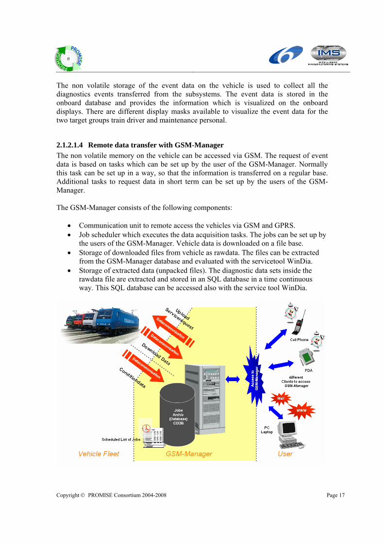
2.1.2.1.4 Remote data transfer with GSM-Manager The non volatile memory on the vehicle can be accessed via GSM. The request of event data is based on tasks which can be set up by the user of the GSM-Manager. Normally this task can be set up in a way, so that the information is transferred on a regular base. Additional tasks to request data in short term can be set up by the users of the GSM-Manager. The GSM-Manager consists of the following components:
• Communication unit to remote access the vehicles via GSM and GPRS. • Job scheduler which executes the data acquisition tasks. The jobs can be set up by
the users of the GSM-Manager. Vehicle data is downloaded on a file base. • Storage of downloaded files from vehicle as rawdata. The files can be extracted
from the GSM-Manager database and evaluated with the servicetool WinDia. • Storage of extracted data (unpacked files). The diagnostic data sets inside the
rawdata file are extracted and stored in an SQL database in a time continuous way. This SQL database can be accessed also with the service tool WinDia.

Copyright © PROMISE Consortium 2004-2008 Page 18
@
Figure 7. Transfer of diagnostics data from vehicle to GSM-Manager (CDDB)
2.1.2.1.5 Storage of diagnostics events in central diagnostics database All event data which is downloaded via GSM from the vehicles is stored in the central diagnostics database (CDDB). The CDDB is a standard SQL database which is configured to be used to store event data for a complete vehicle fleet. This database can be accessed by an appropriate toolset which is provided by Bombardier.
Figure 8. Evaluation of diagnostic data with WinDia and Central Diagnostics
Database (CDDB)
2.1.2.1.6 Data evaluation with toolset linked to diagnostics data in CDDB To access the diagnostics data stored in the central diagnostics database an appropriate toolset is available. The evaluation can be based on single vehicles up to complete vehicle fleets. Access to the diagnostic data stored in the SQL database (CDDB) is not based on different files. This format is only used to download data from the vehicle. This file can be also directly evaluated with WinDia.

Copyright © PROMISE Consortium 2004-2008 Page 19
@
To visualize diagnostic data offline the service tool WinDia is used. WinDia provides a chronological view on the diagnostic data sets for the whole vehicle fleet. In addition a statistical view based on pivot tables is available to provide a quick overview of the fault status for a complete vehicle fleet.
Figure 9. Diagnostics Evaluation Tool WinDia
For each subsystem a different set of environment data is linked to the fault codes. This data set is defined as a mask and optimized to give a view on the condition of the vehicle and special process data inside the subsystem. These data sets are used to do an extended evaluation inside the Promise project. The following screenshots shows the content of the different masks linked to the different subsystems: DCPU

Copyright © PROMISE Consortium 2004-2008 Page 20
@
Figure 10. Environmental Data Mask Subsystem DCPU
ZSG
Figure 11. Environmental Data Mask Subsystem ZSG
ASG

Copyright © PROMISE Consortium 2004-2008 Page 21
@
Figure 12. Environmental Data Mask Subsystem ASG
BSG

Copyright © PROMISE Consortium 2004-2008 Page 22
@
Figure 13. Environmental Data Mask Subsystem BSG GSM-Manager server and SQL database CDDB is located inside the intranet of Bombardier. Access from outside to this server is without permission of Bombardier not possible. Data access for the Promise project is established by duplicating the SQL database CDDB to a harddisk and hand over the complete harddisk to the team members. The SQL database is running under a Microsoft SQL-Server with Windows Server 2003 as operating system. The access to this SQL database is performed exclusively by WinDia. The software interface to access the CDDB is based on stored procedures. A direct access via SQL commands is also possible. The connection to the database can be established by a standard database interface (like ODBS or JDBC).
2.1.3 Structure and link between field data
2.1.3.1 FRACAS (Maximo) Below it is pointed out, how the field data dealing with components failures are structured and how the link between these Maximo data and the diagnostics data is established. Figure 14 gives the structure of a FAM. The data fields (HEADER) in combination with the information about the vehicle structure (including all quantities of parts in a fleet etc.) contain all information to calculate the RAM(S) behaviour of the considered locomotive (beside the figures for the mileage, see chap. 2.1.2). To get evidence about a potential root cause of a failure we need information which may be stored in (very many) related diagnostics data sets. The link between a FAM and the concerned diagnostic data (incident data file) is given by the error code and/or the error description associated with it [8]. This data field (Diagnostic Code or FCODE) is marked red in the figure below. Not in every FAM a figure for this FCODE is available (almost none mechanical component has one). In case of a missing FCODE in a FAM, you may find the related incident file by the date, the name of the failed system/component or other common data fields (marked red in Figure 14, also see [9] and [10]). The link between the incident file and the related environmental operating data is given by the structure and relations of the provided SQL database defined in [10].

Copyright © PROMISE Consortium 2004-2008 Page 23
@
To understand the way of data storage and coding within the diagnostics data base, you have follow the instructions in [10].
Figure 14. Structure of a FAM (Maximo)
2.1.3.2 Diagnostic data Diagnostics information which is stored in CDDB is divided in two major datasets. Each dataset contains several tables:
• (Compressed) rawdata which is downloaded from the vehicle and stored in CDDB.
• Configuration data which is defined and provided by the engineering of the vehicle during the design. Configuration data is updated on the CDDB by the database administrator.
Rawdata downloaded from vehicle and stored into CDDB contains all information about the faults that happens on the vehicle over a period of time. It contains data like:
• fault code, • timestamp, • geographical position (based on GPS data), • Environment data, compressed in a dataframe • … .

Copyright © PROMISE Consortium 2004-2008 Page 24
@
To interpret the data in a correct way the configuration data is necessary. Configuration data provides the instruction how to:
• link a text message to the error code, • unpack environment data (scaling of values, units, datatype and byteoffset in
dataframe, …). Configuration data can vary over different software releases. Thus it is necessary to use the correct set of configuration data related to the software release which is actually installed on the vehicle. For the interpretation of the different datatypes inside a diagnostics data set the configuration data is splitted into several tables: Error! Objects cannot be created from editing field codes.
Figure 15. Tablestructure of configurationdata inside CDDB
2.1.4 Data provisioning and restrictions in A10 The data containing the information according to chap. 2.1.2 article 1a, 2 and 3 have been provided by Bombardier Transportation stored on a hard disk (HD) to the Promise A10 partners. As mentioned in chap. 2.1.2 the data according to article 1b could not be made available to WP A10. This had an significant influence on the selection of the component to be considered (see chap. 2.3). The HD transferred to the project partners holds about 1.530 FAM of a selected fleet of locomotives and components and about 105 million sets of diagnostics data, containing about 4,2 billion individual data fields. Due to the complex process of decoding the evironmental data and the great amount of data to manage, solving the task of data provisioning, data linkage and calculating during the DSS realisation, caused considerable difficulties. In addition, a certain effort of manual data pre-processing was unavoidable (data cleaning process etc.) Therefore a limit of about 2 million data sets for developing and testing the DSS was agreed by the A10 working team. The consequences on the data input result mainly in a restriction of the number of the considered vehicles/components (to get less FAM) and a restriction of the time span in which to search for related diagnostics data sets. The consequences of these restrictions on the results of the Promise A10 WP are a limitations on the practical technical significance of the outcome and limited answers on

Copyright © PROMISE Consortium 2004-2008 Page 25
@
questions of algorithm performance etc. . But it does not restrict conclusions on the principal applicability of the choosen DSS/DfX process. It is to mention that these data and the detailed documentation concerning the data structure [10] are strictly confidential and subject to [11]. All information stored on the transferrred HD remain property of Bombardier Transportation and is only to be used within the PROMISE project to test and evaluate the choosen processes and tools. It shall not be published in any way. The publishing of the results of the evaluation is also subject to the rules agreed on in [11].
2.2 Application scenarios and embedding into the engineering design process
We consider the EDP in the BOL phase of a railway vehicle, a system or component. In this project phase the basic hard- and software requirements of the regarded system are defined (technical specification). As shown in the picture below, this process is widely influenced by experience gained in the operational use of the considered system resp. their antecedents with comparable functions.

Copyright © PROMISE Consortium 2004-2008 Page 26
@
Figure 16. FRACAS Process
Beside the technical information given by specifications, suppliers, standards etc. the main pool of knowledge is comprised in gathered field data and diagnostics data. While field data focus on quality indicators (like reliability, availability, maintenance efforts, etc.) diagnostics data contain information about the operational environment and the behavior of parameters in the context of failures and faults. The combinations of these two sources of information can create new knowledge which gives the engineer strong hints on i.e. failure causes, systematic errors and other information necessary to enhance the quality of a newly designed systems. Up to now, this combination of data is not only a wasteful task. In many cases the knowledge is hidden behind complex dependencies and therefore never discovered. It is the task of the DSS/DfX to support the process of the - design of new technical systems - redesign of existing systems due to changed external requirements (feasibility) - redesign of existing systems due to unmet requirements (root cause analysis)

Copyright © PROMISE Consortium 2004-2008 Page 27
@
With a DSS/DfX process implemented, the engineer shall be provided with a single point of entry to all these available information (raw data) in convenient graphical way, as outlined in the GUI in chap. 3.4. This feature is important, because not every information contained in the raw data will be subject to the algorithm in any case. Therefore the engineer shall have the possibility to get access to the full data information after he gets a design hint following the scenarios described below. This should be able in a most structured, convenient and self-evident way. The quality of the implemented GUI is most important for the acceptance of the tool and the entire process by the user. Besides the raw data access, the focus of the DfX is to consider all available information and extract knowledge out of it. The flow of data is given in Figure 1. The data integrated into the DSS/DfX implementation are marked red. To achieve the extraction of knowledge in a most efficient way, the DSS/DfX demonstrator provides approaches for different scenarios of BOL engineering. 1st Scenario: The new system to be designed is based on a functional antecedent. If the system worked well there is no need to make extensive changes (forget about commercial aspects etc.). If there were specific problems in the past, the engineer will know about it. So he should be able to choose specific parameters to the DfX on which the investigation (algorithm) is based. The result will give specific information (by using all available information from field data and diagnostics data) to support the engineer finding the related failure causes, inadequate operational conditions, etc. (i.e. specific answer to a specific problem). 2nd Scenario: The new system to be designed is based on a functional antecedent. The system didn’t perform very well due to random failures/faults. In this case the engineer has no specific hints which parameter cause the trouble and what to be searched for. The DfX tool/process now will provide methods to cluster the data by suitable algorithms (i.e. data mining, pattern search) as shown in chap. 3. The result will enable the engineer to find weak points in the design, architecture, component behavior or in the operational environment (root cause analysis). The result of the 2nd scenario could be used for specific investigations as shown in the 1st scenario.

Copyright © PROMISE Consortium 2004-2008 Page 28
@
3rd Scenario: The new system to be designed is based on a functional antecedent. The system performed well, but faces enhanced requirements (by law, customer, market situation, etc.). In this case the engineer has to check the influence of the changed conditions on specific indicators of the system (i.e. reliability). This can be done by sorting and filtering data of system behaviour gathered under similar conditions as given by the new enhanced conditions. With the sound knowledge of the influence of measured (field-)parameters on specific system parameters (i.e. failure rate), the engineer is in a position to find feasable solutions (economical, reliable, safe, ...). Because these dependencies are unknown at first, the engineer will start with 2nd scenario. The result of the 2nd scenario could be used for specific investigations as shown in the 1st scenario. Example: Using (diagnostics-)data of locomotive operating in summer and winter time, the influence of the temperature to a specific failure rate (FRACAS data) could be estimated. Knowing this, a decision if an invention or improvement of the air conditioning system will pay off could be made.
2.3 Selection of component
2.3.1 Boundary conditions for selecting components The availability of data depends on the kind of component. Field data: Safety related, non redundand components (like wheels) shall never fail randomly (because this could cause severe accidents). Therefore no data for corrective maintenance (= failures) are available. To achive this, these components underlay a very rigid preventive maintenace shedule. These kind of data will therefore provided in the test data set. Electronical components underlay almost no preventive activities. They fail randomly. So for these components failure data (FAM) can be provided. Some components are in between, like the MCB. They comprise an electrical part and a mechanical part. The four choosen test components are selected to cover the entire range of practical possibilities. Diagnostics data: The availabilty of diagnostics data depends on the connectivity of the considered component to the onboard control system.

Copyright © PROMISE Consortium 2004-2008 Page 29
@
Components of the control system itself have a very good coverage. Mechanical components are not extensively monitored in terms of diagnostics (they are maintained preventively). This will for sure change in future and the DfX process will support this development by its gained knowledge. The picture below gives a survey of the data coverage of the choosen components:
Figure 17. Data Coverage of Components
2.3.2 Selected components for A10 The considered components for A10 - Wheel - Main Circuit Breaker - Gate Drive Unit - DCPU Board Type BHPC1 are described in detail in [1]. Therefore only the finally selected component ‘DCPU Board Type BHPC1’ (see chap. 2.4) is specified below. DCPU Board Type BHPC1 Component in focus: CPU board BHPC1 within DCPU device

Copyright © PROMISE Consortium 2004-2008 Page 30
@
Brief description of the BHPC1 function: The BHPC1 device contains the CPU for the DCPU. It’s a complete computer board based on a Pentium II and was developed as the control computer for the display devices on TRAXX locomotives. The device has two Ethernet and one MVB ports as communication interface. The CPU is located in a closed aluminium case to fulfill EMC/ESD and climate requirements. The operating system and the application software is stored on a IDE-Compact-Flash-Disk. Technical data/requirements: Mass: 2100 Gramm Power supply: (back-plane-utility-plug) : +3.3V, +5V, +12V Power consumption: ca. 20 Watt CPU: Pentium II / 266 MHz Interfaces: 1x PS2-keyboard 1x PS2-mouse 2x RS232 ports 1x 4 COM-port to BHIO-board 1x MVB port 2x Ethernet port Temperature: -25°C to +75°C (in operation) -40°C bis +85°C (non operating) Manufactured in accordance to: Shock and vibration EN 50155:1995 Climate and environment EN 50155:1995 EMC/ ESD tested on ENV 50121-3-2 (CE-Conformity) Temperature- and voltage monitoring: Two temperature measuring devices are integrated into the BHPC1-board. They are monitored via the internal SMB-Bus. The system voltage is controlled by a supervisorchip LM80 kontrolliert and monitored via SMB-Bus (High-Signal means voltage is within specific boundaries): IN0 : V-CPUPU (+2.5V) IN2 : +3.3V IN4 : +12V IN6 : not connected IN1 : VTT (+1.8V) IN3 : +5V IN5 : not connected Product/Projects in focus: TRAXX AC2 through BR185.1, BR185.2, 146.1, BR146.2, Re482.1, Re482.2 and others.

Copyright © PROMISE Consortium 2004-2008 Page 31
@
2.4 Modification to initial PROMISE approach As explained in chap. 2.1.4 the amount of processable data was restricted due to the effort of data provisioning, preprocessing and handling. These conditions led to the decision, to consider only one single type of component out of the selection given in [1] and to choose the component with the highest ratio of diagnostics data to FAM. As shown in Figure 17 this component is the DCPU Board Type BHPC1. For this component definitely faced no problem of data availability. During the working period of WP A10 the requirements to the DSS and the implementation of the underlaying algorithm passed several stages. In the beginning there was a straight forward approach of evaluating failure data to create reliability indicators mirrored against Pareto’s law. It became evident very soon that this approach will not necessarily lead to an improvement of the existing analysis techniques (like reliability reporting tools), because the huge reservoir of information buried in the diagnostics data would still left untouched. The consequent idea was to combine the failure data with the related environment and operating data of the diagnostics data and open the possibilities of root cause analysis and similar aspects. Focussing on diagnostics data and using the failure data as focal point drove the decision to choose the BHPC1 as reference component. It it obvious that under these aspects the unavailability of the field data of the component ‘wheel’ was not a big loss to WP A10, because with this component there are no diagnostics data existing, at all.
2.4.1 BT DSS module modification According to the new user requirement of BT DSS, BT DSS module is modified. The BT DSS module is modified to provide more improved information and knowledge that is related to reliability of failure code event. First of all, the evaluation of failure code event is performed based on the failure code event rate. The result of evaluation is used by DfX specialist engineers in discriminate critical failure codes. In addition, the modified BT DSS module adapts data mining technique for the intuitive understanding of field data/diagnosis data/environmental operating data of TRAXX locomotive. Hence, the clustering method is included in the modified BT DSS module. The modified BT DSS module is described as modified work flow diagram in the Figure 18. Table 2 describes work flow model depicted in Figure 18.

Copyright © PROMISE Consortium 2004-2008 Page 32
@
Level1_E7
P2
E2
E5
E3
E6
E4
Level 1_P6
P3
P5
P6
Level1_E8
P4
P1
E1
E7
P7
Figure 18. Workflow diagram for P6
Table 2. Description of Figure 18 diagram Modelling components Description Remarks
P1 Select failure report (FAM) P2 Set parameters for DSS module P3 Calculate DINF of failure codes P4 Select critical failure codes P5 Calculate coefficient between failure code
and field data
P6 Start clustering for single field data
Process
P7 Start clustering for failure event Level1_E7 Data ranges with changed information
content available in DSS together wit analysis criteria
E1 Failure reports are selected E2 Entering parameters values is finished
Event
E3 DINF of failure code is calculated

Copyright © PROMISE Consortium 2004-2008 Page 33
@
E4 failure codes are selected E5 Coefficient is calculated E6 Single clustering is finished E7 Multiple clustering is finished Level1_E8 DfX knowledge generated
Condition (at branching and merging)
According to the modification of workflow diagram of P6, information flow of P6 is also changed. The modified information flow and its description are explained in the Figure 19 and Table 3.
Figure 19. Level 2: Information flow diagram for P6

Copyright © PROMISE Consortium 2004-2008 Page 34
@
Table 3. Description of Figure 19 diagram Modelling components Description Remarks
P1 Select failure report (FAM) P2 Set parameters for DSS module P3 Calculate DINF of failure codes P4 Select critical failure codes P5 Calculate coefficient between
failure code and field data
P6 Start clustering for single field data
Process
P7 Start clustering for failure event Level1_I7 Data transferred into DSS I1 FAM list from PDKM I2 Selected failure report (FAM) list I3 Entered parameter values for DSS I4 Failure records from PDKM I5 DINF calculation result I6 Selected critical failure codes I7 Field data I8 Calculated coefficient I9 Single clustering result I10 Multi clustering result
Information
Level1_I8 DfX knowledge
3 Analysis of results obtained in the Activities A10.6
3.1 Field data transfer from BT database to PDKM
3.1.1 Diagnosis Data Structure Field data that is relevant for PROMISE analyses will be gathered systematically and in a company database. This database contains field data from different sources:
• data from service PCs • data from GSM manager • online submitted data via GPRS or WLAN
The main characteristic of the submitted data is that a record set contains a snapshot of the onboard systems with selected measurement values. This snapshot will be created everytime a failure is detected by the integrated diognosis system. According to the type of the failure appropriate system parameters will be attached to the record set. The data will be stored in an encoded format using different masks. The mask that is applied

Copyright © PROMISE Consortium 2004-2008 Page 35
@
depends on several parameters such as vehicle configuration, database version, platform id and year. Figure 20 gives an overview to the diagnosis database:
Figure 20: Diagnosis Database
Furthermore information about all vehicles are stored in a vehicle database. This database helps to establish the semantical connection between gathered data and the configuration structure of diagnosis data (Figure 21).

Copyright © PROMISE Consortium 2004-2008 Page 36
@
Figure 21: Vehicle Database
The configuration of the diagnosis data structure is included in the configuration database (Figure 22). This database covers information about the data masks and is mainly required in order to decode the stored values in the diognosis database. Furthermore textual informaiton regarding possible failures and measurement values are also stored in this database.

Copyright © PROMISE Consortium 2004-2008 Page 37
@
Figure 22: Configuration Database
3.1.2 Data integration architecture The diagnosis data for the years 2001-2006 has been provided as a MS SQL database. In order to make this data available within the PDKM system an integration architecture has been developed. The architecture includes a data interpreter for BT diagnosis data which is capable of analysing the database and extracting field data that can be represented within the PDKM system. The extracted data will be transformed to a PMI compatible format so that every system that implements this interface can easily handle this data. In the case of the application scenario A10, field data is uploaded into the PDKM system using the PMI interface.

Copyright © PROMISE Consortium 2004-2008 Page 38
@
Once the data is available within the PDKM system DSS algorithms can access this data and perform calculations. The database integration between these systems enables the identification and retrieval of relevant data for A10. The results of DSS calculations will be presented to the user via the DSS GUIs in the PDKM/DSS portal.
MS SQL SERVER
BT Diagnosis Database
A10 Data Interpreter(T-SQL Procedure)
HTTP/SOAP Endpoint
PDKM/DSS (SAP BOMBARDIER)
SAP ECC Database
DSS Algorithms
PDKM/DSS Portal GUIs
PMI Interface
Figure 23: Data integration architecture
In the PDKM database a record set is represented by a Notification object (Figure 24) Unlike in the concepts for other PROISE application scenarios, the object pair measuring point/measurement document was not used in A10. The reason for this divergency is that there are many field data values captured simultaneously („snapshot of system values“) and stored as a record set. This mechanism is best reflected by a Notification object which covers additional data for BT Environmental data. Each information item is identified by an object ID. The same amount of environmental data will also be represented in the PDKM portal.

Copyright © PROMISE Consortium 2004-2008 Page 39
@
Figure 24: BT Environmental data
3.2 Data access to PDKM The connection between the DSS and the PDKM is depicted in the next figure. It shows an overview of the architectural concepts upon which PROMISE decision support system deployments are based. A more detailed look on the DSS-architecture is provided in DR8.8 “Implementation of PROMISE DSS prototype version 3”.
Copyright © PROMISE Consortium 2004-2008 Page 40
@
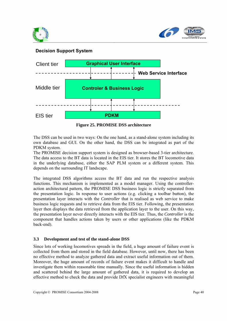
Decision Support System
Controler & Business Logic
PDKMEIS tier
Graphical User InterfaceClient tier
Middle tier
Web Service Interface
Figure 25. PROMISE DSS architecture
The DSS can be used in two ways: On the one hand, as a stand-alone system including its own database and GUI. On the other hand, the DSS can be integrated as part of the PDKM system. The PROMISE decision support system is designed as browser-based 3-tier architecture. The data access to the BT data is located in the EIS tier. It stores the BT locomotive data in the underlying database, either the SAP PLM system or a different system. This depends on the surrounding IT landscape. The integrated DSS algorithms access the BT data and run the respective analysis functions. This mechanism is implemented as a model manager. Using the controller-action architectural pattern, the PROMISE DSS business logic is strictly separated from the presentation logic. In response to user actions (e.g. clicking a toolbar button), the presentation layer interacts with the Controller that is realised as web service to make business logic requests and to retrieve data from the EIS tier. Following, the presentation layer then displays the data retrieved from the application layer to the user. On this way, the presentation layer never directly interacts with the EIS tier. Thus, the Controller is the component that handles actions taken by users or other applications (like the PDKM back-end).
3.3 Development and test of the stand-alone DSS
Since lots of working locomotives spreads in the field, a huge amount of failure event is collected from them and stored in the field database. However, until now, there has been no effective method to analyze gathered data and extract useful information out of them. Moreover, the huge amount of records of failure event makes it difficult to handle and investigate them within reasonable time manually. Since the useful information is hidden and scattered behind the large amount of gathered data, it is required to develop an effective method to check the data and provide DfX specialist engineers with meaningful

Copyright © PROMISE Consortium 2004-2008 Page 41
@
knowledge transformed from the raw data. For this objective, BT DSS provides the evaluation method for the change of failure code event rate and the correlation method between failure code event rate and environmental operating data. Also, BT DSS provides a data clustering method so as to show field data as an intuitive way. Hence, BT DSS is useful for DfX specialist engineers to understand field data as a congested form of information about failure code event rate in the viewpoint of reliability. To do this, BT DSS has three main sub modules: (1) DINF calculation for the evaluation of the change of failure code event rate and DINF calculation for each failure code event, (2) multi linear regression module to correlate DINF of failure code event with environmental operating data, and (3) clustering module to group environmental operating data having similar values. DINF is a kind of index which represents the status of the change of failure code event event occurrence over time. To calculate DINF, we define the failure code event rate of each failure code as the measure for the DINF calculation. The failure code event rate of each failure code is calculated from the failure events in the PDKM database. Since the DINF of failure code shows the status of occurrence of failure code event, the DINF of each failure code can be compared and helps DfX specialist engineers to find critical failure codes and related components/parts since DfX specialist engineers would like to reduce focusing components/parts to be checked. From the result of the DINF of each failure code, DfX specialist engineers select critical failure codes which have high value of the DINF for failure code value which means that these failure codes have worse characteristics of the failure code event change during observation period. After the selection of critical failure codes, BT DSS calculate the criticality, abnormality, and severity at each failure code event for the selected failure code during observation period and the criticality, abnormality, and severity are aggregated into the DINF for failure event as the same way of the DINF of failure code. The DINF for failure event is a evaluation of each failure event whenever failure event happens for the same failure code. Combining the DINF for failure event and environmental operating data, BT DSS module builds a multi linear regression model and solves it to get the coefficient between environmental operating data and the DINF for failure event. The coefficient of environmental operating data explains the effect of environmental operating data on the change of the DINF for failure event. The more correlated environmental operating data has higher and lower value with the change of the DINF for failure event. Hence, it can help engineers to find the root cause of the change of DINF for failure event. After DfX specialist find suspicious environmental operating data from the multi linear regression model. At the next step, DfX specialist engineers can perform clustering method which groups environmental operating data having similar values. From the clustering of environmental operating data, DfX specialist engineers can recognize the environmental status. The following Figure 26 shows the user scenarion of BT DSS module.

Copyright © PROMISE Consortium 2004-2008 Page 42
@
3. Calculate DINF for
failure codeby DSS
2. Input parameter values
by DfX specialist engineer
4. Select failure code by DfX
specialist engineer
1. Select FAMby DfX specialist
engineer
5. Calculate DINF for
failure eventby DSS
Failure codeevent rate
Environmental operating data
DINF for failure code
DINF for failure event
Failure codeevent rate
6. Calculate coefficientby DSS
Coefficient
8. Make single clusteringby DSS
Clusters for each
environmental operating data
9. Make multiple
clusteringby DSS
Environmental operating data
Environmental operating data
Clusters for failure event
Output InputDSS scenario
7. Start clusteringby DfX specialist
engineer
Procedure by user
DSS result
Procedure by DSS
Database in PDKM
Data input by user
Scenario procedure
Output of procedure
Input of procedure
Select kind of analysis
Calculate clusters
Calculate DINF/coefficient
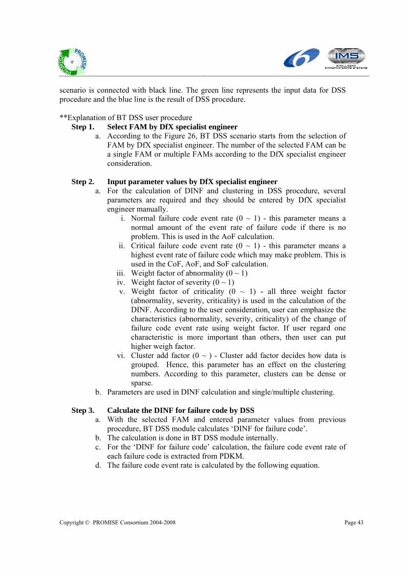
Figure 26. BT DSS user scenario
Figure 26 consists of three main parts. The left square box contains the result of DSS procedure following the scenario. The middle one shows BT DSS user scenario and the right one is the input data for the DSS procedure. The DSS procedure according to user
Copyright © PROMISE Consortium 2004-2008 Page 43
@
scenario is connected with black line. The green line represents the input data for DSS procedure and the blue line is the result of DSS procedure. **Explanation of BT DSS user procedure
Step 1. Select FAM by DfX specialist engineer a. According to the Figure 26, BT DSS scenario starts from the selection of
FAM by DfX specialist engineer. The number of the selected FAM can be a single FAM or multiple FAMs according to the DfX specialist engineer consideration.
Step 2. Input parameter values by DfX specialist engineer
a. For the calculation of DINF and clustering in DSS procedure, several parameters are required and they should be entered by DfX specialist engineer manually.
i. Normal failure code event rate (0 ~ 1) - this parameter means a normal amount of the event rate of failure code if there is no problem. This is used in the AoF calculation.
ii. Critical failure code event rate (0 ~ 1) - this parameter means a highest event rate of failure code which may make problem. This is used in the CoF, AoF, and SoF calculation.
iii. Weight factor of abnormality (0 ~ 1) iv. Weight factor of severity (0 ~ 1) v. Weight factor of criticality (0 ~ 1) - all three weight factor
(abnormality, severity, criticality) is used in the calculation of the DINF. According to the user consideration, user can emphasize the characteristics (abnormality, severity, criticality) of the change of failure code event rate using weight factor. If user regard one characteristic is more important than others, then user can put higher weigh factor.
vi. Cluster add factor (0 ~ ) - Cluster add factor decides how data is grouped. Hence, this parameter has an effect on the clustering numbers. According to this parameter, clusters can be dense or sparse.
b. Parameters are used in DINF calculation and single/multiple clustering.
Step 3. Calculate the DINF for failure code by DSS a. With the selected FAM and entered parameter values from previous
procedure, BT DSS module calculates ‘DINF for failure code’. b. The calculation is done in BT DSS module internally. c. For the ‘DINF for failure code’ calculation, the failure code event rate of
each failure code is extracted from PDKM. d. The failure code event rate is calculated by the following equation.

Copyright © PROMISE Consortium 2004-2008 Page 44
@
0
ijij
ij
nt t
λ =−
(1)
: failure code number, 1 4000: the index of failure code event for the same failure code , 1: failure code event rate of failure code at failure code event : cumulated occurrence number
thij
ij
i ij i j
i jnλ
≤ ≤≤
0
of failure code at failure code event : failure code event time of failure code at failure code event : initial time of observation
th
thij
i jt i jt
e. Then, using failure code event rate, criticality for fcode (CoF),
abnormality for fcode (AoF), and severity for fcode (SoF) are calculated. f. To calculate criticality for fcode (CoF), abnormality for fcode (AoF), and
severity for fcode (SoF), BT DSS uses following equations.
1( )
1 , , 0
n
ic ijj
i ic ij ic ijic
CoF if thenn
λ λλ λ λ λ
λ=
−= − < − =
×
∑ (2)
1
1
( ( )), ( ), ( )=0
( ( ))
n
ij ie ijj
i ij ie ij ij ien
ic ie ijj
tAoF if t then t
t
λ λλ λ λ λ
λ λ
=
=
−= ≤ −
−
∑
∑ (3)
( 1)
( 1) ( 1) ( 1)1
( 1) ( 1)
( 1)1
, 0, 0
nij i j
ij i j ij i j ij i jji n
ic ij i j ij i j
ij i jj
t tSoF if then
t t t tt t
λ λλ λ λ λ
λ
−
− − −=
− −
−=
−− − −
= < =− −
−
∑
∑ (4)
i i i iDINF for failure code CoF AoF SoFα β γ= × + × + × (5)
: failure code number, 1 4000: the index of failure code event, 0: failure code event rate of failure code at failure code event : critical failure code event rate of failure code (
thij
ic
ie
i ij j
i ji
t
λλλ
≤ ≤≤
0
) : normal failure code event rate of failure code at : failure code event time of failure code at failure code event : initial time of observation : weight factor for criticality: weigh
ij ij
thij
i tt i jtαβ t factor for abnormality
: weight factor for severityγ
Copyright © PROMISE Consortium 2004-2008 Page 45
@
g. Criticality for fcode (CoF) shows how much failure code event rate is close to the critical level of failure code event rate. For all failure code events of each failure code, the difference between critical level of failure code event rate and current failure code event rate ( ic ijλ λ− ) is summed and normalized by the worst case of failure code event rate ( icn λ× ). The worst case of failure code event rate ( icn λ× ) means that the failure code event rate always shows up to the critical level during observation period. The low value of criticality for fcode (CoF) means that less failure code event occurs so that it has been in good status.
h. Abnormality for fcode (AoF) shows how much failure code event rate is apart from the normal level of failure code event rate. For all failure code events of each failure code, the difference between normal level of failure code event rate and current failure code event rate ( ( )ij ie ijtλ λ− ) is summed and normalized by the worst case of abnormal status of failure code event rate ( ( )ic ie ijtλ λ− ). The worst case of abnormal status of failure code event rate ( ( )ic ie ijtλ λ− ) means that the failure code event rate always shows the maximum abnormal level as much as critical level of failure code event rate. The high value of abnormality for fcode (AoF) means that failure code event rate is far from normal status of failure code event rate so that it has been in bad status.
i. Severity for fcode (SoF) shows how quickly failure code event rate increase. For all failure events of each failure code, the slope between previous failure code event rate and current failure code event rate ( ( 1)
( 1)
ij i j
ij i jt tλ λ −
−
−−
) is summed and normalized by the worst case of failure code
event rate increase (( 1)
ic
ij i jt tλ
−−). The worst case of failure code event rate
increase (( 1)
ic
ij i jt tλ
−−) means that the failure code event rate always increases
up to maximum slope. The high value of severity for fcode (SoF) means that failure code event rate increases much so that it has been in bad status.
j. The DINF is a kind of index value which shows how defined measure changes during observation period. The DINF evaluates the change of defined measure over time so that it can be used as an indicator to show how defined measure is in good status. Hence, it is applicable to any measure that changes over time. For example, if we can define measure of performance of components/parts in locomotive, then we can discriminate components/parts having low performance compared to others by DINF calculation method. Currently, in Bombardier DSS, the DINF calculate and evaluate event rate change of failure code as measure in the view point of reliability of failure code. ‘DINF for failure code’ is a weighted sum of criticality for fcode (CoF), abnormality for fcode (AoF), and severity for fcode (AoF).
k. The result of this procedure is as follows.

Copyright © PROMISE Consortium 2004-2008 Page 46
@
Table 4. ‘DINF for failure code’ result
fcode criticality for fcode
abnormality for fcode
severity for fcode
DINF for failure code RANK
---- MA000334 FAM_reports ----- 3995 0.06016297 0.059974961 0.0024324 0.12257 14014 0.0498402 0.049790926 0.0022272 0.101858 23984 0.03865338 0.038461072 4.10E-04 0.077524 33985 0.03856593 0.038373606 4.09E-04 0.077348 44005 0.02873855 0.028544257 6.52E-04 0.057935 54006 0.02385323 0.023657966 7.04E-04 0.048215 64015 0.02287605 0.022680585 2.83E-04 0.045839 74003 0.01854868 0.018352349 3.35E-04 0.037236 84004 0.01419861 0.014001411 2.53E-04 0.028453 91633 0.00916812 0.00896991 0.0065168 0.024655 103993 0.00892422 0.008725962 2.53E-04 0.017903 114012 0.00892421 0.008725952 2.53E-04 0.017903 12
l. The objective of ‘DINF for failure code’ is to find focusing failure codes
among several failure codes which happen during observation period from FAM. From the rank of failure code, DfX specialist engineer can select failure codes which have worse characteristics of the change of failure code event rate during observation period. Criticality for fcode (CoF), abnormality for fcode (AoF), and severity for fcode (AoF) are the measuring values to show characteristics of the failure code event rate change over time.
m. The high value of ‘DINF for failure code’ means that the failure codes happen frequently and much, and increase abruptly. Hence, the high ranked failure code by the value of the DINF for failure code should be considered as critical failure code and checked the cause of failure code by DfX specialist engineer.
n. Criticality means how many failure code event happens, abnormality means how much failure code event rate is different from the normal failure code event rate, and severity means how quickly failure code event rate increases.
o. Criticality for fcode (CoF), abnormality for fcode (AoF), and severity for fcode (AoF) are a normalized value by the worst case of each characteristic (CoF, AoF, and SoF). Hence, they have a normalized value from zero to one respectively. The value ‘one’ means that the failure code event rate shows worst case of criticality, abnormality, or severity during whole observation period. For example, criticality for fcode (CoF) of 3995 in DINF calculation is 0.06016297 in Table 4. This means that the failure code event rate shows about 6% criticality compared to the worst case of criticality. The worst case of criticality is defined as the failure code event rate always reaches as much as up to the critical level during whole

Copyright © PROMISE Consortium 2004-2008 Page 47
@
observation period. Abnormality for fcode (AoF) and severity for fcode (SoF) follows the same normalization concept so that the value of abnormality for fcode (AoF) and severity for fcode (SoF) shows the percentage of worst case.
p. ‘DINF for failure code’ is weighted sum of criticality for fcode (CoF), abnormality for fcode (AoF), and severity for fcode (AoF). According to the DfX specialist engineer, weight factor can be modified so that DfX specialist engineer can emphasize some of criticality for fcode (CoF), abnormality for fcode (AoF), and severity for fcode (AoF) with weight factor change.
Step 4. Select failure code by DfX specialist engineer
a. In this procedure, DfX specialist engineer should select a focusing failure code based on the result of ‘DINF for failure code’. Usually the failure code with a high ‘DINF for failure code’ value should be considered.
Step 5. Calculate ‘DINF for failure event’ by DSS
a. For the selected failure code from the previous procedure step 4, BT DSS module calculates ‘DINF for failure event’.
b. The objective of ‘DINF for failure event’ is to evaluate each failure code event of the selected failure code so as to combine environmental operating data in the next procedure.
c. The DINF for failure event is not shown to DfX specialist engineer. It is used as input data for the next procedure ‘Calculate coefficient by DSS’.
d. ‘DINF for failure event’is calculated by the following equations.
1 , , 0ic ijij ic ij ic ij
iccriticaltiy if thenλ λ λ λ λ λ
λ−
= − < − = (6)
( ) , ( ), ( )=0( )
ij ie ijij ij ie ij ij ie
ic ie ij
tabnormality if t then tt
λ λ λ λ λ λλ λ
−= ≤ −
− (7)
( 1)
( 1) ( 1)( 1)
( 1) ( 1)
( 1)
, 0, 0
ij i j
ij i j ij i jij i jij
ic ij i j ij i j
ij i j
t tseverity if thent t t t
t t
λ λλ λ λ λ
λ
−
− −−
− −
−
−− −−
= < =− −
−
(8)
ij ij ij ijDINF of failure event criticality abnormality severityα β γ= × + × + × (9)
Copyright © PROMISE Consortium 2004-2008 Page 48
@
: failure code number, 1 4000: the index of failure code event, 0: failure rate of failure code at failure code event : critical failure code event rate of failure code : normal failu
thij
ic
ie
i ij j
i ji
λλλ
≤ ≤≤
0
re code event rate of failure code : failure code event time of failure code at failure code event : initial time of observation: weight factor for criticality: weight factor for abnormality
thij
it i jtαβ
: weight factor for severityγ
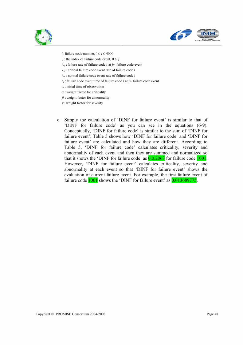
e. Simply the calculation of ‘DINF for failure event’ is similar to that of
‘DINF for failure code’ as you can see in the equations (6-9). Conceptually, ‘DINF for failure code’ is similar to the sum of ‘DINF for failure event’. Table 5 shows how ‘DINF for failure code’ and ‘DINF for failure event’ are calculated and how they are different. According to Table 5, ‘DINF for failure code’ calculates criticality, severity and abnormality of each event and then they are summed and normalized so that it shows the ‘DINF for failure code’ as 0.0.2063 for failure code 1001. However, ‘DINF for failure event’ calculates criticality, severity and abnormality at each event so that ‘DINF for failure event’ shows the evaluation of current failure event. For example, the first failure event of failure code 1001 shows the ‘DINF for failure event’ as 0.013689775.

Copyright © PROMISE Consortium 2004-2008 Page 49
@
Table 5. Comparison between ‘DINF for failure code’ and ‘DINF for failure event’
Step 6. Calculate coefficient by DSS
a. With ‘DINF for failure event’ and environmental operating data from PDKM, this procedure makes multi linear regression models and solve it to calculate coefficient between DINF for failure event and environmental operating data.
b. The multi linear regression is calculated based on the following model.
,1 1,1 ,1
,2 1,1 ,2
,
k m
k m
k n
B AXDINF for failure code event environmental data environmental dataDINF for failure code event environmental data environmental data
DINF for failure code event e
=
⎛ ⎞⎜ ⎟⎜ ⎟ =⎜ ⎟⎜ ⎟⎝ ⎠
L
L
M M
1
2
1, , n m n m
coefficientcoefficient
nvironmental data environmental data coefficient
⎛ ⎞⎛ ⎞⎜ ⎟⎜ ⎟⎜ ⎟⎜ ⎟⎜ ⎟⎜ ⎟⎜ ⎟⎜ ⎟⎝ ⎠⎝ ⎠
M
L
: : :
k failure code numberm environmental data numbern the number of failure code event
i. The coefficient is the regression coefficient between DINF for failure code event and environmental operating data .
ii. The calculation example is described in the following tables. * Field data sample
Field data
DINF for failure code
Failure code Failure code event rate
Criticality for failure event Criticality for fcode Abnormality of failure
event Abnormality for fcode
Severity of failure event
Severity for fcode
DINF for failure code
2.31481E-05 0.004976852 2.21481E-05 5.35837E-10 4.2735E-05 0.004957265 4.1735E-05 5.4408E-09
5.95238E-05 0.004940476 5.85238E-05 2.33177E-09 1001
4.62963E-05 0.004953704
0.991414835
4.52963E-05
0.008386842
0
0.003681 0.020653
2.31481E-05 0.004976852 2.21481E-05 5.35837E-10 3.96825E-05 0.004960317 3.86825E-05 2.29644E-09 5.55556E-05 0.004944444 5.45556E-05 4.40917E-09
1002
3.96825E-05 0.004960317
0.992096561
3.86825E-05
0.00770498
0
0.002018 0.017627
DINF for failure event
Failure code
Failure code event rate
Criticality for failure event
Abnormality for failure event
Severity for failure event
DINF for failure event
2.31481E-05 0.99537037 0.004430516 0.00462963 0.013689775 4.2735E-05 0.991452991 0.008348678 0.003917379 0.020813066
5.95238E-05 0.988095238 0.011707103 0.003357753 0.026969619 1001
4.62963E-05 0.990740741 0.009061071 0 0.018320331 2.31481E-05 0.99537037 0.004430516 0.00462963 0.013689775 3.96825E-05 0.992063492 0.007738056 0.003306878 0.018981442 5.55556E-05 0.988888889 0.010913294 0.003174603 0.025199008
1002
3.96825E-05 0.992063492 0.007738056 0 0.015674563
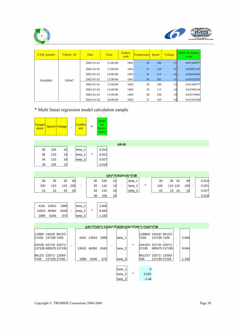
Copyright © PROMISE Consortium 2004-2008 Page 50
@
FAM_number Vehicle_ID Date Time Failure code Temperature Speed Voltage DINF for failure
event
2002-01-01 12:00:00 1001 30 100 15 0.01368977
2002-01-01 13:00:00 1001 35 110 13 0.02081307
2002-01-01 14:00:00 1001 34 115 16 0.02696962
2002-01-02 12:00:00 1001 30 105 15 0.01832033
2002-01-01 12:00:00 1002 30 100 15 0.01368977
2002-01-01 14:00:00 1002 34 115 16 0.01898144
2002-01-01 15:00:00 1002 30 100 14 0.02519901
MA00001 185047
2002-01-02 16:00:00 1002 31 105 16 0.01567456
* Multi linear regression model calculation sample
Temperature Speed Voltage . Coeffici
ent = DINF
for failure event
AX=B 30 100 15 beta_1 0.014 35 110 13 beta_2 0.021 34 115 16
.
beta_3
=
0.027
30 105 15 0.018
{(A)^(T)A}X=(A)^(T)B 30 35 34 30 30 100 15 beta_1 30 35 34 30 0.014
100 110 115 105 35 110 13 beta_2 100 110 115 105 0.02115 13 16 15
.
34 115 16
.
beta_3
=
15 13 16 15
.
0.027
30 105 15 0.018
4181 13910 1899 beta_1 2.606 13910 46350 6345 beta_2 8.684
1899 6345 875
.
beta_3
=
1.182
{(A)^(T)A}^(-1){(A)^(T)A}X={(A)^(T)A}^(-1)(A)^(T)B
11889/27439
-24419/137195
9612/27439 4181 13910 1899 beta_1
11889/27439
-24419/137195
9612/27439 2.606
-24419/137195
52174/685975
-22671/137195 13910 46350 6345 beta_2
-24419/137195
52174/685975
-22671/137195 8.684
9612/27439
-22671/137195
12050/27439
.
1899 6345 875
.
beta_3
=
9612/27439
-22671/137195
12050/27439
.
1.182 beta_1 -0 beta_2 0.001 beta_3
=
-1.46

Copyright © PROMISE Consortium 2004-2008 Page 51
@
** DINF for failure event = -0.002391065*temperature + 0.001307982*speed + -1.455646013*voltage
iii. According to the sample calculation, the change of the DINF for failuire event is much affected by the voltage negatively, which means that the occurrence of failue code 1001 incresases according to the decrease of voltage or vise versa.
c. The objective of ‘Calculate coefficient by DSS’ is to provide DfX specialist engineer with the correlation between the change of failure code event rate and environmental operating data. From the calculation result of multi linear regression model, the higher or lower coefficient of environmental operating data compared to other coefficient indicates that these environmental operating data has much correlated with the change of failure code event rate. The positive number means that the failure code event rate increases as environmental operating data increases or vise versa. Hence, DfX specialist engineer can find which environmental operating data affects the change of failure code event rate based on the coefficient values.
Table 6. Coefficient calculation result
vehicle_id Failure code
Laufleistung (Mileage)
(km)
Fahrdrahtspannung(Line
_voltage) (volt)
Fahrdrahtstrom
(Line_current)
(ampere)
Filterstrom (Filter_curre
nt) (ampere)
Heizspannung
(Heating_circuit_current)
(ampere)
Lokbeschleunigung
(Vehicle_acceleration)
(m/s²)
Istwert_HL_Druck
(Actual_HL_pressure)
(bar)
185047 1024 7.34E-10 1.35E-05 1.78E-06 -1.11E-06 3.05E-06 3.79E-05 -3.19E-05185047 1026 1.78E-09 1.64E-05 5.19E-07 7.55E-08 3.30E-06 -1.20E-04 6.46E-05185047 1027 0 0 0 0 0 0 0185047 1092 0 0 0 0 0 0 0185047 1095 0 0 0 0 0 0 0185047 1099 0 0 0 0 0 0 0185047 1147 0 0 0 0 0 0 0185047 1148 0 0 0 0 0 0 0185047 1150 0 0 0 0 0 0 0185047 1154 0 0 0 0 0 0 0185047 1190 1.10E-08 1.84E-05 -3.27E-07 3.83E-06 -1.52E-05 2.00E-04 7.11E-05185047 1191 6.06E-09 1.48E-05 -1.30E-07 4.49E-07 -9.09E-06 1.43E-04 1.32E-04185047 1200 4.87E-09 1.24E-05 -2.03E-07 1.64E-06 -1.23E-05 3.73E-04 1.11E-04185047 1201 0 0 0 0 0 0 0185047 1202 0 0 0 0 0 0 0185047 1203 0 0 0 0 0 0 0185047 1204 0 0 0 0 0 0 0185047 1248 -5.20E-10 8.38E-06 -1.29E-06 -1.92E-07 1.14E-06 -3.46E-05 -4.20E-06185047 1249 -4.84E-10 6.82E-06 -1.43E-07 6.20E-08 1.43E-06 4.48E-06 1.29E-06185047 1251 -4.84E-10 6.82E-06 -1.43E-07 6.20E-08 1.43E-06 4.48E-06 1.29E-06
d. The high value of coefficient means that environmental operating data is
much correlated with the change of failure code event rate of the selected failure code, which indicates that if the environmental operating data changes, then failure code event rate also changes according to the environmental operating data changes.

Copyright © PROMISE Consortium 2004-2008 Page 52
@
e. The absolute value of coefficient is not significant. The relative comparison of coefficient values among environmental operating data has meaning in multi linear regression model. For example in Table 6, failure code 1024 is affected negatively by Filterstrom (Filter_current) (-1.11E-06). Failure code 1024 is also much affected by Lokbeschleunigung (Vehicle_acceleration) (3.79E-05). Fahrdrahtspannung (Line_voltage) (1.35E-05) has more effect on failure code event rate than Laufleisung (7.34E-10).
f. In Table 6, some failure codes (1026, 1027, ….) have no result of coefficient calculation since there is less failure code event so that multi linear regression model can not be established.
g. Following Figure 27 shows that coefficient of environmental operating data according to failure code. In this graph, each line indicates failure and the coefficient axis indicates the amount of coefficient according to environmental operating data. According to the Figure 27, the failure code ‘4014’ is much affected by ‘Istwert HL druck’ negatively.
Figure 27. Coefficient of environmental operating data to failure code event rate
Step 7. Start clustering by DfX specialist engineer
a. If DfX specialist engineer wants to group the environmental operating data which has similar values, DfX specialist engineer can start clustering procedure.
b. The clustering of environmental operating data shows how the value of environmental operating data is scattered and how the scattered data can be grouped as clusters.
c. Clustering is performed in two ways.

Copyright © PROMISE Consortium 2004-2008 Page 53
@
i. The first one is clusters for each environmental operating data, which is called single clustering. The clusters in this procedure are grouped by the value of each environmental operating data field having similar values.
ii. The second one is clusters for failure event. The clusters in this procedure contain failure events which have similar environmental operating data set. To do this, the environmental operating data set is defined as the multi dimension vector where each environmental operating data becomes different dimension separately. Then, the euklid distance between each environmental operating data vector are calculated. The environmental operating data vectors having similar distance are grouped and made as clusters.
d. In the clustering procedure, we use not mean, min, max and etc but each environmental operating data per failure event from PDKM.
Step 8. Make single clustering by DSS
a. The objective of single clustering is to make clusters for each environmental operating data respectively. Hence, from the result of single clustering, DfX specialist engineer can recognize how data in each environmental operating data is spread.
Table 7. Single clustering result Cluster 1 Cluster 2 Cluster 3 Cluster 4 MA00334
Mean Variance Min Max Mean Variance Min Max Mean Variance Min Max Mean Variance Min Max Laufleistung (Mileage) 0 0 0 0 44305.1 197.7882 43974 44699 45093.1 166.0513 44702 45476 45860.66 223.809 45484 46471
System 80 0 80 80 Fahrdrahtspannung(Line_
voltage) 0.543505 0.419189 0 5.01961 15.08835 0.331595 13.8039 15.3726 15.69022 0.132044 15.451 15.8431 16.00358 0.063494 15.9216 16.0784Fahrdrahtstrom (Line_current) 2.477399 2.121007 0 7.84314 16.79236 10.30801 11.7647 62.7451 113.3025 35.5703 66.6667 188.235 269.4821 66.06921 192.157 439.216
Filterstrom (Filter_current) 0.820793 3.798669 0 27.451 63.37884 3.897943 35.2941 78.4314 98.45377 15.85217 82.3529 188.235 Heizspannung
(Heating_circuit_current) 0 0 0 0 6.901957 2.226676 5.88235 11.7647 18.26562 16.16162 17.6471 505.882 Heizstrom
(Heating_circuit_current) 0 0 0 0 Lokbeschleunigung
(Vehicle_acceleration) 0.012095 0.121984 -1.1811 0.551181 Istwert_HL_Druck
(Actual_HL_pressure) 0.376167 0.407542 0 1.82677 3.285015 0.310771 1.95276 3.71654 4.157919 0.22458 3.77953 4.59843 5.064906 0.083321 4.66142 5.22835Fahrtrichtung_1
(Driving_direction_1) 0 0 0 0 1 0 1 1 Fahrtrichtung_2
(Driving_direction_2) 0.218776 0.413416 0 1 Fahrertisch_besetzt
(Driver_control_desk_activ) 0.875918 0.329675 0 1
Bremsart_G_Ein (Brake_application_G_On) 0.222857 0.416163 0 1
Bremsart_P_Ein (Brake_application_P_On) 0 0 0 0 1 0 1 1
Druckluft_8_5_Bar (Compressed_air_8_5_Ba
r) 0.158095 0.36483 0 1 Zusatzbremse_Ein
(Supplementary_brake_On) 0 0 0 0 1 0 1 1
Sanden_Ein (Sanding_On) 2.72E-04 0.016493 0 1 LZB_Ein (ATC_On) 0 0 0 0

Copyright © PROMISE Consortium 2004-2008 Page 54
@
b. Since the clusters are made for each environmental operating data, there is no relationship among clustering of each environmental operating data. DfX specialist engineer should check clusters in each environmental operating data. For example, environmental operating data ‘Fahrdrahtspannung(Line_voltage)’ has four clusters in Table 7. In each cluster, there are several values of ‘Fahrdrahtspannung (Line_voltage)’ which are similar and they are calculated as mean and variance. Each cluster has means 0.543505, 15.08835, 15.69022, and 16.00358 which means the data of ‘Fahrdrahtspannung (Line_voltage)’ can be grouped in four clusters according to the similarity of ‘Fahrdrahtspannung (Line_voltage)’ values. This means that ‘Fahrdrahtspannung (Line_voltage)’ values extracted during observation period by FAM are scattered around the calculated mean value 0.543505, 15.08835, 15.69022, and 16.00358. The variance of each cluster is 0.419189, 0.331595, 0.132044, and 0.063494. The min and max values indicate the lowest value and highest value of each cluster.
c. The single clustering is done by each environment operating data separately. Hence, each environmental operating data has different number of clusters according to the values of each environmental operating data. For example in Table 7, Laufleistung (Mileage) has four clusters, Lokbeschleunigung (Vehicle_acceleration) has only one cluster, and Fahrtrichtung_1 (Driving_direction_1) has two clusters.
Figure 28. Graph for single clustering result
d. Figure 28 shows the result of Table 7 as graphical way for one
environmental operating data (Fahrdrahtstrom (Line_current)). According to this figure, Fahrdrahtstrom (Line_current) has four clusters and each cluster has mean and variance (cluster 1 (2.477399, 2.121007), cluster 2 (16.79236, 10.30801), cluster 3 (113.3025, 35.5703), cluster 4 (269.4821, 66.06921)). The radius of circle comes from the variance of each cluster.

Copyright © PROMISE Consortium 2004-2008 Page 55
@
This graph will be modified as 3D to show the number of data in each cluster by Z axis.
Cluster
Voltage
# of cluster elements
1 2 3
40
80
120
50
100
150
Cluster
Voltage
# of cluster elements
1 2 3
40
80
120
50
100
150
Figure 29. Different type of graph for single clustering result
e. Figure 29 shows the diffent type of graph for single clustering result. This
graph shows one more information about the number cluster elements in z-axis.
Step 9. Make multiple clustering by DSS
a. The objective of ‘Make multiple clustering by DSS’ is to provide the groups of failure code events which have similar environmental operating data set.
b. Each failure code event has several kinds of environmental operating data and the clusters are made by considering all environmental operating data concurrently for each failure code event. In the multiple clustering, all the environmental operating data are used as sets in clustering of failure code event. If the failure code events have similar environmental operating data sets, then they will be grouped together and made as clusters.
c. In the multiple clustering, the elements in clusters are failure code events which are grouped by all environmental operating data recorded whent the failure code events happen.
d. From the ‘Make multiple clustering by DSS’, DfX specialist engineer can recognize the environmental status and operating status having similar environmental operating data set.
e. According to Table 8, cluster 1 shows environmental status which has the means of each environmental operating data such as System (80.15664), Fahrdrahtspannung(Line_voltage) (2.379417), Fahrdrahtstrom (Line_current) (5.791101), Filterstrom (Filter_current) (9.637),

Copyright © PROMISE Consortium 2004-2008 Page 56
@
Heizspannung (Heating_circuit_current) (2.397011), Heizstrom (Heating_circuit_current) (0), Lokbeschleunigung (Vehicle_acceleration) (0.006301), Istwert_HL_Druck (Actual_HL_pressure) (3.82879), Fahrtrichtung_1 (Driving_direction_1) (0.61521), Fahrtrichtung_2 (Driving_direction_2) (0.06924), Fahrertisch_besetzt (Driver_control_desk_activ) (0.766175), Bremsart_G_Ein (Brake_application_G_On) (0.083995), Bremsart_P_Ein (Brake_application_P_On) (0.354143), Druckluft_8_5_Bar (Compressed_air_8_5_Bar) (0.297389), Zusatzbremse_Ein (Supplementary_brake_On) (0.602724), Sanden_Ein (Sanding_On) (0), and LZB_Ein (ATC_On) (0). The variance is calculated in Table 8.
f. Figure 30 shows the result of Table 8 in graphical way.
Figure 30. Graph for multi clustering result
g. This spider web graph shows the overlapped clusters by the mean of each
environmental operating data. Each straight line indicates the environmental operating data and circles means the value of each environmental operating data.

Copyright © PROMISE Consortium 2004-2008 Page 57
@
Table 8. Multi clustering result
Clu
ster
1
Clu
ster
2
Clu
ster
3
Clu
ster
4
Clu
ster
5
Clu
ster
6
Clu
ster
7
Clu
ster
8
Clu
ster
9
Clu
ster
10
Clu
ster
11
Clu
ster
12
Clu
ster
13
Clu
ster
14
Clu
ster
15
Clu
ster
16
Clu
ster
17
Clu
ster
18
System 80.15664 80.04839 80 80 80 80 83.01982 80 80 80 80 80 80 80 80 80 80 80
Fahrdrahtspannung(Line_voltage) 2.379417 13.25792 9.189477 5.973338 16.8539 16.91352 19.56225 15.62937 16.72482 6.110369 16.16707 14.26397 16.22822 15.86158 15.39693 15.41759 15.95331 15.74113Fahrdrahtstrom (Line_current) 5.791101 45.39848 0 0 194.9417 15.51729 16.51981 15.28735 8.624447 0.093573 17.73231 163.3456 27.34235 25.91455 23.98792 25.01039 16.12201 24.64199
Filterstrom (Filter_current) 9.637 58.53891 0.112045 0.427807 98.66438 90.86706 168.5151 81.41317 85.77574 0.20416 83.02494 114.8255 86.62216 60.21364 60.28535 60.26015 62.24712 63.71448Heizspannung
(Heating_circuit_current) 2.397011 5.882352 0.504203 1.604278 6.649613 13.17379 113.1705 12.9209 13.85621 0.1914 9.703631 2.846705 13.6386 11.23794 9.838995 9.8594 9.243708 10.45937
Heizstrom (Heating_circuit_cu
rrent) 0 0 0 0 0 0 6.01652 0 0 0 0 0 0 0 0 0 0 0Lokbeschleunigun
g (Vehicle_accelerati
on) 0.006301 0.01143 0.001125 0.002863 0.230514 0.102292 0.004466 -0.00292 0.00718 0.003331 0.026582 0.101671 -0.00949 0.047156 0.018142 0.018321 0.054993 0.049766Istwert_HL_Druck
(Actual_HL_pressure) 3.82879 4.805181 4.454443 4.274302 4.627638 4.613354 4.412501 4.456584 4.560437 3.927648 4.931429 4.182029 4.882676 4.57492 4.647726 4.41426 4.881389 4.465362
Fahrtrichtung_1 (Driving_direction_
1) 0.61521 0.701613 0.114286 0.309091 0.318841 0.376426 0.222467 0.72069 0.603065 0.418655 0.762148 0.824411 0.32964 0.511194 0.57359 0.487977 0.563492 0.629213Fahrtrichtung_2
(Driving_direction_2) 0.06924 0.165323 0.371429 0.254545 0.637681 0.491762 0.527533 0.134483 0.216858 0.106291 0.173913 0.09636 0.584488 0.268657 0.232462 0.356436 0.230159 0.148876
Fahrertisch_besetzt
(Driver_control_desk_activ) 0.766175 0.927419 0.657143 0.781818 1 0.945501 0.922907 0.839655 0.652874 0.472885 0.928389 0.368308 0.952909 0.899254 0.917469 0.92645 0.912698 0.907303
Bremsart_G_Ein (Brake_application
_G_On) 0.083995 0 0 0 0 0 0 0.137931 0 0 0 0.029979 0 0.108209 0.170564 0.118812 0.111111 0.061798Bremsart_P_Ein
(Brake_application 0.354143 0 0 0 0 0 0.759912 0.010345 0.081226 0 0 0 0 0.891791 0.460798 0.881188 0.888889 0.738764

Copyright © PROMISE Consortium 2004-2008 Page 58
@
_P_On) Druckluft_8_5_Bar (Compressed_air_8
_5_Bar) 0.297389 0.22379 0.028571 0.145455 0.304348 0.069708 0.227974 0.074138 0.067433 0.067245 0.035806 0.040685 0.022161 0.13806 0.137552 0.179632 0.079365 0.11236Zusatzbremse_Ein (Supplementary_br
ake_On) 0.602724 0.580645 1 0.909091 0.724638 0.461343 0.313877 0.401724 0.394636 0.813449 0.613811 0.40257 0.429363 0.485075 0.473177 0.567185 0.349206 0.41573Sanden_Ein
(Sanding_On) 0 0 0 0 0 0.001267 0 0 0 0 0.005115 0 0 0 0.001376 0 0 0LZB_Ein (ATC_On) 0 0 0 0 0 0 0 0 0 0 0 0 0 0 0 0 0 0

Copyright © PROMISE Consortium 2004-2008 Page 1
@
h. However, if the clusters have different mean value of environmental operating data
compared to other cluster such as ‘Filterstrom (Filter_current)’ in yellow line of cluster 7 in the spider web, then the failure events in cluster 7 has higher mean value of ‘Filterstrom (Filter_current)’ (168.5151) than mean value of ‘Filterstrom (Filter_current)’ of other clusters. This means cluster 7 has different environment status compared to other clusters.
i. The mean of ‘Heizspannung (Heating_circuit_current)’ in cluster 7 also shows different range of mean from other clusters. Other clusters except cluster 7 have similar mean value of ‘Heizspannung (Heating_circuit_current)’ around zero. However, the mean of ‘Heizspannung (Heating_circuit_current)’ in cluster 7 has high mean value of ‘Heizspannung (Heating_circuit_current)’ around 113.1795.
j. According to the Figure 30, the cluster 7 seems to have different environmental status, specially ‘Filterstrom (Filter_current)’ and ‘Heizspannung (Heating_circuit_current)’. Cluster 5 shows much different environment in ‘Fahrdrahtstrom (Line_current)’ (194.9417) compared to other clusters.
3.4 GUI development This section gives a short overview on the current state of the graphical user interface (GUI) developed for the BT application scenario. As described in the previous sections of the deliverable, a clustering-based DSS algorithm has been specifically developed by EPFL for the analysis of the locomotive data provided by Bombardier. In particular, the different analysis steps required by the algorithm have been identified, together with their parameters. This results in a set of mockups for the GUI. The mockups have been developed by EPFL and iterated with Bombardier to reach its final version. Like other demonstrators in the PROMISE project, the real DSS GUI for the Bombardier’s demonstrator has been developed on the basis of the provided mockups. The single screens of the GUI were implemented exactly according to the design specified in the mockups. SAP Portal technologies (WebDynPro) were utilized so that the DSS GUI can be easily integrated with the GUI of the PDKM implemented in Workpackage R10 (led by InMediasP). This is mandatory in order to achieve with the PDKM a uniform platform for PLM as well as DSS functions. The general web-service-based approach to the communication between the GUI and the logic of the DSS was already described in detail in Section 4 of Deliverable DR 10.4. The current implementation of the DSS GUI for the BT scenario has been integrated and deployed into the PDKM for demonstration purposes. It is to be found under the section of BOL functions in the PDKM. The BT scenario represents the single BOL scenario among all PROMISE scenarios. All other scenarios are integrated under the sections MOL and EOL functions of the PDKM, respectively. A detailed walkthough of the implemented GUI screens is given in Appendix A. In the BT DSS GUI, we briefly describe the interactions supported by the current implementation of the DSS user interface for the BT scenario. The user interface supports a guided procedure that guides the user through the single steps from data selection to analysis results, i.e. the clusters of similar data. Using the identified clusters, user can identify some particular trends in the operation of the locomotive components of interest. In Appendix A, we give a short walkthrough of the complete user interface. In particular, each of the steps is briefly described and illustrated with a expected screen shot. Please note, that the current DSS of the BT scenario still does not contain application data. The screens thus aim at only giving a real look and feel of the system and illustrating the possible interaction.

Copyright © PROMISE Consortium 2004-2008 Page 2
@
4 Conclusions
4.1 BT demonstrator development For the implementation of BT demonstrator, several partners have worked according to their responsibilities in the defined tasks of DA10.6. The implementation of BT demonstrator can be divided into the following five main parts. During the development of BT demonstrator, several problems have been identified and appropriate solutions have been proposed and implemented.
• Field data transfer from BT database to PDKM o The huge size of BT field data is one of main issues. The capacity of PDKM which
is provided by SAP is not sufficient to contain all BT field data and not all data is necessary for the BT DSS. To resolve this problem, BT, EPFL, and InMediasP decide to reduce the data size as much as necessary for DSS algorithm. Based on the agreement between BT, EPFL, and InMediasP, the sort of field data and the amount of field data is defined and applied into BT DSS.
• Data access to PDKM by Cognidata • BT DSS development by EPFL
o The algorithm of BT DSS is changed during the development of BT DSS according to the new user requirements. New conceptual procedure such as statistical method is added in updated version of BT DSS.
• DSS GUI development by SAP o According to the change of BT DSS, BT DSS GUI is changed so as to apply new
user requirements. • Integration
o Currently, each part of BT DSS demonstrator is implemented except the integration into the PROMISE PDKM. The integration of BT DSS demonstrator needs some further work among the involved partners. This is a time consuming work and will be accomplished following the overall plan for the implementation of the PROMISE demonstrators. The remaining work will be completed in the industrialisation phase of the BT DSS demonstrator presented in the next session.
4.2 Industrialization of BT demonstrator development The task of combining field information gained by the operation of locomotives given as ‘failure data’ and ‘diagnostics data’ to create knowledge showed up to be far more complex than intended in the beginning of the project. The reason was not primarily the challenging task of developing the DSS algorithm itself, but the plain amount of data to be checked, cleaned and processed. As shown in chapter 2.1.4 the original data provided by Bombardier Transportation (considered necessary to get statistically sound information) and transferred to the project partners, contained about 4,2 billion individual field data. For reasons given in 2.1.4 the amount of data had to be cut down to about 2 million data sets for developing and testing the DSS/DfX. This step was agreed by the A10 working team. The consequences of this data cut were: - restrictions in the selection of the components to be considered (down to one single kind of
component)

Copyright © PROMISE Consortium 2004-2008 Page 3
@
- restrictions of the failure reports and the related diagnostics data - restrictions of the time span covered by the analysis
These restrictions led to limitations of the evaluation of the results of the Promise A10 WP; i.e. on the practical technical/engineering significance of the outcome and limited answers on questions of algorithm performance etc. As far as the DfX demonstrator is a prototype, it does not yet allow an economic evaluation. Nevertheless, this does not restrict conclusions on the principal applicability of the chosen DSS/DfX process and the possible reuse of algorithms. To the extent to which the above mentioned restrictions allow, the developed algorithm proved to be appropriate as a fast and easy to adopt first approach analysis tool. There are no restrictions to the applicability of other (in fact unrestricted) components. There is a great potential for further development and refinement with the main focus on implementing the algorithm in a working environment which fulfil the needs of a daily industrial application. So a possible way forward should be - finalization of the data management process (optimization of the integration of the underlying
database and the adaption of the GUI to specific needs). - consideration of other applications using the capability of extended data management for a
more accurate evaluation - detailed testing on the basis of the enhanced DfX after the end of the project - optimization of the selection of data provided by the applicator (concerning the parameters
monitored on board of the locomotives) - optimization of the data management process by pre-processing and combining data on board
of the locomotives - transfer the developed DfX prototype tools into a robust and commercially usable tool
5 References [1] DA10.3: Design of the BT DfX Demonstrator on BOL [2] DR 8.3: Specification of the PROMISE DSS prototype (Version 1) [3] DA10.1: Scope definition and description of current state vs. critical issues [4] DR3.2 - PROMISE Demonstrators [5] DR8.1 - Design of the decision support system [6] Bombardier Transportation field data: FAM 07_2001 bis 05_2006.xls [7] Bombardier Transportation diagnostics data table: DDSUMFLD.xls [8] Bombardier Transportation diagnostics data table: ERROR_CODE.xls [9] Bombardier Transportation diagnostics data table: HEADER.xls [10] Bombardier Transportation document: Struktur_Zentrale_Diagnosedatenbank.doc [11] PROMISE Consortium Cooperation Agreement FP6-2002-IST-NMP

Copyright © PROMISE Consortium 2004-2008 Page 4
@
Appendix A. BT DSS GUI
FAM Selection
FAM Selection
Input period to search FAM
YYYY / MM / DD ~ YYYY / MM / DD
Select FAM
Available FAM list
FAM NUMBER Database Name Date ------- CommentMA00334 DB2 name02 2002/06/03 ------- broken-------- -------- -------- -------- ------- --------
MA00431 DB2 name06 2002/06/03 ------- failed
Search!
DSS parameters
DSS parameters
Parameters input
Parameters for DINF calculationNormal failure rateCritical failure rateWeight factor of criticalityWeight factor of abnormalityWeight factor of severity
Parameters for clusteringCluster add factor

Copyright © PROMISE Consortium 2004-2008 Page 5
@
3. DINF calculation
Run DINF calculation
Run clustering
4. Failure code selection
DINF calculation result and failure code selection
Failure codes by DINF order
Select failure code
Failure code criticality abnormality Severity DINF RANK4014 0.8 0.7 0.5 0.9 1
------ ------ ------ ------ ------ ------
------ ------ ------ ------ ------ ------
0.1 0.1 1903014 0.1 0.1

Copyright © PROMISE Consortium 2004-2008 Page 6
@
4.1 Visualization
Visualization input matrix
criti
calit
y fo
rfc
ode
seve
rity
for
fcod
e
3995
39850
0.020.040.060.080.1
0.120.14
Failure code
DINF calculation result
39954014398439854005
5. Coefficient calculation
Run coefficient calculation
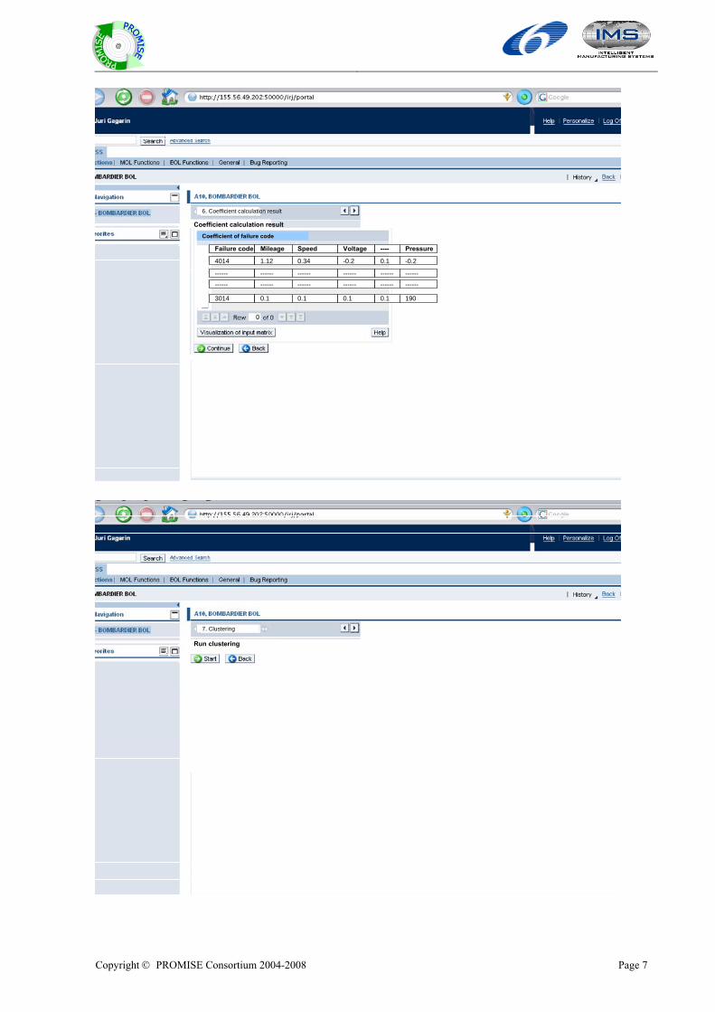
Copyright © PROMISE Consortium 2004-2008 Page 7
@
6. Coefficient calculation result
Coefficient calculation resultCoefficient of failure code
Failure code Mileage Speed Voltage ---- Pressure
4014 1.12 0.34 -0.2 0.1 -0.2
------ ------ ------ ------ ------ ------
------ ------ ------ ------ ------ ------
0.1 0.1 1903014 0.1 0.1
7. Clustering
Run clustering

Copyright © PROMISE Consortium 2004-2008 Page 8
@
8. Single clustering result
Single clustering resultClustering of field data
FAM Cluster 1
Mileage 100 99
Max Min Avg Var----
Max Min Avg VarCluster 10
Max Min Avg Var
98 1 ----- ---------- ----- 190 187185 2
MA00334
Speed 80 7978 2 ----- ---------- ----- 100 9998 3
Voltage 2 1.91.8 0.2 ----- ---------- ----- 1.2 0.90.8 0.1
---- ---- -------- ---- ----- ---------- ----- ---- -------- ----
8.1 Visualization
Visualization input matrix
Cluster
Voltage
# of cluster elements
1 2 3
40
80
120
50
100
150

Copyright © PROMISE Consortium 2004-2008 Page 9
@
9. Multi clustering result
Multi clustering resultClustering of failure event
Failure event Cluster 1
Mileage 100 99
Max Min Avg Var----
Max Min Avg VarCluster 10
Max Min Avg Var
98 1 ----- ---------- ----- 190 187185 2
Speed 80 7978 2 ----- ---------- ----- 100 9998 3Voltage 2 1.91.8 0.2 ----- ---------- ----- 1.2 0.90.8 0.1
---- ---- -------- ---- ----- ---------- ----- ---- -------- ----
9.1 Visualization
Visualization input matrix
Multi clustering
-50
0
50
100
150
200System
Fahrdrahtspannung
Fahrdrahtstrom
Filterstrom
Heizspannung
Heizstrom
Lokbeschleunigung
Istwert_HL_Druck
Fahrtrichtung_1Fahrtrichtung_2
Ferertisch_besetzt
Bremsart_G_Ein
Bremsart_P_Ein
Druckluft_8_5_Bar
Zusatzbremse_Ein
Sanden_Ein
LZB_Ein
Cluster 1 MeanCluster 2 MeanCluster 3 MeanCluster 4 MeanCluster 5 MeanCluster 6 MeanCluster 7 MeanCluster 8 MeanCluster 9 MeanCluster 10 MeanCluster 11 MeanCluster 12Cluster 13Cluster 14Cluster 15Cluster 16Cluster 17Cluster 18


![Controlador de motor CMMS-AS/CMMS-ST/CMMD-AS · Descripción Funcionesy puesta apunto Versióndefirmware apartirde1.4.0.x.6 8040107 1404NH [8034521] Controlador de motor CMMS-AS/CMMS-ST/CMMD-AS](https://static.fdocuments.in/doc/165x107/60267df4bc18d8032670fb49/controlador-de-motor-cmms-ascmms-stcmmd-as-descripcin-funcionesy-puesta-apunto.jpg)