D. Numerical experiments for tropical cyclones D-1. …€¦ · global analysis (GA) and the global...
44
TECHNICAL REPORTS OF THE METEOROLOGICAL RESEARCH INSTITUTE No.65 2012 D. Numerical experiments for tropical cyclones D-1. Forecast experiment with a nonhydrostatic model and simulation of storm surge on cyclone Nargis 1 D-1-1. Introduction Severe meteorological phenomena such as tropical cyclones (TCs) sometimes cause catastrophic damage to human society; therefore, their prediction is significantly important for preventing and mitigating meteorological disasters. In the areas around the Bay of Bengal, historically, there have been several cases in which storm surges induced by TCs gave rise to severe floods (Webster 2008). At the end of April 2008, cyclone Nargis was generated in the center of the bay and moved eastward in contrast with typical northward motion of cyclone of the bay such as the 1970 Bohla cyclone or the 1991 Bangladesh cyclone. Nargis reached its maximum intensity of category 4 around 06–12 UTC on 2 May, then it made landfall in southern Myanmar, and caused a destructive storm surge over the Irrawaddy Delta and other low-lying areas that claimed more than one hundred thousand lives. Figure D-1-1 shows the development of Nargis estimated by the Regional Specialized Meteorological Center (RSMC) New Delhi and the US Navy Joint Typhoon Warning Center (JTWC). The minimum center pressure by JTWC was 937 hPa, while the RSMC New Delhi estimated its intensity as 962 hPa. For disaster prediction and mitigation in these areas, forecasts of TCs and the associated storm surges based on numerical weather prediction (NWP) are particularly important. In this study, numerical simulations of the 2008 Myanmar cyclone Nargis and the associated storm surge were conducted using the Japan Meteorological Agency (JMA) Nonhydrostatic Model (NHM; Saito et al. 2001; Saito et al. 2006) and the Princeton Ocean Model (POM; Blumberg and Mellor 1987). The JMA operational global analysis (GA) and the global spectral model (GSM) forecast have been operated, but they underestimated Nargis’ intensity probably due to its coarse horizontal resolution (T213) or inaccuracy of initial conditions. We show that downscale experiments by NHM using GA and GSM forecast data reproduced the development of Nargis more properly as bellow. This work also aims to demonstrate the applicability of downscale NWP in Southeast Asia and to propose a decision support for preventing and mitigating meteorological disasters, in view of the recent situation that the numerical simulation models and the data are available and accessible to registered users in Southeast Asia as shown in Section E-3. D-1-2. Cyclone forecast experiments NHM forecast experiments with a horizontal resolution of 10 km were conducted with using GA and GSM forecast data as the initial and the lateral boundary conditions, respectively. The model domain is a square of 3400 km size (1˚S-30˚N, 73˚E-107˚E) which covers the Bay of Bengal and the surrounding areas including Myanmar (Fig. D-1-2). We assumed a minimum lead time of two days before the landfall in order to effectively mitigate Nargis’ storm surge damage and set the initial time of our simulation as 12 UTC on April 30 2008, when Nargis started its eastward movement and one 1 T. Kuroda, K. Saito, M. Kuni and N. Kohno (JMA) - 42 -
Transcript of D. Numerical experiments for tropical cyclones D-1. …€¦ · global analysis (GA) and the global...

TECHNICAL REPORTS OF THE METEOROLOGICAL RESEARCH INSTITUTE No.65 2012
42
D. Numerical experiments for tropical cyclones D-1. Forecast experiment with a nonhydrostatic model and simulation of storm surge on cyclone Nargis1 D-1-1. Introduction
Severe meteorological phenomena such as tropical cyclones (TCs) sometimes cause catastrophic damage to human society; therefore, their prediction is significantly important for preventing and mitigating meteorological disasters. In the areas around the Bay of Bengal, historically, there have been several cases in which storm surges induced by TCs gave rise to severe floods (Webster 2008). At the end of April 2008, cyclone Nargis was generated in the center of the bay and moved eastward in contrast with typical northward motion of cyclone of the bay such as the 1970 Bohla cyclone or the 1991 Bangladesh cyclone. Nargis reached its maximum intensity of category 4 around 06–12 UTC on 2 May, then it made landfall in southern Myanmar, and caused a destructive storm surge over the Irrawaddy Delta and other low-lying areas that claimed more than one hundred thousand lives. Figure D-1-1 shows the development of Nargis estimated by the Regional Specialized Meteorological Center (RSMC) New Delhi and the US Navy Joint Typhoon Warning Center (JTWC). The minimum center pressure by JTWC was 937 hPa, while the RSMC New Delhi estimated its intensity as 962 hPa. For disaster prediction and mitigation in these areas, forecasts of TCs and the associated storm surges based on numerical weather prediction (NWP) are particularly important. In this study, numerical simulations of the 2008 Myanmar cyclone Nargis and the associated storm surge were conducted using the Japan Meteorological Agency (JMA) Nonhydrostatic Model (NHM; Saito et al. 2001; Saito et al. 2006) and the Princeton Ocean Model (POM; Blumberg and Mellor 1987). The JMA operational global analysis (GA) and the global spectral model (GSM) forecast have been operated, but they underestimated Nargis’ intensity probably due to its coarse horizontal resolution (T213) or inaccuracy of initial conditions. We show that downscale experiments by NHM using GA and GSM forecast data reproduced the development of Nargis more properly as bellow. This work also aims to demonstrate the applicability of downscale NWP in Southeast Asia and to propose a decision support for preventing and mitigating meteorological disasters, in view of the recent situation that the numerical simulation models and the data are available and accessible to registered users in Southeast Asia as shown in Section E-3.
D-1-2. Cyclone forecast experiments NHM forecast experiments with a horizontal resolution of 10 km were conducted with using GA and GSM forecast data as the initial and the lateral boundary conditions, respectively. The model domain is a square of 3400 km size (1˚S-30˚N, 73˚E-107˚E) which covers the Bay of Bengal and the surrounding areas including Myanmar (Fig. D-1-2). We assumed a minimum lead time of two days before the landfall in order to effectively mitigate Nargis’ storm surge damage and set the initial time of our simulation as 12 UTC on April 30 2008, when Nargis started its eastward movement and one
1 T. Kuroda, K. Saito, M. Kuni and N. Kohno (JMA)
- 42 -

TECHNICAL REPORTS OF THE METEOROLOGICAL RESEARCH INSTITUTE No.65 2012
42
D. Numerical experiments for tropical cyclones D-1. Forecast experiment with a nonhydrostatic model and simulation of storm surge on cyclone Nargis1 D-1-1. Introduction
Severe meteorological phenomena such as tropical cyclones (TCs) sometimes cause catastrophic damage to human society; therefore, their prediction is significantly important for preventing and mitigating meteorological disasters. In the areas around the Bay of Bengal, historically, there have been several cases in which storm surges induced by TCs gave rise to severe floods (Webster 2008). At the end of April 2008, cyclone Nargis was generated in the center of the bay and moved eastward in contrast with typical northward motion of cyclone of the bay such as the 1970 Bohla cyclone or the 1991 Bangladesh cyclone. Nargis reached its maximum intensity of category 4 around 06–12 UTC on 2 May, then it made landfall in southern Myanmar, and caused a destructive storm surge over the Irrawaddy Delta and other low-lying areas that claimed more than one hundred thousand lives. Figure D-1-1 shows the development of Nargis estimated by the Regional Specialized Meteorological Center (RSMC) New Delhi and the US Navy Joint Typhoon Warning Center (JTWC). The minimum center pressure by JTWC was 937 hPa, while the RSMC New Delhi estimated its intensity as 962 hPa. For disaster prediction and mitigation in these areas, forecasts of TCs and the associated storm surges based on numerical weather prediction (NWP) are particularly important. In this study, numerical simulations of the 2008 Myanmar cyclone Nargis and the associated storm surge were conducted using the Japan Meteorological Agency (JMA) Nonhydrostatic Model (NHM; Saito et al. 2001; Saito et al. 2006) and the Princeton Ocean Model (POM; Blumberg and Mellor 1987). The JMA operational global analysis (GA) and the global spectral model (GSM) forecast have been operated, but they underestimated Nargis’ intensity probably due to its coarse horizontal resolution (T213) or inaccuracy of initial conditions. We show that downscale experiments by NHM using GA and GSM forecast data reproduced the development of Nargis more properly as bellow. This work also aims to demonstrate the applicability of downscale NWP in Southeast Asia and to propose a decision support for preventing and mitigating meteorological disasters, in view of the recent situation that the numerical simulation models and the data are available and accessible to registered users in Southeast Asia as shown in Section E-3.
D-1-2. Cyclone forecast experiments NHM forecast experiments with a horizontal resolution of 10 km were conducted with using GA and GSM forecast data as the initial and the lateral boundary conditions, respectively. The model domain is a square of 3400 km size (1˚S-30˚N, 73˚E-107˚E) which covers the Bay of Bengal and the surrounding areas including Myanmar (Fig. D-1-2). We assumed a minimum lead time of two days before the landfall in order to effectively mitigate Nargis’ storm surge damage and set the initial time of our simulation as 12 UTC on April 30 2008, when Nargis started its eastward movement and one
1 T. Kuroda, K. Saito, M. Kuni and N. Kohno (JMA)
43
day before its rapid development. As a result, the minimum sea-level pressure of the experiment was 974 hPa while that of GSM was 993 hPa (Fig. D-1-3), which implied that NHM could predict Nargis’ rapid development more accurately than GSM. The higher resolution of NHM contributed to the better representation of the cyclone center. Another possible cause is the difference in the physical processes, especially the convective parameterization schemes. The Kain–Fristch (K–F) scheme (Kain and Fritsch 1993) employed in NHM tends to heat the atmosphere at lower levels than does the Arakawa-Schubert (A-S) scheme in GSM (Shindo et al. 2008), which would enhance the intensification of Nargis. With respect to the cyclone center position at the landfall time, positional lag of NHM (124 km) was smaller than that in GSM (193 km), although the forecasted track of NHM deviated northwardly from the best track. The maximum surface wind speed predicted by GSM was less than 20 m/s, while that predicted by NHM was more than 30 m/s. Moreover, the NHM forecast well captured Nargis’ characteristics of the compact central dense overcast (CDO) with spiral rainbands to the west and south observed by the Tropical Rainfall Measuring Mission’s Microwave Imager (TRMM/TMI) (Fig. D-1-4). Sensitivity experiments were conducted to investigate the effects of ice phase, sea surface temperature (SST), and horizontal resolutions to Nargis’ rapid development. In a warm rain experiment, Nargis developed earlier and the eye radius became larger than the case with ice phase. As for the SST experiment, it was shown that a high SST anomaly preexistent in the Bay of Bengal led to the rapid intensification of the cyclone, and that SST at least warmer than 29 °C was necessary for the development seen in the experiment. In a simulation with a horizontal resolution of 5 km, the cyclone exhibited more distinct development and attained a center pressure of 968 hPa.
Fig. D-1-1. Time sequence of sea level center pressure estimated by the RSMC New Delhi and JTWC. After Kuroda et al. (2010).
- 43 -

TECHNICAL REPORTS OF THE METEOROLOGICAL RESEARCH INSTITUTE No.65 2012
44
Fig. D-1-2. Domain used for NHM forecasts with the 10 km horizontal resolution. Dotted square is the domain of nested experiment with a horizontal resolution of 5 km, and broken rectangle indicates the domain of POM for storm surge simulations. After Kuroda et al. (2010).
Fig. D-1-3. Time evolution of sea level center pressure of Nargis by NHM (GAGSM) and GSM forecasts. Initial time is 12 UTC 30 April 2008. After Kuroda et al. (2010).
Fig. D-1-4. a) Rainfall rate (mm/hr) observed by TRMM/TMI at 0137 UTC 2 May 2008. After JAXA/EORC Tropical Cyclone Database (http://sharaku.eorc.jaxa.jp/TYP_DB/index_e.shtml). b) Rainfall rate (mm/hr) simulated by NHM at FT=33. After Kuroda et al. (2010).
a) b)
- 44 -

TECHNICAL REPORTS OF THE METEOROLOGICAL RESEARCH INSTITUTE No.65 2012
44
Fig. D-1-2. Domain used for NHM forecasts with the 10 km horizontal resolution. Dotted square is the domain of nested experiment with a horizontal resolution of 5 km, and broken rectangle indicates the domain of POM for storm surge simulations. After Kuroda et al. (2010).
Fig. D-1-3. Time evolution of sea level center pressure of Nargis by NHM (GAGSM) and GSM forecasts. Initial time is 12 UTC 30 April 2008. After Kuroda et al. (2010).
Fig. D-1-4. a) Rainfall rate (mm/hr) observed by TRMM/TMI at 0137 UTC 2 May 2008. After JAXA/EORC Tropical Cyclone Database (http://sharaku.eorc.jaxa.jp/TYP_DB/index_e.shtml). b) Rainfall rate (mm/hr) simulated by NHM at FT=33. After Kuroda et al. (2010).
a) b)
45
D-1-3. Storm surge simulation Numerical experiments on the storm surge were performed with POM with a horizontal resolution of 3.5 km. Oceanic currents and water levels were calculated with sigma (terrain-following) coordinates using the surface pressure and winds from NWP models. The open-sea boundary was assumed to follow a static balance with the atmospheric surface pressure, and deviations from the statically balanced level caused inflow or outflow current and gravitational waves. The astronomical tide was not taken into account, and thus, only the deviation of water level was computed with respect to the ocean’s vertical motion. We conducted simulations by POM using surface pressure and wind fields from the GSM and the NHM forecasts. An experiment with POM using GSM forecast could not reproduce the storm surge (Fig. D-1-5c), while a simulation using NHM forecast predicted a realistic rise in the sea surface level by over 3 m (Fig. D-1-5f) at the Irrawaddy point (Fig. D-1-6). The rise was roughly of the same magnitude as the displacement due to the storm surge at the Yangon River reported by Shibayama et al. (2008), although a simulated maximum rise at the Yangon point (Fig. D-1-6) was 1.5m. In the simulation using NHM forecast, surface wind speeds reached 25 m s-1 (Fig. D-1-5d), and were much higher than those obtained in the GSM forecast which were less than 6 m s-1 (Fig. D-1-5a). Since the sea-level rise due to pressure depression (the inverse barometer effect) was less than 0.5 m, the major part of the storm surge was caused by the ocean current generated by strong wind in the simulation. A southerly sub-surface current driven by strong surface winds of the cyclone caused a storm surge in the river mouths in southern Myanmar facing the Andaman Sea as shown in Fig. D-1-6. We showed that the storm surge produced by Nargis was predictable two days before landfall by a downscale forecast with a mesoscale model using accessible operational NWP data and application of an ocean model.
Fig. D-1-5. a) Time sequence of the surface wind speed by the GSM forecast at the Irrawaddy point (16.10˚N, 95.07˚E). b) Same as in a) but for wind directions. c) Same as in a) but water levels simulated by POM. d)-f) Same as in a)-c) but with the NHM forecast. After Kuroda et al. (2010).
a)
b)
c)
d)
e)
f)
- 45 -

TECHNICAL REPORTS OF THE METEOROLOGICAL RESEARCH INSTITUTE No.65 2012
46
D-1-4. Concluding remarks Although our results demonstrated the predictability of Nargis’ storm surge given a lead time of two days, there were several quantitative discrepancies between the forecast and the real situations involving the cyclone intensity, track, and timing. For example, the storm surge at the Yangon River was about 4 m (Shibayama et al. 2008), while the maximum level at the Yangon point in our simulation was 1.5 m. These errors would be caused by inaccuracies in the initial and boundary conditions and SST, as well as insufficiencies of the model resolutions and physics. Thus, if the northward bias of the TC track predicted by NHM were reduced, a higher water level might have been simulated at the Yangon point. Risk management should be undertaken considering forecast errors and reliability.
Fig. D-1-6. Enlarged view (FT=36) depicts the beginning of the sea level rise (gray scale) with showing the sea level pressure (thick contour indicates 1000 hPa and contour interval is 1 hPa) and vertically averaged current (arrows, m/s) which flows into the river mouths in southern Myanmar. Triangle and circle indicate the Irrawaddy and Yangon points, respectively. After Kuroda et al. (2010).
- 46 -

TECHNICAL REPORTS OF THE METEOROLOGICAL RESEARCH INSTITUTE No.65 2012
46
D-1-4. Concluding remarks Although our results demonstrated the predictability of Nargis’ storm surge given a lead time of two days, there were several quantitative discrepancies between the forecast and the real situations involving the cyclone intensity, track, and timing. For example, the storm surge at the Yangon River was about 4 m (Shibayama et al. 2008), while the maximum level at the Yangon point in our simulation was 1.5 m. These errors would be caused by inaccuracies in the initial and boundary conditions and SST, as well as insufficiencies of the model resolutions and physics. Thus, if the northward bias of the TC track predicted by NHM were reduced, a higher water level might have been simulated at the Yangon point. Risk management should be undertaken considering forecast errors and reliability.
Fig. D-1-6. Enlarged view (FT=36) depicts the beginning of the sea level rise (gray scale) with showing the sea level pressure (thick contour indicates 1000 hPa and contour interval is 1 hPa) and vertically averaged current (arrows, m/s) which flows into the river mouths in southern Myanmar. Triangle and circle indicate the Irrawaddy and Yangon points, respectively. After Kuroda et al. (2010).
47
D-2. Mesoscale LETKF Data Assimilation on Cyclone Nargis1 D-2-1. Introduction
Nargis was a severe tropical cyclone (TC) that formed on 27 April 2008 in the Bay of Bengal and made landfall on 2 May in southwestern Myanmar. Nargis caused a destructive storm surge over the Irrawaddy Delta, claiming more than 100,000 lives. If an appropriate warning had been issued by about 2 days before the landfall, the number of casualties might have been reduced.
JMA global analysis (horizontal resolution about 20 km) and GSM forecast data (horizontal resolution about 60 km and valid time every 6 h) expressed Nargis’ track to some degree, but the expression on the storm’s development was inadequate in both the early and mature stages. Thus, it was difficult to foresee a severe storm from these data. Recently, a downscale NWP using the JMA nonhydrostatic model (NHM) and JMA data was conducted as a forecast experiment of Nargis by Kuroda et al. (2010). They carried out the NHM forecast with a horizontal resolution of 10 km for a square region of 3400 km around the Bay of Bengal, using the JMA global analysis (GA) and the GSM global forecast as initial and boundary conditions, respectively (GAGSM). The initial time of the simulation was set to 12 UTC 30 April, 2008. At this time, GA expressed Nargis as a weak depression of 999 hPa although the intensity was less than 985 hPa in the best track. After 42 hours (06 UTC on 2 May), NHM intensified the depression to a cyclone of 974 hPa, and predicted its landfall in southern Myanmar although the point was northwardly deviated to the best track. The development of the cyclone predicted by NHM was considerably better than that by GSM (994 hPa; Fig.D-1-3), but the intensity was still weaker compared with the best track data (Fig. D-1-1). A reason for the inadequate depression in the NHM forecast may be a weak expression of the initial vortex in GA. Therefore, it is necessary to prepare more accurate initial fields using another data assimilation approaches in order to improve the cyclone forecast.
D-2-2. Data assimilation experiment The local ensemble transform Kalman filter (LETKF) is an assimilation method based on the ensemble forecast. Miyoshi and Aranami (2006) applied this method to NHM (NHM-LETKF), and performed a data assimilation experiment. We applied NHM-LETKF to the Nargis’ case with data assimilation cycles as depicted in Fig. D-2-1. To obtain the analysis at 12 UTC on 30 April, the first cycle began at 12 UTC on 28 April. The initial seed consisted of 20 (or 40) JMA global analyses before 12 UTC on 30 April. Then a 6-hourly ensemble forecast with a 40km resolution was conducted using the seed as the initial values. The observation data were assimilated with LETKF and the resultant analysis ensemble was used as the initial values for the next 6-hourly forecast. After iterating these steps, an analysis ensemble at 12 UTC on 30 April was obtained finally. Each member of the analysis ensemble was then used as the initial condition for the extended ensemble forecast with a 10 km resolution. The analysis ensemble mean was used for the control run of the extended forecast as well.
1 T. Kuroda, K. Saito, M. Kunii and H. Seko
- 47 -

TECHNICAL REPORTS OF THE METEOROLOGICAL RESEARCH INSTITUTE No.65 2012
48
Selection of observation data is essential since it affects the accuracy of the analysis. Observation data used in the JMA analysis are stored in a dataset called CDA (Onogi 1998), and the each element has a quality control (QC) flag. Among the observed data, sea surface winds observed by QuikSCAT are the most important for the TC analysis over the sea because it captures surface circulation around the center of TC (Fig. D-2-2a). However, QuikSCAT data shown in Fig. D-2-2b were rejected in the QC process of the JMA global analysis in spite of their distribution around the cyclone center. These rejected data may affect the analysis around the TC center where the intensity was not well represented by both GA and GSM. In this study, in addition to the control experiment using the global analysis quality controlled CDA data (GAQC) we conducted an experiment using all QuikSCAT observations (ALLSCAT) in order to investigate the sensitivity of observations on analysis.
D-2-3. Results The minimum center pressure of Nargis in the most deepening members reached 962 hPa and 960 hPa in the extended ensemble forecasts of GAQC and ALLSCAT, respectively (Fig. D-2-3). Although these members attained deeper center pressures than the GAGSM downscale experiment (974 hPa), the cyclone tracks were considerably deviated northwardly compared with the GAGSM case. On the other hand, the track of the extended forecast using the ALLSCAT analysis mean was encouraging, showing the favorably suppressed northward deviation of the cyclone track in comparison to the GAGSM downscale experiment (Fig. D-2-4). In order to justify the utilization of these QC-rejected data, new QC criteria are necessary. GAQC uses the GSM forecast as the first guess, but the NHM forecast should be used in the LETKF cycles. Also, GAQC automatically rejects all wind observation data exceeding 30 m/s, but such the wind speed may not be rejected around the cyclone center. Thus, criterion modification of QC is considerable. Besides, investigation of the influence of other analysis factors (e.g., localization and covariance inflation) is a significant future subject.
Fig. D-2-1. Data assimilation cycle and the extended ensemble forecast.
- 48 -

TECHNICAL REPORTS OF THE METEOROLOGICAL RESEARCH INSTITUTE No.65 2012
48
Selection of observation data is essential since it affects the accuracy of the analysis. Observation data used in the JMA analysis are stored in a dataset called CDA (Onogi 1998), and the each element has a quality control (QC) flag. Among the observed data, sea surface winds observed by QuikSCAT are the most important for the TC analysis over the sea because it captures surface circulation around the center of TC (Fig. D-2-2a). However, QuikSCAT data shown in Fig. D-2-2b were rejected in the QC process of the JMA global analysis in spite of their distribution around the cyclone center. These rejected data may affect the analysis around the TC center where the intensity was not well represented by both GA and GSM. In this study, in addition to the control experiment using the global analysis quality controlled CDA data (GAQC) we conducted an experiment using all QuikSCAT observations (ALLSCAT) in order to investigate the sensitivity of observations on analysis.
D-2-3. Results The minimum center pressure of Nargis in the most deepening members reached 962 hPa and 960 hPa in the extended ensemble forecasts of GAQC and ALLSCAT, respectively (Fig. D-2-3). Although these members attained deeper center pressures than the GAGSM downscale experiment (974 hPa), the cyclone tracks were considerably deviated northwardly compared with the GAGSM case. On the other hand, the track of the extended forecast using the ALLSCAT analysis mean was encouraging, showing the favorably suppressed northward deviation of the cyclone track in comparison to the GAGSM downscale experiment (Fig. D-2-4). In order to justify the utilization of these QC-rejected data, new QC criteria are necessary. GAQC uses the GSM forecast as the first guess, but the NHM forecast should be used in the LETKF cycles. Also, GAQC automatically rejects all wind observation data exceeding 30 m/s, but such the wind speed may not be rejected around the cyclone center. Thus, criterion modification of QC is considerable. Besides, investigation of the influence of other analysis factors (e.g., localization and covariance inflation) is a significant future subject.
Fig. D-2-1. Data assimilation cycle and the extended ensemble forecast.
49
30m/s 30m/s
a) b)
Fig. D-2-2. Surface wind distribution at 12 UTC on 29 April 2008 in the Bay of Bengal observed by QuikSCAT Seawinds. a)Winds used in the JMA global analysis. b) Winds rejected in QC.
Fig. D-2-4. Forecasted cyclone tracks from 12 UTC 30 to 06 UTC 3 May. Thick solid line indicates the downscale experiment (GAGSM), and thin dotted line represents the extended forecast from the LETKF analysis (ALLSCAT) with the ensemble size of 20.
Fig. D-2-3. Wind speed field of most depressed member in the extended ensemble forecast at 06 UTC on 2 May. a) GAQC case. The center pressure is 962 hPa. b) ALLSCAT case. The center pressure is 960 hPa.
a) b)
- 49 -

TECHNICAL REPORTS OF THE METEOROLOGICAL RESEARCH INSTITUTE No.65 2012
50
D-3. Ensemble prediction of cyclone Nargis and the associated storm surge1 D-3-1. Introduction
In Section D-1, numerical simulations of the Myanmar cyclone Nargis and the associated storm surge using the JMA nonhydrostatic model (NHM; Saito et al., 2006a; 2007) and the Princeton Ocean model (POM; Blumberg et al., 1987) were presented, based on Kuroda et al. (2010). A storm surge of about 3.2 m was simulated in southern Myanmar, but the cyclone center lagged about 120 km in position at the 48 h forecast and the predicted intensity of the cyclone was weaker than the analyses by the Regional Specialized Meteorological Center (RSMC) New Delhi and the Joint Typhoon Warning Center (JTWC).
It is well known that the magnitude of a storm surge highly depends on the track and intensity of tropical cyclone (TC) and NWP has unavoidable forecast errors due to uncertainties of initial and boundary conditions and the model’s dynamics and physics. Therefore, probabilistic forecasts accounting for these uncertainties can contribute to the mitigation strategies for natural disasters. In this study, a mesoscale ensemble forecast of cyclone Nargis using the JMA nonhydrostatic mesoscale model with a horizontal resolution of 10 km and simulation of the associated storm surge were conducted by Saito et al. (2010a).
D-3-2. Mesoscale ensemble prediction using NHM A mesoscale ensemble prediction system (EPS) was developed to consider errors in the forecast of cyclone Nargis. NHM which covers the Bay of Bengal and its surrounding areas (Fig. D-1-2) with a horizontal resolution of 10 km was employed as the forecast model. JMA’s high-resolution global model plane analysis at 12 UTC 30 April 2008 is used as the initial condition and the 6 hourly GSM forecast GPV (0.5 x 0.5 degrees, 17 levels) supplied from the Japan Meteorological Business Support Center (JMBSC) is used as the boundary condition of the control run. The EPS runs up to 72 h with 21 ensemble members including the control forecast. To provide the initial conditions of ensemble runs, perturbations from JMA’s operational one-week
EPS (WEP), which were obtained based on the global model singular vector method, are extracted by subtracting the control run forecast from the first 10 positive ensemble members in WEP. Since the highest level of the archived pressure plane forecast GPV of WEP is 100 hPa and is lower than the model top of the 40 level NHM (22.1 km ~ 40 hPa), forecast GPVs of WEP are first interpolated to the 32 level hybrid NHM model planes (model top is located at 13.8 km ~ 160 hPa), and perturbations are extracted by subtracting the interpolated field of the control run from perturbed runs. The perturbations are then normalized and added to the initial condition of the control run of the 40 level hybrid NHM. This procedure was originally developed for the WWRP Beijing Olympics 2008 Research and Development project (Saito et al. 2010b). For further details of normalization, see Saito et al. (2010a).
D-3-3. Ensemble prediction with initial perturbations 1 K. Saito, T. Kuroda, M. Kunii and N. Kohno (JMA)
- 50 -

TECHNICAL REPORTS OF THE METEOROLOGICAL RESEARCH INSTITUTE No.65 2012
50
D-3. Ensemble prediction of cyclone Nargis and the associated storm surge1 D-3-1. Introduction
In Section D-1, numerical simulations of the Myanmar cyclone Nargis and the associated storm surge using the JMA nonhydrostatic model (NHM; Saito et al., 2006a; 2007) and the Princeton Ocean model (POM; Blumberg et al., 1987) were presented, based on Kuroda et al. (2010). A storm surge of about 3.2 m was simulated in southern Myanmar, but the cyclone center lagged about 120 km in position at the 48 h forecast and the predicted intensity of the cyclone was weaker than the analyses by the Regional Specialized Meteorological Center (RSMC) New Delhi and the Joint Typhoon Warning Center (JTWC).
It is well known that the magnitude of a storm surge highly depends on the track and intensity of tropical cyclone (TC) and NWP has unavoidable forecast errors due to uncertainties of initial and boundary conditions and the model’s dynamics and physics. Therefore, probabilistic forecasts accounting for these uncertainties can contribute to the mitigation strategies for natural disasters. In this study, a mesoscale ensemble forecast of cyclone Nargis using the JMA nonhydrostatic mesoscale model with a horizontal resolution of 10 km and simulation of the associated storm surge were conducted by Saito et al. (2010a).
D-3-2. Mesoscale ensemble prediction using NHM A mesoscale ensemble prediction system (EPS) was developed to consider errors in the forecast of cyclone Nargis. NHM which covers the Bay of Bengal and its surrounding areas (Fig. D-1-2) with a horizontal resolution of 10 km was employed as the forecast model. JMA’s high-resolution global model plane analysis at 12 UTC 30 April 2008 is used as the initial condition and the 6 hourly GSM forecast GPV (0.5 x 0.5 degrees, 17 levels) supplied from the Japan Meteorological Business Support Center (JMBSC) is used as the boundary condition of the control run. The EPS runs up to 72 h with 21 ensemble members including the control forecast. To provide the initial conditions of ensemble runs, perturbations from JMA’s operational one-week
EPS (WEP), which were obtained based on the global model singular vector method, are extracted by subtracting the control run forecast from the first 10 positive ensemble members in WEP. Since the highest level of the archived pressure plane forecast GPV of WEP is 100 hPa and is lower than the model top of the 40 level NHM (22.1 km ~ 40 hPa), forecast GPVs of WEP are first interpolated to the 32 level hybrid NHM model planes (model top is located at 13.8 km ~ 160 hPa), and perturbations are extracted by subtracting the interpolated field of the control run from perturbed runs. The perturbations are then normalized and added to the initial condition of the control run of the 40 level hybrid NHM. This procedure was originally developed for the WWRP Beijing Olympics 2008 Research and Development project (Saito et al. 2010b). For further details of normalization, see Saito et al. (2010a).
D-3-3. Ensemble prediction with initial perturbations 1 K. Saito, T. Kuroda, M. Kunii and N. Kohno (JMA)
51
Figure D-3-1a plots tracks of Nargis until the valid time of 0600 UTC 2 May (FT=42) predicted by the 10 km NHM ensemble with initial perturbations. Most ensemble members predicted center positions of the cyclone east of the best track, and the landfall times are earlier than those observed. One of the reasons for this error is the positional lag of the cyclone center at the initial time (FT=0). Predicted positions of the cyclone center at FT=42 are distributed in an elliptical area elongated in the moving direction, and all ensemble members except one made landfall on the west coast of southern Myanmar. The average of relative displacements of the cyclone centers from the control in ensemble members is about 90 km.
Figure D-3-1b indicates the time evolution of center pressures. Despite the small initial perturbation in pressure, predicted cyclone center pressures range from 972 to 982 hPa at FT=42. One members intensified Nargis up to 966 hPa at FT=38 (0200 UTC 2 May). This intensity is weaker than the JTWC’s best track data (941 hPa at 0000 UTC and 937 hPa at 0600 UTC 2 May), but comparable to the best track data of RSMC New Delhi (Fig. D-1-1; 972 hPa at 0000 UTC and 962 hPa at 0600 and 1200 UTC).
D-3-4. Ensemble prediction with initial and lateral perturbations Figure D-3-2 illustrates tracks and evolution of center pressures of Nargis predicted by the NHM ensemble with both initial and lateral boundary perturbations. The center positions at FT=42 are distributed in an elliptical area with a major axis in the moving direction but are obviously dispersed over a wider area than those in the case without lateral boundary perturbations. Evolution of cyclone pressures (Fig. D-3-2b) also exhibits a larger spread, about 15 hPa in intensity, and timing of minimum pressures ranges from FT=36 to FT=60. Most cyclone tracks have northerly biases, but some members in Fig. D-3-2a have no northerly biases.
Fig. D-3-1. a) Predicted tracks of Nargis until valid time 0600 UTC 2 May 2008 (FT=42) by the 10 km NHM ensemble prediction. Initial time is 1200 UTC 30 April 2008. b) Time sequence of central pressures of Nargis. Control run is depicted by a thick line. After Saito et al. (2010a).
a)
b)
- 51 -

TECHNICAL REPORTS OF THE METEOROLOGICAL RESEARCH INSTITUTE No.65 2012
52
RMSEs of ensemble means are smaller than those of the control run and also smaller than those for the case without lateral boundary perturbations (see Fig.13 of Saito et al. (2010a)). Magnitudes of ensemble spreads are smaller than RMSE but reach about 70 % of RMSEs. These results suggest that the ensemble forecast is further improved by including lateral boundary perturbations.
D-3-5. Storm surge simulation Storm surge simulations were performed using surface winds and pressure from ensemble predictions. The Princeton Ocean Model with a horizontal resolution of 3.5 km was used as in section D-1. The initial time of this simulation was 1200 UTC 30 April 2008, and the ocean model was initiated from a static state. As the input data, 10 m horizontal winds and sea level pressures were given in every 10 minutes from WEP forecasts or NHM ensemble forecasts. Figures D-3-3a-c plots the time sequence of wind speeds, wind directions and water levels predicted by WEP at the Irrawaddy point (16.10N, 95.07E). Maximum surface wind speed from the WEP control run at the Irrawaddy point is about 5 m/s at 1200 UTC 2 May (FT=48). Maximum wind speed in all ensemble members is about 7.5 m/s (Fig. D-3-3a). In Fig. D-3-3b, wind directions of most ensemble members became clockwise, but became counterclockwise in two members. A small storm surge was simulated by WEP winds. Consequently, the maximum water level is about as low as 0.3 m in the control run and 0.6 m in all ensemble members (Fig. D-3-3c). Figures D-3-3d-f plots the time sequence of wind speeds, wind directions and water levels at Irrawady point by the NHM ensemble prediction. The maximum surface wind speed (25 m s-1) was attained by the control run (Fig. D-3-3d). Several members predicted strong winds exceeding 20 m s-1, but timings of the strongest wind are dispersed within 30 hours from 2000 UTC 1 May (FT=32) to
a)
b)
Fig. D-3-2. Same as in Fig. D-3-1 but NHM ensemble prediction with both initial and lateral boundary perturbations. After Saito et al. (2010a).
- 52 -

TECHNICAL REPORTS OF THE METEOROLOGICAL RESEARCH INSTITUTE No.65 2012
52
RMSEs of ensemble means are smaller than those of the control run and also smaller than those for the case without lateral boundary perturbations (see Fig.13 of Saito et al. (2010a)). Magnitudes of ensemble spreads are smaller than RMSE but reach about 70 % of RMSEs. These results suggest that the ensemble forecast is further improved by including lateral boundary perturbations.
D-3-5. Storm surge simulation Storm surge simulations were performed using surface winds and pressure from ensemble predictions. The Princeton Ocean Model with a horizontal resolution of 3.5 km was used as in section D-1. The initial time of this simulation was 1200 UTC 30 April 2008, and the ocean model was initiated from a static state. As the input data, 10 m horizontal winds and sea level pressures were given in every 10 minutes from WEP forecasts or NHM ensemble forecasts. Figures D-3-3a-c plots the time sequence of wind speeds, wind directions and water levels predicted by WEP at the Irrawaddy point (16.10N, 95.07E). Maximum surface wind speed from the WEP control run at the Irrawaddy point is about 5 m/s at 1200 UTC 2 May (FT=48). Maximum wind speed in all ensemble members is about 7.5 m/s (Fig. D-3-3a). In Fig. D-3-3b, wind directions of most ensemble members became clockwise, but became counterclockwise in two members. A small storm surge was simulated by WEP winds. Consequently, the maximum water level is about as low as 0.3 m in the control run and 0.6 m in all ensemble members (Fig. D-3-3c). Figures D-3-3d-f plots the time sequence of wind speeds, wind directions and water levels at Irrawady point by the NHM ensemble prediction. The maximum surface wind speed (25 m s-1) was attained by the control run (Fig. D-3-3d). Several members predicted strong winds exceeding 20 m s-1, but timings of the strongest wind are dispersed within 30 hours from 2000 UTC 1 May (FT=32) to
a)
b)
Fig. D-3-2. Same as in Fig. D-3-1 but NHM ensemble prediction with both initial and lateral boundary perturbations. After Saito et al. (2010a).
53
0200 UTC 3 May (FT=62). Wind directions (Fig. D-3-3e) in most members were southerly until 2000 UTC 1 May (FT=32) and changed to westerly after 1700 UTC 2 May (FT=53), suggesting that the simulated cyclone in each member passed north of the Irrawaddy point (except in two members). The water level at the Irrawaddy point reached 3.2 m at 0700 UTC (FT=43) in the control run. Two members predict high water levels near 4 m at FT=33 and FT= 37, while two other members simulated 3.1 m storm surges at FT=45 and FT=56. From the time sequences plotted in Fig. D-3-3f, we can compute the maximum, minimum and center magnitudes of water levels. Assuming equal weight for all ensemble members, we can compute 25 % and 75 % probability values from the number of members that exceeds the corresponding thresholds (Fig. D-3-4). We can see that at the Irrawaddy point, a storm surge of about 1.8 m is expected with a probability exceeding 50 %, and 2.2 m with a probability of about 25 %. In the worst cases, water levels may reach about 4 m. We can notice that the possibility of the peak water level becomes maximum around FT=42, but the highest water level may occur earlier or later such as FT=33 or FT=60. This kind of figure is obtained only by the high resolution ensemble prediction, and gives important information on forecast errors and reliability for effective risk management.
Fig. D-3-3. a) Time sequence of wind speeds by the WEP ensemble prediction at the Irrawaddy point. Control run is depicted by a thick line. b) Same as in a) but for wind directions. c) Same as in a) but water levels simulated by POM. d)-f) Same as in a)-c) but by the NHM ensemble prediction. After Saito et al. (2010a).
a)
b)
c)
d)
e)
f)
Fig. D-3-4. Time sequence of the maximum, minimum and center magnitudes of tide levels at the Irrawaddy point. Widths between 25 % and 75 % probability values are depicted with solid rectangles, whose upper and lower sides correspond to 25 % and 75 %, respectively. After Saito et al. (2010a).
- 53 -

TECHNICAL REPORTS OF THE METEOROLOGICAL RESEARCH INSTITUTE No.65 2012
54
D-4. Mesoscale data assimilation experiment of Myanmar cyclone Nargis1 It is important to prepare accurate initial fields for the forecast of tropical cyclones (TCs) with
numerical models, and the resolution of the models is critical to predicted TC intensity. However we are usually forced to use the coarse-meshed initial fields produced by global model analysis in low latitudes, where tropical cyclones originate and develop. In this study, a mesoscale data assimilation (DA) system was developed for low latitudes, and DA experiments for tropical cyclone Nargis were conducted. A tropical cyclone bogus (TCB) procedure was also developed for the Bay of Bengal, and its impact was investigated.
D-4-1. Development of a data assimilation system in the low latitudes To develop a low-latitude DA system, we modify the mesoscale 4 dimensional variational data
assimilation system (Meso 4D-Var; Ishikawa and Koizumi 2002; Koizumi et al. 2005) of Japan Meteorological Agency (JMA) and apply it to the tropics. Meso 4D-Var was used as the operational mesoscale DA system at JMA from March 2002 to April 2009. The dynamical core of this system is based on JMA’s hydrostatic spectral model (MSM). The system consists of a nonlinear forward model and a simplified adjoint model whose horizontal resolution is 20km. An incremental approach is employed where the analysis field is made by an outer model with a horizontal resolution of 10km.
In this study, we shift the domain of Meso 4D-Var to a low-latitude region that covers the Bay of Bengal (Fig. D-4-1). Map projection is also changed from the Lambert conformal projection to the Mercator projection for low latitudes. Topography, land-sea distribution, and climatological sea-surface temperature data were newly prepared according to change of the domain. Specifications of the new 4D-Var system in the tropics are listed in Table D-4-1.
In addition to above-mentioned some modifications, the regression coefficient for balanced wind was modified in order to appropriately perform Meso 4D-Var in low latitude. Meso 4D-Var control
variables consist of virtual temperature (Tv), model surface pressure (P�), specific humidity (q), and unbalanced wind (u�, v� ). These variables are regarded as uncorrelated with each other. The relationship between unbalanced and balanced (geostrophic) wind is defined by
�∆u�∆v�
�k
= �∆u∆v�k
− 𝐆𝐆∇�∆Φ +RdTv���
p��k
, (D-4-1)
where ϕ is the geopotential height, p is the atmospheric pressure, Rd is the gas constant for dry air,Tv is the virtual temperature in basic field, and k is the vertical level. Here, 𝐆𝐆 is the regression coefficient matrix of wind expressed as
𝐆𝐆 = �r�� r��r�� r��� . (D-4-2)
The term in parentheses in the second term on the right-hand side of Eq. (D-4-1) is called the mass variable.
In the operational Meso 4D-Var, the unbalanced wind is calculated as 1M. Kunii, Y. Shoji, M. Ueno and K. Saito
- 54 -

TECHNICAL REPORTS OF THE METEOROLOGICAL RESEARCH INSTITUTE No.65 2012
54
D-4. Mesoscale data assimilation experiment of Myanmar cyclone Nargis1 It is important to prepare accurate initial fields for the forecast of tropical cyclones (TCs) with
numerical models, and the resolution of the models is critical to predicted TC intensity. However we are usually forced to use the coarse-meshed initial fields produced by global model analysis in low latitudes, where tropical cyclones originate and develop. In this study, a mesoscale data assimilation (DA) system was developed for low latitudes, and DA experiments for tropical cyclone Nargis were conducted. A tropical cyclone bogus (TCB) procedure was also developed for the Bay of Bengal, and its impact was investigated.
D-4-1. Development of a data assimilation system in the low latitudes To develop a low-latitude DA system, we modify the mesoscale 4 dimensional variational data
assimilation system (Meso 4D-Var; Ishikawa and Koizumi 2002; Koizumi et al. 2005) of Japan Meteorological Agency (JMA) and apply it to the tropics. Meso 4D-Var was used as the operational mesoscale DA system at JMA from March 2002 to April 2009. The dynamical core of this system is based on JMA’s hydrostatic spectral model (MSM). The system consists of a nonlinear forward model and a simplified adjoint model whose horizontal resolution is 20km. An incremental approach is employed where the analysis field is made by an outer model with a horizontal resolution of 10km.
In this study, we shift the domain of Meso 4D-Var to a low-latitude region that covers the Bay of Bengal (Fig. D-4-1). Map projection is also changed from the Lambert conformal projection to the Mercator projection for low latitudes. Topography, land-sea distribution, and climatological sea-surface temperature data were newly prepared according to change of the domain. Specifications of the new 4D-Var system in the tropics are listed in Table D-4-1.
In addition to above-mentioned some modifications, the regression coefficient for balanced wind was modified in order to appropriately perform Meso 4D-Var in low latitude. Meso 4D-Var control
variables consist of virtual temperature (Tv), model surface pressure (P�), specific humidity (q), and unbalanced wind (u�, v� ). These variables are regarded as uncorrelated with each other. The relationship between unbalanced and balanced (geostrophic) wind is defined by
�∆u�∆v�
�k
= �∆u∆v�k
− 𝐆𝐆∇�∆Φ +RdTv���
p��k
, (D-4-1)
where ϕ is the geopotential height, p is the atmospheric pressure, Rd is the gas constant for dry air,Tv is the virtual temperature in basic field, and k is the vertical level. Here, 𝐆𝐆 is the regression coefficient matrix of wind expressed as
𝐆𝐆 = �r�� r��r�� r��� . (D-4-2)
The term in parentheses in the second term on the right-hand side of Eq. (D-4-1) is called the mass variable.
In the operational Meso 4D-Var, the unbalanced wind is calculated as 1M. Kunii, Y. Shoji, M. Ueno and K. Saito
55
�u�v�� = �u
v� − �r�� r��r�� r��� �
u�v�� , (D-4-3)
where u� and v� are the geostrophic wind components, and r�� is the regression coefficient for components between east-west and east-west, r�� is that for components between north-south and north-south, r�� is that for components between east-west and north-south, and r�� is that for
components between north-south and east-west.
In the operational Meso 4D-Var system, the coefficient matrix 𝐆𝐆 was determined statistically in the original mid-latitude domain. Figure D-4-2a presents the regression coefficients in mid-latitude used in the operational Meso 4D-Var as a function of vertical level (Ishikawa and Koizumi 2002). The geostrophic balance argument has some validity at mid-levels, while it is decreased at low levels due to surface friction.
In this study, it is conceivable that the geostrophic balance argument is not necessarily valid in the new domain since the analysis domain is extended to low latitudes. To solve this problem, we
reconstructed 𝐆𝐆 , which was applicable to the tropics. First we executed preliminary forecast experiments in the domain with low latitudes in order to investigate the degree of geostrophic balance statistically. We then divided the whole domain into some equal parts in the north-south direction, and calculated the regression coefficients for each of sub-domains. The result indicated that the geostrophic balance argument was valid in mid-latitude, but was not satisfied fully near the equator. We determined a new weighting coefficient as a function of latitude based on the amplitudes of coefficients in each partial domain (Fig.D-4-2b).
Since the statistical period above seems insufficient for constructing background error covariance
matrix(𝐁𝐁) itself, we merely utilize the weighting function from the statistical results in order to take into account the latitudinal dependency of the geostrophic balance. We used 𝐁𝐁 designed for the operational model and multiplied the regression coefficients of mid-latitude by the new weighting coefficient.
D-4-2. Tropical Cyclone Bogus (TCB) In low latitudes where cyclones are generated, the density of observations is generally sparse.
Therefore, in cyclone predictions, especially in the operational NWP, it is common to use pseudo-data,
called TCB, which expresses typical structures of TCs based on cyclone central pressure (P�) and gale-force wind (exceeding 15 m/s) radius (R��). The R�� and P� of a typhoon in the western North Pacific are determined by JMA’s forecasters every 3h. However, the JMA estimates of the TC parameters are not routinely available over the Bay of Bengal. To prepare TCB data for Nargis, we tested the following two TC parameter estimation methods and assessed the impact of resulting TCB data on the forecast. (a) TCBa
With this method, Nargis’ central pressure P� (or gale-force wind radius R��) was estimated by using a statistical regression formula between the 10-min maximum wind and central pressure (or
- 55 -

TECHNICAL REPORTS OF THE METEOROLOGICAL RESEARCH INSTITUTE No.65 2012
56
gale-force wind radius) obtained from the JMA best-track data from 2004 to 2007. (b) TCBb
In the second method, we intended to use the data available for real-time prediction, specifically
using the central pressure estimated by RSMC New Delhi's best-track data for P�. Also, instead of resorting to a statistical approach as in the first method, R�� was estimated from satellite-based scatterometer (QuikSCAT) sea-wind data. Depending on the availability of QuikSCAT surface-wind
observations, R�� was first obtained at 1500 UTC on 28 July, 1200 UTC on 29 July, and 0600 and 1200 UTC on 30 July for the analysis period. A linear interpolation of the values was then made
between the corresponding times in order to determine R�� every 6 h over the entire period.
D-4-3. Numerical experiment for cyclone Nargis We performed numerical experiments using the JMA NHM (Saito et al. 2006; 2007) with a
horizontal resolution of 10km. We focused the initial time in our experiments on 1200 UTC 30 April 2008, two days before the landfall of Nargis. In order to assess the impact of DA, the following initial conditions were tested.
(1) GA
JMA's high-resolution global analysis (GANAL) at 1200 UTC 30 April. (2) MA12
Initial field produced by a successive 12h DA using Meso 4D-Var from 0000 UTC to 1200 UTC 30 April, which included four 3-h assimilation windows.
(3) MA24 Same as MA12, except that the data assimilation period is 24h from 1200 UTC 29 to 1200 UTC 30 April.
(4) TCBa12 Same as the MA12 experiment, except that TCBa data were assimilated into the model.
(5) TCBa24 Same as the MA24 experiment, except that TCBa data were assimilated into the model.
(6) TCBb12 Same as the MA12 experiment, except that TCBb data were assimilated into the model.
(7) TCBb24 Same as the MA24 experiment, except that TCBb data were assimilated into the model.
Vertical profiles of relative humidity averaged over the whole domain at the initial time are
presented in Fig. D-4-3. A glance at this figure reveals that the moisture field of GA is drier than those of MA12 and MA24, especially at the 850 to 300 hPa levels. This is probably a manifestation of the dry bias at middle and lower levels in JMA's global spectral model (GSM), which was pointed out by Miyamoto (2009). It seems that DA experiments conducted in this study more appropriately modified
- 56 -

TECHNICAL REPORTS OF THE METEOROLOGICAL RESEARCH INSTITUTE No.65 2012
56
gale-force wind radius) obtained from the JMA best-track data from 2004 to 2007. (b) TCBb
In the second method, we intended to use the data available for real-time prediction, specifically
using the central pressure estimated by RSMC New Delhi's best-track data for P�. Also, instead of resorting to a statistical approach as in the first method, R�� was estimated from satellite-based scatterometer (QuikSCAT) sea-wind data. Depending on the availability of QuikSCAT surface-wind
observations, R�� was first obtained at 1500 UTC on 28 July, 1200 UTC on 29 July, and 0600 and 1200 UTC on 30 July for the analysis period. A linear interpolation of the values was then made
between the corresponding times in order to determine R�� every 6 h over the entire period.
D-4-3. Numerical experiment for cyclone Nargis We performed numerical experiments using the JMA NHM (Saito et al. 2006; 2007) with a
horizontal resolution of 10km. We focused the initial time in our experiments on 1200 UTC 30 April 2008, two days before the landfall of Nargis. In order to assess the impact of DA, the following initial conditions were tested.
(1) GA
JMA's high-resolution global analysis (GANAL) at 1200 UTC 30 April. (2) MA12
Initial field produced by a successive 12h DA using Meso 4D-Var from 0000 UTC to 1200 UTC 30 April, which included four 3-h assimilation windows.
(3) MA24 Same as MA12, except that the data assimilation period is 24h from 1200 UTC 29 to 1200 UTC 30 April.
(4) TCBa12 Same as the MA12 experiment, except that TCBa data were assimilated into the model.
(5) TCBa24 Same as the MA24 experiment, except that TCBa data were assimilated into the model.
(6) TCBb12 Same as the MA12 experiment, except that TCBb data were assimilated into the model.
(7) TCBb24 Same as the MA24 experiment, except that TCBb data were assimilated into the model.
Vertical profiles of relative humidity averaged over the whole domain at the initial time are
presented in Fig. D-4-3. A glance at this figure reveals that the moisture field of GA is drier than those of MA12 and MA24, especially at the 850 to 300 hPa levels. This is probably a manifestation of the dry bias at middle and lower levels in JMA's global spectral model (GSM), which was pointed out by Miyamoto (2009). It seems that DA experiments conducted in this study more appropriately modified
57
the mean bias of moisture fields that appeared in the first guess. In this case, the assimilation of the PWV and 1 h accumulated precipitation data retrieved from the satellite-based microwave radiometer effectively ameliorated the analysis fields over the ocean, where observational data were scarce.
Surface-wind fields at the initial time also indicate certain differences between the GA and other experiments (MA12 and MA24). In GA, southwesterly flow dominates over a wide area southeast of the cyclone. In other experiments, southwesterly flows are limited south of the cyclone, and over the sea east of 90°E southerly winds prevail. These southwesterly and southerly flows converge in the area between the cyclone and the Andaman Islands. This convergence of surface flows in the humid environment mentioned above seems to cause the increase of PWV in the MA12 and MA24 experiments. For detail, see Kunii et al. (2010).
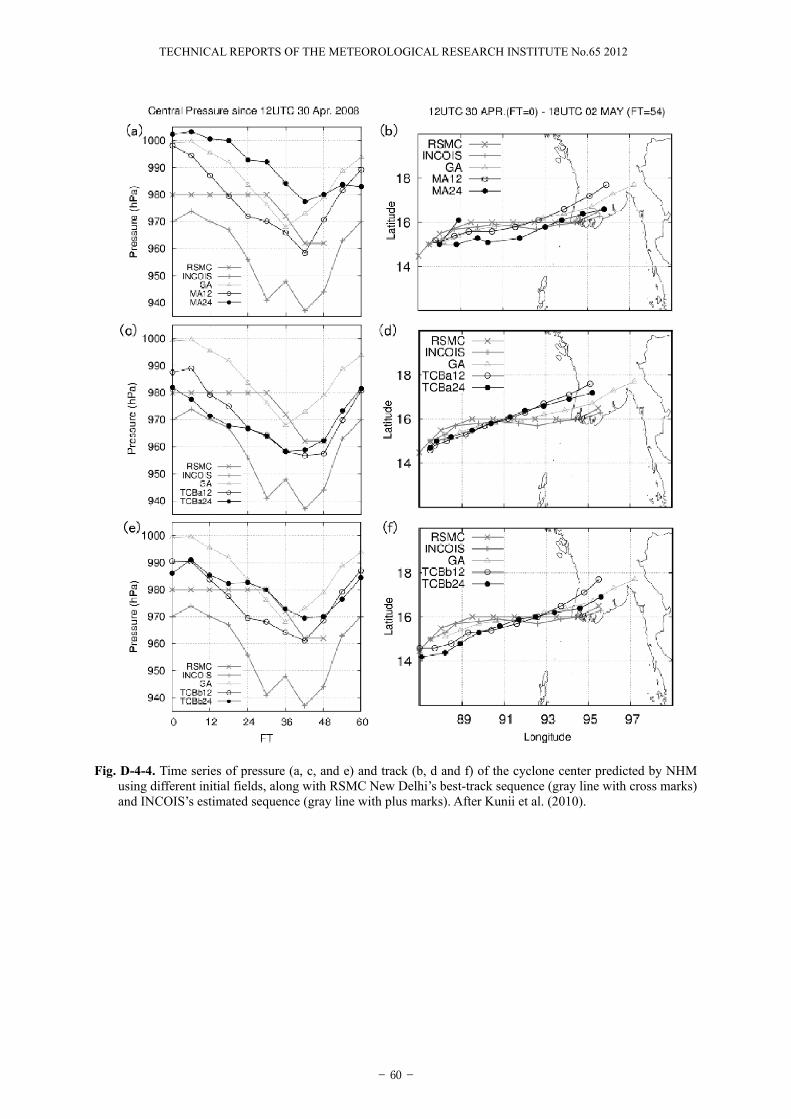
Figure D-4-4 presents time series of pressure (Figs. D-4-4a, D-4-4c, and D-4-4e) and track (Figs. D-4-4b, D-4-4d, and D-4-4f) of the cyclone center predicted by NHM using different initial conditions, along with the best track of RSMC New Delhi and the estimated sequence by the Indian National Centre for Ocean Information Services (INCOIS) (hereafter, collectively called “best tracks”).In the GA experiment, the center pressure became minimum (969hPa) at FT = 36 (0000 UTC 2 May). In best tracks, the center pressures reached minimum values at 0600 UTC 2 May. In this case, the simulated cyclone moved faster than best tracks and made landfall between 0000 and 0600 UTC 2 May at southern Myanmar. This earlier landfall could be the cause of the earlier occurrence of minimum pressure. In MA12, the cyclone central pressure at the initial time is almost the same as with the GA experiment. However, improvements in the prediction of cyclone intensity and speed are obtained. In this experiment, the timing of the minimum pressure is the same as in the INCOIS analysis, and the cyclone central pressure is consistently deeper than that in the GA experiment. Amelioration of dry bias at lower levels in analysis fields (Fig. D-4-3) may have helped the cyclone’s development.
Assimilation of TCB (TCBa12, TCBa24, TCBb12, and TCBb24) intensifies the cyclone. Cyclone central pressures at 1200 UTC 30 April (FT = 0) become deeper compared with experiments without TCB. Predicted cyclone center pressures at the mature stage in the TCBa experiments are between the RSMC New Delhi best track and the INCOIS estimation. The cyclones in the TCBb experiments tend to develop at a slower rate and to a lesser degree than in TCBa. A smaller gale-force wind radius in TCBb cyclones may have caused this difference. If we assume comparable reliabilities of the two cyclone intensity analyses, the center pressure predicted by TCBa24 seems best.
D-4-4. Summary We developed a mesoscale data assimilation system in low latitudes and conducted forecast
experiments for tropical cyclone Nargis. The JMA Meso 4D-Var system, which was designed for operational mesoscale data assimilation in the mid-latitudes, was modified for application to the tropics. In addition, a procedure for TCB calculation in the Bay of Bengal was developed based on the JMA’s operational scheme. At first, we statistically estimated the gale-force wind radius from the 10 min averaged maximum wind to make TCB profiles (TCBa) since no information about the gale-force
- 57 -

TECHNICAL REPORTS OF THE METEOROLOGICAL RESEARCH INSTITUTE No.65 2012
58
wind radius was available for Nargis. The results show that the DA system developed in this study is useful for the real-time simulation for TCs in Bay of Bengal. It is expected that in the future such a DA system will contribute to mitigating meteorological disasters in the low-latitude region, including Southeast Asia.
Table D-4-1. Specifications of the original Meso 4D-Var and this study. After Kunii et al. (2010).
- 58 -

TECHNICAL REPORTS OF THE METEOROLOGICAL RESEARCH INSTITUTE No.65 2012
58
wind radius was available for Nargis. The results show that the DA system developed in this study is useful for the real-time simulation for TCs in Bay of Bengal. It is expected that in the future such a DA system will contribute to mitigating meteorological disasters in the low-latitude region, including Southeast Asia.
Table D-4-1. Specifications of the original Meso 4D-Var and this study. After Kunii et al. (2010).
59
Fig. D-4-1. Domain of Meso 4D-Var in this study. After Kunii et al. (2010).
Fig. D-4-2. (a) Regression coefficients of geostrophic wind in mid-latitude. X- and Y-axis represent the model
vertical level and the regression coefficient. Here, rxx represents the regression coefficient for components between east-west and east-west, ryy represents that for components between north-south and north-south, rxy represents that for components between east-west and north-south, and ryx represents that for components between north-south and east-west (Ishikawa and Koizumi 2002a). (b) Weighting coefficients for the regression coefficients of geostrophic wind in mid-latitude. After Kunii et al. (2010).
(a) (b)
Fig. D-4-3. Vertical distributions of relative humidity averaged over the whole domain for the experiments of GA (dashed line with open triangle), MA12 (gray line with circle), and MA24 (black line with dot). After Kunii et al. (2010).
- 59 -
TECHNICAL REPORTS OF THE METEOROLOGICAL RESEARCH INSTITUTE No.65 2012
60
Fig. D-4-4. Time series of pressure (a, c, and e) and track (b, d and f) of the cyclone center predicted by NHM using different initial fields, along with RSMC New Delhi’s best-track sequence (gray line with cross marks) and INCOIS’s estimated sequence (gray line with plus marks). After Kunii et al. (2010).
- 60 -

TECHNICAL REPORTS OF THE METEOROLOGICAL RESEARCH INSTITUTE No.65 2012
60
Fig. D-4-4. Time series of pressure (a, c, and e) and track (b, d and f) of the cyclone center predicted by NHM using different initial fields, along with RSMC New Delhi’s best-track sequence (gray line with cross marks) and INCOIS’s estimated sequence (gray line with plus marks). After Kunii et al. (2010).
61
D-5. Near realtime retrieval of GNSS precipitable water vapor in low latitudes and mesoscale data assimilation experiment of Myanmar cyclone Nargis1 D-5-1. Abstract
A trial of near realtime (NRT) analysis of precipitable water vapor (PWV) using global ground based GPS (Global Positioning System) network was performed. Preliminary evaluation of the NRT retrieved GPS PWV in Singapore showed comparable accuracy with those obtained by posterior analyses that use IGS (International Global navigation satellite system Service) precise ephemeris.
Four-dimensional variational (4D-Var) data assimilation (DA) experiments using the NRT derived GPS PWV were conducted for the tropical cyclone (TC) Nargis in 2008. In order to analyze the initial field at 1200 UTC 30 April 2008, 12, 24, 36, and 48 h sequential DA experiments with 3 h assimilation windows were performed. The initial fields made by these DA experiments were applied to subsequent forecast experiments using a nonhydrostatic model (NHM) with a horizontal resolution of 10 km.
NHM predictions using initial fields produced by DA experiments that used only ordinary observational data (without GPS PWV) exhibited a large variation of predicted maximum TC intensity (958 to 983 hPa) for each experiment. In these experiments, a longer assimilation period did not necessarily result in better prediction. The DA of GPS PWV yielded a smaller variation of predicted maximum TC intensity (964 to 974 hPa), and a longer assimilation period tended to bring deeper depression of TC central pressure. Overall, with GPS data assimilated, the predicted TC intensities became closer to the best track data produced by the Regional Specialized Meteorological Centre (RSMC) New Delhi.
D-5-2. NRT analysis of PWV with global IGS stations Shoji (2009) introduced a procedure of NRT GPS analysis for the Japanese nationwide GPS
network named GEONET (GPS Earth Observation Network). In this study, the procedure proposed by Shoji (2009) was enhanced in order to enable NRT analysis for GPS stations not only in Japan but also all around the world.
In order to serve an operational numerical weather prediction (NWP), NRT GPS analysis refers to the retrieval of the PWV within several tens of minutes after the observation. The procedure of this study is based on the Precise Point Positioning (PPP) method (Zumberge et al. 1997). The PPP method enables us to analyze each GPS station independently with relatively low computational load. Therefore the method befits the NRT analysis of large number of GPS stations. However, the PPP requires precise value for orbits (positions and clock) of GPS satellites because the method treats satellite orbits as known parameter. Satellite orbit accuracy is crucial for PWV retrieval in the PPP method.
1 Y. Shoji, M. Kunii and K. Saito
- 61 -

TECHNICAL REPORTS OF THE METEOROLOGICAL RESEARCH INSTITUTE No.65 2012
62
Representative examples of GPS satellite orbits are provided by the IGS. Table D-5-1 summarizes the nominal accuracy of the IGS ephemerides. From the point of latency, IGU is only option for our NRT analysis. The nominal accuracy of an orbit in the IGU predicted part is about 5 cm. It is about twice as worse as those stored in IGF and IGR. On the other hand, the clock accuracy of the IGU predicted part is about 45 cm in length (about 70 mm in PWV). It is much worse than those stored in the IGF and the IGR. This suggests that correction to the clock offsets in the IGU predicted part is inevitable.
Table D-5-1. IGS Ephemerides as of January 2011.
Shoji (2009) selected an IGS station USUD which has been equipped with hydrogen maser atomic
clock, as a reference station to analyze the clock offsets of GPS satellites. This station was installed in July 1990, on the building roof of the Usuda Deep Space Center of the Japan Aerospace Exploration Agency (JAXA) in Saku city, Nagano Prefecture (red triangle in Fig. D-5-1 (a)). Firstly, the clock offset of USUD was analyzed by using the IGS rapid orbit (IGR), and then, the offset of USUD station clock was extrapolated for the next two days. Secondly, the offsets of GPS satellite clocks were analyzed while the extrapolated offsets of the USUD clock were kept fixed as a time reference. In this step, 23 GEONET stations (blue diamonds in Fig. D-5-1 (a)) were analyzed simultaneously while the satellites positions were kept fixed at orbits in IGU.
Fig. D-5-1. (a) Locations of GEONET GPS stations. Small dots: GEONET stations; large blue diamonds (◆):
GEONET station used for the analysis of satellite clock offsets in Shoji (2009); filled red triangle (▲): USUD IGS station. (b) Locations of IGS stations. Red diamonds (◆): IGS station used for the analysis of satellite clock offset in this study; green dots (●): hourly sites; blue dots (●): non hourly sites.
- 62 -

TECHNICAL REPORTS OF THE METEOROLOGICAL RESEARCH INSTITUTE No.65 2012
62
Representative examples of GPS satellite orbits are provided by the IGS. Table D-5-1 summarizes the nominal accuracy of the IGS ephemerides. From the point of latency, IGU is only option for our NRT analysis. The nominal accuracy of an orbit in the IGU predicted part is about 5 cm. It is about twice as worse as those stored in IGF and IGR. On the other hand, the clock accuracy of the IGU predicted part is about 45 cm in length (about 70 mm in PWV). It is much worse than those stored in the IGF and the IGR. This suggests that correction to the clock offsets in the IGU predicted part is inevitable.
Table D-5-1. IGS Ephemerides as of January 2011.
Shoji (2009) selected an IGS station USUD which has been equipped with hydrogen maser atomic
clock, as a reference station to analyze the clock offsets of GPS satellites. This station was installed in July 1990, on the building roof of the Usuda Deep Space Center of the Japan Aerospace Exploration Agency (JAXA) in Saku city, Nagano Prefecture (red triangle in Fig. D-5-1 (a)). Firstly, the clock offset of USUD was analyzed by using the IGS rapid orbit (IGR), and then, the offset of USUD station clock was extrapolated for the next two days. Secondly, the offsets of GPS satellite clocks were analyzed while the extrapolated offsets of the USUD clock were kept fixed as a time reference. In this step, 23 GEONET stations (blue diamonds in Fig. D-5-1 (a)) were analyzed simultaneously while the satellites positions were kept fixed at orbits in IGU.
Fig. D-5-1. (a) Locations of GEONET GPS stations. Small dots: GEONET stations; large blue diamonds (◆):
GEONET station used for the analysis of satellite clock offsets in Shoji (2009); filled red triangle (▲): USUD IGS station. (b) Locations of IGS stations. Red diamonds (◆): IGS station used for the analysis of satellite clock offset in this study; green dots (●): hourly sites; blue dots (●): non hourly sites.
63
The network which Shoji (2009) adopted for satellite clock correction (Fig. D-5-1 (a)) modifies satellite clock information around Japan. In order to correct crock information of all GPS satellites, IGS’s global GPS network was used as shown in Fig. D-5-1 (b).
Fig. D-5-2. (a) Two days PWV sequence at IGS site “NTUS” in Singapore from 27 to 28 July 2007. Gray dots (●): GPS PWVs obtained by using IGF; x marks: those by using IGU; lines: those by using corrected IGU in this study; red squares (□) radio-sonde in Singapore (48698). (b) Scatter diagram of PWV comparison between radio-sonde and GPS for 19 days in July 2007. Red squares (■); GPS PWVs obtained by using IGF; blue triangles (▲): those obtained by using corrected IGU in this study; gray x marks (×): those obtained by using IGU.
Figure D-5-2 shows the comparison of the PWV retrieved by GPS and radio-sonde in Singapore.
GPS PWVs obtained by using modified IGU (IGUm) in this study represent much the same performance with those obtained by using IGF. Those two agreed with radio-sonde observation with approximately 2 mm in root mean square (RMS) differences, whereas those obtained by using IGU resulted in large amount of errors (~21 mm in RMS).
D-5-3. Mesoscale data assimilation experiment of NRT GPS PWV for Myanmar cyclone Nargis
Kunii et al. (2010) modified the Meso 4D-Var in order to apply the system to low latitudes, and conducted DA experiments on Myanmar cyclone Nargis in 2008. Their results demonstrated the effectiveness of the DA system for the prediction of Nargis. They succeeded to reproduce the cyclone’s minimum central pressure lower than 960 hPa. Also, they suggested the significance of observation enhancement around the Bay of Bengal.
In order to assess the impact of GPS PWV for TC prediction in low latitudes, we conducted DA experiment using DA system developed by Kunii et al. (2010). We targeted 1200 UTC 30 April 2008 as the initial time for the NHM forecast experiments. It is about two days before landfall of Nargis in the Irrawaddy river delta around 1200 UTC 2 May.
The following initial conditions were tested. (a) GA:
- 63 -

TECHNICAL REPORTS OF THE METEOROLOGICAL RESEARCH INSTITUTE No.65 2012
64
JMA operational Global Analysis (GANAL) at 1200 UTC 30 April is used as the initial field. (b) MA12, 24, 36, and 48: Successive DA cycles with 3 h assimilation windows were performed. Assimilation periods of the
DA experiments were 12, 24, 36, and 48 h. Radio-sonde, synop (surface), ship, buoy, aircraft, wind and PWV fields retrieved from satellite-based microwave scatterometer/radiometer were assimilated with hourly data slots. GANAL at 1200 UTC 28 April was used as the initial condition for the first DA window and produced the first-guess field by the hydrostatic mesoscale spectral model of JMA (MSM) prediction. Fields analyzed by previous DA windows were used as initial conditions of subsequent DA windows.
(c) GPS12, 24, 36, and 48: These experiments are the same as the above MA experiments, except that GPS PWV is added to
the assimilation data during the entire assimilation period. Figure D-5-3 shows the domain of our DA and NWP experiments together with locations of assimilated GPS sites.
Figure D-5-4 plots the time series of TC central pressures predicted by NHM, along with RSMC
New Delhi’s best track and estimated sequence by the Indian National Centre for Ocean Information Services (INCOIS) (hereafter, labeled “best tracks” for descriptive purposes).
When GANAL at 1200 UTC 30 April was used as the initial field (GA), NHM predicted a minimum TC central pressure of 969 hPa at FT = 36. The 12 h DA of ordinary observational data (MA12) resulted in a deeper depression of 958 hPa at FT = 42. However, NHM predictions using initial fields produced by ordinary observational data (MA12, 24, 36, and 48) indicated a large variation of the minimum TC central pressures (958 to 983 hPa). Among these four experiments, 12 h data assimilation (MA12) produced the deepest pressure dip. The 24 h and 36 h DA resulted in a decrease of pressure depression of more than 10 hPa from MA12. Furthermore, MA48 had the poorest performance.
By assimilating GPS PWV (GPS12, 24, 36, and 48), the variation of predicted TC central pressures became smaller (964 to 974 hPa). GPS12 resulted in 6 hPa larger minimum pressure than that of
Fig. D-5-3. Locations of the 21 GPS stations used in this study. Black dots (•) denote IGS stations; open triangles (△) denote Sumatran GPS
Array (SuGAr); open diamonds (◇) denote GPS stations in the Andaman Islands. Station IDs expressed in four characters are placed near each station’s position. The ground surface altitude is expressed in shade. After Shoji et al. (2011).
- 64 -
TECHNICAL REPORTS OF THE METEOROLOGICAL RESEARCH INSTITUTE No.65 2012
64
JMA operational Global Analysis (GANAL) at 1200 UTC 30 April is used as the initial field. (b) MA12, 24, 36, and 48: Successive DA cycles with 3 h assimilation windows were performed. Assimilation periods of the
DA experiments were 12, 24, 36, and 48 h. Radio-sonde, synop (surface), ship, buoy, aircraft, wind and PWV fields retrieved from satellite-based microwave scatterometer/radiometer were assimilated with hourly data slots. GANAL at 1200 UTC 28 April was used as the initial condition for the first DA window and produced the first-guess field by the hydrostatic mesoscale spectral model of JMA (MSM) prediction. Fields analyzed by previous DA windows were used as initial conditions of subsequent DA windows.
(c) GPS12, 24, 36, and 48: These experiments are the same as the above MA experiments, except that GPS PWV is added to
the assimilation data during the entire assimilation period. Figure D-5-3 shows the domain of our DA and NWP experiments together with locations of assimilated GPS sites.
Figure D-5-4 plots the time series of TC central pressures predicted by NHM, along with RSMC
New Delhi’s best track and estimated sequence by the Indian National Centre for Ocean Information Services (INCOIS) (hereafter, labeled “best tracks” for descriptive purposes).
When GANAL at 1200 UTC 30 April was used as the initial field (GA), NHM predicted a minimum TC central pressure of 969 hPa at FT = 36. The 12 h DA of ordinary observational data (MA12) resulted in a deeper depression of 958 hPa at FT = 42. However, NHM predictions using initial fields produced by ordinary observational data (MA12, 24, 36, and 48) indicated a large variation of the minimum TC central pressures (958 to 983 hPa). Among these four experiments, 12 h data assimilation (MA12) produced the deepest pressure dip. The 24 h and 36 h DA resulted in a decrease of pressure depression of more than 10 hPa from MA12. Furthermore, MA48 had the poorest performance.
By assimilating GPS PWV (GPS12, 24, 36, and 48), the variation of predicted TC central pressures became smaller (964 to 974 hPa). GPS12 resulted in 6 hPa larger minimum pressure than that of
Fig. D-5-3. Locations of the 21 GPS stations used in this study. Black dots (•) denote IGS stations; open triangles (△) denote Sumatran GPS
Array (SuGAr); open diamonds (◇) denote GPS stations in the Andaman Islands. Station IDs expressed in four characters are placed near each station’s position. The ground surface altitude is expressed in shade. After Shoji et al. (2011).
65
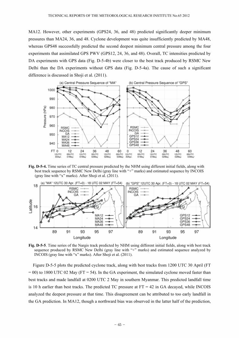
MA12. However, other experiments (GPS24, 36, and 48) predicted significantly deeper minimum pressures than MA24, 36, and 48. Cyclone development was quite insufficiently predicted by MA48, whereas GPS48 successfully predicted the second deepest minimum central pressure among the four experiments that assimilated GPS PWV (GPS12, 24, 36, and 48). Overall, TC intensities predicted by DA experiments with GPS data (Fig. D-5-4b) were closer to the best track produced by RSMC New Delhi than the DA experiments without GPS data (Fig. D-5-4a). The cause of such a significant difference is discussed in Shoji et al. (2011).
Fig. D-5-4. Time series of TC central pressure predicted by the NHM using different initial fields, along with best track sequence by RSMC New Delhi (gray line with “+” marks) and estimated sequence by INCOIS (gray line with “x” marks). After Shoji et al. (2011).
Fig. D-5-5. Time series of the Nargis track predicted by NHM using different initial fields, along with best track
sequence produced by RSMC New Delhi (gray line with “+” marks) and estimated sequence analyzed by INCOIS (gray line with “x” marks). After Shoji et al. (2011).
Figure D-5-5 plots the predicted cyclone track, along with best tracks from 1200 UTC 30 April (FT
= 00) to 1800 UTC 02 May (FT = 54). In the GA experiment, the simulated cyclone moved faster than best tracks and made landfall at 0200 UTC 2 May in southern Myanmar. This predicted landfall time is 10 h earlier than best tracks. The predicted TC pressure at FT = 42 in GA decayed, while INCOIS analyzed the deepest pressure at that time. This disagreement can be attributed to too early landfall in the GA prediction. In MA12, though a northward bias was observed in the latter half of the prediction,
- 65 -

TECHNICAL REPORTS OF THE METEOROLOGICAL RESEARCH INSTITUTE No.65 2012
66
moving speed and landfall time improved compared to GA. At FT = 42 in MA12, the predicted TC center was still located over the ocean, which might have led to further development of the TC at FT = 42.
MA24 exhibits a small southward bias in the first half of the prediction but decreases the bias in the latter half. As a result, the landfall location became closer to that of best tracks. Kunii et al. (2010) discussed the causes of these differences in the predicted TC track from the perspective of differences in steering flow.
No large differences in tracks between MA12 and GPS12, or between MA24 and GPS24, are apparent. GPS36 had a larger northward bias than MA36 from FT = 00 to FT = 36; after that, its moving direction changed to eastward. The predicted track of MA48 meandered largely north and south, even though the speed was slower than best tracks and landfall time was several hours delayed. GPS48 roughly followed the path of best tracks.
Overall, the large variation of predicted TC pressures and tracks represents the high sensitivity of TC prediction to the initial field and indicates the significance of precise analysis of the initial field. As pointed out by Kunii et al. (2010), poor observation density around the Bay of Bengal might cause the large variation in prediction results.
D-5-4. Summary Our results suggest the importance of accurate analysis around the TC center in the early stage.
Assimilation of GPS PWV improved prediction of intensity and track. However, the analyzed location of the TC center indicated a gap of several hundred kilometers from the best tracks. These facts indicate the necessity of further enhancing the observational network. Space-based Microwave radiometer and scatterometer data tend to be rejected around the TC center from DA in the quality check process. Novel approaches of quality control and/or direct assimilation of brightness temperatures may be needed in order to use more space-based remote sensing data. GPS observation is not affected by weather conditions; thus, it is always available as a continuous water vapor sensor. The results obtained in this study encourage the use of GPS, especially in data-sparse areas like the Bay of Bengal.
- 66 -

TECHNICAL REPORTS OF THE METEOROLOGICAL RESEARCH INSTITUTE No.65 2012
66
moving speed and landfall time improved compared to GA. At FT = 42 in MA12, the predicted TC center was still located over the ocean, which might have led to further development of the TC at FT = 42.
MA24 exhibits a small southward bias in the first half of the prediction but decreases the bias in the latter half. As a result, the landfall location became closer to that of best tracks. Kunii et al. (2010) discussed the causes of these differences in the predicted TC track from the perspective of differences in steering flow.
No large differences in tracks between MA12 and GPS12, or between MA24 and GPS24, are apparent. GPS36 had a larger northward bias than MA36 from FT = 00 to FT = 36; after that, its moving direction changed to eastward. The predicted track of MA48 meandered largely north and south, even though the speed was slower than best tracks and landfall time was several hours delayed. GPS48 roughly followed the path of best tracks.
Overall, the large variation of predicted TC pressures and tracks represents the high sensitivity of TC prediction to the initial field and indicates the significance of precise analysis of the initial field. As pointed out by Kunii et al. (2010), poor observation density around the Bay of Bengal might cause the large variation in prediction results.
D-5-4. Summary Our results suggest the importance of accurate analysis around the TC center in the early stage.
Assimilation of GPS PWV improved prediction of intensity and track. However, the analyzed location of the TC center indicated a gap of several hundred kilometers from the best tracks. These facts indicate the necessity of further enhancing the observational network. Space-based Microwave radiometer and scatterometer data tend to be rejected around the TC center from DA in the quality check process. Novel approaches of quality control and/or direct assimilation of brightness temperatures may be needed in order to use more space-based remote sensing data. GPS observation is not affected by weather conditions; thus, it is always available as a continuous water vapor sensor. The results obtained in this study encourage the use of GPS, especially in data-sparse areas like the Bay of Bengal.
67
D-6. Asymmetric features of near-surface wind fields in typhoons revealed by the JMA mesoscale analysis data1
Recently the relationships between azimuthal wavenumber-one inner-core structures of tropical cyclones
(TCs), and environmental vertical wind shear, have been increasingly investigated with numerical simulations
at high resolution and theoretical considerations. However, due to the lack of detailed observations, which are
usually obtained through a special field observational program, the results have not been endorsed by
observational studies in a systematic manner. A viable alternative for detailed observations is analytical gridded
data produced with a relatively high resolution by using a state-of-the-art data assimilation technique, such as
the mesoscale analysis (hereafter referred to as "meso-analysis") data operationally produced at the Japan
Meteorological Agency (JMA).
Over the years, researchers have developed parametric wind models to depict the surface winds within a TC.
Parametric models have shown utility in creating wind fields as input to models such as the wave model, storm
surge model, statistical-parametric model to predict TC wind radii, and pressure–wind model to relate the
minimum central pressure to maximum surface winds in TCs. In most of such studies storm motion is assumed
to be the only contributor to the near-surface wind asymmetry in TCs. Furthermore, most of previous
theoretical studies on the wind distribution in the TC boundary layer have focused on the effect of TC
translation on the wind distribution. Based on results from a real data simulation of Typhoon Chaba (2004),
however, Ueno (2008) suggested that vertical wind shear could play a dominant role in determining the wind
structure in the TC boundary layer insofar as the shear is significantly large. In the simulation low-level inflow
tends to occur in the downshear-left quadrant, in accordance with the preferred location of rainfall maximum,
and the strongest tangential wind is about 90
of azimuth downstream of the maximum inflow. A better
knowledge of the role of vertical wind shear in determining the near-surface wind asymmetry would help to
significantly improve parametric wind models.
The purpose of the present study is to document, in an extensive manner using the meso-analysis data, the
influence of environmental vertical wind shear on the wavenumber-one asymmetries of near-surface wind
components in the TC inner-core region. As a first step to quantify the shear contribution to the near-surface
wind asymmetry in real TCs, we analyze the wind fields at about 20 m height (the lowest analysis level)
obtained from the JMA operational meso-analysis, putting emphasis on the azimuthal location of wind
maximum and its relevance to shear and storm motion. For the purpose a total of 190 cases from 35 typhoons
observed during 2004–2007 seasons are examined. Figure D-6-1 shows the directional relationship between
shear and tangential wind maximum. The azimuth of tangential wind maximum is found by performing the
first-order Fourier decomposition of earth-relative wind field with respect to the surface center. In the figure
both the shear direction and azimuth of tangential wind maximum are defined relative to the direction of storm
1 M. Ueno and M. Kunii
- 67 -

TECHNICAL REPORTS OF THE METEOROLOGICAL RESEARCH INSTITUTE No.65 2012
68
motion. The storm motion vector is calculated from the JMA best-track position fixes. As expected, and in
accordance with various earlier observational studies, the wind maxima are found predominantly to the right of
TC motion. Interestingly, however, a small fraction (17 %) of the total cases exhibit a left-of-motion maximum
and it occurs only in cases in which the shear direction is nearly equal to the storm heading. This result is in
qualitative agreement with expectations from the simplified formulae derived in the study, which predict the
tangential wind maximum in storm-relative coordinates to the left of TC center facing in the direction of
enhanced eyewall convection (see Ueno and Kunii (2009) for more details).
Fig. D-6-1. Directional relationship between vertical wind shear and tangential wind maximum. Vertical axis denotes the direction (in degree) of shear relative to that of storm motion vector with positive (negative) values for the shear to the left (right) of the motion, while horizontal one represents the azimuthal direction (in degree) of tangential wind maximum relative to storm heading. The sampled cases are stratified into two groups according to whether the shear magnitude is greater than storm translation speed (closed triangles) or not (open circles). After Ueno and Kunii (2009).
- 68 -

TECHNICAL REPORTS OF THE METEOROLOGICAL RESEARCH INSTITUTE No.65 2012
68
motion. The storm motion vector is calculated from the JMA best-track position fixes. As expected, and in
accordance with various earlier observational studies, the wind maxima are found predominantly to the right of
TC motion. Interestingly, however, a small fraction (17 %) of the total cases exhibit a left-of-motion maximum
and it occurs only in cases in which the shear direction is nearly equal to the storm heading. This result is in
qualitative agreement with expectations from the simplified formulae derived in the study, which predict the
tangential wind maximum in storm-relative coordinates to the left of TC center facing in the direction of
enhanced eyewall convection (see Ueno and Kunii (2009) for more details).
Fig. D-6-1. Directional relationship between vertical wind shear and tangential wind maximum. Vertical axis denotes the direction (in degree) of shear relative to that of storm motion vector with positive (negative) values for the shear to the left (right) of the motion, while horizontal one represents the azimuthal direction (in degree) of tangential wind maximum relative to storm heading. The sampled cases are stratified into two groups according to whether the shear magnitude is greater than storm translation speed (closed triangles) or not (open circles). After Ueno and Kunii (2009).
69
D-7. Preliminary validation of TC structure function used in the JMA typhoon bogussing
procedure1
D-7-1. Introduction Tropical cyclone (TC) vortex initialization is one of the most crucial aspects of mesoscale TC
modeling (Chen 2008). The mesoscale models used for the prediction of TC intensity and/or wind and
rainfall distributions associated with TCs are required to be initialized with a realistic inner-core
structure. However the conventional observational network does not capture the detailed inner-core
structure. As a result, the initial vortex obtained by assimilating observational data is mostly weaker than
the observed one with a larger radius of maximum wind (RMW) (Ueno and Mashiko 2005; Braun et al.
2006). The lack of storm-scale details in the initial conditions likely prevents the model from producing
an accurate forecast of TC intensity due mainly to a vortex spinup problem (Elsberry 2002). Indeed, a
comparative numerical study conducted by Bender et al. (1993) has demonstrated that it is essential to
start with TC vortex of realistic intensity for accurate TC intensity forecasts.
At present, from an operational point of view, a feasible option to prepare a realistic TC inner-core
structure in the initial fields for high-resolution models such as JMA mesoscale model is to use the
so-called "TC bogus observations". At JMA, a typhoon bogussing procedure has been applied to model
initialization for TC forecasting. In the procedure, a climatological TC structure is constructed based on
real-time TC analysis at the RSMC (Regional Specialized Meteorological Center) Tokyo, and a set of
pseudo observations (or bogus observations) describing the TC structure are created around the TC
center and assimilated into the initial fields for the mesoscale model.
A noteworthy aspect of the JMA typhoon bogussing method is that the symmetric portion of the three
dimensional typhoon structures is totally determined by using an analytical TC structure function (Ueno
1989). The analytical function was originally developed to reproduce the climatological typhoon
structure obtained by Frank (1977) in the initial fields for an early version of the JMA global model.
Although the analytical function has been used since then to generate TC bogus observations, little
attention has been paid to the validity of its use in the current modeling environments, especially in the
high-resolution modeling ones. For example, detailed inner-core structures such as RMW are not always
correctly specified by the method since the wind fields of bogus typhoon are basically determined from
gale-force wind radius and central pressure through the analytical function. Furthermore, some key
parameters to determine the thermal structure of bogus typhoon is best tuned to the models with a
resolution of several tens of kilometers.
In the present study the possibility of improving the accuracy of structure function is explored using
mesoscale analysis data (Ueno and Kunii 2009), JTWC (Joint Typhoon Warning Center) best-track data,
and radiosonde observations for 2004–2007, as a first step toward appropriately applying the typhoon
bogussing method to high-resolution modeling framework.
1 M. Ueno
- 69 -

TECHNICAL REPORTS OF THE METEOROLOGICAL RESEARCH INSTITUTE No.65 2012
70
D-7-2. TC structure function In the typhoon bogussing procedure, an empirical radius parameter (hereafter referred to as RTY),
which demarcates a typhoon vortex from its environment, is determined at first from the gale-force wind
radius and the latitude of the storm center. RTY is defined as the radius at which the rotation speed
around the storm center of an air-ring initially located at the gale-force wind radius becomes zero as it
expands outward conserving absolute angular momentum. In most cases the values of RTY are within
the range of 300 to 1000 km. Once RTY is determined, then axisymmetric surface pressure profile is
specified by using an empirical formula (Fujita 1952) from the JMA real-time warning track
information regarding the central pressure and gale-force wind radius, and ambient surface pressure
(Ueno 1989). To avoid possible aliasing or wrong projection of near-core small-scale features onto the
large-scale ones, which could occur by imposing a tight eyewall on the model grid beyond its resolution,
the surface pressure profile is modified (or smoothed) in a somewhat arbitrary manner so as to fit the
model grid.
The D-value (deviation of axisymmetric geopotential height (
Z ) from ambient) at pressure
P can be
expressed as
D Z r ZB Rg
Td ln pPs
P
Rg
TBd ln pPB
P
Rg
T TB d ln pPs
P
Rg
TBd ln pPB
Ps
,
(D-7-1)
where the subscript
B denotes an azimuthal average (reference-value) at the RTY of the relevant
quantities.
r is radial distance from the storm's center and
R is the gas constant for dry air.
Ps is surface
pressure as a function of
r and
PB is the value of
Ps at the RTY. Remaining symbols are conventional.
The right-most first term is a measure of vertically integrated temperature deviation. On the other hand,
the second term indicates the D-value of
PB isobaric surface, which becomes increasingly negative
value with decreasing
Ps . Note here that the environmental fields, which need to calculate the
reference-values such as
TB , are taken from the most recent forecast (i.e., first guess for the analysis).
Then the problem is to determine the first term. To solve the problem it is assumed that the term can be
expressed by the following analytical function,
prZPpPpPp Tax
n
Tas ,lnlnexplnlnlnln 220
. (D-7-2)
The function includes some parameters that determine the warm core structure of the bogus typhoon.
The left-hand first term in Eq. (D-7-2) increases with height (or decreasing p) with a negative constant
. The second term is symmetric in the vertical about
p PTa0 in terms of
ln p and takes a maximum
value there for a positive integer
n .
Z decreases with increasing
(
0 ). The third term is
symmetric in the vertical about
p PTax in terms of
ln p and takes a maximum value there with the
peakedness determined by the parameter
(
0). By a combined effect of these three terms
Z takes
- 70 -

TECHNICAL REPORTS OF THE METEOROLOGICAL RESEARCH INSTITUTE No.65 2012
70
D-7-2. TC structure function In the typhoon bogussing procedure, an empirical radius parameter (hereafter referred to as RTY),
which demarcates a typhoon vortex from its environment, is determined at first from the gale-force wind
radius and the latitude of the storm center. RTY is defined as the radius at which the rotation speed
around the storm center of an air-ring initially located at the gale-force wind radius becomes zero as it
expands outward conserving absolute angular momentum. In most cases the values of RTY are within
the range of 300 to 1000 km. Once RTY is determined, then axisymmetric surface pressure profile is
specified by using an empirical formula (Fujita 1952) from the JMA real-time warning track
information regarding the central pressure and gale-force wind radius, and ambient surface pressure
(Ueno 1989). To avoid possible aliasing or wrong projection of near-core small-scale features onto the
large-scale ones, which could occur by imposing a tight eyewall on the model grid beyond its resolution,
the surface pressure profile is modified (or smoothed) in a somewhat arbitrary manner so as to fit the
model grid.
The D-value (deviation of axisymmetric geopotential height (
Z ) from ambient) at pressure
P can be
expressed as
D Z r ZB Rg
Td ln pPs
P
Rg
TBd ln pPB
P
Rg
T TB d ln pPs
P
Rg
TBd ln pPB
Ps
,
(D-7-1)
where the subscript
B denotes an azimuthal average (reference-value) at the RTY of the relevant
quantities.
r is radial distance from the storm's center and
R is the gas constant for dry air.
Ps is surface
pressure as a function of
r and
PB is the value of
Ps at the RTY. Remaining symbols are conventional.
The right-most first term is a measure of vertically integrated temperature deviation. On the other hand,
the second term indicates the D-value of
PB isobaric surface, which becomes increasingly negative
value with decreasing
Ps . Note here that the environmental fields, which need to calculate the
reference-values such as
TB , are taken from the most recent forecast (i.e., first guess for the analysis).
Then the problem is to determine the first term. To solve the problem it is assumed that the term can be
expressed by the following analytical function,
prZPpPpPp Tax
n
Tas ,lnlnexplnlnlnln 220
. (D-7-2)
The function includes some parameters that determine the warm core structure of the bogus typhoon.
The left-hand first term in Eq. (D-7-2) increases with height (or decreasing p) with a negative constant
. The second term is symmetric in the vertical about
p PTa0 in terms of
ln p and takes a maximum
value there for a positive integer
n .
Z decreases with increasing
(
0 ). The third term is
symmetric in the vertical about
p PTax in terms of
ln p and takes a maximum value there with the
peakedness determined by the parameter
(
0). By a combined effect of these three terms
Z takes
71
a maximum value at a pressure level between
p PTax and
p 0. The exact pressure level where
Z
is the largest depends on the relative contribution of the three subsidiary parameters,
,
and
.
The analytical function
Z was developed to reproduce the axisymmetric warm core structure of
typhoons presented in the Frank's composite study. The vertical profile of temperature anomaly for the
warm core is obtained by differentiating
Z with respect to
ln p. The key parameters included in the
function are
PTax and
PTa0 .
PTax denotes the pressure level where the maximum temperature anomaly
occurs. On the other hand,
PTa0 is considered to be the pressure level where the temperature anomaly
vanishes above the
PTax-level. Then the relationships between the key and subsidiary parameters are
easily obtained and can be represented as
00 lnlnlnln21
TaTaxTas PPPP , (D-7-3)
20
0022
0
lnln
lnln
lnlnlnlnlnln14
lnln
TaTax
Taxs
TasTaTaxTaxs
TaTax
PP
PP
PPPPPPn
nAA
PPn
, (D-7-4)
where
TaxsTaTaxTas PPPPPPA lnlnlnln2lnln 00 . (D-7-5)
Note here that both
and
could vary with radius because
Ps is a function of radius. As for
, its
calculation is done separately for the TC center and other places. If both
PTax and
PTa0 are prescribed
with
n 1, which is the current JMA operational setting, then
is the only parameter to be determined.
The value of
at the TC center can be obtained from Eq. (D-7-2) by giving D-value at a certain
pressure level. In the current operational setting, D-value at 700 hPa is used for this purpose since
geopotential height at 700 hPa can be estimated from the central pressure with acceptable accuracy
based on an empirical formula. If the resulting D-value at
p PTax is found positive, then
is modified
so as to make the D-value reduce to zero there. The value of
outside the center is obtained based on
the assumption that the temperature anomaly at
p PTa0 decreases linearly with radius and becomes
zero at the RTY. The assumption is reasonably consistent with Frank (1977) (see Figs. 3 and 4 therein)
and necessary for a smooth transition in thermal structure from bogus typhoon to environment at the
RTY.
The wind fields are derived from the geopotential height fields assuming the gradient wind balance
between mass and wind fields. In the boundary layer the gradient winds are modified to include the
surface friction. Asymmetric components of bogus typhoon are retrieved from the first guess fields and
added to the symmetric ones before the bogus observations are utilized in the data assimilation system
- 71 -

TECHNICAL REPORTS OF THE METEOROLOGICAL RESEARCH INSTITUTE No.65 2012
72
(Ueno 1995). In the current JMA data assimilation system, only wind bogus observations are
assimilated.
As mentioned above, the value of
at the TC center is derived from D-value at 700 hPa (algorithm
I) or D-value (
0) at
p PTax (algorithm II). Ueno (2000) revealed that in most cases
is determined
through algorithm II, suggesting the importance of the specified value of
PTax in determining the bogus
TC structure. Nevertheless,
PTax has long been used as a substitute for the pressure level (
PZa0) at which
D-value becomes zero, without sufficient validation of the setting.
D-7-3. Validation of TC structure The three-dimensional typhoon structure constructed using the TC structure function outlined in the
foregoing section may strongly depend on the previously specified surface pressure profile. In the
current bogussing procedure, the surface pressure profile is tailored to fit the model grid length to avoid
a kind of aliasing error. This modification usually results in a weaker cyclone with a larger RMW.
Figure D-7-1 compares the RMW of meso-analysis typhoon with that from the best-track data archived
by JTWC. The JTWC values of RMW are mostly confined to less than 100 km, while the meso-analysis
ones are distributed much more broadly extending up to 300 km. While this discrepancy might be
mostly attributable to the insufficient horizontal resolution of the data assimilation system, there is a
possibility that the use of Fujita's formula in the operational bogussing procedure, which determines the
axisymmetric component of sea-level pressure, is also responsible for the large RMW bias. The RMW
of bogus typhoon is basically determined through the formula from the following three parameters,
central and ambient sea-level pressures, and gale-force wind radius. This means that even if reliable
RMW value is available on a real-time basis, it cannot be directly used to modify the sea-level pressure
profile due to the limited degrees of freedom of the formula. The use of other formula such as that
proposed by Holland (2008) has the potential to overcome the disadvantage and generate improved
sea-level pressure profile including RMW.
Fig. D-7-1. Scatter diagram of JTWC best track (ordinate) versus meso-analysis (abscissa) for RMW (km). The total number of cases evaluated is 240.
- 72 -

TECHNICAL REPORTS OF THE METEOROLOGICAL RESEARCH INSTITUTE No.65 2012
72
(Ueno 1995). In the current JMA data assimilation system, only wind bogus observations are
assimilated.
As mentioned above, the value of
at the TC center is derived from D-value at 700 hPa (algorithm
I) or D-value (
0) at
p PTax (algorithm II). Ueno (2000) revealed that in most cases
is determined
through algorithm II, suggesting the importance of the specified value of
PTax in determining the bogus
TC structure. Nevertheless,
PTax has long been used as a substitute for the pressure level (
PZa0) at which
D-value becomes zero, without sufficient validation of the setting.
D-7-3. Validation of TC structure The three-dimensional typhoon structure constructed using the TC structure function outlined in the
foregoing section may strongly depend on the previously specified surface pressure profile. In the
current bogussing procedure, the surface pressure profile is tailored to fit the model grid length to avoid
a kind of aliasing error. This modification usually results in a weaker cyclone with a larger RMW.
Figure D-7-1 compares the RMW of meso-analysis typhoon with that from the best-track data archived
by JTWC. The JTWC values of RMW are mostly confined to less than 100 km, while the meso-analysis
ones are distributed much more broadly extending up to 300 km. While this discrepancy might be
mostly attributable to the insufficient horizontal resolution of the data assimilation system, there is a
possibility that the use of Fujita's formula in the operational bogussing procedure, which determines the
axisymmetric component of sea-level pressure, is also responsible for the large RMW bias. The RMW
of bogus typhoon is basically determined through the formula from the following three parameters,
central and ambient sea-level pressures, and gale-force wind radius. This means that even if reliable
RMW value is available on a real-time basis, it cannot be directly used to modify the sea-level pressure
profile due to the limited degrees of freedom of the formula. The use of other formula such as that
proposed by Holland (2008) has the potential to overcome the disadvantage and generate improved
sea-level pressure profile including RMW.
Fig. D-7-1. Scatter diagram of JTWC best track (ordinate) versus meso-analysis (abscissa) for RMW (km). The total number of cases evaluated is 240.
73
As described in the previous section, the thermal structure of bogus typhoon is primarily determined
by the two key parameters characterizing the warm-core structure,
PTax and
PTa0 . They respectively
indicate the pressure level that gives maximum temperature anomaly at the storm center, and the
pressure level where the temperature anomaly vanishes above the
PTax-level. Since the resultant warm
core structure of meso-analysis typhoons is built up from not only bogus observations, but also past and
current observations through the influence of the assimilating model, there is no assurance that the
parameters retrieved from meso-analysis typhoons coincide with those used in the bogussing procedure.
Figure D-7-2 plots the retrieved pressure levels. The retrieved
PTax tends to be significantly larger than
the value specified in the bogussing procedure (i.e., 250 hPa), especially for the cases with strong
environmental vertical wind shear. On the other hand, an overall shift to smaller values is found in the
retrieved
PTa0 , as compared to the specified value (i.e., 100 hPa). Note that the retrieved values could
change with the definition of environments (e.g., RTY).
As mentioned in the foregoing section, the pressure level (
PZa0) where the D-value becomes zero has
long been set to
PTax in the operational bogussing procedure possibly as a result of some early empirical
efforts to best tune the parameter to the numerical models of the time. Here in the present study the
validity of the
PZa0 setting is examined using the radiosonde and surface synoptic observations obtained
in the near-core region of typhoons during the period 2004–2007. The validation study is done using the
bogus observations that include asymmetric components extracted from the first guess fields. Table
D-7-1 shows the errors of bogus observations produced with the operational setting, comparing with
those with a trial parameter setting. The trial setting follows Ueno (2000) who found that the setting
PZa0 PTa0 leads to a smallest mean error irrespective of TC intensity when the fitting process to the
model grid is not applied to the surface pressure profile. Note that the fitting process usually results in
reducing the sharp pressure gradients near the center of an intense storm. So the parameters tuned with
the process being skipped are considered more appropriate for very high-resolution models. As seen in
Fig. D-7-2.
PTax (red square) and
PTa0 (blue triangle) retrieved from the meso-analysis typhoons. The vertical and horizontal axses indicate vertical level in pressure (hPa) and environmental vertical wind shear (m s-1), respectively. The total number of cases evaluated is 166.
- 73 -

TECHNICAL REPORTS OF THE METEOROLOGICAL RESEARCH INSTITUTE No.65 2012
74
the table, the trial set of parameters yields smaller errors throughout the depth of troposphere, consistent
with the verification results of Ueno (2000).
Table D-7-1. Root-mean-square (RMS) difference between bogus and radiosonde observations
evaluated for geopotential height (left three columns) and wind (right ones) within the radius obtained by multiplying the typhoon radius by factor 0.3. OPE and TRI denote the RMS differences obtained with an operational and a trial setting of key parameters, respectively. The numbers of cases evaluated are around 2000 for the surface and around 200 for the rest.
D-7-4. Summary In the present study, initial data problems arising with high-resolution TC modeling are discussed,
focusing on the validity of TC structure function used in the JMA bogussing procedure. It is found from
the study that (i) the radius of maximum wind (RMW) of the meso-analysis typhoons tends to be
significantly larger than that estimated by JTWC on the whole, (ii) the warm core structures of the
meso-analysis typhoons are significantly different from those intended by bogus observations, and (iii) a
modification of key parameters in the structure function could provide the inner-core TC structure more
consistent with radiosonde observations. These results suggest that there is still plenty room for
improvement in the current TC vortex initialization using the TC bogussing method, especially in the
context of high-resolution modeling.
- 74 -

TECHNICAL REPORTS OF THE METEOROLOGICAL RESEARCH INSTITUTE No.65 2012
74
the table, the trial set of parameters yields smaller errors throughout the depth of troposphere, consistent
with the verification results of Ueno (2000).
Table D-7-1. Root-mean-square (RMS) difference between bogus and radiosonde observations
evaluated for geopotential height (left three columns) and wind (right ones) within the radius obtained by multiplying the typhoon radius by factor 0.3. OPE and TRI denote the RMS differences obtained with an operational and a trial setting of key parameters, respectively. The numbers of cases evaluated are around 2000 for the surface and around 200 for the rest.
D-7-4. Summary In the present study, initial data problems arising with high-resolution TC modeling are discussed,
focusing on the validity of TC structure function used in the JMA bogussing procedure. It is found from
the study that (i) the radius of maximum wind (RMW) of the meso-analysis typhoons tends to be
significantly larger than that estimated by JTWC on the whole, (ii) the warm core structures of the
meso-analysis typhoons are significantly different from those intended by bogus observations, and (iii) a
modification of key parameters in the structure function could provide the inner-core TC structure more
consistent with radiosonde observations. These results suggest that there is still plenty room for
improvement in the current TC vortex initialization using the TC bogussing method, especially in the
context of high-resolution modeling.
75
D-8. Re-Analysis and re-forecast of Typhoon Vera (1959)1 D-8-1. Introduction Typhoon Vera attacked Japan around 18 JST (Japan Standard Time) on 26 September 1959. Vera caused the most tragic disasters after World War II, especially to the Ise Bay area located at middle part of the Japan Island, i.e. total amount of death toll was 5,098 and total number of total lost houses was 40,838. These were mainly induced by the storm surge, whose tide level at Nagoya port was 383 cm. The location of the Ise Bay and Nagoya To prevent such the tragic disaster, it is necessary that forecasts of its track and intensity are really precise. Japan Meteorological Agency (JMA) has started the long-term global-reanalysis project from 1958 to 2012, called as the JRA-55 (Ebita et al. 2009), which is a successor for the JRA-25 (Onogi et al. 2007). The JRA-55 project provided us the pilot analysis and observational data associated with Vera. In addition, we found the flight level and drop sonde observations by the US air force in the report for Vera of JMA (JMA 1961), and decided to use these observations in our study. The purposes of this study are a) the confirmation that the JMA operational meso scale analysis and forecast system are useful for super typhoon Vera, b) the challenge to assimilate the typhoon center pressure observations by direct observations.
D-8-2. Typhoon Vera Typhoon Vera was generated 200 km west of Eniwetok Atoll on 20 September 1959 as a tropical cyclone, developed to a typhoon at 15 JST on 23 September, and was recorded minimum pressure of 894 hPa (Fig. D-8-1, Fig. D-8-2). At the same time, the maximum wind speed of 70 m h-1 was estimated, and Vera became “super typhoon”. At 18 JST on 26 September, Vera made landfall on the Kii Peninsula and surface pressure of 929 hPa was recorded at the Shionomisaki observatory very near from the landfall point. This value is the second record as the surface pressure at landfall time in Japan. After the landfall, Vera passed the Japan Island within 6 h.
D-8-3. Methodology D-8-3-1. Observations, assimilation and forecast systems In this study, upper sounding, surface observation, ship, aircraft data were used (Fig. D-8-3). The aircraft observations are
1 T. Kawabata, M. Kunii, N. Kohno (JMA), K. Bessho, T. Nakazawa, Y. Honda (JMA) and K.Sawada
(JMA)
Fig. D-8-1. Best track of Typhoon Vera. Dates are indicated with UTC.
- 75 -

TECHNICAL REPORTS OF THE METEOROLOGICAL RESEARCH INSTITUTE No.65 2012
76
distributed in area of 20-30 N, 130-140 E. Aircraft data consists of flight level data by air-born sensor around 700 hPa height and drop sonde observations in the typhoon center and around the typhoon. An assimilation system in this study is the JMA operational meso scale nonhydrostatic 4-dimensional variational assimilation system (JNoVA; Honda et al. 2005). Horizontal resolutions of inner and our loop of JNoVA are 15 and 5 km, respectively. In JNoVA, an adjoint scheme of large scale condensation as moisture process is implemented. A forecast system is the JMA operational meso scale nonhydrostatic model (JMANHM; Saito et al. 2006). Its horizontal resolution is 5 km. A bulk cloud microphysics and the KF parameterization (Kain and Fritsch 1993) schemes are implemented.
D-8-3-2. Experimental design First, forecast using the JMA operational Global Spectrum Model (GSM) with 60 km grid spacing was conducted using JRA-55 analysis as initial conditions. Next, forecast using JMANHM with 20 km grid spacing was conducted, nested in the GSM result (hereafter NHM-20km) from 09 JST 25 September to 09 JST 26 Sep.. Finally, forecast using JMANHM with 5 km grid spacing was conducted, nested in NHM-20km from 03 JST 25 Sep. to 09 JST. This result was used as a first guess field. Assimilations using JNoVA were conducted from 09 JST 25 Sep. to 09 JST 26 Sep. with 3-h assimilation window. After that, 36-h forecast by JMANHM with
Fig. D-8-2. Time series of sea level pressure at the Typhoon Vera center. Assimilation term is shown in the horizontal line area and forecast term is shown in the shaded area.
Fig. D-8-3. Distribution of observational data in the 24-h assimilation term.. Surface (circles), ship (triangles), upper soundings (crosses), aircraft data at flight levels (squares), and drop sonde (stars).
- 76 -

TECHNICAL REPORTS OF THE METEOROLOGICAL RESEARCH INSTITUTE No.65 2012
76
distributed in area of 20-30 N, 130-140 E. Aircraft data consists of flight level data by air-born sensor around 700 hPa height and drop sonde observations in the typhoon center and around the typhoon. An assimilation system in this study is the JMA operational meso scale nonhydrostatic 4-dimensional variational assimilation system (JNoVA; Honda et al. 2005). Horizontal resolutions of inner and our loop of JNoVA are 15 and 5 km, respectively. In JNoVA, an adjoint scheme of large scale condensation as moisture process is implemented. A forecast system is the JMA operational meso scale nonhydrostatic model (JMANHM; Saito et al. 2006). Its horizontal resolution is 5 km. A bulk cloud microphysics and the KF parameterization (Kain and Fritsch 1993) schemes are implemented.
D-8-3-2. Experimental design First, forecast using the JMA operational Global Spectrum Model (GSM) with 60 km grid spacing was conducted using JRA-55 analysis as initial conditions. Next, forecast using JMANHM with 20 km grid spacing was conducted, nested in the GSM result (hereafter NHM-20km) from 09 JST 25 September to 09 JST 26 Sep.. Finally, forecast using JMANHM with 5 km grid spacing was conducted, nested in NHM-20km from 03 JST 25 Sep. to 09 JST. This result was used as a first guess field. Assimilations using JNoVA were conducted from 09 JST 25 Sep. to 09 JST 26 Sep. with 3-h assimilation window. After that, 36-h forecast by JMANHM with
Fig. D-8-2. Time series of sea level pressure at the Typhoon Vera center. Assimilation term is shown in the horizontal line area and forecast term is shown in the shaded area.
Fig. D-8-3. Distribution of observational data in the 24-h assimilation term.. Surface (circles), ship (triangles), upper soundings (crosses), aircraft data at flight levels (squares), and drop sonde (stars).
77
5 km grid spacing was conducted (NHM-5km) from 09 JST 26 Sep. to 21 JST 28 Sep.. Assimilation and forecast term associated with the Vera life time are indicated in Fig. D-8-2. Assimilation and forecast region is illustrated in Fig. D-8-4.
D-8-3-3. Assimilation method of drop sonde observations in the TC center In general, numerical models can not represent strong tropical cyclone (TC) similar with actual one, because of its coarse resolution and simplified physical processes. It is reasonable to suppose that observations in the TC center have bias error which is introduced by the model representativeness. In this study, since assimilation term was very short, the error was considered as random, that is, the error was treated as observational error, instead of bias. We gave the observational error using following method: When departure value (first guess – observation) is just 70 hPa, the value of observational error is set to 4.0 hPa which is five times of default value in JNoVA. When departure value is 10 hPa, the value is set to default value of 0.8 hPa (Eq. D-8-1). This specific value was determined under consideration of that a value of cost function when the observation in the TC center was assimilated became similar magnitude to that when not assimilated.
ERRobs = 0.8hPa ∗ �departure1�
+ 1�� if (departure > 10hPa). (D-8-1)
When the TC location in first guess field is far from the observational location, “twin cyclones” problem, which means that two cyclones, a bogus cyclone in the first guess field and an actual observed cyclone, exist in the analysis field may be induced. In our method, the problem hardly occurs, because the observational error becomes large under the situation, and the observation in the TC center is weekly assimilated. Our method could not correct the displacement error without other observations. Accordingly, our strategy is that typhoon is intensified by the assimilation of the TC center observation, and the displacement error is corrected by the other observations around the typhoon.
D-8-4. Results D-8-4-1. Drop sonde assimilation in the TC center In this section, effects of drop sonde assimilation in the TC center are discussed. Three observations were used in the assimilation term at 11 JST 25 Sep., 17 JST 25 Sep. 06 JST 26 Sep, respectively. Observations, analysis, first guess, and observational errors are illustrated in Fig. D-8-5. Since there are large departures (first guess – observation) in the first and second assimilation, observational errors are also set to large value. After several assimilations were conducted, departure became small at 06 JST 26 Sep.. Since observational error was set to small amount, the analysis of the center pressure and the location Fig. D-8-4. Model domain and orography
of JNoVA and NHM-5km. After Kawabata et al. (2011).
- 77 -

TECHNICAL REPORTS OF THE METEOROLOGICAL RESEARCH INSTITUTE No.65 2012
78
significantly closed to the observation.
D-8-4-2. Forecast results The TC center pressure and the position error in forecast result are compared with best track data (Fig. D-8-6). The value of center pressure at the initial time is 930 hPa, and difference between the forecast and observation is a small value of 10 hPa. The center pressure becomes large similarly to the observations during forecast time. Position error is also small less than 60 km during 12-h forecast. Forecast tracks around landfall time (Fig. D-8-7) is almost same with best track. Moving speed of forecast is slightly faster than that of observation, but difference is smaller than 1 h. Next, forecast results are compared with surface weather map. Surface pressure distribution in forecast results (middle panels in Fig. D-8-8) are very similar to the surface weather map (upper panels in Fig. D-8-8). The location and contour distribution of Vera, subtropical high pressure, cold and warm front are same. Especially, frontal rainfall distribution in the forecast result at 03 JST 27 Sep. are agreeing with frontal line
Fig. D-8-5. Surface pressure of first guess (thin black line), analysis results (thick black line) and observation (thick gray line). Observational errors (black dashed line) used in JNoVA are indicated with right axis. After Kawabata et al. (2011).
Fig. D-8-6. Forecast results of NHM-5km. Time sequence of center pressure of forecast result (thick line), best track (thin dashed line), and position error comparison with best track data (thin gray line) are indicated. Time sequence of position error uses right axis. After Kawabata et al. (2011).
Fig. D-8-7. Typhoon tracks of forecast result (solidline) and best track(dashed line) around thelandfall time. Largecircles indicate thelocations at 18 JST ineach track. AfterKawabata et al. (2011).
Ise Bay and
Nagoya port
- 78 -

TECHNICAL REPORTS OF THE METEOROLOGICAL RESEARCH INSTITUTE No.65 2012
78
significantly closed to the observation.
D-8-4-2. Forecast results The TC center pressure and the position error in forecast result are compared with best track data (Fig. D-8-6). The value of center pressure at the initial time is 930 hPa, and difference between the forecast and observation is a small value of 10 hPa. The center pressure becomes large similarly to the observations during forecast time. Position error is also small less than 60 km during 12-h forecast. Forecast tracks around landfall time (Fig. D-8-7) is almost same with best track. Moving speed of forecast is slightly faster than that of observation, but difference is smaller than 1 h. Next, forecast results are compared with surface weather map. Surface pressure distribution in forecast results (middle panels in Fig. D-8-8) are very similar to the surface weather map (upper panels in Fig. D-8-8). The location and contour distribution of Vera, subtropical high pressure, cold and warm front are same. Especially, frontal rainfall distribution in the forecast result at 03 JST 27 Sep. are agreeing with frontal line
Fig. D-8-5. Surface pressure of first guess (thin black line), analysis results (thick black line) and observation (thick gray line). Observational errors (black dashed line) used in JNoVA are indicated with right axis. After Kawabata et al. (2011).
Fig. D-8-6. Forecast results of NHM-5km. Time sequence of center pressure of forecast result (thick line), best track (thin dashed line), and position error comparison with best track data (thin gray line) are indicated. Time sequence of position error uses right axis. After Kawabata et al. (2011).
Fig. D-8-7. Typhoon tracks of forecast result (solidline) and best track(dashed line) around thelandfall time. Largecircles indicate thelocations at 18 JST ineach track. AfterKawabata et al. (2011).
Ise Bay and
Nagoya port
79
Fig. D-8-8. Upper panels are surface weather map, middle panels show surface pressure and 3-h accumulated rainfall amount, and bottoms are pseudo satellite images derived by forecast results. Blue lines in middle panels illustrate best tracks and reds illustrate forecast tracks.
(a) 09 JST 26 September (FT=00) (b) 03 JST 27 September (FT=18)
- 79 -

TECHNICAL REPORTS OF THE METEOROLOGICAL RESEARCH INSTITUTE No.65 2012
80
in the weather map. Weather distribution is estimated by pseudo satellite image (bottoms in Fig. D-8-8). These images are calculated through radiative transfer equations using model forecast results. Rainy or cloudy weather distributions in weather map are match to the estimated weather in the forecast results. Finally, time sequence of tide level in the forecast result is compared with the observation at Nagoya port in Fig. D-8-9. The tide level was calculated using Princeton Ocean Model (POM) with NHM-5km. The highest tide height of 389 cm in the observation is the maximum record in Japan. Correspondingly, forecast reproduced 352 cm height. Time sequence of forecast strongly resembles observation.
D-8-5. Conclusion Typhoon Vera made landfall Japan in 1959 and induced tragic disaster. Our motivations are confirmation of performance of JMA operational assimilation and forecast system for the typhoon, and challenge to assimilate directly the drop sonde observation in the TC center. We introduced the observational-error adjustment method, which the value of error is adjusted according to the departure value. This method provided the successful analysis of Vera. In the third assimilation, the departure became small, the analysis of the center pressure and the location significantly closed to the observation. In the forecast, time sequences of center pressure and location are very similar to best track data. Especially, track around landfall is almost same. Weather distribution in the forecast estimated by rainfall distribution and pseudo satellite image is comparable to the weather map. Finally, tide level calculated through POM is excellent compared with the observation. Super typhoon Vera before 50 years was well reanalyzed and re-forecasted using JNoVA and JMANHM. Direct assimilation of the drop sonde observation in the TC center was contributed to this result. The basic framework for meteorological disaster prevention was established after Vera and has been still valid. Our result can provide a realistic numerical 4-dimensional data and be useful for the validation on the framework.
Acknowledgement The authors are grateful to the U.S. army for their courageous observational work. The authors are thankful to the JRA-55 development team, the Climate Prediction Division of JMA, and the global
Fig. D-8-9. Time sequence of tide level of forecast (black line), observation (gray line with markers), and astronomical tide (gray dashed line).
- 80 -

TECHNICAL REPORTS OF THE METEOROLOGICAL RESEARCH INSTITUTE No.65 2012
80
in the weather map. Weather distribution is estimated by pseudo satellite image (bottoms in Fig. D-8-8). These images are calculated through radiative transfer equations using model forecast results. Rainy or cloudy weather distributions in weather map are match to the estimated weather in the forecast results. Finally, time sequence of tide level in the forecast result is compared with the observation at Nagoya port in Fig. D-8-9. The tide level was calculated using Princeton Ocean Model (POM) with NHM-5km. The highest tide height of 389 cm in the observation is the maximum record in Japan. Correspondingly, forecast reproduced 352 cm height. Time sequence of forecast strongly resembles observation.
D-8-5. Conclusion Typhoon Vera made landfall Japan in 1959 and induced tragic disaster. Our motivations are confirmation of performance of JMA operational assimilation and forecast system for the typhoon, and challenge to assimilate directly the drop sonde observation in the TC center. We introduced the observational-error adjustment method, which the value of error is adjusted according to the departure value. This method provided the successful analysis of Vera. In the third assimilation, the departure became small, the analysis of the center pressure and the location significantly closed to the observation. In the forecast, time sequences of center pressure and location are very similar to best track data. Especially, track around landfall is almost same. Weather distribution in the forecast estimated by rainfall distribution and pseudo satellite image is comparable to the weather map. Finally, tide level calculated through POM is excellent compared with the observation. Super typhoon Vera before 50 years was well reanalyzed and re-forecasted using JNoVA and JMANHM. Direct assimilation of the drop sonde observation in the TC center was contributed to this result. The basic framework for meteorological disaster prevention was established after Vera and has been still valid. Our result can provide a realistic numerical 4-dimensional data and be useful for the validation on the framework.
Acknowledgement The authors are grateful to the U.S. army for their courageous observational work. The authors are thankful to the JRA-55 development team, the Climate Prediction Division of JMA, and the global
Fig. D-8-9. Time sequence of tide level of forecast (black line), observation (gray line with markers), and astronomical tide (gray dashed line).
81
model team of the ReVera project, especially, Dr. H. Kamahori, Mr. A. Ebita and Mr. Y. Ohta, Mr. Shindo. They provided us pilot data, observation data, and the forecast result of GSM. This study was partly supported by the Japanese Ministry of Education, Culture, Sports, Science and Technology (MEXT) through a Grant-in-Aid for Scientific Research (21244074) "Study of advanced data assimilation and cloud resolving ensemble technique for prediction of local heavy rainfall".
- 81 -

TECHNICAL REPORTS OF THE METEOROLOGICAL RESEARCH INSTITUTE No.65 2012
82
D-9. Development of Air-Sea Bulk Transfer Coefficients and Roughness Length in JMA Non-Hydrostatic Model1
D-9-1. IntroductionNew formulation of air-sea bulk transfer coefficients and roughness lengths are introduced in
JMA-NHM (Saito et al. 2006) to improve the representation of exchange of momentum, sensible and latent heat flux over the ocean surface applied to intense tropical cyclone (TC) (Wong et al. 2010).Prediction of TC movement using numerical weather prediction (NWP) model has improved in recentdecades due to the advance made in model dynamics and physical processes, data assimilation methods and ensemble prediction system to facilitate the disaster preparedness and mitigation. In addition, TC intensity and wind distribution are inevitably important to assess the impact of high winds and vulnerable areas of wind destruction. More accurate prediction requires development of key physical processes, such as air-sea interaction, to simulate realistic structure and evolution of TC in NWP model. For instance in Powell et al. (2003) and Donelan et al. (2004), the drag coefficient of momentum or surface momentum flux are found to level off as wind speeds increase above hurricane force. Results from other field experiments (Belamari 2005) also suggest similar saturation properties of bulk coefficients in high wind regime. The existing drag coefficient formulation adopted in operational NWP models, for example in JMA-NHM, based on extrapolation of results from past field studies of surface momentum flux measurement under low and moderate wind speed situations, is therefore likely to be inadequate when applied to intense TC and extreme wind conditions. In the present work, the new bulk transfer coefficients and roughness lengths are implemented in NHM to study an intense TC affecting the South China Sea. Positive impacts are found on the forecasts of TC intensity, wind structure and precipitation pattern.
According to the bulk formulation of aerodynamics, the momentum flux, heat flux and moisture flux are expressed as follows,
( )( )qqUCquqw
UCuw
UCuuw
sq
sh
m
−==−
−==−
==−
**''
**''
22*
''
θθθθ
where Cm, Ch, Cq are respectively bulk transfer coefficients for momentum, heat and moisture, |U| the mean horizontal wind speed at 10 m above surface. In the original scheme of bulk transfer coefficients in JMA-NHM based on Kondo (1975) and Beljaars (1995), the coefficients vary linearly with the wind speed larger than moderate wind strength (~15 ms-1). A saturation behaviour of Cm for wind speeds exceeding 30 ms-1 is introduced as a new formulation of surface momentum flux in NHM following Powell et al. (2003) and Donelan et al. (2004). Similar level-off in Ch and Cq (Lebeaupin et al. 2007)are implemented in the new scheme. Fig. D-9-1(a) shows the variation of the bulk transfer coefficients in the new scheme against wind speeds at 10 m under neutral condition. In order to consider effects of wave parameters like wave height and periods, modifications of roughness length according to Taylor and Yelland (2001) and Oost et al. (2002) are implemented in the roughness lengths of momentum
1 W.K. Wong, S. Sumdin (TMD) and S.T. Lai (HKO)
- 82 -
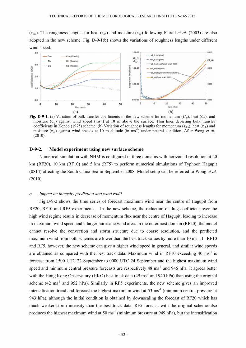
TECHNICAL REPORTS OF THE METEOROLOGICAL RESEARCH INSTITUTE No.65 2012
82
D-9. Development of Air-Sea Bulk Transfer Coefficients and Roughness Length in JMA Non-Hydrostatic Model1
D-9-1. IntroductionNew formulation of air-sea bulk transfer coefficients and roughness lengths are introduced in
JMA-NHM (Saito et al. 2006) to improve the representation of exchange of momentum, sensible and latent heat flux over the ocean surface applied to intense tropical cyclone (TC) (Wong et al. 2010).Prediction of TC movement using numerical weather prediction (NWP) model has improved in recentdecades due to the advance made in model dynamics and physical processes, data assimilation methods and ensemble prediction system to facilitate the disaster preparedness and mitigation. In addition, TC intensity and wind distribution are inevitably important to assess the impact of high winds and vulnerable areas of wind destruction. More accurate prediction requires development of key physical processes, such as air-sea interaction, to simulate realistic structure and evolution of TC in NWP model. For instance in Powell et al. (2003) and Donelan et al. (2004), the drag coefficient of momentum or surface momentum flux are found to level off as wind speeds increase above hurricane force. Results from other field experiments (Belamari 2005) also suggest similar saturation properties of bulk coefficients in high wind regime. The existing drag coefficient formulation adopted in operational NWP models, for example in JMA-NHM, based on extrapolation of results from past field studies of surface momentum flux measurement under low and moderate wind speed situations, is therefore likely to be inadequate when applied to intense TC and extreme wind conditions. In the present work, the new bulk transfer coefficients and roughness lengths are implemented in NHM to study an intense TC affecting the South China Sea. Positive impacts are found on the forecasts of TC intensity, wind structure and precipitation pattern.
According to the bulk formulation of aerodynamics, the momentum flux, heat flux and moisture flux are expressed as follows,
( )( )qqUCquqw
UCuw
UCuuw
sq
sh
m
−==−
−==−
==−
**''
**''
22*
''
θθθθ
where Cm, Ch, Cq are respectively bulk transfer coefficients for momentum, heat and moisture, |U| the mean horizontal wind speed at 10 m above surface. In the original scheme of bulk transfer coefficients in JMA-NHM based on Kondo (1975) and Beljaars (1995), the coefficients vary linearly with the wind speed larger than moderate wind strength (~15 ms-1). A saturation behaviour of Cm for wind speeds exceeding 30 ms-1 is introduced as a new formulation of surface momentum flux in NHM following Powell et al. (2003) and Donelan et al. (2004). Similar level-off in Ch and Cq (Lebeaupin et al. 2007)are implemented in the new scheme. Fig. D-9-1(a) shows the variation of the bulk transfer coefficients in the new scheme against wind speeds at 10 m under neutral condition. In order to consider effects of wave parameters like wave height and periods, modifications of roughness length according to Taylor and Yelland (2001) and Oost et al. (2002) are implemented in the roughness lengths of momentum
1 W.K. Wong, S. Sumdin (TMD) and S.T. Lai (HKO)
83
(zom). The roughness lengths for heat (zoh) and moisture (zoq) following Fairall et al. (2003) are also adopted in the new scheme. Fig. D-9-1(b) shows the variations of roughness lengths under different wind speed.
(a) (b)Fig. D-9-1. (a) Variation of bulk transfer coefficients in the new scheme for momentum (Cm), heat (Ch), and
moisture (Cq) against wind speed (ms-1) at 10 m above the surface. Thin lines depicting bulk transfer coefficients in Kondo (1975) scheme. (b) Variation of roughness lengths for momentum (z0m), heat (z0h) and moisture (z0q) against wind speeds at 10 m altitude (in ms-1) under neutral condition. After Wong et al.(2010).
D-9-2. Model experiment using new surface schemeNumerical simulation with NHM is configured in three domains with horizontal resolution at 20
km (RF20), 10 km (RF10) and 5 km (RF5) to perform numerical simulations of Typhoon Hagupit (0814) affecting the South China Sea in September 2008. Model setup can be referred to Wong et al.(2010).
a. Impact on intensity prediction and wind radiiFig.D-9-2 shows the time series of forecast maximum wind near the centre of Hagupit from
RF20, RF10 and RF5 experiments. In the new scheme, the reduction of drag coefficient over the high wind regime results in decrease of momentum flux near the centre of Hagupit, leading to increase in maximum wind speed and a larger hurricane wind area. In the outermost domain (RF20), the model cannot resolve the convection and storm structure due to coarse resolution, and the predicted maximum wind from both schemes are lower than the best track values by more than 10 ms-1. In RF10 and RF5, however, the new scheme can give a higher wind speed in general, and similar wind speeds are obtained as compared with the best track data. Maximum wind in RF10 exceeding 40 ms-1 is forecast from 1500 UTC 22 September to 0000 UTC 24 September and the highest maximum wind speed and minimum central pressure forecasts are respectively 48 ms-1 and 946 hPa. It agrees better with the Hong Kong Observatory (HKO) best track data (49 ms-1 and 940 hPa) than using the original scheme (42 ms-1 and 952 hPa). Similarly in RF5 experiments, the new scheme gives an improved intensification trend and forecast the highest maximum wind at 53 ms-1 (minimum central pressure at 943 hPa), although the initial condition is obtained by downscaling the forecast of RF20 which has much weaker storm intensity than the best track data. RF5 forecast with the original scheme also produces the highest maximum wind at 50 ms-1 (minimum pressure at 949 hPa), but the intensification
84
trend is slower than that from the new scheme. Therefore, the improved forecasts of maximum wind speed and central pressure for Hagupit suggest that the new scheme works effectively to enhance the intensity of strong tropical cyclone in NHM with horizontal grid resolution of 10 km or above.
In wind distribution forecasts, both RF10 experiments using original and new schemes (Fig.D-9-4a and Fig.D-9-4b) can predict areas of hurricane force wind. Moreover, a comma shape annular pattern of distribution is reproduced using the new scheme. Hurricane wind radii are about one degree over the northwestern, northeastern and southeastern quadrants while a smaller radius is forecast to the southwest. This compares favourably with the wind distribution from the NOAA Multi-Platform Satellite Wind (MPSW) Analysis (Knaff and DeMaria, 2006) (Fig.D-9-3), with hurricane wind radii (red shade) ranged from 100 to 140 km over the four quadrants. Fig.D-9-4c and Fig.D-9-4d show the wind distribution forecasts from RF5 experiments. Annular region of hurricane wind area is also forecast by the original scheme, but the area over northwest quadrant is smaller than both the new scheme and the MPSW analysis.
Fig. D-9-2. Time series of maximum wind near the centre of Hagupit from RF20, RF10 and RF5 using the original (dashed line) and new schemes (solid line). Maximum winds from HKO best track analysis are given in black dots. After Wong et al. (2010).
Fig. D-9-3. Surface wind distribution at 1200 UTC 23 September by NOAA Multi Platform Satellite Wind Analysis. After Wong et al. (2010).
(a) RF10 (original scheme) (b) RF10 (new scheme) (c) RF5 (original scheme) (d) RF5 (new scheme)Fig. D-9-4. Forecasts of surface wind barbs and isotach at 1400 UTC 23 September 2008 using the (a) original and (b)
new schemes in RF10 experiments. The color shading of green / blue / red / violet / yellow represents areas of fresh(8.0-10.7 ms-1) / strong / gale / storm / hurricane force winds respectively. (c)-(d) Similar forecasts from RF5 experiments. Area in Fig.D-9-4 is shown by dashed line boxes. After Wong et al. (2010).
b. Effects in precipitation forecast Heat and moisture fluxes are enhanced due to larger heat and moisture bulk coefficients in the
- 83 -

TECHNICAL REPORTS OF THE METEOROLOGICAL RESEARCH INSTITUTE No.65 2012
84
trend is slower than that from the new scheme. Therefore, the improved forecasts of maximum wind speed and central pressure for Hagupit suggest that the new scheme works effectively to enhance the intensity of strong tropical cyclone in NHM with horizontal grid resolution of 10 km or above.
In wind distribution forecasts, both RF10 experiments using original and new schemes (Fig.D-9-4a and Fig.D-9-4b) can predict areas of hurricane force wind. Moreover, a comma shape annular pattern of distribution is reproduced using the new scheme. Hurricane wind radii are about one degree over the northwestern, northeastern and southeastern quadrants while a smaller radius is forecast to the southwest. This compares favourably with the wind distribution from the NOAA Multi-Platform Satellite Wind (MPSW) Analysis (Knaff and DeMaria, 2006) (Fig.D-9-3), with hurricane wind radii (red shade) ranged from 100 to 140 km over the four quadrants. Fig.D-9-4c and Fig.D-9-4d show the wind distribution forecasts from RF5 experiments. Annular region of hurricane wind area is also forecast by the original scheme, but the area over northwest quadrant is smaller than both the new scheme and the MPSW analysis.
Fig. D-9-2. Time series of maximum wind near the centre of Hagupit from RF20, RF10 and RF5 using the original (dashed line) and new schemes (solid line). Maximum winds from HKO best track analysis are given in black dots. After Wong et al. (2010).
Fig. D-9-3. Surface wind distribution at 1200 UTC 23 September by NOAA Multi Platform Satellite Wind Analysis. After Wong et al. (2010).
(a) RF10 (original scheme) (b) RF10 (new scheme) (c) RF5 (original scheme) (d) RF5 (new scheme)Fig. D-9-4. Forecasts of surface wind barbs and isotach at 1400 UTC 23 September 2008 using the (a) original and (b)
new schemes in RF10 experiments. The color shading of green / blue / red / violet / yellow represents areas of fresh(8.0-10.7 ms-1) / strong / gale / storm / hurricane force winds respectively. (c)-(d) Similar forecasts from RF5 experiments. Area in Fig.D-9-4 is shown by dashed line boxes. After Wong et al. (2010).
b. Effects in precipitation forecast Heat and moisture fluxes are enhanced due to larger heat and moisture bulk coefficients in the
- 84 -

TECHNICAL REPORTS OF THE METEOROLOGICAL RESEARCH INSTITUTE No.65 2012
84
trend is slower than that from the new scheme. Therefore, the improved forecasts of maximum wind speed and central pressure for Hagupit suggest that the new scheme works effectively to enhance the intensity of strong tropical cyclone in NHM with horizontal grid resolution of 10 km or above.
In wind distribution forecasts, both RF10 experiments using original and new schemes (Fig.D-9-4a and Fig.D-9-4b) can predict areas of hurricane force wind. Moreover, a comma shape annular pattern of distribution is reproduced using the new scheme. Hurricane wind radii are about one degree over the northwestern, northeastern and southeastern quadrants while a smaller radius is forecast to the southwest. This compares favourably with the wind distribution from the NOAA Multi-Platform Satellite Wind (MPSW) Analysis (Knaff and DeMaria, 2006) (Fig.D-9-3), with hurricane wind radii (red shade) ranged from 100 to 140 km over the four quadrants. Fig.D-9-4c and Fig.D-9-4d show the wind distribution forecasts from RF5 experiments. Annular region of hurricane wind area is also forecast by the original scheme, but the area over northwest quadrant is smaller than both the new scheme and the MPSW analysis.
Fig. D-9-2. Time series of maximum wind near the centre of Hagupit from RF20, RF10 and RF5 using the original (dashed line) and new schemes (solid line). Maximum winds from HKO best track analysis are given in black dots. After Wong et al. (2010).
Fig. D-9-3. Surface wind distribution at 1200 UTC 23 September by NOAA Multi Platform Satellite Wind Analysis. After Wong et al. (2010).
(a) RF10 (original scheme) (b) RF10 (new scheme) (c) RF5 (original scheme) (d) RF5 (new scheme)Fig. D-9-4. Forecasts of surface wind barbs and isotach at 1400 UTC 23 September 2008 using the (a) original and (b)
new schemes in RF10 experiments. The color shading of green / blue / red / violet / yellow represents areas of fresh(8.0-10.7 ms-1) / strong / gale / storm / hurricane force winds respectively. (c)-(d) Similar forecasts from RF5 experiments. Area in Fig.D-9-4 is shown by dashed line boxes. After Wong et al. (2010).
b. Effects in precipitation forecast Heat and moisture fluxes are enhanced due to larger heat and moisture bulk coefficients in the
85
new scheme, resulting in enhancement of vertical eddy transport of moisture and heat to sustain the development of Hagupit, as well as an increase of moisture in cloud and convective parameterization processes of NHM. Fig. D-9-5 (a)-(c) show the forecasts of sea level pressure and 1-hour accumulated rainfall at 1400 UTC 23 September 2008 from RF20, RF10 and RF5 using the original (top panel) and new scheme (bottom panel). Using the new scheme, spiral rainbands are better predicted when compared to radar reflectivity and TRMM rainfall rate. Improvements in the model forecast on the intensity and structure of rainbands are useful for nowcasting application and very-short-range forecast of the heavy precipitation due to passage of intense tropical cyclones (Lai and Wong 2006).
(d)
(a) RF20 (b) RF10 (c) RF5 (e)Fig. D-9-5. Forecast mean-sea-level pressure (contour) and 1-hr accumulated rainfall (color shade) by (a) RF20, (b) RF10
and (c) RF5 at 14 UTC 23 September 2008 using the original scheme (top panel) and new scheme (bottom panel);(d) Rainfall rate estimate at 1425 UTC from TRMM (2A12 product from JAXA/EORC Tropical Cyclone Database);(e) Plan position indicator (PPI) display of radar reflectivity at 1405 UTC. After Wong et al. (2010).
D-9-3. Summary and Future DevelopmentUsing the new scheme of air-sea bulk transfer coefficients and roughness lengths in JMA-NHM,
an increase in forecast maximum wind speed with a lower central pressure of Typhoon Hagupit are obtained, due to reduced drag coefficient and larger heat and moisture bulk coefficients in high wind regime. They contribute positively to the exchange of surface fluxes to sustain the development of Hagupit, distribution of high wind areas and rainbands near the centre of Hagupit. The new scheme thus provides potential benefits in using NHM to simulate other intense tropical cyclones and effects of bulk coefficients in high wind regime for weather forecasts and climate studies on wind-pressurerelationship of intense tropical cyclones. The roughness lengths are modified and sea-wave effect is considered in the new scheme, though more accurate specification of wave parameter values requires future in-depth study using coupled atmosphere-wave model or field experiments.
- 85 -