Mario Ragwitz, Arne Klein, Anne Held Fraunhofer Institute Systems and Innovation Research (Fh-ISI)


D. Möst / W. Fichtner / M. Ragwitz / D. Veit (eds.)
New methods for energy market modelling Proceedings of the First European Workshop on Energy Market Modellingusing Agent-Based Computational Economics


New methods forenergy market modelling
Proceedings of the First European Workshopon Energy Market Modelling using Agent-BasedComputational Economics
1st EMMACE Workshop2007, 26th OctoberKarlsruhe, Germany
D. MöstW. FichtnerM. RagwitzD. Veit(eds.)

Impressum
Universitätsverlag Karlsruhec/o UniversitätsbibliothekStraße am Forum 2D-76131 Karlsruhewww.uvka.de
Dieses Werk ist unter folgender Creative Commons-Lizenz lizenziert: http://creativecommons.org/licenses/by-nc-nd/2.0/de/
Universitätsverlag Karlsruhe 2008 Print on Demand
ISBN: 978-3-86644-238-2

Preface Stakeholders in the electricity sector in many countries are facing challenges
due to market liberalisation, climate policy and the promotion of renewable energy
sources. The interaction between markets and environmental policy instruments is
an issue of increasing importance. A promising approach for the scientific analysis
of these developments is the field of agent-based simulation. Agent-based compu-
tational economics is a relatively young research paradigm that offers methods for
simulating energy markets. A growing number of researchers have developed
agent-based models to simulate the development of energy markets in the light of
the above mentioned challenges.
The inspiration for organizing the first European workshop on Energy Market
Modelling using Agent-Based Computational Economics (1. EMMACE work-
shop) came from the PowerACE project (www.powerace.com). In this project, the
following project partners carried out an agent-based simulation of the German
power market:
- the Fraunhofer Institute for Systems and Innovation Research (ISI) in
Karlsruhe (Competence Center Energy Policy and Energy Systems),
- the Chair of E-Business and E-Government, University of Mannheim, and
- the Institute for Industrial Production (IIP), working group “energy system
analysis and environment”, Universität Karlsruhe (TH).
As an associated partner the Chair of Energy Economics, Brandenburg Univer-
sity of Technology Cottbus was involved in the project.
Within the project it became evident that agent-based simulation models were
becoming increasingly popular amongst electricity market modellers. This devel-
opment can be explained by the additional opportunities this modelling paradigm
provides for the analysis of economic systems when compared to more traditional
equilibrium or optimisation models. Aspects like learning effects in repeated in-
teractions, asymmetric information, imperfect competition, or strategic interaction
and collusion can be included in a more realistic way in agent-based models.
As the field of energy market modelling with agent-based computational eco-
nomics is very heterogeneous, the objective of the workshop was to bring together
the different modellers and to learn about the potential of this valuable modelling
approach in different fields of the energy market.

This book contains a compilation of several papers and research projects in the
field of energy market modelling using agent-based computational economics
which were presented at the first EMMACE-workshop.
As the organizers of the workshop and editors of these proceedings, we were
delighted with the good attendance, which is reflected in the internationality and
interdisciplinarity of the participants and the scope of the contributed papers. We
are pleased to be able to make a contribution, which may foster the exchange of
scientific approaches and their practical application in the field of agent-based
computational economics. We would like to thank all the authors and the partici-
pants of the workshop.
It is a pleasant duty to express our sincere gratitude to the Excellence Initiative
of the German Research Foundation (DFG), which financed the Young Investiga-
tor Group (YIG) of Dr. D. Möst and the first EMMACE-workshop. Furthermore,
we are grateful to the VolkswagenStiftung and especially Professor Hagen Hof,
who financed the PowerACE-project. Without the financial support provided by
the VolkswagenStiftung in their programme for funding researchers in the inter-
disciplinary field of environmental research, such an interdisciplinary and vision-
ary project would not have been possible.
Karlsruhe, March 2008
The editors

1
Table of contents
Agent-based Modeling of Oligopolistic Competition in the
German Electricity Market 3
Anke Weidlich, Daniel Veit Chair of Business Administration and Information Systems
E-Business and E-Government - University of Mannheim
The hungarian electrical energy sector - an agent based model 15
Scabolcs Szekeres
Joint Research Centre - Institute for Prospective Technological Studies, Sevilla
Impact of emission allocation schemes on
power plant investments 29
Massimo Genoese, Dominik Möst, Philip Gardyan, Otto Rentz
Institute for Industrial Production (IIP), Universität Karlsruhe (TH)
Bidding and pricing in electricity markets - agent-based
modelling using EMSIM 49
Rocco Melzian
TU Berlin, Department of Energy Systems An Agent-based simulation platform as a support tool for the
analysis of the interactions of renewable electricity generation
with the electricity and CO2 market 63
Frank Sensfuß, Mario Ragwitz
Fraunhofer-Institute for Systems and Innovation Research, Karlsruhe
A modelling tool for interaction and correlation in demand-side
market behaviour 77
Jörg Bremer, Stefan Andreßen, Barbara Rapp, M. Sonnenschein
and M. Stadler
OFFIS Institute for Information Technology, Oldenburg Success determinants for technological innovations in the
energy sector - the case of photovoltaics 93 Nils Roloff, Ulrike Lehr, Wolfram Krewitt, Gerhard Fuchs,
Sandra Wassermann, Wolfgang Weimer-Jehle, Bernd Schmid
DLR, Institut für Technische Thermodynamik, Abteilung für
Systemanalyse und Technikbewertung, Stuttgart

2
Analysis of strategic behaviour in combined electricity and gas
market using agent-based computational Economics 113
Florian Kienzle, Thilo Krause, Kasimir Egli, Martin Geidl
and Göran Andersson
EEH - Power Systems Laboratory, ETH Zürich

Agend-based modeling of oligopolistic competition in the German electricity market 3
Agent-based modeling of oligopolistic competition in the German electricity market
Anke Weidlich, Daniel Veit
Chair of Business Administration and Information Systems – E-Business and E-Government – University of Mannheim
Schloss, 68131 Mannheim {weidlich,veit}@uni-mannheim.de
Summary. This paper reports results from an agent-based simulation model that comprises a day-ahead electricity market, a market for positive minute reserve and a carbon exchange for CO2 emission allowances. Agents apply reinforcement learning and optimize trading strategies over the two electricity markets. Simu-lated results are closely similar to empirically observed prices at the German power markets in 2006. This makes the model applicable for analyzing different market designs in order to derive evidence for policy advice. Keywords: agent-based modelling, oligopolistic competition, reinforcement learning, interrelated markets
1 Introduction
Several interrelated markets play a role in the electricity sector. From a short-term (daily) trading perspective, markets for day-ahead scheduling and for real-time dispatch or balancing energy, as well as auxiliary markets e.g. for CO2 emis-sion allowances are most prominent. Some participants have the potential to exert market power in several of these markets, given the oligopolistic structure of pre-sent-day electricity systems. These factors make electricity market modelling very complex. The agent-based (AB) modelling methodology offers great flexibility of specifying complex scenarios and may be a valuable tool for market analysis and design in the electricity sector. AB simulation models can be used as fully control-lable virtual laboratories for testing economic design alternatives in order to de-termine the market designs that perform best in an environment of selfish agents [Tesfatsion 2006]. This approach follows the postulation formulated by [Roth 2002] that markets should be designed using engineering tools, such as experi-mentation and computation.
Several agent-based approaches for wholesale electricity market modelling have been described in the literature, e.g. [Bower, Bunn 2001], [Nicolaisen, Pet-rov, Tesfatsion 2001], [Bagnall, Smith 2005], or [Sun, Tesfatsion 2007]. The con-

4 Anke Weidlich, Daniel Veit
tribution at hand presents a model of the German electricity sector that aims at contributing to the challenge of analyzing market interrelations in the electricity sector and may serve as a tool for engineering power markets.
2 The Model
The simulation model presented here comprises three markets: a day-ahead electricity market, a market for balancing power at which positive minute reserve is traded, and an exchange for CO2 emission allowance trading. Market partici-pants are modelled as adaptive software agents who develop trading strategies through reinforcement learning (here Q-learning). The agents face the problem of trading on these interrelated markets. A more detailed description of the simula-tion model is provided in [Weidlich, Veit 2008a].
Markets are interrelated only through the agents’ trading strategies. When searching for profit maximizing bidding actions, agents consider opportunity costs, i.e. foregone profits that they could have realized on the other markets. Through this procedure they coordinate the bids they submit on all three simulated markets. The strategies that agents can choose from on the considered markets are described in Section 2.1, and the data input for the simulations presented here is specified in Section 2.2.
2.1 Markets and the Agents’ Strategies
Agents act strategically both on the day-ahead market (DAM) and on the mar-ket for minute reserve (balancing power market, BPM). Besides, they place price-independent bids on the market for CO2 emission allowances with the volume cor-responding to their daily allowance need (buying bids) or surplus (selling bids).
The demand side of the day-ahead market is represented as a fixed price-insensitive load. Data of the hourly system’s total load is used for representing electricity demand. In the short-term, the assumption of a fixed load is realistic, because electricity consumers usually do not have any price information at short notice that would allow them to adapt their consumption to the price signals. As the questions treated here focus on short-term market dynamics, fixed price-insensitive load is a valid assumption.
Agents learn to submit profit-maximizing price-volume bids on both the day-ahead electricity market and on the balancing power market. As reinforcement learning is used for representing the agents’ search for the optimal bidding strate-gies, the set of possible bids must be specified in advance. The definition of the domain of possible bids is a sensitive task and should be calibrated so that real-world prices are reproduced as closely as possible. As a bid on the day-ahead market contains an offer quantity and a price at which this quantity is offered, the action domain on the day-ahead market comprises the two dimensions of prices and volumes. In the present model, agents can submit bid quantities expressed as a

Agend-based modeling of oligopolistic competition in the German electricity market 5
fraction β of their available capacity; possible fractions are set between 0 and 100 % in 20% steps; bid prices are set to the range from 0 to 100 EUR/MWh in 5 EUR/MWh steps. The resulting action domain is specified as follows:
DAM DAM DAMM [p , ] [{0,0},{0,0.2},...,{100,1.0}]= β = (1)
On the market for positive minute reserve (balancing power market), a prede-fined quantity of positive minute reserve is procured. Six equally long bidding blocs of four hours length are differentiated for every trading day: from 0 to 4 am,
from 4 to 8 am, and so forth. The tendered balancing capacity quantity BPM
kQ is
equal for every bidding bloc k. The domain of possible actions on the balancing power market contains the two
dimensions capacity price (cap) – the price for holding capacity in reserve over the whole bidding period – and energy price, i.e. the price a generator is paid for produced minute reserve in case his plant is actually deployed for regulating pur-poses. Possible prices range from 0 to 200 EUR/MW in 21 discrete steps for the capacity price and from 0 to 100 EUR/MWh in five steps for the energy price. This leads to the following action domain:
BPM BPM,cap BPM,energyM [p , p ] [{0,0},{0,25},...,{200,100}]= = (2)
Agents learn strategies separately for the day-ahead and for the balancing
power market. In the implementation, they have individual instances of the learn-ing algorithm for each of the two markets. Moreover, strategies for each bidding bloc on the balancing power market and for each hour on the day-ahead market are learned separately.
For some types of power plants, the possible actions an agent can take differ from the action domains presented in Formulas (1) and (2). Nuclear power plants and lignite-fired power plants, for instance, do not allow short-term load changes, but have to be kept at a relatively constant or slow-changing power rating. There-fore, it is not realistic to assume that these power plants are deployed for strategic bidding of hourly power delivery on the day-ahead market. Output from these power plant types are, thus, bid at their respective marginal generating costs. Fur-thermore, it is assumed that weather forecasts are not yet precise enough for pre-dicting the output power of wind energy converters in every hour of the following day. Consequently, electricity from wind energy can not be bid strategically at the day-ahead market. For taking into account the electricity amount produced by wind turbines, the installed wind energy capacity of the basic scenario year (2006) is multiplied with yearly average full load hours for estimating the capacity that is available in every hour. This quantity is bid into the day-ahead market at a bid price equal to the marginal cost.
Only few power plant types are suitable for delivering minute reserve. These have to allow fast changes in load and must be ready to be fully activated within
6 Anke Weidlich, Daniel Veit
15 minutes. In the simulation model developed here, only gas-fired power plants and hydro-power plants are assumed capable of delivering minute reserve; for simplicity, no distinction is made between gas turbines or combined-cycle power plants. Power output from all other plants can consequently only be bid on the day-ahead market, and opportunity costs from the balancing power market are not considered for these plants.
The CO2 emission allowance market is modelled as a sealed bid double-auction that is cleared at the end of each trading day. Each agent submits one daily bid on the allowance market, representing its allowance requirement or surplus for the specific day, which is calculated for the whole portfolio of power plants it owns.
All generator agents that own fossil fuel fired power plants are initially en-dowed with a certain amount of CO2 allowances. The initial allocation of allow-ances is calculated according to a grandfathering rule, i.e. based on past emissions for each single power plant. The sectors outside the electricity industry that are covered by the emissions trading scheme submit a fixed supply and demand every day. As little is known about CO2 mitigation costs of these sectors – and conse-quently about their valuation for certificates – their supply and demand is cali-brated so that average prices that arise endogenously during the simulation roughly correspond to observed prices in the real-world carbon exchanges.
It is assumed that all agents seek to even up their open positions every day. This entails that agents who sell electricity also make sure to have enough allow-ances for the carbon dioxide emissions associated to their generation output. Speculation is not considered in this model. The agents’ daily trading quantities are calculated on the basis of initial endowments and of trading success on the cur-rent trading day. The amount of carbon dioxide emitted during electricity genera-tion is determined by the electricity amounts sold at the day-ahead market and by deployed minute reserve. The quantities are multiplied with the emission factor of the specific plant, quantifying the CO2 emissions associated with every MWh of power output generated from that plant.
The remaining allowance budget that an agent has at its disposal at time at a certain trading day is divided by the remaining days for which the allowances were issued, in order to calculate a daily budget. This budget is subtracted from the allowance quantity needed for power generation, thus resulting in the bid quantity that an agent submits to the market operator. In consequence, if an agent’s budget for the current day is larger than its need for allowances, its bid quantity becomes negative, which corresponds to a selling bid. It is assumed that the market for CO2 allowances is fully competitive, and the industries outside the electricity sector determine the market price. Generator agents submit price-independent bids, i.e. they are price-takers on the allowance market.
Agents do not act strategically on the market for CO2 emission allowances – they do not develop bidding strategies through reinforcement learning. However, the costs incurred from allowance prices influence trading strategies on the elec-tricity markets, as specified in the following section.
While optimizing their supply bids, agents consider opportunity costs that they could have achieved on the other market if they had sold their capacity there. Prices for carbon dioxide emission allowances are also included into the rein-

Agend-based modeling of oligopolistic competition in the German electricity market 7
forcement as opportunity costs. A generator would always have the opportunity to solely sell certificates, thereby realizing a profit. Consequently, he aims at attain-ing a profit equal to or higher that that which he could have achieved through sell-ing allowances
2.2 Data Input
The simulation model is run with data that approximates the German electric-ity sector. The system’s total electricity demand has been taken from 2006 load data published by the Union for the Co-Ordination of Transmission of Electricity (UCTE). Hourly UCTE demand data is published for every third Wednesday of the month. The simulation results represent these days of each month of 2006.
Input data of the power generation mix roughly corresponds to German real-world characteristics. The power plant portfolio is represented in an aggregate way. The four dominant players in the market (E.ON AG, RWE Power AG, Vat-tenfall Europe AG and EnBW Kraftwerke AG) are represented in more detail, and further players are introduced so that the overall installed capacity and the propor-tions of different power plant technologies (coal-fired, gas-fired, hydro etc.) are properly represented. Within the power plant portfolio of one generator, all plants using the same fuel or technology are subsumed under one generating unit, and average efficiencies are assumed for these units.
3 Simulation Results
Through simulation runs with the described data input, it should be verified if simulated prices on the day-ahead and on the balancing power market resemble those observed at the real-world markets in Germany (Section 3.1). Furthermore, the impact of emissions trading is analyzed in order to assure that it corresponds to the real-world characteristics (Section 3.2).
3.1 Reproducing Daily Courses of Prices
For the purpose of validating the developed model against real-world data, those days for which the system’s total load is known from UCTE data are simu-lated and resulting prices are compared to EEX and balancing power market prices. As the real-world markets may show extraordinary prices on the specific simulated day, additional average daily courses of prices over all workdays of the same month are calculated and compared to the simulation outcomes. Figures 1-5 display simulation results for runs with Q-learning (simulations ran over 7,300 it-erations; the outcome of one run is the average market price over the last 365 it-erations. Results are averaged over ten simulation runs with different random number seeds at each run).

8 Anke Weidlich, Daniel Veit
Fig. 1. Simulated and real-world prices on the day-ahead market, September 2006
Fig. 2. Simulated and real-world prices on the day-ahead market, January 2006
The continuous lines plot the simulation outcome for the third Wednesdays of every month; the dashed lines plot the empirically observed prices of the same days, and the dotted lines represent average prices over all workdays of the spe-cific months. Figures 1 and 2 display hourly results on the day-ahead market, where empirically observed prices correspond to prices for hourly contracts fixed in the daily spot auction operated by the European Energy Exchange AG (Ger-many’s main power exchange).
Agend-based modeling of oligopolistic competition in the German electricity market 9
Fig. 3. Simulated and real-world prices on the balancing power market, September 2006
Fig. 4. Simulated and real-world prices on the balancing power market, January 2006
Figures 3 and 4 show results from the simulated balancing power market and the empirically observed prices are averaged over the prices published by the four balancing market operators.
The simulated prices observed on the day-ahead market and on the balancing power market stem from the same simulation run and are a consequence of agents bidding on these two markets (and in addition on the market for CO2 emission al-lowances) and optimizing their strategies in face of these market interrelations.
Simulation results for this basic scenario reveal that real-world prices can be reproduced remarkably well for spring, summer and fall months. In winter months, however, simulated prices deviate more strongly from empirically ob-served prices. In these months of high system load, agents may have more leeway

10 Anke Weidlich, Daniel Veit
for strategic bidding than has been assumed in the model presented here. More-over, power plant availability due to maintenance or other planned outages have not been considered here. Although maintenance is mainly carried out during summertime, even small outages may already have a large effect on electricity prices in times when the demand-supply ratio is tight – i.e. during the winter – which may be a reason for the differences between simulation results and real-world electricity prices.
The demand, i.e. the tendered quantity on the balancing power market, is equal for all bidding blocs. This market is cleared first, and the day-ahead market is op-erated subsequently. As the available supply capacity and the demand quantity in the balancing power market is the same in every hour, differences in prices be-tween the bidding blocs can only result from the inclusion of opportunity costs in the agent’s reasoning. The simulation outcome on the balancing power market shows characteristic daily courses of prices, in which capacity prices in bidding blocs 3 and 4 – and 5 in winter months – are considerably higher than those in the nocturnal bidding blocs. Similar characteristics can be observed in the real-world balancing power markets in Germany, although the high prices in the fifth bidding bloc that occur in most winter months can not be reproduced by the simulation model. It is remarkable that the rather low capacity prices in some summer months can be reproduced by the simulation although the possible bid prices that range up to 200 EUR/MWh would theoretically allow much higher prices to occur. This re-sult strengthens confidence in the model validity.
Variability between different runs (i.e. runs with different random number seeds) is very low for simulations with Q-learning. The standard deviation for the resulting prices of the ten repetitions ranges between 0.2 and 2.3 EUR/MWh for different hours on the day-ahead electricity market and between 0.05 and 3.9 EUR/MW for bidding blocks on the balancing power market. With these low vari-ances, one single simulation run already delivers meaningful and reliable results.
In the simulation model, prices are mainly influenced by the demand level, as the principal difference of market conditions in the hours of the considered months is the system’s total load. Power plant availability is considered to be constant over the year. This is a simplification which might be altered in future model de-velopment. In reality, maintenance of power plants is scheduled discontinuously over the year; around 2% of the total installed generating capacity is off due to maintenance during winter months, and around 10% during summer months [VDN 2004]. In those simulated hours in which day-ahead electricity prices devi-ate considerably from real-world prices, power plant availability may be an impor-tant reason. Besides maintenance, an even more important factor in this context is the available renewable energy production. In the simulation model, renewable energy availability is also assumed to be constant, whereas in reality, water levels of hydroelectric installations and electricity generation from wind energy varies considerably throughout the year and during the day. The high prices in July 2006, which can not be replicated by the simulation model, are also explicable by re-duced power plant availability. During the very hot summer in Germany in 2006, it occured that the maximum admissible temperature for rivers was reached and the cooling water flow for thermal power plants had to be reduced as a conse-

Agend-based modeling of oligopolistic competition in the German electricity market 11
quence. Additional drought in many European regions reduced hydro energy availability [EGL 2006]. The combination of these factors, which were not repre-sented in the simulation model, made power prices rise considerably above usual levels in July and, to a lower extent, August 2006.
3.2 Impact of Emissions Trading on Electricity Prices
The data presented in the preceding section corresponds to simulations in which emission allowance trading was integrated – just like in the real-world market of the corresponding time frame. In further simulation runs, it is tested how emis-sions trading affects prices on the electricity markets. For this purpose, scenarios without CO2 emissions trading are run and compared to the reference scenario re-sults. The outcome of this comparison is depicted in Figure 5 for the day-ahead electricity market. In order to facilitate the graphical inspection of simulation re-sults, Figure 5 contains resulting prices for all simulated hours of the day-ahead market, i.e. for all 12*24 observations. As prices on the electricity market are strongly influenced by the system’s total load (= demand), simulated prices are sorted by load quantities in the corresponding hours. System load is plotted at the second ordinate of the diagrams.
Fig. 5. Impact of CO2 emissions trading on day-ahead electricity prices
It can be shown that a large fraction of opportunity costs resulting from the possibility of selling CO2 emission allowances is successfully passed over to elec-tricity market bids, which ultimately raises prices at the day-ahead market and also at the balancing power market. Because of different emission and competition situations in the single hours, the absolute increase in electricity prices is not con-stant across the simulated hours and bidding blocks.
In hours of low demand, the introduction of emissions trading has hardly any effect on day-ahead electricity prices, because only few power plants that incur

12 Anke Weidlich, Daniel Veit
high CO2 emissions are deployed, and supply side competition is strong. In con-trast, the difference in prices is considerable in high demand hours, in which many CO2 intensive power plants are running and competition is weak, so agents can successfully pass over additional opportunity costs to their bid prices. Over a large range of intermediate demand situations, deviations between the scenarios with and without emissions trading fluctuate to some extent. The intuition behind this result is that these hours with similar demand situations belong to different months, and CO2 prices differ across months. Hours with very high demand all be-long to the winter months in which demand is high and consequently many fossil fuel power plants are operated, resulting in (evenly) higher CO2 allowance prices. This is also illustrated by the green curves that plots prices for CO2 allowances in Figure %.
As a consequence, it can be concluded that emissions trading considerably in-fluences electricity prices and that it is the main cause for differences in prices re-sulting for hours with similar demand situations; this is true on both the day-ahead and the balancing power market. Yearly average prices are 13.3 % higher for sce-narios with emissions trading on the day-ahead market, and 56.8 % higher on the balancing power market.
4 Conclusions
In this contribution, an agent-based simulation model representing the core features of the German electricity market is presented. The model comprises a day-ahead market for hourly electricity delivery contracts, a procurement market for positive minute reserve and a market for CO2 emission allowances. Simulated prices from this model are remarkably close to those observed in reality for many months of the year 2006, both on the day-ahead market (compared to EEX prices) and on the balancing power market (compared to the balancing power markets op-erated in the German electricity sector). Besides, the effect of CO2 emissions trad-ing on simulated prices is comparable to that observed in the real market, i.e. a large proportion of opportunity costs are successfully passed on to electricity bids, which ultimately raises electricity prices.
The presented model can be used to analyze a variety of possible market struc-tures and market mechanisms with the aim of finding good market designs that take into account market interrelations and other aspects of real-world electricity markets. Analyses of this kind have been conducted by the authors, and additional scenarios are currently developed. For example, the impact of the tendered minute reserve quantity on day-ahead and balancing power market prices is studied in [Weidlich, Veit 2008a] and a variation of the settlement rule as well as the impact of several divestiture scenarios are analysed in [Weidlich, Veit 2008b]. Results from these simulations demonstrate the usefulness of the agent-based simulation model presented here.
Agend-based modeling of oligopolistic competition in the German electricity market 13
References
Bagnall, A. and G. Smith (2005): A Multi-Agent Model of the UK Market in Electric-ity Generation. IEEE Transactions on Evolutionary Computation, 9 (5), 522-536. Bower, J. and D. Bunn (2001): Experimental analysis of the efficiency of uniform-price versus discriminatory auctions in the England and Wales electricity market. Journal of Economic Dynamics & Control, 25, 561-592. EGL (2006): Price Trend in Europe: Electricity Markets Booming. Elektrizitaets-Gesellschaft Laufenburg AG, http://staticweb.egl.ch/eglgb/0506/en/preisentwicklungeu.html, accessed on Dec 17, 2007. Erev, I. and A. E. Roth (1998): Predicting How People Play Games: Reinforcement Learning in Experimental Games with Unique, Mixed-Strategy Equilibria. In Ameri-can Economic Review, 88 (4), 848-881. Nicolaisen, J., V. Petrov, and L. Tesfatsion (2001): Market power and efficiency in a computational electricity market with discriminatory double-auction pricing. IEEE Transactions on Evolutionary Computation, 5 (5), 504-523. Roth, A. E. (2002): The Economist as Engineer: Game Theory, Experimentation, and Computation as Tools for Design Economics. Econometrica, 70, 1341-1378. Sun, J. and L. Tesfatsion (2007): Dynamic Testing of Wholesale Power Market Designs: An Open-Source Agent-Based Framework. Computational Economics, 30 (3), 291-327. Tesfatsion, L. (2006): Agent-Based Computational Economics: A Constructive Ap-proach to Economic Theory. In Handbook of Computational Economics, Volume 2: Agent-Based Computational Economics, North-Holland, 831-880. VDN (2004): Leistungsbilanz der allgemeinen Stromversorgung in Deutschland: Vorschau 2005-2015. Report of Verband der Netzbetreiber VDN e.V., part of VDEW, Berlin. Weidlich, A. and D. Veit (2008a): Analyzing Interrelated Markets in the Electricity Sector - The Case of Wholesale Power Trading in Germany. IEEE Power Engi-neering Society General Meeting 2008, Pittsburg. Weidlich, A. and D. Veit (2008b): Agent-Based Simulations for Electricity Market Regulation Advice: Procedures and an Example. Journal of Economics and Statis-tics, under revision.


The Hungarian Electrical Energy Sector – An Agent Based Model 15
The hungarian elctrical energy sector - an agent-based model
Szabolcs Szekeres
JRC IPTS Edificio Expo
Inca Garcilaso s/n 41092 Sevilla - SPAIN
Summary. This paper provides a brief description of an agent based model built for the Hungarian electrical energy sector in 2005. The paper describes the back-ground of the sector, the rationale for building the model, and its principal results. The paper presents the structure of a model, its outputs, the agents modeled, the method of solving the model, and discusses the problems of convergence encoun-tered. It describes the computational platform used and presents conclusions re-garding the benefits of the approach taken. Keywords: agent-based modeling, electrical energy sector, discontinuities, con-vergence.
1. Introduction
The objective of this paper is to present an agent based model of the Hungarian electrical energy sector, built in 2005. The paper starts by showing the structure of the Hungarian electrical energy sector, the objectives of the model and the prin-cipal results derived from it. It then describes the way the model was built, using agents to represent production and consumption of electrical energy. It describes how the behavior of the agents was defined, which prices were modeled, and shows a flow chart of the model. Next convergence problems in the numerical es-timation of the model are discussed, and the solution of the problems is presented. An explanation is given about the type of discontinuities observed in curves that describe the behavior of market participants. How such discontinuities were treated is also discussed. Finally the computational platform on which the model was implemented is described. The conclusion presents the advantages of the ap-proach taken.

16 Szabolcs Szekeres
2. Description of the model
2.1. The Hungarian Electrical Energy Sector
The Hungarian electrical energy sector was characterized in 2004 by an appar-ent consumption of 37.1 billion kWh of electrical energy. Of these 7.5 billion kWh correspond to nets imports.
In 1993 the bulk of the Hungarian electrical energy sector was privatized. All the energy distribution companies were privatized, as well as a good number of power plants. All of the power plants that were sold by the State at the time re-ceived power purchase agreements (PPA), guaranteeing them a long term market at regulated prices.
2.2. Objectives of the model
The model described here is the second of a family of models that was created for the purpose of analyzing alternative electrical energy market liberalization scenarios. The scenarios essentially varied in the extent and speed at which con-sumers could become eligible to buy energy in a free market. One of the objec-tives of the model was to determine the impact of alternative policies on stranded costs, and to make a cost benefit comparison of the alternative liberalization sce-narios.
2.3. Description of the model structure
The model was structured to take into account the following: § 28 power plants or power plant categories plus imports of energy. § 4 consumer categories, plus exports of energy. § 16 registered power purchase agreements. § Statutory power purchases applicable to certain classes of small power
plants. § A yearly load duration curve distinguishing 24 periods of 365 hours each. § A time horizon of 10 years. § 2 prices (energy price and spinning reserve price).
2.4. Principal results
As the objective of this paper is to explain the structure and the method of building an agent based model, the results obtained are not presented in any kind of detail. To provide the reader with a feel for the degree of detail of the model's
The Hungarian Electrical Energy Sector – An Agent Based Model 17
output, however, some of the principal results will be shown in the following sec-tions.
2.4.1. Energy production
The energy production results provided by the model resulted from the detailed simulation of load dispatch in each segment of the load duration curves of the years within the time horizon. The load duration curve for the year was split in 24 time periods of 365 hours. For each such time period (called a cell in the model), a full optimization and solu-tion of the model was performed, building complete results for each of the agents that make up the model. Thus detailed production data became available as a re-sult for each power plant. The following table is the partial view of the results ob-tained (not all cells and plants are shown).
Table 1. Load of selected plants in selected cells.
2.4.2. Energy consumption
Similarly, consumption of energy by consumer category was computed for each time period or cell. The following graph shows the shifting consumption pat-tern that was predicted by the model as a result of a particular liberalization scena-rio being adopted. The results shown are aggregate consumption for each of the years modeled for each consumer category. The drastic shift depicted here re-flects the shifting of consumers from the captive market to the liberalized market. In the scenario of this graph all consumers eventually go to the liberalized market. Other scenarios made different assumptions about timing and extent of the shift.
Loads in MW in load duration curve segmentsPower plant name 1 2 3 4 5 6 7 8 9
Paks 1728 1728 1728 1728 1728 1728 1728 1728 1696
Dunam. II 229 212 206 202 198 195 192 189 186
Tisza II 255 236 229 224 220 217 213 210 206
Mátra III-V 526 526 522 522 522 517 517 515 515
Csepel GT 306 283 275 269 264 260 256 251 248
Újpest 107 73 63 54 53 52 51 50 50
Dunam. GT2 240 189 183 179 176 174 171 168 165
Kelenföld GT 136 117 114 111 109 108 106 104 102
KISPEST_GT 107 107 107 75 73 72 71 70 69
Borsodi I-IV 44 41 40 39 38 38 37 36 36
PÉCS_3 13 12 12 12 11 11 11 11 11
PÉCS_4 34 0 0 0 0 0 0 0 0
OROSZL1_2 34 19 19 18 18 18 17 17 17
OROSZL3_4 61 57 55 54 53 52 51 50 50
18 Szabolcs Szekeres
Evolution of consumption
Loss0
5,000
10,000
15,000
20,000
25,000
30,000
35,000
40,000
45,000
2002
2003
2004
2005
2006
2007
2008
2009
2010
2011
2012
2013
2014
2015
2016
Years
GW
h
Free Households
Free Low Voltage
Free Medium Voltage.
Free High Voltage
Captive Households
Captive Low Voltage
Captive Medium Voltage
Captive High Voltage
Loss
Exports, spot
Exports, long term contracts
Table 2. Evolution of consumption in GWh under a selected scenario.
2.4.3. Prices
For each cell the model also computed prices both for energy and for reserve capacity. The energy prices computed by the model then translated into energy prices for each consumer category on the basis of fixed margins established for each. Average prices for different consumer categories are shown in the following chart, which reflects the changing composition of eligibility and, as a result, a changing weighted average consumer price.
Prices paid by different consumer categories and average
0.00
5.00
10.00
15.00
20.00
25.00
30.00
35.00
40.00
2002 2004 2006 2008 2010 2012 2014 2016
Years
Ft/
kW
h
Marginal cost
Average cost
Average consumer price
Captive high voltage
Captive medium voltage
Captive low voltage.
Captive households
Free high voltage
Free medium voltage
Free low voltage
Free households
Fig 2. Prices in a selected scenario.
2.4.4. Financial statements of power plants
Given that the model is able to compute the energy produced by each power plant, and can calculate its variable costs and revenues, it became possible to pro-duce pro-forma financial statements of each of the power plants by adding other known elements of the financial statements. This allowed for the construction of predicted financial indicators for all power plants modeled, for each of the libera-

The Hungarian Electrical Energy Sector – An Agent Based Model 19
lization scenarios. This became an important negotiating tool when discussing the choice of liberalization scenarios with the industry.
2.4.5. Monte Carlo simulations
Monte Carlo simulations of the model were conducted choosing key input pa-rameters to receive probability distributions. Among these were some structural coefficients, such as demand equations constants, and forecasts of fuel prices. As a result of these simulations it was possible to compute probability distributions for key output variables. Two such results are illustrated in the following charts, which provide confidence intervals for the price of energy, at the level of power plants, and for the volume of consumption.
years years
Fig 3. Confidence intervals for consumption and prices in a selected scenario.
3. Agent Based Modeling
3.1. Why agent based modeling
As stated earlier, this was the second of a family of two models. The first one was conventionally built. It assumed the dispatch of load to power plants in merit order sequence, subject to the constraints imposed by statutory energy purchases and by the obligations imposed by the power purchase agreements. The model grew to be extremely complex and difficult to follow and to audit, because of the many conditions that needed to be met. For this reason, when a request came to make some non-trivial changes to the model, it was decided that rather than change the original model, a new one would be built because it was estimated that the likelihood of making mistakes in a very complex code was unacceptably high. The possible alternatives were to set up a mixed integer programming approach that would be able to deal with all the constraints imposed by the power purchase agreements, or to use agent based modeling.
Agent based modeling was chosen for two reasons. It seemed the easiest and fastest route, as programming it appeared to be a simple task, and also it provided an easy method of dropping the assumption of strict merit order dispatch. Using agent based modeling, each power plant is allowed to produce the energy that
2001
2001
2015
years
years
2015
Ft/
kWh

20 Szabolcs Szekeres
maximizes its profits at all times. So the whole concept of merit order disappears. Instead, the model builds supply curves for each plant. Each power plant enters the
aggregate system supply curve not sequentially, but to a large extent in parallel. This ap-pears to be a more reasonable way of modeling the behavior of a liberalized market.
3.2. Definition of agents
The following agents were defined: § 5 consumer categories, § 28 power plants (or categories of power plants) § imports and exports of energy § demand for spinning reserve capacity
The modeling of the two most important agents will be described in the following sections.
3.2.1. Consumers
The demand by consumers was modeled for each consumer category in the form of demand function of the following form, which relates demand (D) to pric-es (P) and GDP.
ln Dt = a + b ln Pt + c ln GDPt + d ln Dt-1
This formulation allows for the specification of short and long term price elas-
ticities, but requires an exogenous forecast of GDP for the model to run. This de-mand function is defined for annual energy consumption. The model assumed that for all sources of demand the proportion demanded in all cells of the load du-ration curve would be constant.
3.2.2. Power plants
We assumed that power plants would maximize profits by choosing the quanti-ty of energy to deliver when faced with the set of energy and spinning reserve prices. This effectively means choosing the value of a single variable, namely energy to be delivered, with spinning reserve capacity to be offered being equal to the difference between total capacity of the plan and the amount of energy offered.
In computing the profits only variable costs of generation were considered, over the technically feasible output range. The average cost across this range was defined by a quadratic equation. A number of such equations were defined for different power plant technologies, and the equations were calibrated so that they would match the statutorily recognized unit cost of the plan for the yearly average volume of energy output.

The Hungarian Electrical Energy Sector – An Agent Based Model 21
Additionally, an availability schedule was defined for each plant for the same time periods that defined the load duration curve, so that effective capacity for each cell of the load duration curve was given for each plant.
The profit to be maximized is simply the revenue minus the cost computed by reference to the average cost curve. The maximization was achieved by a simple search algorithm that tried alternative values for delivered energy until it found the one yielding maximum profit under current prices.
Constraints of minimum or maximum energy generation, imposed by the mod-el on each power plant, were implemented by assigning a very large cost value to the output ranges not allowed by the constraint. This ensured that the optimization routine would not choose any such values, or, in other words, that it would only choose output values consistent with the constraints imposed.
3.3. Model flow chart
The model finds equilibrium prices for energy and spinning reserve, and de-rives many other prices from these, through the use of constant marks-up. The model flowchart is shown on the following diagram. The first point of processing is the optimization of power plant output. This is done by a simple maximizing routine that searches over the technically feasible output range for each plant and finds the optimal energy and spinning reserve supply for a determined set of ener-gy and spinning reserve capacity prices. This routine is called by an energy supply equilibrium finding routine which also queries the demand functions of consumers to find out the quantity of energy demanded at a particular price. We found it expeditious to separately find the equilibrium price of reserve capacity first, and having found that to find the equilibrium energy price. This is what the flow chart actually shows. The diagram also shows that export and import prices act as additional sources of supply and demand. The equilibrium is found sepa-rately for each of the 25 cells of the load duration curve for each of the 10 years of the model's time horizon.
22 Szabolcs Szekeres
Reserve capacity
Equilibrium
Fig 4. Model flow chart

The Hungarian Electrical Energy Sector – An Agent Based Model 23
4. Convergence
4.1. Convergence problems
The problem of maximizing profits for the power plants was very simple, giv-en that it involves one decision variable. We used the simplest algorithm possible. We divided the feasible output range of the each plant into 10 segments and ex-amined each segment to see which will yield the greatest profit, and then repli-cated the analysis restricting the search to that segment. By recursively doing this a number of times, the desired tolerance threshold was reached and the solution found.
Finding the equilibrium prices of energy and spinning reserve simultaneously effectively means finding a solution in a two dimensional space, however when at-tempting to do that we ran into convergence problems. The likely reason for this was the presence of discontinuities, which were only discovered later in attempt-ing to solve the convergence problems. In analyzing what the solution would look
like, we developed the charts shown below1. It can be seen that the presence of flat surfaces may easily mislead a numerical solver.
2000-2500
1500-20001000-1500
500-1000
0-500
Energy supply (in MW/365 hours)
0
500
1000
1500
2000
2500
Energy price
Reserve price
1 The analysis in this model was done separately for each 365 hour cell. It was convenient to express
energy as MW during 365 hours, rather than as GWh, as it simplified the calculations (a given figure
for load in the cell would automatically also give the value of the energy produced). For final re-
porting the unit of energy was converted to GWh.
24 Szabolcs Szekeres
0
0.4
0.8
1.2
1.6
S1
S2
S3
S4
S5
S6
S7
S8
S9
S10
S11
S12
S13
S1
4
S1
5
S1
6
S17
S18
S1
9
S2
0
S2
1
0
1000
2000
3000
4000
5000
6000
7000
8000T
arta
lék
kín
álat
Energia ár
Tartalék ár
Tartalék kínálat (részlet)
7000-80006000-70005000-60004000-50003000-40002000-30001000-20000-1000
Reserve supply (in MW)
Energy priceEnergy price
Reserve price
Fig 5. Supply of energy and reserve capacity under considerations of energy and reserve
prices.
4.2. Convergence solutions
To be able to solve for the equilibrium prices, we searched for a solution se-quentially, rather than seeking a simultaneous solution involving two variables. First, for a given energy price the equilibrium reserve capacity was found. It was in doing this that the problem of discontinuities was discovered, which will be treated below separately. By treating the discontinuities and solving the ensuing problems, an equilibrium price and quantity of spinning reserve would always be
found regardless of the price2. This solution was then passed on to the search for energy prices. Thus, the search for energy prices was always based on the use of equilibrium spinning reserve prices. Consequently, when an energy price equili-brium was found, this was also automatically a globally optimal solution, provid-ing simultaneous equilibrium for the two prices. Of course, the optimization of the objective functions of each agent defined had also been achieved in this process.
Again a very simple algorithm was used for searching for optimal prices. The likely price range was divided in to 10 segments and the last segment displaying excess demand was noted, as was the first one displaying excess supply. These two then defined the range over which the procedure was repeated until the de-sired tolerance was reached.
2 The demand for spinning reserve was assumed to be a constant fraction of en-
ergy demand.

The Hungarian Electrical Energy Sector – An Agent Based Model 25
In this search, discontinuities were also found, and a way to deal with discontinui-ties of different kinds was programmed in. Having taken care of this, solutions of the model were always found without any difficulty.
4.3. Discontinuities
Three different kinds of discontinuities were discovered, that had to be treated to reliably find the solution to the model. The first discontinuity shown in the fol-lowing graph arises if at a certain price generation capacity is exhausted and a per-ceptible price increase is necessary before the next available power plant can come into the market. This kind of discontinuity is more frequent with the classical me-rit order type scheduling, coupled with the assumption of constant costs, than in this model, because with the overlapping supply curves
p p
p
q q
q
Supply Demand
Supply
Fig 6. Supply and demand curves illustrating discontinuities.
it is less likely to be a problem. We did not generate reports on the frequency of this occurrence, however. It should be noted that this discontinuity would not cause a problem for the type of search algorithm that we used, because it simply means that the supply curve becomes vertical for a bit and there is no problem in finding the intersection of that vertical bit with any demand curve.
The next type of discontinuity, however, does pose a problem, which requires special treatment. This type of discontinuity appeared all the time in our model. It has to do with the shift in demand caused by the possibility of exports (inciden-tally a similar discontinuity could also appear in the supply curve because of the possibility of imports). Whenever either supply or demand curves become hori-zontal, algorithms that search for an optimal price will be thrown into disarray. This is why conventional numerical methods would have difficulties dealing with this problem. However, our simple minded search algorithms could easily detect the presence of such horizontal segments, either on the supply or demand curves,

26 Szabolcs Szekeres
and take appropriate action. The appropriate action is the establishment of quotas. Having done that, the equilibrium is always assured.
The final type of discontinuity appeared in the calculation of the spinning re-serve price. No supply would be forthcoming at price 0, but at a very small price a large jump would occur, yielding a straight horizontal line as the supply curve, for a significant segment. The price mechanism is unable to adjust supply to de-mand in such cases and again this is were we programmed a system of quotas that would assure an equilibrium.
4.4. Detailed analysis of the equilibrium found
In trying to solve these problems we found it useful to generate special kind of debugging output that would allow us to examine the full supply and demand curve for a selected cell. Normally in the course of the simulations, only such prices are computed as required for the search of a solution. However for these cells we made a systematic sweep of the price space to generate full demand and supply curves, and plotted the results. These graphs proved to be extremely useful in identifying problems. Whenever the graphs did not show that the equilibrium price and quantity were at the intersection of the supply and demand curves, we knew that some problem had occurred, and we would look for it until we found it. By this device it was possible to audit the model in a very thorough way, enhanc-ing its credibility.
Fig 7. Energy market equilibrium.
Fig 8. Reserve market equilibrium
MW/365 hours
Ft/kWh
Ft/kWh
MW/365 hours

The Hungarian Electrical Energy Sector – An Agent Based Model 27
5. Model implementation
The model was implemented on personal computers running Microsoft Win-dows. We used Excel for data input/output and job control. A considerable amount of Visual Basic programming was involved in making this user friendly and for allowing Excel to govern the running of the model.
The actual model calculation, meaning the search for equilibrium prices, and the optimization of the agent's behavior, was performed using FORTRAN language executables. Communication between the Excel and FORTRAN modules was done through text files.
The running time for the model to compute the 10 year's time horizon was of the order of 15 minutes. When Monte Carlo simulation had to be run, this was done under the control of a Monte Carlo simulation program, also written in FORTRAN. To make the run times acceptable, the program was able to handle simultaneously up to 10 copies of the model, allowing up to 10 PCs to do the cal-culations necessary for a full set of Monte Carlo simulations.
6. Conclusions
The main advantages we found in the use of Agent Based Modeling approach was the simplicity and the maintainability of the code. Having learned the lesson of how to deal with discontinuities the programming of a model of this complexity is very simple and straight-forward.
More important, perhaps is, the potential that Agent Based Modeling has for simulating more complex agent behavior. This model has not gone any further solving a standard load allocation problem (and has withstood calibration tests with other more elaborate models). But it provides a framework on which more complex behavioral patterns could be explored, such as the exercising of market power through strategic production decisions.
In the future we plan to expand this model to consider several geographical re-gions. The Hungarian model described in this paper had no spatial dimension. It assumed that all production and consumption occurs at a single point in space. We now plan to model energy flows through transmission networks to be able to create a model that would be of European scope. This will permit predicting the effects of transmission capacity increases.
In addition, we plan to add the cost of CO2 emission rights to the operating cost of power plants, and explicitly model oligopolistic behavior by enterprises owning sufficient generating capacity to make exercising market power possible.


Impact of emission allocation schemes on power plant investments 29
Impact of emission allocation schemes on power plant investments
Massimo Genoese, Dominik Möst, Philip Gardyan, Otto Rentz
Hertzstraße 16, 76187 Karlsruhe, (Massimo.genoese;dominik.moest)@kit.edu
Summary. In this paper we present the agent-based simulation model PowerACE and its application on the impact of emission allocation schemes on power plant investments. We define several emission allocation methods and different gas and emission price paths to analyze the effect on the structure of the energy system, development of electricity prices and CO2 emissions. Keywords: agent-based modelling, investment planning, liberalized electricity markets, spot market
1 Introduction
The German electricity sector has undergone considerable changes throughout the past few years. Main developments are the liberalisation of electricity markets and the European CO2 emissions trading scheme that started in 2005. Under these circumstances electricity generating companies have to deal with new uncertain-ties like high volatile electricity and CO2 certificate prices. The phase-out of nuc-lear power plants in Germany until 2020 and the fact that many coal and gas fired power plants will reach the end of their technical lifetime in the next years leads to a high investment need for new power plants. The design of allocation schemes has a considerable impact on investment decisions of new power plants. In this paper, we present an integrated agent-based simulation model coupling long-term investment decisions with a short-term spot market. The model is based on Ger-man electricity market data and is used to analyse different policies.
2 Methodology
Traditional energy system models are often based on a central optimization rou-tine [Enzensberger 2003]. Although working quite well in regulated electricity markets, it is not clear whether these models are adequate to simulate liberalised markets with higher price risks, uncertainties and possibly different strategies of the market players. A promising and novel approach for the scientific analysis of dynamic systems is the field of agent-based simulation [Tesfatsion 2006]. Market

30 Massimo Genoese, Dominik Möst, Philip Gardyan, Otto Rentz
players like electricity generating companies or operators of renewable energy plants are modelled as one ore more software units called agents. The behaviour of these agents can be specified freely.
The developed simulation platform PowerACE simulates the most important players within the German electricity sector as one or more computational agents representing consumers, utilities, renewable agents, grid operators, government agents, and market operators. For a detailed description of the model the reader is referred to [Genoese et al. 2007a].
2.1 Model overview
This version of the PowerACE model includes a spot and a forward market for electricity, a market for balancing power and a (non-dynamic) market for CO2 emssions. There is an interrelation between spot and balancing market: capacities which have not been sold on the spot market are bid on the balancing markets. The auction of the balancing power market always takes place after the spot market. The aim of this paper is to analyse the impact of emission allocation schemes on the future development of power plant investments, electricity prices and emis-sions. An overview of the entire model and the main agents involved in the simu-lation is given in Fig. 6, where the markets, the agents and the relevant data and information flows are shown.
Fig. 6: Model overview

Impact of emission allocation schemes on power plant investments 31
In general the simulation platform can be categorized in four modules dealing with markets, electricity demand, utilities, and renewable electricity generation. Agents participating at the spot market have to submit bids as a set of a price vol-ume pair. This leads to a general formulation of a spot bid, which for every agent i in hour h is defined as in equation 1
{ }, , ,1 , ,1 , , , ,, , , ,
spot spot spot spot spot
i h i h i h i h S i h Sbid p q p q= K (1)
where p is a price, q indicates a quantity and S the number of elements (price volume pairs) of the set. The market operator collects and sorts all spot bids in or-der of increasing price and determines the market clearing price for every hour of a day. Supply and demand are matched by adding up all volumes until zero is crossed. The volumes of the supply bids are negative. The market clearing price is set by the last bid necessary to satisfy demand. The traded volume is determined as the sum of all demand bids which are satisfied at the market clearing price. The market clearing price can be formulated as follows in equation 2:
{ }*
h , ,min 0
k h k hp p q= ≤∑ (2)
and the traded volume, which results from this market clearing price is com-puted according to equation 3
*
*
, ,
1
0k
h k h k h
k
q q q=
= >∑ (3)
k*:=k(ph*)
index of market clearing price in hour h (index of marginal bid)
qh*
traded volume at market clearing price
The resulting market clearing prices on the different markets are given back as 24h-sets to the agents, which prepare the bidding procedure for the following day. This is repeated until the end of the simulation period is reached. The planning ho-rizon in the simulation can be specified freely and is set from 2000 to 2030 in this simulation. Every year is separated in 8760 hours. The forward market works in the same way, the only difference is that only power plants which will be in opera-tion five years later are bid.
2.2 Bidding procedures
Electricity supply is simulated by the agents Generator and Seller. Generators provide a daily actualised list of available power plants. Plants are characterised with all relevant techno-economic parameters such as capacity, costs, availability, technology, and fuel. Availability of power plants is determined by drawing out of

32 Massimo Genoese, Dominik Möst, Philip Gardyan, Otto Rentz
a set of uniform distributed random numbers. As a consequence, the available ca-pacity of a power plant is computed as follows in equation 4:
max,
0
k i
i
P r aP
otherwise
<=
(4)
Pi available capacity of power plant j
Cmax = Cnet − Cres maximal capacity of power plant j (net capacity minus al-
ready reserved capacity for other markets)
rk uniform distributed random variable
aj average availability of plant j
The list of available plants is sorted according to the variable costs of the power plants. The variable costs of a power plant j consist of fuel costs, other variable costs, and costs for CO2 emission allowances and are defined in equation 5
, ,
var, , var, ,
fuel i i input
i h other i allowance d
i i
p EFc c p propfac
η η= + + ⋅ ⋅ (5)
where
pfuel, i fuel price of power plant i
ηi efficiency of power plant i
cothervar other variable costs
EFinput,i input emission factor of power plant i
pallowance, d allowance price of day d
pf the pass-through percentage for emission permits
Based on this information provided by the generators the traders can sell elec-tricity generated by their power plants on the spot market. Thereby the agents can bid in several modes, which have to be specified in the simulation settings. If the bidders bid simply variable costs, the bid for every plant j in every hour h consists of the tuple as defined in equation 6:
[ ]{ }, var, ,
,i h i h i
bid c P= (6)
This bidding behaviour leads to underestimations of peak prices and overesti-mation of base prices. A more complex bidding behaviour results from the consid-eration of restart costs and start-up costs of the power plant.
In this case base load power plants (nuclear and lignite capacities) and peak load power plants (gas and oil fired units) are distinguished. In case of coal fired

Impact of emission allocation schemes on power plant investments 33
power plants one can differentiate between running and not running plants, taking into account restart or start-up costs respectively. The bid can be formulated as follows in equation 7:
[ ]{ }, ,
,i h i h i
bid p P= (7)
where the bid price pj,h for power plant j in hour h is defined as in equation 8:
,
var var
,
, var var
var
max( , )s i
h
u
s i
i h h
s
cc 0 p c i B
t
cp c p c i P
t
c otherwise
− < ∧ ∈
= + > ∧ ∈
(8)
cvar variable costs, as defined in Equation 5
cs, i start-up cost of power plant i
tu number of continuous unscheduled hours per day
ts number of continuous scheduled hours per day
ph predicted price for hour h
M set of all operation-ready power plants
⊂B M M set of base load power plants
⊂P M M set of peak load power plants
To calculate both start-up and restart costs a price forecast has to be made to share these costs on the uninterrupted time intervals (which can be both unsche-duled and scheduled). The price forecast is realised as the intersection between the merit order curve and the forecasted remaining system load. Other more sophisti-cated forecast algorithms can be integrated. As previously mentioned, in this mod-el version forecast errors are not considered. The only uncertainty taken into con-sideration is the availability of power plants. The bidders do not know if any and in particular which power plants are not running; instead they assume an average availability factor and multiply this factor by the net capacity.
The predicted price is compared to the variable costs of the units. In case of peak load power plants it is assumed that a power plant can run if the variable costs (as defined in equation 5) are lower than the predicted price, otherwise the profit margin is not positive. The start-up costs as defined in table 1 are allocated on the bid price depending on the number of uninterrupted hours in which the plant is supposed to run. Fig. 7 shows an example. In the left part of the figure the variable costs of a peak load power plant (i.e. gas turbine) are below the predicted market price for a period of three hours, so the start-up costs shown in table 1 are distributed over three hours and added to the bid price. In all other hours the pre-dicted price is too low, so the plant isn’t supposed to run. The case of restart costs and base load power plants, which are characterised by lower short time variable
34 Massimo Genoese, Dominik Möst, Philip Gardyan, Otto Rentz
costs, is illustrated in the right side of Fig. 7. If the predicted market price is lower than the variable costs (as it is in hour 3 and 4 in the figure), the bid prices is re-duced by the start-up costs, distributed over two hours, to avoid a shut-down of the plant and consequent restart. The price forecast obviously has an impact on the bidding behaviour of the agents and thus there is an impact on model results, too.
Fig. 7: Calculation of start-up and restart costs
Technology Nuclear coal lignite combined cycle gas turbine
Start-up costs[€/MW] per start-up
11
31 33 21 21
Table 1: Technology-specific start-up costs (based on [IIP 2006], [Bagemihl 2002])
Applying this bidding behaviour, a good correlation of 0.72 for the electricity prices at the EEX in year 2001 can be observed ([Sensfuß and Genoese 2006]). For 2004 and 2005 a similar fitness can be observed (correlation 0.71 and 0.63 re-spectively) For nuclear fired power plants the bid price is set to zero, because if these plants are shut down, a restart permission from the inspecting authority is needed.
A further extension of the bidding behaviour is the introduction of mark-ups based on capital costs of the units. Depending on the expected scarcity of available capacity and remaining system load (demand minus renewable generation), the bid price pi,h is increased in adding the following mark-up-factor defined in equa-tion 9:
1
0,
,
,
l
f i i i
f u
sf b
markup c f b sf b
c sf b
−
<
= ⋅ ≤ ≤
>
(9)
sf =
thermal
capacity reserveFactor
restload
⋅ scarcity factor
fi fraction
b0 lower barrier
Impact of emission allocation schemes on power plant investments 35
bi barrier
bu upper barrier
cf fixed costs
These mark-ups can only be realised if there is enough scarcity and market power potential. Assuming perfect competition, the electricity spot market price should always equal short-time variable costs. In this case, capacity costs of a unit can not be earned - a typical situation in electricity markets with overcapacities. The mark-up’s are needed to earn the capital costs and are consistent with peak-load pricing theory (see [Möst 2006], [Oren 2000], [Oren 2003]). If no capacity
market exists (as in Germany), price spikes can be seen as necessary investment incentive (also cp. to [Stoft 2002], [Boiteux 1964]). For this simulation mark-up values from [Grobbel 1999], are taken, which are illustrated in the following fig-ure 7. The static values for the barriers and the fractions of equation 9 used for this simulation are shown in table 2. The reserveFactor is set to 0.95. It ensures that a part of the system is used as reserve and thus cannot be operated.
b0 b1 b2 b3 B4 bu f1 f2 f3 f4 f5
2
1.8 1.2 1.1 1 0.95 0.016 0.08 0.1 0.25 0.5
Table 2: barriers (left) and fractions (right) used for the mark-up factor
This static mark-up can be varied into a dynamic mark-up using a reinforce-ment learning algorithm. In this case the fixed costs shares are increased or de-creased, depending on the success of the implemented strategies. This feature is deactivated in these simulation runs to avoid overlapping effects with the analysis carried out in this paper.
The demand bidders are assumed to be price takers with completely inelastic demand. So their bids are set to
{ }, , max ,0, , ,spot spot spot spot
i h i h i hbid d p d = (10)
where
,
spot
i hd demand at spot market of demand agent i in hour h=
max
spotp maximum spot market price=
According to the Renewable Energy Sources Law renewable electricity has a ga-ranteed feed-in, so the bid is set to a price of 0 with the respective volume:
{ }, ,0,i h i hbid v = (11)
vi,h = volume of renewable agent i in hour h
In this way renewable feed-in reduces the demand which has to be covered by conventional power plants.

36 Massimo Genoese, Dominik Möst, Philip Gardyan, Otto Rentz
2.3 Investment Decisions
In the long-term perspective investment decisions of the Investment Planner are most important. Under the new environment in liberalised power markets, power plants are only built if enough profit can be earned. The profits mainly depend on electricity prices. Furthermore, the design of the National Allocation Plans3 can imply significant incentives for investments in new power plants, thereby possibly favouring particular technologies.
To determine the return on investment of power plants, forecasts both of elec-tricity and certificate prices have to be made, also actual electricity prices have to be taken into account. In the model, results of the daily auctions as well as the forward prices are reported yearly to the agent InvestmentPlanner. After the com-putation of the net present value of each plant type, plants of the most profitable power plant type are built if additional capacities are needed from the agent’s per-spective.
So the decision of the agent InvestmentPlanner (in the simulation seven In-
vestmentPlanner agents are modelled) are based on the results of the spot and forward markets. The investment decisions and the bidding procedures are strongly interrelated. If electricity prices, which result from the bidding proce-dures, are too low, there is no investment incentive and thus no power plants are built. This can result to insufficient capacity and consequently to rising electricity prices, which induces necessary investment.
It is assumed that a power plant is operated only if market prices are at least as high as its variable costs. The whole contribution margin, graphically the area be-tween market price duration curve and the variable costs (where the price is above the costs) is needed to cover the capital costs.
At the end of a year the model endogenous market results (spot and forward market prices as duration-lines) of the past year are available for this agent. Therewith the agent creates a long-term price-curve. These price-curves are sorted and the possible profit is calculated for every investment option. The profits of every technology option i for every year a are calculated as follows:
CO2
t ,a i , f i ,v
i ,a t ,a i , f i ,k i ,v
t p c c 0
db p c c c∀ − − >
= − − −∑ (12)
where
pt price in hour t
ci,f fuel costs in €/MWh
ci,kd costs for certificates in €/MWh
ci,v other variable costs
3 National Allocation Plans (NAP) are schemes which regulate the assignment of emission
certificates of both existing and new plants

Impact of emission allocation schemes on power plant investments 37
To represent the National Allocation Plan, the value of free of charge allocated emission allowances are considered as a grant which reduces the investment sum.
According to the first draft of the second German National Allocation plan [BMU 2006] lignite, coal and gas-steam power plants get emission allowances for 144 years for 7500 hours per year as necessary, at least 365 g/kWh, at most 750 g/kWh produced electricity. The value of the freely allocated emission allowances is computed as follows:
( )freeAlloc
a ,i
estfullLoadHrs ,i i cert ,a
0,a t TinvAdd
T max 365,min( EmissFactor ,750 ) p ,otherwise
> +=
⋅ ⋅
(13)
with
invAdda,i value of the freely allocated emission allowances in year a for
plant i
TestfullLoadHrs,i estimated full Load Hours of power plant i
TfreeAlloc period of free Allocation
EmissFactor emission factor for power plant i
pcert,a predicted CO2 price for year a
Tplanned,a planned operating hours in year a
The long-term price-curve is generated on the basis of the market-duration-line for a total of 20 years. For every year of this price-curve the profit margin plus the investment grant is calculated. The profit margin for the first five years is based on spot market prices and in the last 15 years on the forward market prices.
The net present value of each available technology option is calculated accord-ing to equation 14:
( ) −
=
= − + + ⋅ +∑n
t
0 ,i 0 ,i a ,i a ,i
t 1
C I db invAdd (1 j )
(14)
where
C0,i net present value for option i
I0,i investment sum
n payback period
j interest rate
The parameters n and i can be set in a configuration file, the standard values are i=9% and n=40 years. Based on these calculations, only the power plant with the
4 According to the draft of the National Allocation Plan (NAP) which has been submitted to
the EU in 2006 [BMU 2006]. In the latest NAP version a free allocation is guaranteed
only until 2012 [BMU 2007].

38 Massimo Genoese, Dominik Möst, Philip Gardyan, Otto Rentz
highest net present value can be built. Additionally, every agent determines if a capacity gap in his own power plant portfolio will arise in the next five years to estimate the number of the needed power plants.
( )+= −t t 5
i i igap max capacity capacity ,0 (15)
If the total capacity of the own power plant portfolio decreases, exactly this amount is built using the previous determined technology. If the prices are too low resulting in a negative net present value, no power plant is built.
capacityOptioni0capacityOption
i net
gapC 0
quantity P
0 otherwise
>
=
(16)
where
{ }x n n xmin := ∈ ≥ � is defined as the ceil-function
Because usually the computed gap divided through the net capacity of a power
plant option is not an integer, the ceil-function is introduced to assure an integer value and to avoid insufficient capacity5. These capacity requirements arise, be-cause power plants, which have reached the end of the physical lifetime (40-45 years), are removed automatically in the model.
A lifetime-extension of power plants is not considered. Nuclear power plants are dismantled according to the nuclear energy moratorium [Pfaffenberger, W. and Hille, M. 04]. If too many power plants are built, the forward price declines and less power plants are built in the future. So the system oscillates around the equili-brium.
Generally, the agents have the same technology options. The only exception are lignite fired power plants which are only available for the agents of the players RWE and Vattenfall Europe. Other options are coal fired power plants, gas and steam power plants and gas turbines (cp. [Enzensberger 2003]). Additionally it is possible to define completely individual technology options.
2.4 Data input and model characteristics
The described PowerACE model is programmed in JAVA. For the simulation environment Repast-libraries [REPAST 2006] are used. The scenarios and settings are controlled by XML-data files. The necessary data for electricity demand, re-newables and electricity exchange is stored in several relational databases and read via the JDBC/ODBC interface. Various models are linked to the PowerACE-
5 This is one possible strategy. Determine the right capacity from an agent’s perspective is a
challenging task. It is planned to test other strategies and their impact on market results in
future work.

Impact of emission allocation schemes on power plant investments 39
simulation platform to generate this data. The ISI Load Model and the Leap De-mand Scenario provide load profiles (based on [UCTE 2004], [VDEW 2000]) and a long term development of the electricity demand. The ISI Wind model (see also [Sensfuß et al 2003]; [Klobasa and Ragwitz 2005]) generate these data for photo-voltaic and wind energy based on extensive meteorological data and assumptions on the regional distribution of wind turbines. The European energy system model PERSEUS-hydro provides load profiles of electricity imports and exports.
With the model approach the spot market is simulated until 2030. Therefore, a database with all relevant power plants in Germany (approx. 1000) is used with technical, economical and ecological parameters. The simulation of the complete period needs approx. 30 minutes on a Pentium 4 with 2 GHz.
3 Scenarios and Results
3.1 General assumptions and scenario definition
In this section, the computed scenario and the results of the simulations runs are presented. We defined five different emission trading and allocation scenarios:
S1 No emission trading (NoETS) S2 Allocation according NAP 1: new units get a free allocation for 14 years,
this is modelled as an investment grant according to section 2 S3 Allocation according NAP 2: new units get a free allocation only until
2012, after 2012 an auction is considered. The investment grant is smaller compared to scenario 2
S4 Benchmark: every unit gets a free allocation according an equal bench-mark (365g/kWh), other settings as in S3
S5 Auctioning: all units have to buy the required emission certificates at a given price
Furthermore three different emission permit and two different gas price paths
are assumed, which are shown in Fig. 8. In the low CO2 price scenario the price remains constant at 10€/t. In the medium price senario the price range is between 15 and 20€/t and in the high price scenario the price raises until 25€/t. The high gas price path reaches 25 €/MWh, and the low gas price remains constant at about 15€/MWh.

40 Massimo Genoese, Dominik Möst, Philip Gardyan, Otto Rentz
2000 2005 2010 2015 2020 2025 20308
10
12
14
16
18
20
22
24
26
CO2 low CO2 med CO2 high GAS high GAS lowyear
CO2-pr
ice
[/t]
10
12
14
16
18
20
22
24
26
gas
pric
e [
/MW
h]
Fig. 8: Forecasted price paths for CO2-permits and gas (based on: [Deutch et al
2003, Enzensberger 2003])
3.2 Development of the energy system and new installed capacities
In the following selected results of the simulation runs will be discussed. First two scenarios (S2 and S5) with equal price assumptions are shown to illustrate the impact of the allocation rules. Fig. 9 shows the development of the installed ca-pacities of the electricity system in the scenario auctioning (S5) with high gas and certificate prices. According to the nuclear phase out agreement, the nuclear elec-tricity production declines until the year 2020, this is equal for each scenario run. The results show a growing share of natural gas, the share of lignite and coal fired power plants declines. The main reason is that lower emission intensive power plant technologies are favoured as the expenditures for emission permits are deci-sion relevant. Looking at Fig. 10, which shows the high price scenarios, too, but with the allocation scenario S2, a completely different energy system with mainly coal fired power plants, evolves.

Impact of emission allocation schemes on power plant investments 41
2000 2005 2010 2015 2020 2025 20300
20
40
60
80
100
120
[GW
]
year nuclear coal lignite oil natural gas
Fig. 9: Development of the electricity system, S5, high gas and CO2-prices
2000 2005 2010 2015 2020 2025 20300
20
40
60
80
100
120
[GW
]
year nuclear coal lignite oil natural gas
Fig. 10: Development of the electricity system, S2, high gas and CO2-price
We can state that the emission allocation scheme has a significant influence on the development of the electricity system. In the final period the energy system consists of about 70% gas, 20% lignite and 10% coal (cp. to Fig. 9 (scenario S5)).
42 Massimo Genoese, Dominik Möst, Philip Gardyan, Otto Rentz
In scenario S2 (cp. to Fig. 10) we have about 32% gas, 32% lignite, and 35% coal. Here the nuclear power plants are mainly replaced by coal and lignite fired power plants. The share of gas remains more or less constant over the whole pe-riod. In the scenario 5 nuclear power plants are mainly replaced by combined cy-cle power plants. As the capacity of renewable energy sources remains equal in every scenario they are not shown in this figure. Thereby the largest capacities are onshore wind turbines up to 26 GW in 2030, and offshore wind parks reaching a capacity of about 20 GW in 2030.
In the following new installed capacities in the different scenarios are com-pared. Fig. 11 shows every scenario in the price combinations (low gas price, low CO2 price), (high gas, high CO2 price), and (high gas, low CO2 price). It can be observed that the price paths have an impact on the investment decisions, too. Taking S5 (auction) with low gas and CO2 price (right block of Fig. 11), the do-minant technology is the combined cycle power plant (natural gas). But if CO2 prices are low and gas prices are high (middle block of Fig. 11), the results change dramatically despite the same allocation method (auctioning, S5) is used.
S1 S2 S3 S4 S5 S1 S2 S3 S4 S5 S1 S2 S3 S4 S50
10000
20000
30000
40000
50000
60000
70000
80000
gas lowCO2 low
gas highCO2 low
[MW]
gas coal lignite
gas highCO2 high
Fig. 11: New installed capacities, scenario comparison (own visialisation)
If we have high gas and CO2 prices, coal and lignite technologies are preferred. In the scenarios 3, 4, and 5 the share of coal and lignite is higher when CO2 prices are low and gas prices are high. In this case, the expenditures for emission permits are lower for emission intensive technologies. For scenario 2 the investment grant is smaller, so the share of gas fired power plants is higher.
As conclusion we can say that the preferred option of auctioning is gas and steam power plants. Furthermore, in the case of S2 (old NAP) and S1 (NOETS)
Impact of emission allocation schemes on power plant investments 43
carbon intensive technologies are favored. The gas and certificate prices can re-duce the impact of the design of the emission allocation plans.
3.3 Development of electricity prices and emissions
After the discussion of new installed capacities, the electricity prices will be discussed. As described in the previous chapter, the installed technologies differ in the various scenarios and cause different electricity prices and different emissions.
Fig. 12 shows the yearly average prices of scenario 1, 2, 3, and 5. The bench-mark scenario is not shown because the results are between the 3rd and 5th scena-rio. Prices for the permits and natural gas follow the highest path. We see that the introduction of emission trading leads to higher electricity prices in every consi-dered allocation scenario. The highest electricity prices can be observed in the auctioning scenario followed by scenario 3 and scenario 2. Due to the higher in-vestment grant emission intensive power plants are preferred which have, espe-cially in the case of high gas prices, lower production costs and e.g. thus lead to moderate increases of electricity prices. The spread between the auctioning and the NoETS scenario is in average 68%. However it has to be said that there is no feedback loop to the permit price if emission reduction is low. The price elasticity is assumed to be very low; an increase in permit price if emission reduction is low is likely to happen.
2000 2005 2010 2015 2020 2025 2030
20
24
28
32
36
40
44
48
pric
e [/MW
h]
year
S1 S2 S3 S5
Fig. 12: Electricity prices, high price paths
Fig. 13 shows the development of the yearly average electricity prices for the low price paths. The spread of the auctioning and the NoETS scenario is much smaller compared to the high price scenarios (in average: 33%). Due to lower gas
44 Massimo Genoese, Dominik Möst, Philip Gardyan, Otto Rentz
and certificate prices also electricity prices are lower. In general the chosen alloca-tion scheme has less impact on electricity prices.
The emissions of the whole simulation period are shown in Fig. 14 for every scenario. On the x-axis the gas and permit price combinations are shown. Thereby l-l means “low gas price – low permit price” (m-medium, h-high). Decreasing emissions for every scenario compared to the NoETS scenario can be observed. The highest reduction is realized in the scenario “auctioning” if certificate prices are high and gas prices are low – in this case gas fired power plants are preferred and provide a less emission intensive electricity production. In this case the max-imum reduction is about 20%. The smallest emission reduction can be observed when the highest investment grant is given. The actual allocation method (S3) ap-proximates the Auctioning scenario, because after 2012 an auctioning of the emis-sion rights is assumed.
2000 2005 2010 2015 2020 2025 2030
20
24
28
32
36
40
44
48
pric
e [/MW
h]
year
S1 S2 S3 S5
Fig. 13: Electricity prices, low price paths
Emissions also decrease from S1 to S5 with decreasing investment grant. With high gas and low emission prices the decrease is relatively small, wheras with low gas and high emission prices the decrease is much sronger. If there is no emission trading, the emission reduction with low gas prices is very slight below the case of high gas prices.

Impact of emission allocation schemes on power plant investments 45
S1S2
S3S4
S5
6,5
7,0
7,5
8,0
8,5
9,0
lhlm
llhh
hmhl
gas and CO2-price combination
Emis
sion
s [G
t]
allocation scenario
Fig. 14: Total emissions for all allocation and gas/CO2 price scenarios
4 Conclusions
In this paper, we presented the agent-based simulation model PowerACE and its application on the German electricity market for the analyses of the impact of the design of emission allocation plans on power plant investments. Therefore five different possible allocation schemes with six gas and CO2 price combinations are defined. In general an increase of electricity prices can be observed through the in-troduction of an emission trading. The highest price increase occurs in the case of auctioning where also the highest emission reduction appears (up to 20% with low gas prices). We show that the design of the emission allocation scheme has a sig-nificant influence on power plant investments, electricity prices, CO2 emissions. Furthermore, gas and CO2 prices can reduce the effect.
Further research includes the extension towards a European model. Modelling the interregional power and emission permits exchange could increase the model’s accuracy. As already mentioned, the permit price is unlikely to remain constant if the demand of permits rises. Elastic certificate prices will also be integrated in the next steps. Additional CO2 and gas price scenarios will also be defined as well as different strategies the capacity extension of each investment planner agent.

46 Massimo Genoese, Dominik Möst, Philip Gardyan, Otto Rentz
References
Bagemihl, J. (2002): Optimierung eines Portfolios mit hydro-thermischem Kraftwerkspark im börslichen Strom- und Gasterminmarkt, Dissertation, Stuttgart, 2002.
Boiteux, M. (1964): Peak-Load Pricing, in Marginal Cost Pricing in Practice, Nelson (Etd.), Prentice-Hall, London, 59-90.
Bundesministerium für Umwelt (BMU) (2006): National Allocation Plan 2005-2007, http://www.bmu.de/files/pdfs/allgemein/application/pdf/nap_kabi_en.pdf, 2004.
Bundesministerium für Umwelt (BMU) (2006): National Allocation Plan 2008-2012, http://www.bmu.de/files/emissionshandel/downloads/application/pdf/nap_2008_2012.pdf, 2006.
Deutch, J. M., E. J. Moniz und Co-chairs (2003). The Future of Nuclear Power – An Interdisciplinary MIT Report. MIT Press.
Enzensberger, N.(2003): Entwicklung und Anwendung eines Strom- und Zertifi-katmarkmodells für, Dissertation, Karlsruhe, 2003
Genoese, M, Sensfuß, F., Möst, D; Rentz, O. (2007a): Agent-Based Analysis of the impact of CO2 Emission Trading on Spot Market Prices for Electricity in Germany, Pacific Journal of Optimization, Vol. III, 2007.
Grobbel, Ch. (1999): Competition in Electricity Generation in Germany and Neigh-bouring Countries from a System Dynamics Perspective, Peter Lang Verlag, Berlin, 1999.
Institute for Industrial Production (IIP), Power Plant Database, Karlsruhe, 2007.
Klobasa, M. and Ragwitz, M. (2007): Simulation der Windeinspeisung in Deutsch-land und Rückwirkungen auf den Kraftwerksbetrieb, in Energiesysteme der Zu-kunft: Herausforderungen und Lösungspfade, G. Brauner, R. Haas and N. Nakice-novic (eds.), Vienna, 2005, 1-9.
Möst, D. (2006): Zur Wettbewerbsfähigkeit der Wasserkraft in liberalisierten Elekt-rizitätsmärkten, Peter Lang-Verlag, Berlin, 2006.
Oren, S.: Capacity Payments and Supply Adequacy in Competitive Electricity Mar-kets, VII Symposium of specialists in electrical operational and expansion planning, 21st-26th May, Curitiba, Brasil, http://www.ieor.berkeley.edu/~oren/workingp/sepope.pdf, 2000, 1-8.
Oren, S. (2003): Ensuring Generation Adequacy in competitive Electricity Markets, Working Paper, Berkeley, http://www.ucei.berkeley.edu/PDF/EPE_007.pdf, 2003.
Pfaffenberger, W. And Hille, M. (2004): Investitionen im liberalisierten Energie-markt: Optionen, Marktmechanismen, Rahmenbedingungen – Abschlussbericht, Bremen.
REPAST (2006): Repast Agent Simulation Toolkit, http://repast.sourceforge.net
Sensfuß, F. and Genoese, M. (2006): Agent-based simulation of the German elec-tricity markets-An analysis of the German spot market prices in the year 2001, in

Impact of emission allocation schemes on power plant investments 47
Proceedings of the 9th Symposium Energieinnovationen, U. Bachhiesl (edt.), Graz, 1-12.
Sensfuß, F. ; Ragwitz, M. and Wietschel, M. (2003): Fluktuationen der Windener-gie und deren Vorhersagbarkeit bei einem verstärkten Ausbau des Off-Shore An-teils in Deutschland bis 2020, in: Die Zukunft der Energiewirtschaft im liberalisier-ten Markt, G. Brauner, R. Haas and N. Nakicenovic (eds.), Vienna, 1-12.
Stoft, S. (2002): Power System Economics. Designing Markets for Electricity, Wi-ley-IEEE Press, Hoboken.
Tesfatsion, L. (2006): Agent-Based Computational Economics: A Constructive Ap-proachto Economic Theory, in Handbook of Computational Economics, K. Judd and L. Tesfatsion (eds.), North-Holland, 2006, 831-877.
Union for the Co-ordination of Transmission of Electricity (UCTE) (2004), Produc-tion data, http://www.ucte.org/statistics/onlinedata/production/e_default.asp.
Verband der Elektrizitätswirtschaft (VDEW) (2000), VDEW Statistik 1998 Leistung und Arbeit, VWEW-Verlag, Frankfurt am Main.


Bidding and pricing in electricity markets - Agent-based modelling using EMSIM 49
Bidding and pricing in electricity markets - Agent-based modelling using EMSIM
Rocco Melzian
TU Berlin, Department of Energy Systems, Einsteinufer 25, D-10587 Berlin Tel: +49-(0)30-314 28163, Fax: +49-(0)30-314 26908
[email protected] Abstract. EMSIM – Energy Market SIMulator – aims to derive a deeper under-standing of the bidding behaviour at the EEX. The impact of changes in market design and individual strategies on the submitted bid and ask orders and thus on the market clearing prices can be analyzed. As suggested by the observed EEX bid and ask price curves, the process of pricing and bidding is not only driven by mar-ginal cost considerations of the market participants. The interconnection between OTC contracts, Intra-day trading, futures and forwards as well as speculative trad-ing positions should be considered when analyzing EEX prices. A web-based ex-ample is available at http://ensys.fk3.tu-berlin.de/emsim/. Please feel free to have your own EMSIM-test run and do not hesitate to send comments and questions on methodology, configuration, strategy settings, model design, usability and layout etc. to the author. Key words: meta model; price curves; bidding strategies; agent based modelling
1 Introduction and Targets
Imagine you and five of your fellow researchers want to compare EEX elec-tricity spot price models and power plant dispatch algorithms each of you has de-veloped recently. Imagine further that you have a software that can simulate the outcome of different market participant behaviour onto historical market clearing prices using a realistic German power plant portfolio, power plant outages, real EEX bid and ask curves, fuel prices, fixed cost, cross border electricity flow, EEG wind power turn over by grid operating companies as well as EEX Open Interest. Assume there are no restrictions on the strategy space for each power plant unit at the EEX daily auctions and an imaginary OTC market at a hourly resolution.
Then each of you gets assigned a proportion of the available power plant port-folio.
• You decide to calculate your asks based on fundamental data like operat-ing cost and annuity of investment cost.

50 Rocco Melzian
• The first fellow researcher applies his state-of-the-art finance model to calculate price/volume tuples for his power plants.
• Your second colleague prefers technical analysis – you do not know how he calculates price/volume tuples for his power plants from that – but you do not care anyway as long as your strategies perform better.
• The third colleague uses some statistically derived correlation equations for the optimal plant operation.
• The fourth colleague applies his power plants using schedules pre-calculated by optimization and mighty solvers.
• The last researcher assumes exactly what his opponents are doing and takes this assumptions into account when running his own fancy, game theory based, model.
What kind of model do you have at the end? Correct, an agent-based model
where every agents applies different methods and functions for calculating his bidding strategies.
The generic Agent-based model EMSIM - Energy Market SIMulator (4) -was developed in order to enable researchers to investigate, characterize and analyze the relationship between underlying market mechanism and resulting bidding de-cisions of market participants for the German spot market at the EEX.
The following EMSIM targets were set:
agent based approach: Simulate individual behaviour and strategies on hourly resolution. fundamental data: Use available fundamental data for realistic and individual bidding strategy calculation by agents. flexibility: Keep market structure and strategy calculation as flexible as necessary to adopt to various scenarios, market settings and simulation targets. divide and conquer: Enable data access by standard software tools, separate data pre-processing, simulation and post-processing into independent, exchangeable tools.
Besides explaining the internal EMSIM methods for notation and calculation
of bidding strategies, this paper intends to shows how real price curves can be tar-geted and used inside agent based models.
EEX price curves became public available in April 2006. They suggest that bid and ask submission at EEX not necessarily follow marginal cost theory.

Bidding and pricing in electricity markets - Agent-based modelling using EMSIM 51
Fig.1 OMEL price curve Fig.2 EEX price curve
In (1)and (2) the characteristics of the observed EEX price curves were out-lined and possible explanations were analyzed. Figure 1 and 2 show typical price curves for OMEL and EEX. These randomly chosen curves indicate that different market designs lead to different bidding behaviour and thus structurally distinct price curves.
2 Methods
EMSIM relies heavily on SQL databases and underlying data structures which en-sures defined external data input, easy external observation of exchanged data be-tween agents and well formed output of interim values and results. Re- searchers can thus visualize, analyze and adjust settings and model outcome – even if a simulation run is not finished – directly by any software implementing ODBC-MySQL connections or alternatively via direct import of .csv files. Figure 3 shows the general setup and illustrates how EMSIM meets the flexibility requirement outlined in section 1.
In order to minimize the difficulties in interpreting results and transferring conclusions into the real market, real fundamental data are used wherever possi-ble. This includes for example:
• German power plant portfolio including ownership of power plant oper-ating
• companies and mapping of owning shares to major companies
• outages of power plant blocks
• cross border flow from and into the German grid wind production and forecast published by the four German transport grid operators
• fuel and CO2 prices
• power plant investment cost

52 Rocco Melzian
EMSIM itself is implemented in Java using ABLE – the Agent Building and Learning Environment by IBM-Alphaworks (3). ABLE supplies a framework
Fig. 3. EMSIM structure for intelligent software agents including multi threading, logging, messaging
and various methods for learning – such as neural nets, decision tree, self-organizing maps – as well as several methods for decision making.
Demand and supply is modelled as generic demand and supply facilities. A demand or supply facility could be a single power plant block, a slice of a power plant block, a contract etc. The advantage of this method will become eminent in section 2.6, when the easy integration of cross border electricity flows as a single pseudo plant with specific pre-calculated strategies is demonstrated.
Time is processed as unix time which measures seconds since 1st of January
1970 UTC. The smallest resolution of the model can thus be one second. Cur-rently EMSIM calculates on basis of hourly EEX products so any variable can have a maximal frequency of one hour. Naturally, market participants bidding strategies and calculations are also bound to the hourly resolution. Due to the un-derlying unix time, EMSIM can be easily adopted to markets where other time pe-riods for the traded products, e.g. half-hourly, are used.
During initialization of an EMSIM run all power plants, the owner structure and all prices etc. are read from the databases. The model will set up it- self dy-namically according to the supplied data. This includes for instance the total num-ber of agents, agent specific data like facility assets as well as supply/demand fa-cility specific settings such as pre-calculated strategies and dynamic strategy calculator pre-sets.

Bidding and pricing in electricity markets - Agent-based modelling using EMSIM 53
2.1 program flow EMSIM consist of an independent agents running on independent threads,
communicating through Java EventMessages and exchanging data via SQL tables. A static instance of the SimulatorObject is the central, controlling agent. Figure 2.1 illustrates the role of the SimulatorObject. The internal simulation time is set by the Simulator object. Other agents receive this EventMessage and start processing their own tasks for this time step. After finishing all task for one simulation day, agents report that they have successfully completed all task. If all agents send the ”tasks completed“ EventMessage, the Simulator initiates the next day and notifies all other agents.
As a further example of the internal structures figure 2.1 and 2.1 show a simplified sequence diagram for a company and a companies strategy department respectively. Every company agents features a power plant dispatch department, a strategy department and a trading department. These three objects are use to oper-ate the plants, calculate strategies and submit bids to the available markets. The strategy department for instance checks for every supply/demand facility in pos-session the available capacity, as it is also depicted in figure 2.1. Whether a power plant is out of order or not can be set externally or calculated depending on a reli-ability rate [0..1].
As explained later in section 2.2 there are various strategies that need to be calculated by using specific strategy calculators. Alternatively strategies can be set using external software tools via direct input into the appropriate SQL tables.
2.2 strategies and strategy calculators
Every company agent needs to compute a strategy St = {a..g}, consisting of 7 numbers [0..1] for each time step and every demand/supply facility in possession. The strategies represent the following decisions:
• bid/ask volume EEX
• otc volume
• hold back volume
• marginal cost
• fixed cost
• CO2 cost
• premium

54 Rocco Melzian
Fig. 4. EMSIM sequence diagrams: program, company, strategy department

Bidding and pricing in electricity markets - Agent-based modelling using EMSIM 55
Table 1 Example default EMSIM strategy set St; 80:20 OTC:EEX split; no capacity hold-back; full cost; no strategic premium added.
Using strategy St the price and volume for the EEX bid/ask is computed. An
overview of the strategies [a..g] is given in table 2.2. Equation 1 to 4 displays the calculation of the price submitted to the EEX and the offered volumes to the EEX and the OTC market.
Veex =a · Pel,avail (1) Votc =b · Pel,avail (2) Vback =c · Pel,avail (3) Peex =d · Cvar + e · Cfix + f · Cco2 + g · Cpremium (4)
If an agent finds a pre-calculated strategy value for [a..g] for a specific time step and a certain demand/supply facility in the database this value will be used. Otherwise the agent uses the assigned strategy calculator for the current time step. Strategies are demand/supply facility specific. Strategy calculator assignments can be changed on a hourly basis. Only time steps where the assigned strategy calcula-tor type changes need to be stored.
The following strategy calculators have been implemented so far: default use default strategy; as located in strategy definition table lastKnown use last known strategy value; enabling externally calculated strate-gies to be denoted on change only. randomGuess change strategy value randomly enforcedMoverSingleSupplyFacility keep strategy changing direction (in-crease/decrease) if profit of single unit increased enforcedMoverSupplyFacilityFleet keep strategy changing direction (in-crease/decrease) if profit of power plant fleet increased
56 Rocco Melzian
2.3 calculation of fixed and marginal cost
Marginal cost are calculated dynamically depending on the current fuel and CO2 price. Prices can change hourly if set up so by the researcher.
Absolute fixed cost can be calculated either as annuity of the total investment cost or by using amortization. The time horizon for annuity and amortization can be defined fuel specific.
Relative fixed cost are calculated depending on the expected full load hours in relation to the absolute expected fixed cost that has not been earned so far.
Internal adjustment of the fix cost parameters by the agents can be scheduled daily, weekly, monthly, quarterly or yearly. 2.4 open interest integration
Market participants at EEX have the option to physically close Open Interest. These capacities are placed as unlimited orders by the EEX. EMSIM provides the opportunity to include measured EEX base load open interests as well as peak load open interests to an selectable proportion.
2.5 eeg load turn over
EEG production – especially wind power – is integrated into the market via ”profile turn over“ to all end customer suppliers. Turn over is currently done by the Grid-operating companies quarterly as a monthly base load. The difference of the day-ahead wind power forecast to the EEG capacities previously assigned to the end-customer suppliers is submitted as unlimited bids or ask by the grid oper-ating company to the EEX. These mechanism is fully implemented in EMSIM, the proportion is freely adjustable. 2.6 cross border flow
Cross border electricity flows from and into the German grid can have a major impact on the merit order. EMSIM supplies a simple mechanism to include such entities into the simulation.
• Create pseudo power plant with a capacity of the maximum cross border electricity flow.
• Calculate the corresponding unlimited EEX volume strategies to meet the actual hourly cross border flow.
• Run simulation.
For instance, if someone creates a pseudo cross-border power plant with a ca-
pacity of 10.000MWel and the cross border flow for a certain hour is 1000MWel,
Bidding and pricing in electricity markets - Agent-based modelling using EMSIM 57
and you expect that 50% of this capacity is placed at a price of 0 Euro/MWh, the strategy St would need to be set to: eex volume 0.05 otc volume 0.0 hold back 0.0 fuel cost 0.0 CO2 cost 0.0 fix cost 0.0 premium 0.0
2.7 website for free trials
EMSIM is developed within the PhD thesis of the author. The EMSIM source code will be available under GNU public licence after publication. As explained earlier, one conceptual advantage of EMSIM is the strict separation of data pre-processing (any tool), simulation (EMSIM) and data-post processing (any tool).
We will successively demonstrate the capabilities of EMSIM on a public web platform for two reasons:
• To enable researchers to test EMSIM and the underlying ideas without going trough the hassle of collecting all necessary data, setting up serv-ers, installing software and modifying configurations files.
• To encourage comments and suggestions by external experts in order to increase methodology, usability, documentation etc. of EMSIM and the shown web interface.
Currently the web interface supplies the following opportunities, options and
data: Bids optionally real EEX bids or real EEX market clearing volume Asks optionally real EEX asks PowerPlantFleet exclude power plants by name FuelType exclude power plants by fuel type Companies exclude companies by name Outages optionally use power plant outages as published by UCTE WindTurnOver optionally as unlimited ask OpenInterest optionally as unlimited ask CrossBoarderFlow optionally as unlimited ask TotalDemand vertical grid load Germany + wind production OTCDemand TotalDemand - EEX market clearing volume PseudoWindPowerPlant used for simulating EEX price changes when selling wind power directly at the EEX.
×
%100
%50
10000
1000
MW
MW

58 Rocco Melzian
3 Results
The last section will show some example results. The following general set-tings were used for the first example illustrated in figure 5 and 6.
• EEX-bids: real
• EEX-asks: simulated, entire power plant fleet
• Strategies: static, S = {0.2, 0.0, 0.8, 1.0, 1.0, 1.0, 0.0}
• Including: outages, wind turn over, open interest, cross border flows
The ask curve is fairly constant over time and only influenced by outages and fuel prices. The agents do not apply different EEX-OTC splitting strategies for weekdays and weekends. Figure 5 suggests that there are demand driven and sup-ply driven days. During weekdays the characteristics of the market clearing price is modelled very well though the market clearing volumes differs significantly. The mcp seems to be thus depending mainly on the bids. EEX prices at weekends seem to be ask driven.
The real EEX ask curve is much steeper, indicating much more unlimited asks than submitted during the simulation. By increasing the proportion of open inter-est, wind turn over or cross border flow the two asks curves could be fitted. Some-one could also adjust the price strategies of operating agents to close the gap.
Another type of graphical EMSIM output are merit order curves. Figure 8 shows an example. The total demand is modelled as sum of vertical grid load and wind production. Here a researcher could compare e.g. the real EEX mcp to the price resulting from marginal cost asks in an ISO driven market regime.
The last output example shows the influence of a single wind power plant with opportunity cost of 90 Euro/MWh onto the market clearing price. This simulation was done by using real bid and ask curves and excluding all fuel types except from wind. These types of simulations are also done very easily using EMSIM.

Bidding and pricing in electricity markets - Agent-based modelling using EMSIM 59
Fig. 5. Demand driven pricing is well covered whereas supply driven times with low demand is not well covered
Fig. 6. mcv simulation vs. rea

60 Rocco Melzian
Fig.7. EMSIM price curves. Power plants are using a static, full cost strategy (see table 1), therefore the marginal cost graph is not continuous. The simulated price curves are less steeper than the real ones. Demand is modelled by observed EEX demand bids.
Fig. 8. Cross border flows and wind production shift the merit order horizontally, but not necessarily into the same direction. Due to missing real total demand data,the demand approximation by adding vertical grid load and wind production might be misleading.

Bidding and pricing in electricity markets - Agent-based modelling using EMSIM 61
Fig. 9. Example of fuel specific price curves for a power plant portfolio only con-sisting of one hard coal and one gas fired plant. Usage of the EMSIM ”modula-tion-Factor“ disburdens the modeller from adapting power plant capacities of pseudo portfolios to the real market values.
Fig. 10. Example of a single pseudo 16GW wind power plant placed at the EEX-using real bids and asks. The submitted production capacity depends on the differ-ence between day-ahead wind forecast and EEG wind turn-over by grid operating-companies. EMSIM enables researcher to investigate the impact of additional bids and ask onto historical prices curves.

62 Rocco Melzian
References Ehlers, Niels ; Melzian, Rocco: Analyse und Simulation von Gebotskurven an Stromm¨arkten. 2007 2 Ehlers, Niels ; Melzian, Rocco: Bidding Strategies on International Energy Markets, ENERDAY, Dresden. 2007 3 IBM, Alphaworks: ABLE - Agent Building and Learning Environment. 2007 3 Melzian, Rocco ; Kraus, Robert: EMSIM Website, http://ensys.fk3.tu-berlin.de/emsim , 2007

An agent-based simulation platform as a support tool for the analysis of the interactions of
renewable electricity generation with the electricity and CO2 market 63
An agent-based simulation platform as support tool for the analysis of the interactions of renewable electricity generation with the
electricity and CO2 market
Frank Sensfuß, Mario Ragwitz
Fraunhofer-Institute for Systems and Innovation Research, Karlsruhe, [email protected]
Summary This paper presents the agent-based simulation platform PowerACE as support tool for the analysis of the impact of renewable electricity generation on the electricity market and the CO2 market. The price effects of renewable electric-ity generation on these markets are discussed in an analytical way. As an impor-tant background for a more comprehensive analysis of theses effects the impact of renewable electricity generation on the CO2 emissions of the German electricity sector is analyzed with the help of the developed simulation platform. Keywords: agent-based modelling, renewable electricity generation, CO2 emis-sions
1 Introduction
The electricity generation by renewable energy sources in Germany has been growing considerably throughout the past years. The growing renewable electric-ity generation has an increasing impact on the electricity sector. Since grid opera-tors in Germany are obliged to purchase renewable electricity generation the utili-sation of the conventional power plant portfolio is reduced. This has an impact on market prices and CO2 emissions. Thereby it has to be taken into account that the situation is very complex. Important parameters such as demand, renewable elec-tricity generation and the availability of conventional power plants vary on hourly level or even shorter timescales. Therefore it is obvious that an analysis of the in-teraction of renewable generation with the electricity and the CO2 market calls for a model based approach. After a short discussion of these structural effects of re-newable electricity generation the developed agent-based simulation platform is described. In chapter 4 the calibration and simulation procedure for the developed model is described. In chapter 5 some exemplary results are presented which demonstrate the capability of the developed model. A complete analysis of the ef-

64 Frank Sensfuß, Mario Ragwitz
fects of renewable electricity generation is beyond the scope of this paper. In the last chapter some conclusions are drawn.
2 Important effects of renewable electricity generation
This paper describes two important market interactions of renewable electricity generation. The merit-order effect and the price effect of renewable electricity generation on the CO2 market. Besides the actual value of renewable electricity generation an important aspect is the impact on the market price itself. A graphical overview of the discussed effect for a single hour of renewable electricity genera-tion is given in Fig. 1. It is assumed that the electricity demand is inelastic in the short-term perspective of a day-ahead market. Since the electricity generated by renewable energy sources has to be bought by supply companies in advance, the remaining demand load that has to be purchased on the electricity markets is re-duced correspondingly. Therefore, the guaranteed feed-in of electricity generated by renewable energy sources has the effect of a reduced electricity demand. In the diagram the German merit-order curve is depicted as a line. As long as this supply curve has a positive slope, the reduced demand on the markets leads to lower prices. As this effect shifts market prices along the German merit-order of power plants, this effect is called the "merit-order effect" in this paper.
D2 D1
Pri
ce in
Eu
ro/M
Wh
Demand in MW
Market value of
renewables
Merit-order effect
P1-P2= ∆ P Merit-order effectD=Demand
S
S=Supply
P1
P2
P=Price
Fig. 15. Structural representation of the merit-order effect

An agent-based simulation platform as a support tool for the analysis of the interactions of
renewable electricity generation with the electricity and CO2 market 65
Another important aspect of renewable electricity generation is the impact on the CO2 market. This effect is a result of the CO2 savings caused by renewable electricity generation. The CO2 savings are achieved because renewable electricity generation replaces electricity generated by fossil fired power plants. The electric-ity generation by renewable energy sources reduces the demand on the market for European CO2 emission allowances [EUA]. As long as the supply curve has a positive slope, this reduction in demand leads to a reduction of CO2 prices. The actual price effect depends on the amount of CO2 savings created by renewable energy sources and the slope of the supply and the demand curve. An overview of the discussed effect is given in Fig. 2. The value of the CO2 savings on the CO2
market can be approximately estimated by multiplying the volume of the savings with the average market price of the corresponding year. The reduction of prices on the CO2 market creates savings for all sectors that take part in the European emission trading system. In case of free allocation of emission rights this effect also leads to a reduction of profits as the value of the freely allocated emission rights is reduced. As the scope of this paper is limited to the analysis of the impact of renewable electricity generation on the electricity sector, the present analysis also focuses on the impact of the created CO2 savings on the electricity sector. Since the CO2 price is part of the variable cost of power plants a lower market price on the CO2 market leads to lower variable cost of fossil fuel fired power plants. This effect shifts the supply curve on the electricity market downward. Since the CO2 price has a stronger impact on the CO2 intensive power plants, the slope of the supply curve also changes. An overview of the discussed effects is given in Fig. 3. The downward shift of the supply curve leads to a reduction of the electricity price from P1 to P2. Since this price reduction reduces the market price for the entire demand traded in the given hour, an effect similar to the merit-order effect is created. The described effect is also discussed in the literature (Rathmann, 2007, Walz, 2005).
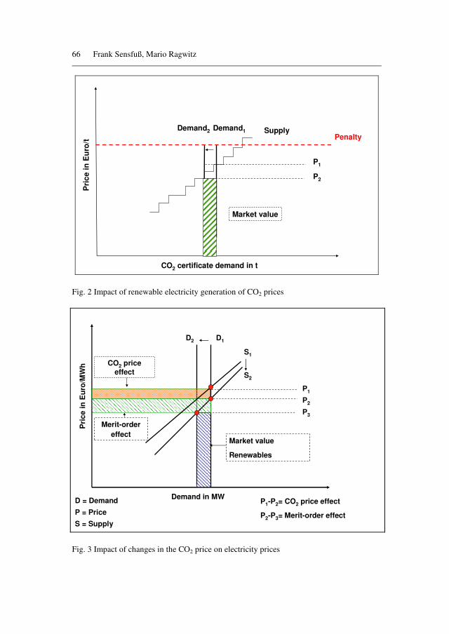
66 Frank Sensfuß, Mario Ragwitz
Demand2 Demand1 Supply
Pri
ce in
Eu
ro/t
CO2 certificate demand in t
P1
P2
Penalty
Market value
Fig. 2 Impact of renewable electricity generation of CO2 prices
D2 D1
S1
Pri
ce in
Eu
ro/M
Wh
Demand in MW
Market value
Renewables
Merit-order effect
P2-P3= Merit-order effect
D = Demand
S2
S = Supply
CO2 price effect
P1
P2
P3
P = Price
P1-P2= CO2 price effect
Fig. 3 Impact of changes in the CO2 price on electricity prices

An agent-based simulation platform as a support tool for the analysis of the interactions of
renewable electricity generation with the electricity and CO2 market 67
3 Model description
In order to analyze the effects that are discussed in the previous chapters a simulation model is required which has a sound basis in terms of fundamental data and representation of the techno-economic situation of real world markets. The PowerACE is simulation platform is developed for this purpose. The PowerACE simulation platform simulates important players within the electricity sector as computational agents. Among these are agents representing consumers, utilities, renewable agents, grid operators, government agents and market operators. Some players like utilities are modelled using several computational agents representing different functions within the company like trading or generation. The current ver-sion of the PowerACE model incorporates a spot market for electricity, a market for balancing power and a market for CO2-emssions. Since the goal of this paper is to analyse the impact of renewable electricity generation on spot market prices all other markets are deactivated for the simulation runs. An overview of the entire model and the main agents involved in the simulation is given in Figure 2. In gen-eral the simulation platform can be categorized in four modules dealing with: markets, electricity demand, utilities and renewable electricity generation.
CO2 Market
0
10
20
30
40
50
hour
Spotmarket
0
10
20
30
40
50
hour
Services
Industry+ Others
Household
Supplier
Contracts
TransportRenewable Agents
load
bids
Gridoperator-Trader
support
load
support
Generator
Supply Trader
merit-order
offer
bid
Primary Reserve Balancing Trader
offer
Gridoperator
bids
Plant DB
plant data
REG-Load DB
REG-Capacity DB
Investment Planner
new plant
offer
CO2 Trader
merit-order
offer
bid
CO2TraderSaving Potential
Industry DB
Load DB
Demand DB
Load-Prognosis
Investment Planner
new plant
offer
bid
co2 balance
load profiles
demand+equipment(HH)
Agents
data
Flows
Database
Markets
Demand
Renewables
Utilities
LegendSecondary Reserve
Minute Reserve
PumpStorageDB
PumpStorageTrader
offer bid
CO2 Market
0
10
20
30
40
50
hour
CO2 Market
0
10
20
30
40
50
hour
Spotmarket
0
10
20
30
40
50
hour
Services
Industry+ Others
Household
Supplier
Contracts
TransportRenewable Agents
load
bids
Gridoperator-Trader
support
load
support
Generator
Supply Trader
merit-order
offer
bid
Primary Reserve Balancing Trader
offer
Gridoperator
bids
Plant DB
plant data
REG-Load DB
REG-Capacity DB
Investment Planner
new plant
offer
CO2 Trader
merit-order
offer
bid
CO2TraderSaving Potential
Industry DB
Load DB
Demand DB
Load-Prognosis
Investment Planner
new plant
offer
bid
co2 balance
load profiles
demand+equipment(HH)
Agents
data
Flows
Database
Markets
Demand
Renewables
Utilities
LegendSecondary Reserve
Minute Reserve
PumpStorageDB
PumpStorageTrader
offer bid
Fig. 4 Structure of the PowerACE simulation platform

68 Frank Sensfuß, Mario Ragwitz
The realistic simulation of the impact of renewable electricity generation on
spot market prices requires extensive data. Therefore a central part of the simula-tion is to provide realistic data on electricity demand, renewable electricity genera-tion and the stock of power plants in Germany. The agents’ fundamental decisions are based on this data. An adequate dataset for the PowerACE simulation platform is provided by soft-links to various models. The ISI Load Model and the LEAP model provide load profiles and a long term development of the electricity de-mand. Since the central goal of this paper is the analysis of renewable electricity generation the provision of adequate load profiles for renewable electricity genera-tion is crucial. The ISI-PV (Sensfuß, 2003) and ISI Wind model (see also (Sensfuß et al., 2003); (Klobasa, Ragwitz, 2005b) generate these data for photovoltaic and wind energy on the basis of extensive meteorological data and assumptions on the regional distribution of wind turbines. The PERSEUS model Möst et al., 2005) can be used to provide a scenario for the future development of the German power plant portfolio and to calculate load profiles of electricity imports and exports. Additional information on the support of renewable electricity generation and dif-ferent sectors of electricity demand is stored in databases. Among these are infor-mation on company size, household size and household equipment levels in terms of electric appliances.
On the demand side the consumer agents representing the sectors household, industry, transport and service negotiate contracts with the supplier-agents repre-senting the sales department of utilities. In the given version of the model the sup-plier-agents purchase the entire electricity required by their consumers on the spot market. Thereby the supplier-agents are modelled as price takers.
Electricity supply is simulated by Generator-agents and Supply-Trader-agents. Generators get a daily updated list of power plants which is based on a detailed power plant database containing the most important parameters of more than 1200 power plants (capacity, costs, availability, technology, fuel). Generator agents check the availability of their power plants. The availability of power plants is de-termined by a uniform distributed random generator. Based on this information provided by the generators the traders can sell electricity generated by their power plants on the spot market.
Renewable electricity generation plays a growing role in the German electricity sector. According to the Renewable Energy Sources Act (Bundesministerium für Umwelt, Naturschutz und Reaktorsicherheit [BMU], 2004) the electricity gener-ated from renewable energy sources has to be bought by grid operators at guaran-teed feed-in tariffs. The renewable electricity is brought into the market by selling month-ahead base load blocks based on a prognosis of renewable electricity gen-eration which is sold to supplier-agents at the price of the feed-in tariffs. On a day-ahead basis a new prognosis of renewable electricity generation is calculated and the differences between the sold base-load block and the new day ahead hourly prognosis is traded on the spot market (E.ON, 2005). This task is carried out by the Gridoperator-Trader in the PowerACE simulation. In order to decrease the complexity of the market analysis envisaged in this paper the prognosis error of

An agent-based simulation platform as a support tool for the analysis of the interactions of
renewable electricity generation with the electricity and CO2 market 69
the projection of renewable electricity generation is set to zero, which means that the day-ahead prognosis matches the actual generation. Future analysis will take typical forecast errors into account.
∅=
+⋅⋅
+
+
⋅⋅+>++
⋅⋅+
+
⋅⋅+<−+
⋅⋅+
=
PG;MP;MG;Mi
otherwiseoezp
Piandoezp
ifs
oezp
Giandoezp
if),s
oezp
max(
p
i
i
ff
i
i,f
i
i
ff
i
i,f
hi
i
fi
ff
i
i,f
i
i
ff
i
i,f
hi
i
i
ff
i
i,f
h,i
∩⊂⊂∈
∈
∈0
η
ζ
η
η
ζ
ηϕ
ση
ζ
η
η
ζ
ηϕ
υη
ζ
η
Legend: Variables Unit Indices e = CO2-emission factor [t CO2/MWh] f = Fuel G = Set of base load power plants [None] h = Hour M = Set of all operation-ready power plants [None] i = Plant o = Variable operation and maintenance cost [Euro/MWh]
P = Set of peak load power plants [None] p = Price [Euro/MWh] s = Start-up cost of plant [Euro] z = CO2 price [Euro/t] η = Efficiency [%] σ = Number of scheduled hours per day [Hour] υ = Number of unscheduled hours per day [Hour] φ = Predicted price of spot market [Euro/MWh]
ζ = CO2 price integration factor [None]
Formula 1 Calculation of the bid price for power plants (see also Sensfuß, Genoese, 2006)
4 Calibration and evaluation of the developed model
Since the developed simulation platform is used provide quantitative results it is important have a thorough calibration and validation procedure. The central task of the developed simulation platform is the simulation of spot market prices in Germany. Therefore it seems to be important to compare the results of the devel-oped model to market prices on the German spot market EEX. This seems to be even more important if the enormous number of input data is taken into account which needs to be validated. Due to the availability of detailed data on renewable energy the years 2005 and 2006 have been selected for a detailed comparison of the market results. In 2005 and 2006 the complexity of the sector is increased due to the beginning of the European Emission Trading System.
70 Frank Sensfuß, Mario Ragwitz
The introduction of the European emission trading system creates the CO2 prices as a new input factor for the calculation of electricity prices. Since the emission permits have been allocated for free by the national allocation plan in Germany, an important question is how much of the CO2 price is integrated into the calculation of the bid price. In order to determine the likely CO2 price factors for the different power plants a case study has been carried out in cooperation with the University Karlsruhe. A detailed description can be found in Genoese et al. (Genoese et al., 2007). In the case study the CO2 price factors are varied for each fuel until the ordered market curve and the correlation shows the best fit to the real market prices on the German spot market. The result is that it is assumed that the CO2 price is integrated to 100 % into the calculation of the bid price of gas fired plants. In case of hard coal and lignite fired plants the factor reaches only 85 % and 70 %. This result is somewhat surprising since economic theory would expect that the price of every production factor is integrated to 100 % into the calculation of the bid price. A possible explanation for the lower price factors could be the al-location rule of grandfathering with ex post judgement where certificates which have not been used by a plant have to be given back at the end of the trading pe-riod. Ca. 15 % of the allocated emissions are subject to this rule. Another reason could be long-term take or pay contracts for fuels which could prevent a lower utilization of existing plants. The results of the comparison for the year 2005 are similar to those of the years presented above. Due to the higher price level the fil-ter is set to 120 Euro/MWh. As a consequence of the increasing number of hours with very high prices this filter excludes 159 hours from the analysis. The correla-tion of the filtered time series reaches 0.64. Again peak prices are generally higher in the real world market.
A similar calibration procedure is carried out for the year 2006. The resulting CO2 price factors for gas and hard coal reach 100 % for the year 2005. Exceptions are lignite fired plants. The best results can be reached for a CO2 pricing factor of 20 %. This result cannot be explained easily. One possibility could be that compa-nies want to keep the utilization of lignite plants on a high level for strategic rea-sons. Another reason could be caused by the fact that companies owning lignite power plants also own the related mines. Since lignite can hardly be transported for long distances due to its low energy content, lignite power plants and lignite mines are perhaps considered as one planning unit. In this case the total fuel cost of lignite power plants are no longer considered as variable cost, but as fixed cost since the mines are designed for a given output level. In a recent study it is stated that only ca 30 % of the fuel cost for lignite are variable mining costs (Energiewirtschaftliches Institut an der Universität zu Köln (EWI), Energy Envi-ronment Forecast Analysis (EEFA) GmbH, 2007). As a consequence the utiliza-tion of lignite power plants is likely to react only to a very limited extent to mod-erate CO2 emission prices. This is an aspect which could heavily affect possible emission reduction strategies in Germany since lignite fired plants are character-ized by the highest CO2 emissions. Furthermore electricity imports based on foreign nuclear or hydro plants could have some influence on the prices in times of low electricity demand which could have an impact on the calibration of the model. A closer analysis of this issue
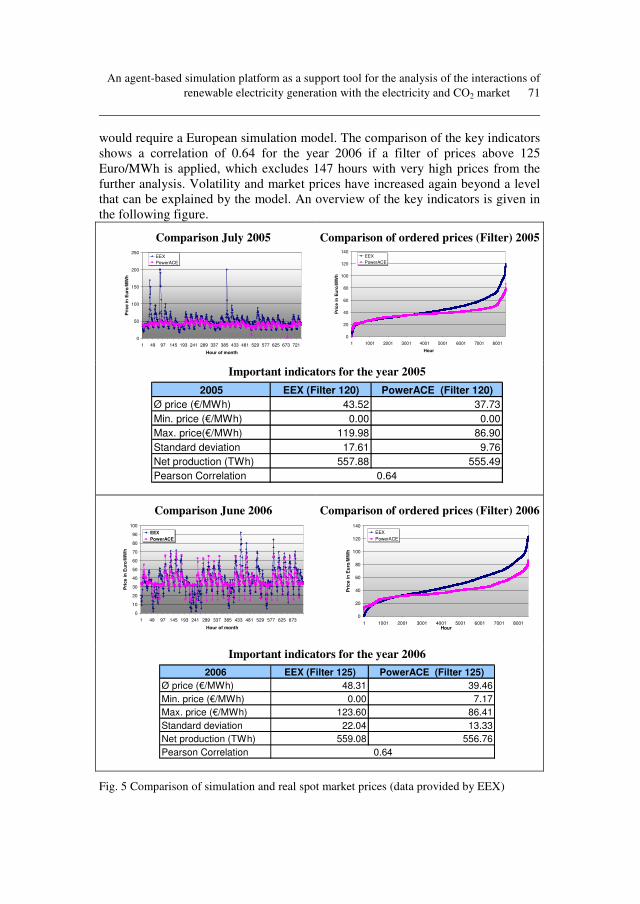
An agent-based simulation platform as a support tool for the analysis of the interactions of
renewable electricity generation with the electricity and CO2 market 71
would require a European simulation model. The comparison of the key indicators shows a correlation of 0.64 for the year 2006 if a filter of prices above 125 Euro/MWh is applied, which excludes 147 hours with very high prices from the further analysis. Volatility and market prices have increased again beyond a level that can be explained by the model. An overview of the key indicators is given in the following figure.
Comparison July 2005
0
50
100
150
200
250
1 49 97 145 193 241 289 337 385 433 481 529 577 625 673 721
Hour of month
Pri
ce in
Eu
ro/M
Wh
EEXPowerACE
Comparison of ordered prices (Filter) 2005
0
20
40
60
80
100
120
140
1 1001 2001 3001 4001 5001 6001 7001 8001
Hour
Pri
ce in
Eu
ro/M
Wh
EEXPowerACE
Important indicators for the year 2005
2005 EEX (Filter 120) PowerACE (Filter 120)Ø price (€/MWh) 43.52 37.73Min. price (€/MWh) 0.00 0.00Max. price(€/MWh) 119.98 86.90Standard deviation 17.61 9.76Net production (TWh) 557.88 555.49Pearson Correlation 0.64
Comparison June 2006
0
10
20
30
40
50
60
70
80
90
100
1 49 97 145 193 241 289 337 385 433 481 529 577 625 673
Hour of month
Pri
ce in
Eu
ro/M
Wh
EEXPowerACE
Comparison of ordered prices (Filter) 2006
0
20
40
60
80
100
120
140
1 1001 2001 3001 4001 5001 6001 7001 8001Hour
Pri
ce in
Eu
ro/M
Wh
EEXPowerACE
Important indicators for the year 2006
2006 EEX (Filter 125) PowerACE (Filter 125)Ø price (€/MWh) 48.31 39.46Min. price (€/MWh) 0.00 7.17Max. price (€/MWh) 123.60 86.41Standard deviation 22.04 13.33Net production (TWh) 559.08 556.76Pearson Correlation 0.64
Fig. 5 Comparison of simulation and real spot market prices (data provided by EEX)
72 Frank Sensfuß, Mario Ragwitz
5 Results
The calculation of the merit-order effect and the CO2 prices effect is a complex task requiring a thorough analysis which is not possible within this paper. How-ever the first important task for these analyses is to analyze the impact of renew-able electricity generation on the power plant operation. The central basis for analyses regarding the CO2 price effect of renewable electricity generation is the estimation of the CO2 savings caused by renewable electricity generation. In order to determine the impact of renewable electricity generation on the CO2 emissions in the German electricity sector the calibrated model is used to simulate the elec-tricity market for the years 2004, 2005, and 2006. Similar to the analysis of market prices presented in the previous section simulations are carried out for each year. The model calculates the CO2 emissions of each running power plant according to Formula 2:
;ev
h i i
fh,i⋅
⋅=∑∑
ηα
Legend: Variables Unit Indices e = CO2-emission factor [t CO2/MWh] f = Fuel v = Hourly electricity generation of plant [MWh] h = Hour α = Annual CO2 emissions [t] i = Plant η = Efficiency [%]
Formula 2 Calculation of the annual CO2 emissions in PowerACE
The resulting time series is calculated as average of the simulation runs in or-der to level out variations caused by the random variables used to simulate power plant outages. In a second step the same procedure is applied to 50 simulation runs without renewable electricity production supported by the feed-in tariff. Since the development of large hydro plants has not yet been affected by the renewable sup-port scheme, electricity production of large hydro plants is taken into account in both simulation settings. The resulting CO2 emissions are compared for both time series. An overview of the simulation results is given in Fig. 6.
Since PowerACE does not account for the additional CO2 emissions caused by partial load operation of conventional power plants due to renewable electricity generation an adjustment of the results is necessary. Based on an existing review of different approaches to the calculation of CO2 savings (Klobasa, Ragwitz, 2005a, a reduction factor of 10 % is assumed which is the highest value of the compared studies. The results of the corrected CO2 savings are presented in Table 1. Based on this comparison it can be stated that the CO2 savings calculated within this thesis represent a conservative calculation of the CO2 savings by renewable electricity generation.

An agent-based simulation platform as a support tool for the analysis of the interactions of
renewable electricity generation with the electricity and CO2 market 73
347 350 353
311 311 311
34.5 38.532.3
0
50
100
150
200
250
300
350
400
2004 2005 2006
Year
CO
2 em
issi
on
s in
Mt
PowerACE exl. renewables PowerACE incl. renewables Savings
Fig. 6 Simulated annual CO2 emissions of the German electricity sector
Table 1 Corrected CO2 savings by renewable electricity generation
Category Year
Excl.
EEG
Incl.
EEG
Partial
load
reduction
Corrected
savings
Renewable
Generation
Mt Mt % Mt TWh
CO2
emissions 2004 347.2 311.3 10 32.3 41.5
CO2
emissions 2005 349.5 311.2 10 34.5 45.5
CO2
emissions 2006 353.4 310.6 10 38.5 52.2
Although PowerACE allows for the calculation of CO2 savings on a very high
detail level, it seems to be important to compare the results of the calculated CO2 savings with the literature in order to evaluate the results. Klobasa and Ragwitz (Klobasa, Ragwitz, 2005a) provide an overview of existing studies and provide an own estimation of the CO2 savings in the year 2003. An overview of some studies
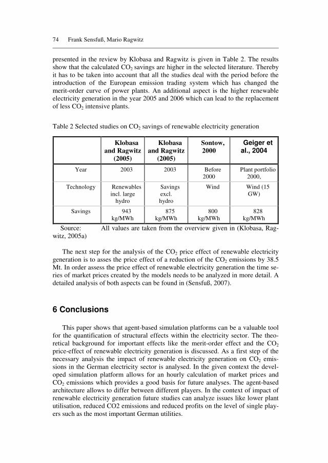
74 Frank Sensfuß, Mario Ragwitz
presented in the review by Klobasa and Ragwitz is given in Table 2. The results show that the calculated CO2 savings are higher in the selected literature. Thereby it has to be taken into account that all the studies deal with the period before the introduction of the European emission trading system which has changed the merit-order curve of power plants. An additional aspect is the higher renewable electricity generation in the year 2005 and 2006 which can lead to the replacement of less CO2 intensive plants.
Table 2 Selected studies on CO2 savings of renewable electricity generation
Klobasa
and Ragwitz
(2005)
Klobasa
and Ragwitz
(2005)
Sontow,
2000
Geiger et al., 2004
Year 2003 2003 Before 2000
Plant portfolio 2000,
Technology Renewables incl. large
hydro
Savings excl. hydro
Wind Wind (15 GW)
Savings 943 kg/MWh
875 kg/MWh
800 kg/MWh
828 kg/MWh
Source: All values are taken from the overview given in (Klobasa, Rag-witz, 2005a)
The next step for the analysis of the CO2 price effect of renewable electricity generation is to asses the price effect of a reduction of the CO2 emissions by 38.5 Mt. In order assess the price effect of renewable electricity generation the time se-ries of market prices created by the models needs to be analyzed in more detail. A detailed analysis of both aspects can be found in (Sensfuß, 2007).
6 Conclusions
This paper shows that agent-based simulation platforms can be a valuable tool for the quantification of structural effects within the electricity sector. The theo-retical background for important effects like the merit-order effect and the CO2 price-effect of renewable electricity generation is discussed. As a first step of the necessary analysis the impact of renewable electricity generation on CO2 emis-sions in the German electricity sector is analysed. In the given context the devel-oped simulation platform allows for an hourly calculation of market prices and CO2 emissions which provides a good basis for future analyses. The agent-based architecture allows to differ between different players. In the context of impact of renewable electricity generation future studies can analyze issues like lower plant utilisation, reduced CO2 emissions and reduced profits on the level of single play-ers such as the most important German utilities.

An agent-based simulation platform as a support tool for the analysis of the interactions of
renewable electricity generation with the electricity and CO2 market 75
References
Bundesministerium für Umwelt, Naturschutz und Reaktorsicherheit [BMU] (2004): Gesetz für den Vorrang Erneuerbarer Energien, http://bundesrecht.juris.de/bundesrecht/eeg_2004/gesamt.pdf, downloaded 10.04.2007. E.ON (2005): E.ON Windreport. http://www.eon-avacon.com/ContentFiles/Internet/ Downloads/E.ON_Netz_Windreport_2005.pdf. downloaded 15.01.2006 Energiewirtschaftliches Institut an der Universität zu Köln (EWI); Energy Environ-ment Forecast Analysis (EEFA) GmbH (2007): Energiewirtschaftliches Gesamt-konzept 2030 Szenariendokumentation vom 23.5.2007, Studie im Autrag von VDEW,BDI, DEBRIV,GVSt, VDN, VGB PowerTech und VRE. downloaded 23.06.2007 Geiger, B.; Hardi, M.; Brückl, O.; Roth, H.; Tzscheutschler; , P. (2004) CO2 -Vermeidungskosten im Kraftwerksbereich, bei den erneuerbaren Energien sowie bei nachfrageseitigen Energieeffizienzmaßnahmen, München: Lehrstuhl für Ener-giewirtschaft und Anwendungstechnik, Technische Universität München. Genoese, M.; Sensfuß, F.; Möst, D.; Rentz, O. (2007): Agent-Based Analysis of the Impact of CO2 Emission Trading on Spot Market Prices for Electricity in Germany. In: Pacific Journal of Operations Research, 3 (3), pp. 401-423. Klobasa, M.; Ragwitz, M. (2005a) Gutachten zur CO2 Minderung im Stromsektor durch den Einsatz erneuerbarer Energien, Karlsruhe: Fraunhofer Institut für Sys-tem- und Innovationsforschung. Klobasa, M.; Ragwitz, M. (2005b): Simulation der Windeinspeisung in Deutschland und Rückwirkungen auf den Kraftwerksbetrieb. Proceedings of IEWT 2005 - Ener-giesysteme der Zukunft: Herausforderungen und Lösungspfade Die Zukunft der Energiewirtschaft im liberalisierten Markt : 4. Internationale Energiewirtschaftsta-gung an der TU Wien, Wien, Österreich. Möst, D.; Genoese, M.; Rentz, O. (2005): Sensitivitätsanalyse der CO2 Emissionen im Elektrizitätssektor bei Gas- und Zertifikatspreisvariationen. In: Zeitschrift für Energiewirtschaft, 05 (4), pp. 301-312. Rathmann, M. (2007): Do support systems for RES-E reduce EU-ETS-driven elect-ricity prices? In: Energy Policy, 35 (1), pp. 342-349. Sensfuß, F. (2003): Entwicklung einer Prognose des Lastprofils der Stromeinspei-sung erneuerbarer Energien bis 2020, Praxisarbeit, University of Flensburg. Sensfuß, F. (2007): Assessment of the impact of renewable electricity generation on the German electricity sector An agent-based simulation approach, Dissertation, Universität Karlsruhe (TH), Karlsruhe 2007.

76 Frank Sensfuß, Mario Ragwitz
Sensfuß, F.; Genoese, M. (2006): Agent-based simulation of the German electricity markets-An analysis of the German spot market prices in the year 2001-. Procee-dings of the "9. Symposium Energieinnovationen", Graz, Austria15.02.2006-17.02.2006. Sensfuß, F.; Ragwitz, M.; Wietschel, M. (2003): Fluktuationen der Windenergie und deren Vorhersagbarkeit bei einem verstärkten Ausbau des Off-Shore Anteils in Deutschland bis 2020. Proceedings IEWT, Vienna 2003. Sontow, J. (2000): Energiewirtschaftliche Analyse großtechnischer Windstromer-zeugung, Dissertation, Institut für Energiewirtschaft und Rationelle Energieanwen-dung, University of Stuttgart. Walz, R. (2005): Interaktion des EU Emissionshandels mit dem Erneuerbare Ener-gien Gesetz. In: Zeitschrift für Energiewirtschaft, 29 (4), pp. 261-269.

A modelling tool for interaction and correlation in demand-side market behaviour 77
A modelling tool for interaction and correlation in demand-side market behaviour
Jörg Bremer, Stefan Andreßen, Barbara Rapp, M. Sonnenschein and M. Stadler
Carl von Ossietzky Universität Oldenburg and OFFIS Institute for Information Technology, Oldenburg
Summary. We present an agent-based software environment for modeling and simulation of adaptive consumers responding to dynamic electricity pricing. It has been specially designed for scenarios involving household customers. Households can be modeled down to the layer of single appliances, even taking into account presence and price awareness of inhabitants. Modeled utilities can calculate prices from different factors using different methods. The focus of investigations con-ducted is the analysis of household load shifting potential under different tariffs and different negotiation strategies. Keywords: agent-based modeling, electrical load shifting, household consumers
Acknowledgement
We thank EWE AG, a regional utility in northern Germany for funding large portions of the work described herein in conjunction with the subproject ‘Adaptive Consumers’ embedded in the project DEMS for exploring management of decen-tralised energy systems.
1 Introduction
It is important to keep the balance between electricity consumption and elec-tricity production at all times. This is usually done by supplying cost intensive balancing power without taking into account the potential of the demand-side. The major factors responsible for high marginal costs are peak loads that usually are met using expensive peak load generation facilities, and grids dimensioned to sup-port peak loads. Thus, it is necessary to minimise peaks while at the same time op-timally utilise base load plants. Peak load reduction can be achieved either by power conservation methods or via load shifting on the consumer side which is also suited to address the problem of

78 Jörg Bremer, Stefan Andreßen, Barbara Rapp, M. Sonnenschein and M. Stadler
optimal utilisation of base load plants. Load shifting can be achieved by methods of demand side management involving direct control of appliances or indirect con-trol by addressing the inhabitants of households through time varying tariffs re-flecting the marginal costs of electricity production. The maximum load shifting potential of households has still got to be examined and also the percentage of load shifting potential activated by different tariff signals or other control signals is currently not well known.
This calls for a model of power consumption reflecting electricity demand down to the device level also encompassing human price awareness, presence pro-files, as well as seasonal influences and thereby the elasticity of demand. Further-more, if different negotiation strategies shall be examined w.r.t. to the achievable matching between load and production, the models must also support federations of consumer agents negotiating with utilities.
In recent years, a lot of research has been done in the field of optimizing elec-trical load through demand side management methods. We limit a short overview here on attempts related to multi-agent technologies. The HomeBots approach [Ygge and Akkermans 1996, Ygge 1998] is based on the idea of an electronic market place where utilities and devices (e.g. electrical heaters) are trading small amounts of energy to match the current demand with the supply. Prices are fixed by a market based approach. A similar approach is proposed by [Wedde et al. 2006] focussing more on the technical aspects of implementing a distributed mar-ket place. Both attempts aim for a completely new, distributed method of demand-supply matching as well as electricity pricing that is not oriented at our current system of energy supply. They do not incorporate planning agents scheduling en-ergy demanding tasks to optimally match between supply and demand.
In [Penya 2006] also a retail market place for electricity is investigated, where a reverse combinatorial auction is used as a method for electricity pricing and load shifting. This model consists of two different agent-based systems: one system for price fixing between utilities and consumers, and another system for scheduling of demand tasks, This approach results in very high communication costs - it has not been tested for ‘real world’ scenarios.
For these reasons we decided to develop our own agent-based modelling and simulation platform ACDC (adaptive consumers for dynamic cost models) aiming at dynamic pricing for consumers which is presented in this paper. A preliminary version of the ACDC frameworks has been described in [Sonnenschein et al. 2006].
This paper is organised as follows: After a short introduction to the domain of load management in households we explain the architecture and some basic con-cepts of our agent based simulator ACDC in chapter two. In chapter three different hypothetical scenarios for negotiation between consumers and a utility are intro-duced. These scenarios are implemented in the ACDC framework and demon-strate its flexibility.

A modelling tool for interaction and correlation in demand-side market behaviour 79
1.1 Load shifting within households
Load shifting is a basic mechanism for adapting load curves so as to reduce marginal costs of electric power supply. Load shifting within households is based on their inhabitants behavior and in their equipment. Thus, we have to account for both.
There are different types of appliances. Controlling appliances control an envi-ronmental factor within the household. Examples of this appliance type are fridges, air conditions, heaters and boilers. Appliances for spontaneous use are switched on and off by persons, following their needs of daily living. TV sets, lighting and cooking equipment are examples for this type. Finally, programmed appliances after having been switched on follow a given program and have a pre-dictable power consumption sequence. It is important to note that the mechanisms of load shifting differ substantially for the appliance types.
The load shifting potential of appliances for spontaneous use is only dictated by the needs of persons that vary due to many factors as circadian rhythms and social events. Usage patterns for this appliance type are influenced by the presence of persons within a household and circadian rhythms but can be modified through social events or other causes. The only way of exploiting a load shifting potential is by modifying people’s behavior, for example by varying electricity costs and thereby exploiting price awareness.
Load shifting potential for programmed appliances is also driven by human be-havior, but to a lesser degree. Usage of dishwashers, washing machines and alike devices is not always spontaneous and often planned. For instance, people might refrain from using their washing machine late in the evening due to noise. Also usage of programmed appliances is mostly delayed until after a certain payload has been reached. A very interesting fact concerning those appliances is, that they are equipped with controllers allowing to delay operation after starting the device. This can be interpreted as a user wanting the appliance to terminate its program at a latest given point in time. Taking this as a hook for integrating a scheduler al-lows for load to be shifted to a moment when electricity consumption is most de-sirable due to sufficient resources or low prices. Note, that the load can be shifted forward in time.
Controlling appliances control a physical property (e.g. temperature) to stay within bounds defined by the persons living in a household. For that purpose they do not depend from human interaction. By intelligently exploiting the range be-tween the bounds, load can be shifted. For instance, the temperature within a fridge’s cooling compartment may be allowed to vary between 5°C and 8°C. Whenever the upper bound is reached, the fridge’s cooling aggregate is started. It stays on as long as the lower temperature bound is not under-run. Using an intelli-gent fridge controller, a fridge’s thermal storage capacity can be exploited as to prepone or postpone the cooling aggregate’s activity and thereby shifting load for time spans of about an hour [Stadler et al. 2007].
Single persons are reflected in our consumer models by their presence profiles. The usage patterns for household appliances derived from human behaviour are modeled through usage profiles.
80 Jörg Bremer, Stefan Andreßen, Barbara Rapp, M. Sonnenschein and M. Stadler
2 ACDC – a modelling and simulation framework for cost adaptive electricity consumption scenarios
A model in our ACDC framework consists of an electricity supplier (power company) calculating real-time prices for electricity, different classes of electricity consumers (households) modeled in essential by their scheduling mechanism of energy consuming tasks, and a communication protocol between consumers and the electricity supplier. Power plants and electric generators as e.g. wind turbines are modelled only as sources for time series of available electrical energy.
2.1 System architecture
The simulation and modeling environment ACDC consists of the basic build-ing blocks depicted in figure 1. A purpose-built modeling tool allows graphical construction of models and parametrisation of models and their components. As-pects that cannot be graphically defined (e.g. interaction protocols and rule sets for defining tariff calculation) may be composed from within a simple built-in text editor. Once defined, parametrised models are stored as XML-files within the sys-tem’s scenario repository.
Figure 1. General component architecture In standalone mode, these scenarios are read by a single simulation engine as soon as the ‘start simulation’ button is clicked. In distributed mode, multiple simulation clients may fetch scenarios from the scenario server as soon as they run out of a job. The generation time series, tariff time series and load timeseries are stored within a relational database at simulation time. From there, they can be retrieved via reporting adapters, either by standard reporting tools or by a live time series display and analysis tool currently under construction.

A modelling tool for interaction and correlation in demand-side market behaviour 81
The simulation engine is built around the Repast framework [North et al. 2006] offering a comprehensive infrastructure for agent-based modelling and simulations including mechanisms for communication and synchronisation. Agents in this framework do not pursue their tasks in real-time but execute concurrently based on a common global simulation time. Developing the ideas from [Rölke 2004] this allows for partitioning a complex process of interaction into independent, loosely coupled software entities.
Inter-agent communication is based upon the Repast Framework’s event han-dling mechanism. To guarantee for extensibility, the flow of communication is specified within replaceable interaction protocols implemented through a control unit and a monitoring unit. Communication channels are configurable by allowing for specification of bandwidth or message-delay by the modeller and they are separated from the communication methods used (e.g. messages or handshakes).
Aside from messages, the behavior of agents may be influenced by events. Whenever an event occurs, an agent may react to it or choose to ignore it. The simulator allows for specification of contents, purpose and other properties of messages and moreover it offers a broadcasting functionality that can be used for agents sending a message to multiple receivers.
2.1.1 Agent types and agent structure
Each agent within a simulation represents an entity within our scenario. The type specific functionality of an agent is structured in a number of type specific modules. Helper classes needed within modules or agents are represented by items which are not limited to representing data but may also have functionality as-signed to them.
We need three types of agents for modeling the scenarios required for our ana-lyses. Utility agents represent utilities calculating electricity prices from different inputs comprising wind power predictions, electricity stock market prices at the European Energy Exchange, and also electricity consumption predictions. All of these inputs may be calculated from outputs of consumer agents or from utility agent modules providing interfaces to Excel files and comma separated value files.
Electricity prices can be negotiated between utility agents and consumer agents in several rounds. The information exchange is performed by sending tentative pricing time series from the utility to its consumers, and by sending predicted con-sumption time series calculated for a given pricing time series from consumers to their utility.
Consumer agents represent households that consume electricity taking into ac-count given pricing information. Consumption is aggregated from the set of ap-pliances present within a household.
Both, the activities of programmed appliances and controlling appliances are scheduled by per-agent schedulers using different strategies. Each consumer agent consists of an internal model with a scheduler for adaptive resource planning. Specific points in time for switching appliances on or off are derived from infor-mation about probable usage periods. Additionally, the probability of usage might be a function of electricity prices. It is then the schedulers task to alter the periods

82 Jörg Bremer, Stefan Andreßen, Barbara Rapp, M. Sonnenschein and M. Stadler
of activity for each appliance according to a given tariff with the objective of mi-nimising overall costs. For this purpose different optimisation techniques are in-volved [Sonnenschein et al. 2006]: the behaviour of controlling appliances is al-tered by ant colony optimisation; planning of programmed appliances is driven by a tabu search algorithm. As an example, figure 2 depicts the internal structure of an agent representing electricity consumers. Device models, scheduler, metering and control unit are modules, while human behavior and consumption statistics are delivered by items.
2.2 Configurability
The ACDC tool consists of a simulator engine and an optional graphical user interface. Both are highly configurable in favor of adjustability to specific needs. The simulator engine was implemented as a standalone desktop application based on the Spring Framework [Johnson 2007]. This layered Java/J2EE application framework includes a non-invasive lightweight container that is able to link loosely-coupled components to a complex system.
The simulator engine’s configuration is done in terms of XML. The Spring In-version of Control (IoC) processes configuration options, such as the prefered per-sistence technology, the list of databases to access, or the option of declarative transaction management, and so on, given in a simple and intuitive XML format. At runtime the configuration file is processed by the container. In case of a dis-tributed simulation on more than one machine and hence different simulator en-gines the underlying configuration can be shared across the network. This allows for configuring different decentral simulator engines either identically or inde-pendently of each other.
load
scheduler
control
unit load forecast
metering &
consumption
statistics
device
models
information about
time-varying
usage probability
schedule
human-
price
awareness
tariff
information flow
control signal
Figure 2. Internal model of adaptive consumers

A modelling tool for interaction and correlation in demand-side market behaviour 83
Configuring scenarios for simulation mostly takes place in terms of XML. Each scenario configuration is divided into two separate parts: Firstly, all agents partici-pating in a simulation, their associated functionality, all required communication channels as well as desired choreographies are listed. All these entities are re-quired to achieve the target-settings by simulating a scenario. This first brief part of configuration is passed to and evaluated by our custom-developed parser. The second part of the configuration file contains a series of Java object definitions that are required for simulation as well. Syntactically this part corresponds to a format processable by the IoC container out-of-the-box. At runtime the container performs instantiating or sourcing application objects (e.g. agents, modules, items etc.), configuring these objects, and assembling the dependencies between them.
Most of the participating agents require different external definitions to satisfy their functions. Such external definitions like profiles of presence, price awareness or rule sets have to be specified with external tools and can be used for simulation via referencing such files in the scenario configuration. In addition, individual in-habitant types can be modeled with individual behaviour in using certain appli-ances wich is also be influenced by their individual price awareness. Hence a cor-related behaviour can be achieved.
Individual modelling of each single agent in large scenarios is a tedious and er-ror-prone work. Thus, our system exploits a concept for factory driven generation of heterogeneous agent populations for large scenarios. Individual agents of such a population with mutually distinct traits and behaviour as well as diverse equip-ment may be described by means of specialized XML-based definitions. Special-ized, so called factory agents take use of these descriptions and generate the actual definitions of a large number of agents according to the given stencil.
In connection with developing appropriate structures for such descriptions of distinct model parts and agents for use in factories the following problems had to be taken into account:
Prefabricated model components must be available from different libraries in order to avoid double definitions, for reuse, and ease of modelling.
Modelling of well defined varieties within model components must be possible in order to support heterogeneous agent populations; e. g. the definition of a re-frigerator with an arbitrary but well defined distributed power input of its com-pressor.
Dependencies between model parts must be part of their definitions. E. g. sup-posed a specific class of household agents possesses appliance A with a given probability P1. Now it should be possible to define that if a specific instance of these agents actually possesses appliance A than it also possesses appliance B with probability P2.
In order to support a flexible integration of functional elements into the struc-ture of our XML-based model description, we adapted the principles of custom elements. Custom elements are a commonly used build-in programming means within JavaServer Pages (JSP) wich allow for program generated parts within fixed template HTML-code. So, we adapted this idea and enriched our XML-based factory definitions with similar structures for dynamic content. That means that our parsers for XML factory definitions are capable of identifying dynamic
84 Jörg Bremer, Stefan Andreßen, Barbara Rapp, M. Sonnenschein and M. Stadler
content by means of namespace, interpreting such elements and replacing them with the generated output of the corresponding implementation. Figure 3 sche-matically shows the chosen approach.
In JSPs action elements represent dynamic actions that are executed at runtime when a JSP is requestet [Bergsten 2002]. In analogy, our dynamic XML elements are executed at parse-time. It is the factory parsers task to add a given number of agent definitions to a given scenario definition. In this way an agent description in a factory serves as a fuzzy stencil for the definitions to be inserted into the sce-nario. For each inserted instance the dynamic elements' action classes are exe-cuted. The individually generated output of these action classes then replaces the respective element within the stencil resulting in distinguishing agent definitions derived from a single prototype.
Figure 3. Scheme for factory based agent generation
As yet, we use these dynamic elements to realize control structures, for an in-
tegration of numerically derived content, i. e. specifically distributed values, and

A modelling tool for interaction and correlation in demand-side market behaviour 85
script generated. In order to pass information between different executions of ac-tions as well as between different simulation runs, two different scopes are pro-vided: scenario and simulation. Data in the scenario scope is only valid for a sin-gle scenario simulation run whereas the simulation scope allows for passing data from one simulation run to another; listing 1 shows an example of modelling a batch simulation with a growing number of agents for each run.
Listing 1. Example of JSTL within XML In addition, we integrated support for dynamic attribute values. The Expression
Language (EL) is defined by the Java Standard Tag Library (JSTL) specification [Delisle 2002]. EL expressions can be used to set attributes to dynamic values. Whereas the JSTL implementations only allow for a use with action elements our implementation allows for setting attributes of arbitrary (including non-dynamic) elements to dynamically generated values. A shared context allows for exchanging variable values between dynamic elements and EL expressions, or rather, their implementations. Another advantage resulting from our implementation is an easy way of extending the original standard language by integrating own implementa-tions of additional functions as shown in listing 2 where the non EL function weighted_pick is used within an EL expression to choose from the given choices with respective probabilities.
Listing 2. Example of EL extensions Factory driven generation of scenarios together with dynamic definitions and
commonly used profile definitions enables us to model scenarios with a well de-fined correlation between different actors within a scenario as well as dependen-cies between different simulations runs. For example, in a scenario with multiple different agents representing varying instances of different classes of households generated by factories, it is still possible to model a correlation in the usage time of the refrigators by providing them with the same usage profile. In this way, all households will show a certain similarity in behaviour concerning the usage of the refrigator (i. e. opening the door, filling in warm food, etc.) while each of these appliances is separatedly treated, or rather, optimized according to the settings of the simulation.
<ae:if test="${empty counter}"> <ae:set var="counter" value="0" scope="simulation"/> </ae:if> <ae:set var="counter" value="${counter+5}" scope="simulation"/>
<class name="growingExample" count="${counter}">[...]</class>
<appliance ref=${weighted_pic(fridgeA, 20, fridgeB, 80)} />

86 Jörg Bremer, Stefan Andreßen, Barbara Rapp, M. Sonnenschein and M. Stadler
3 Definition of three scenarios for negotiating tariffs between a utility and its customers
Negotiation in each scenario presented in this chapter is based on feedback loops between a utility and its customers. The feedback to a tariff given by a util-ity is a load forecast. We view tariffs as a control signal leading to a load shift re-sulting in a better balance of electricity consumption and electricity production. This approach differs from the approach described in [Wedde et al 2006] where the feedback of a customer contains pricing information instead of information on load.
3.1 Independent customers negotiating with a utility
The standard scenario used for conducting analyses of tariff induced load shift-ing of household customers is based on the assumption that customers act inde-pendently of each other, each reacting on tariff prognoses. Figure 4 shows a sim-plified structure of the scenario with an emphasis on agent communication.
Figure 4. Hierarchical communication scheme Each day at a specified time, the utility begins tariff negotiations. A single nego-tiation round is split into the following steps: (1) The utility issues an initial tariff prognosis for the next day based upon
the predicted costs of electricity, the input from wind power and a total ex-pected load (based on prior experience).
(2) Loop until break criterion is reached a. Consumer agents optimize the schedule of their device activities
based on the predicted tariff and issue a load prognosis. b. The utility agent calculates a new tariff based on the predicted
load and the facts already known at calculation time of the initial tariff.

A modelling tool for interaction and correlation in demand-side market behaviour 87
(3) The last predicted tariff is sent to the consumers as final tariff; monitored household consumption is measured and integrated into the utilities load ex-pectation for future days.
The break criterion may be based upon the number of negotiation rounds or on the trend observed in the difference between desired load curves and achieved load curves. If the difference grows, it is assumed, that at least a local optimum had been reached.
Usually the tariff for one day is divided into time slices of 15 minutes and these tariffs are mainly examined in our work, but it is also possible to examine differ-ent time periods. With our tool it is also possible to take into account certain cal-culation times and communication delays decoupled from simulation time. In this way, different time frames for such negotiations can be examined.
This approach is well-suited to explore the maximum achievable load shifting for a given population of consumers and a given tariff calculation method. How-ever, using this interaction protocol, tariff valleys will result in load peaks. This is due to a synchronised behaviour of agents neither having knowledge of each oth-ers reaction nor having any means of knowledge about the actions necessary to purposefully change their device activity plans with respect to the global optimiza-tion goal to reduce load peaks.
3.2 Probability based negotiation between federated customers and their utility
An extension of the standard scenario described in section 4.1 has been de-signed to reduce the disadvantages of independently negotiating consumers.
Consumers negotiating following a probability based strategy are indirectly aware of other consumer’s presence, i.e. they do not communicate with any other consumer, but assume the existence of other consumers scheduling their devices to minimise their electricity costs. In this negotiation type, consumers agree to the fact that independent cost optimization for all consumers result in load peaks, and they agree to contribute in a fair way to avoid this effect. For this purpose, they use a probabilistic approach to attenuate their cost minimisation, resulting in a co-operative behaviour between consumers and between consumers and the utility. This means a partial abandonment of local benefits in favour to allow a better match between electric load and production curves. The reduced load peaks lead to lower marginal costs for electricity supply and result in lower consumer prices in the long term.
The probability based negotiation is based on a modification of the signal ‘strength’ computed for each time slice of tariffs. This signal strength is compared with a randomly generated threshold value calculated separately by each consumer agent. The comparison of the signal strengths and the locally computed thresholds is used by consumer agents to calculate a fictitious tariff only used for device scheduling purposes but not designating electricity costs. To construct this ficti-tious tariff, a so called base tariff is modified by each agent during each subse-quent negotiation round as follows:
If the local threshold is greater than the modification signal strength for a time slice, the base tariff’s corresponding value is replaced by the time slice’s value of
88 Jörg Bremer, Stefan Andreßen, Barbara Rapp, M. Sonnenschein and M. Stadler
the tariff issued by the utility agent during the current negotiation round. Other-wise the base tariff’s time slice value is kept. In that way each customer agent constructs an individual tariff as input to their device activity scheduler resulting in a modified device activity plan.
The base tariff is a helper tariff which holds the costs that occurred in a time slice at the beginning of a price increase or decrease tendency of tariffs published by the utility agent during previous negotiating rounds.
In the probability based negotiation scenario the assumption of homogeneous consumers is made. All consumers behave the same way regardless of their rela-tive contribution to electricity consumption. Shifting load from a given time slice yields different results, depending on the consumer’s contribution to total con-sumption. This can lead to inadequate load shifting. In addition to that, the ran-domized threshold only guarantees for fairness of load shifting distribution be-tween agents, if the number of consumer agents is big enough.
First simulation runs show that the probability based negotiation indeed results in a better matching between electricity consumption and electricity production, if the signal strength is increased relatively slowly between negotiating rounds. Rapid increase of signal strength often results in a customer’s over-reaction and therefore can be a reason for insufficient load shifting. Besides achieving the main goal of improving the match between consumption and production, the probability based negotiating has the advantages of having both, low computational perform-ance requirements and communication requirements.
Figure 5. Simulation result from probability based negotiation

A modelling tool for interaction and correlation in demand-side market behaviour 89
Figure 5 depicts the correlation between electricity costs and appliance usage
for three households resulting from simulating probability based negotiation for a duration of two days. There are two appliances per household. One of those has a low power rating and is of use during morning and evening hours. The other has a high power rating and can be used throughout the day.
The diagram shows, that the appliance type with high power rating is only acti-vated when electricity costs are low. Moreover, due to probability based schedul-ing of appliance activities, not all three households activate their appliances with high rating during the same time slots with low electricity costs. Instead, activity of those appliances is distributed over the available time slots. Note that the first and last time slot of each 24 hour period are not used, since appliance activity has been forbidden during the night.
The appliance type with smaller rating cannot be scheduled to be active during low cost electricity phases, because those phases do not overlap with the allowed per-day activity periods for this appliance type.
3.3 Communicative approach for federated customers negotiating with utility
We assume that an even better match between electricty consumption and elec-tricty production can be achieved by federated planning, and by dropping the as-sumption of homogeneous consumers. Federated planning is conducted by a spe-cial agent named concentrator. Each concentrator is assigned to a number of consumer agents and communicates with the utility on their behalf. Communica-tion between consumers and concentrators is bidirectional. The concentrator re-ceives tariffs from the utility agent.
Figure 6. Integrating the concentrator (1) Just as for the probability based approach customers agree that coordinated
planning of device activity results in better overall pricing conditions and is therefore worthwhile even if temporary disadvantages in accessibility to low priced tariff time slices can occur for single customers.

90 Jörg Bremer, Stefan Andreßen, Barbara Rapp, M. Sonnenschein and M. Stadler
Within a single negotiating round the following steps are executed: (1) The utility issued tariff is used by each customer to schedule device activity
independently of other consumers following mere personal benefits. (2) The resulting local device activity plan is sent to the concentrator. (3) After receiving all single device activity plans the concentrator builds an indi-
vidual tariff for each consumer agent based on that device’s activity plan and on the calculated signal strength.
(4) The concentrator sends the individual tariffs to its associated consumers. (5) Finally, based on their special tariffs the customer reschedule their device ac-
tivity and provide a load prognosis for feedback needed by the utility.
In detail the segment wise calculation of the individual tariff by the concentra-tor depends on the signal strength, the consumer’s reaction strength and a rating of fairness. This can be found in [Andreßen 2007]. First results for this scenario are currently evaluated.
4 Conclusion and further work
We presented a flexibly configurable agent-based tool for modelling tariff based load shifting scenarios. It has already been extended to scenarios involving direct control of devices and can be easily extended to distinct market based sce-narios for demand side management within the electricity domain. It still has to be tested whether the tool can also successfully be applied to modelling and simula-tion problems within other domains.
We showed that different inter-agent negotiation scenarios can be realised. The concept of thick agents extensible through function modules has proven particu-larly useful. The novel architecture of ACDC allows for introduction of com-pletely new agents simply by coding the functionality using the tool’s class framework without changing existing code and changing XML configuration files.
The downside of the flexible approach is the complexity of our tool. Together with the multiple configuration options it results in a long learning periods for both, users and developers.
The tool is currently used for carrying out analyses of load shifting potentials described in the introduction. Before the tool will be used in additional scenarios, e.g. in load shifting under market influences including settings with multiple utili-ties and combined producers / consumers, we will improve its runtime efficiency. Further possible improvements include the introduction of an extended model checker, providing a better guidance when modelling new scenarios, a module for time series analysis and a context-sensitive editor with auto-completion for reduc-ing the time required to construct new orchestration protocols and agent factory definitions.

A modelling tool for interaction and correlation in demand-side market behaviour 91
References
St. Andreßen: Entwicklung und Analyse von Kommunikationsszenarien zur Koordi-nation der Stromnachfrage unter dynamischen Stromtarifen. Diploma Thesis, Uni-versity of Oldenburg, Dept. of Computing Science, 2007 H. Bergsten : Java Server Pages, O'Reilly & Assosiates Inc. 2002, 2nd ed. P. Delisle (ed.): JavaServer Pages Standard Tag Library, SUN Microsystems, Inc.,
2002 R. Johnson et al.: The Spring Framework - Reference Documentation, Version
2.0.7 North, M.J., Collier, N.T. and Vos, J.R. (2006): Experiences Creating Three Imple-mentations of the Repast Agent Modeling Toolkit. ACM Transactions on Modeling and Computer Simulation, Vol. 16, Issue 1, pp. 1-25 Y. Penya: Optimal Allocation and Scheduling of Demands in Deregulated Markets, PhD Thesis, Technical University of Vienna, Austria 2006 Rölke, H. (2004): Modellierung von Agenten und Multiagentensystemen - Grundla-gen und Anwendungen. In Moldt, Daniel (ed.): Agent Technology: Theory and Ap-plication, Vol 2. Logos Verlag, Berlin, Germany M. Sonnenschein, M. Stadler, B. Rapp, J. Bremer, St. Brunhorn: A Modeling and Simultion Environment for Real-Time Pricing Scenarios in Energy Markets. In: Tochtermann, K., Scharl, A. (Eds.): Informatics for Environmental Protection - Envi-roInfo Graz 2006. M. Stadler, W. Krause, M. Sonnenschein, U. Vogel: The Adaptive Fridge – Com-paring different control schemes for enhancing load shifting of electricity demand. In: Hryniewicz, O., Studzinski, J., Romaniuk, M. (Eds.): 21st Conference on Infor-matics for Environmental Protection - Enviroinfo Warsaw 2007 H. F. Wedde, S. Lehnho, E. Handschin, O. Krause: Autonomous Real-Time Management of Unpredictable Power Needs and Supply. ECRTS'06, IEEE Com-
puter Society, 2006. F. Ygge, H. Akkermans: Power Load Management as a Computational Market. Proceedings of the 2nd International Conference on Multi-Agent Systems ICMAS’96, Kyoto, Japan, 1996 F. Ygge: Market Oriented Programming and its Application to Power Load Management. PhD Thesis, Department of Computer Science, Lund University,
1998 .


Success determinants for technological innovations in the energy sector – the case of photovoltaics 93
Success determinants for technological innovations in the energy sector – the case of
photovoltaics
Nils Roloff, Ulrike Lehr, Wolfram Krewitt, Gerhard Fuchs, Sandra Wassermann, Wolfgang Weimer-Jehle, Bernd Schmidt
Nils Roloff, Ulrike Lehr, Wolfram Krewitt: DLR, Institut für Technische Thermodynamik, Abteilung für Systemanalyse und Technikbewertung, Pfaf-
fenwaldring 38-40, 70569 Stuttgart, first name.last [email protected]; Gerhard Fuchs, Sandra Wassermann, Wolfgang Weimer-Jehle: Institut für Sozialwis-
senschaft, Abteilung für Technik- und Umweltsoziologie, Seidenstr. 36, 70174 Stuttgart, first name.last [email protected]; Bernd Schmidt:
Juvenellstr. 45, 90419 Nürnberg, [email protected]
Summary In response to the growing challenges of climate change and resource scarcity energy from renewable sources will have to play a significant role on fu-ture energy markets. Therefore, significant efforts from the industry will be neces-sary in terms of innovative processes and products to fulfill the needs of a future energy mix and the success determinants for these technological innovations are of considerable interest. The paper outlines the results of a study that focuses on the different aspects of in-novation in the photovoltaic industry. Innovation research suggests that innovation processes take place in systems of highly interdependent actors. Agent-based modeling provides a suitable tool for the analysis of the various effects of actors’ choices, strategies and dynamic behavior. The study concentrates on the main ac-tors within the innovation system “Production and Application of Photovoltaic Technology Systems”: producers, PV system operators (households, farmers etc.), research institutes and universities, banks, interest groups and trade associations, installation firms, and government. Within these groups different characteristic features exist and each type is represented by one agent. Research institutes, for instance, can be oriented towards either applied or more theoretical research. This will affect their respective strategies on cooperativeness and knowledge genera-tion. A variety of different types of producers is observable in the photovoltaic market, e.g. fast growing companies, new branches of established energy produc-ers or off-mainstream innovative SMEs, which are characterized by different learning strategies and different goals. Households have different objectives and motives for the purchase of a certain type of PV system and their market behavior feeds back to industry and research. Viewing innovation processes from an agent-based perspective allows innovative computational analysis of the organizational interdependencies between the relevant actors. It goes beyond standard analysis of

94 Nils Roloff, Ulrike Lehr, Wolfram Krewitt, Gerhard Fuchs, Sandra Wassermann, Wolfgang Weimer-Jehle, Bernd Schmidt
innovation processes in that it tries to combine agent based and systemic consider-ations. In particular the response of actors to different energy policy measures, their dynamically emerging behavior and their related implications on innovation in the field of PV is described. The transferability and limits of the case study’s re-sults are analyzed. Keywords: agent-based modeling, innovation, photovoltaics
1 Introduction
European energy markets currently undergo significant changes from centra-lized monopolistic markets to a more competitive environment with a lot of differ-ent participants. Additionally, the challenges from climate change and environ-mental issues have to be met. Renewable energy will play a significant role on future energy markets as the new targets from the European Commission show (KOM (2007) 1). To reach these targets several support mechanisms have been developed and have led to high dynamics in the renewable energy industry. Apart from environmental goals, the support policies aim at economic develop-ment and technological change. The German feed-in law, for instance, has already triggered the rapid development in the German wind industry and in the photovol-taic industry. But it is widely agreed that still a lot of innovation is needed for technologies to provide clean electricity at affordable cost at a large scale for the future.
Success factors in an innovation system hinge on a wide array of determinants. They differ depending on the innovation phase, the technology and the actors, in-stitutions and participants in the innovation system. The technological system for solar cells exhibits some very interesting characteristics: Firstly, the technology as such has been known for more than 100 years by now (Green 2000). However, the technological development was dominated by ‘science-based experimentation’ un-til the 1990s. Solar cells were first used for extraterrestrial applications during the so called ‘Space Age’ (1958 to 1973). Later on they were also used for consumer electronic products as well as for off-grid power systems (1974 until mid-1990s). Nevertheless the role of photovoltaics with regard to the supply of energy re-mained quite limited until Japan and Germany started their first demand-oriented programs during the 1990s. These initiatives and successive programs and regula-tive changes eventually led towards a significant growth of the PV-industry and therefore to an expansion of the whole technological system (Jacobsson et al. 2002). Secondly, as the technology evolved, the motifs of actors changed and new actors have been attracted to the field. This and the interdependence of political in-fluence, consumer behavior, research and development led to the chosen modeling approach. Agent based modeling (ABM) seems to be a very suitable approach in a highly interdependent system that evolves in a non-equilibrium and self-organizing fashion.
The structure of the contribution is as follows. After this introduction, chapter 2 outlines the theoretical background of the analysis. We have drawn from three
Success determinants for technological innovations in the energy sector – the case of photovoltaics 95
disciplines – innovation research, agent based modeling and energy system analy-sis and technology assessment. Chapter 3 gives an overview of the model and first results will be presented in chapter 4. Chapter 5 concludes.
2 Theoretical Background
2.1 Innovation research
To capture the multi-faceted structure of the innovation system we work from a rather wide definition. Innovation in this analysis means all artifacts, processes, ideas and strategies that successfully change routines and are implemented in spe-cific contexts of use, which can be changed in turn through the innovation. This definition is wider than some to be found in the literature in the sense that it not only comprises the invention of a new process or technology but also its diffusion . Therefore, the analysis does not stop at the mere analysis of patent data or the in-troduction of a new technology, but takes the whole innovation system with its in-trinsic feed-back loops into consideration. The interdependence between actors, their co-operation and spill-overs play an important role (see e. g. Carlsson and Stankiewicz 1991, Edquist 2001, Lundvall and Johnson 2001 and Malerba 2006). Accordingly, the process of innovation is not understood as a linear sequence but rather as a non-linear, highly interactive process as proposed by Kline and Rosen-berg (1986) or Rothwell (1995).
The importance of innovations for social change, international competition, structural change and economic growth has been analyzed quite successfully in the last decade. However, how and why innovation comes about and what triggers it or slows it down is still an open question. There is evidence, that knowledge is the most important input in the process of innovation; the importance of know-ledge in certain innovative industries has been empirically shown (cf. Dosi 1988, Hullmann 2001). Sparks of innovation emerge through the interplay of different forms of heterogeneous knowledge: their confrontation, combination, fusion, transformation. Different schools of thought describe the accumulation and the distribution of knowledge within the firm, in the economic sector and in innova-tion system differently.
From an individualistic perspective the analysis focuses on the entrepreneur, who decides about access to knowledge in the firm (Hauschildt 2004). Evolutio-nary economics takes a more comprehensive approach and sees the firm as know-ledge storage and as part of a wider organizational system (Fagerberg et al. 2005). The distribution of knowledge affects the innovativeness of a firm, but the type of knowledge in the firm and the innovation system also has a large influence. Argy-ris and Schön (1978) argued that the capacity to innovate would depend on the ability of organizations to bridge individual and collective forms of knowledge. Nonaka and Takeuchi (1995) proposed that the secret of the knowledge-creating

96 Nils Roloff, Ulrike Lehr, Wolfram Krewitt, Gerhard Fuchs, Sandra Wassermann, Wolfgang Weimer-Jehle, Bernd Schmidt
company would reside in its capacity to master the different modes of conversion of tacit and codified forms of knowledge. Cook and Brown (1999) have suggested that the true spark of innovation lies in the ‘generative dance between possessing and practicing knowledge’.
As pointed out earlier, our approach takes the whole innovation system into account. The Innovation Systems approaches most clearly follow the principles of evolutionary economy. An “Innovation System” can be defined as the cluster of institutions, policies, and practices that determine a nation’s, region’s or sector’s capacity to generate and apply innovations (Carlsson and Stankiewicz 1991, Lundvall et al. 2001, Malerba and Orsenigo 1997).
The Innovation Systems approach has achieved high visibility and political in-fluence, but has been controversially discussed. Rammert (2002), for instance, ar-gued that the approach lacked micro-foundations and would not reflect the path dependence of innovation formation due to habit, norms and institutions. Rammert argues further that innovation systems currently are undergoing a transition from sequentially organized systems to fractionally structured networks. Though such a system is different for each innovation – a thought that is reflected in the term “bi-ography” of an innovation – Rammert, together with Hage and Hollingsworth (2000) or Amin and Cohendet (2004) assumes that the number of actors from dif-ferent backgrounds enhance the likelihood of strong innovation activities and their success in the system. However, the more the analysis focuses on the individual biographies, the less the approach becomes suitable for more general recommen-dations and results. Therefore, in our approach we try to balance the analysis of individual motifs with more structural and systematic assessments. An additional challenge is to keep the structural approach sufficiently flexible to be able to an-swer the question “How are innovations generated, shaped and institutionalized by distributed innovative activities in heterogeneous innovation networks?”
2.2 Multi-agent based simulation
To analyze the innovation processes in the technological system for solar cells the agent based modeling approach is used. In contrast to the models of conven-tional simulation (e.g. system dynamics), in which participants are modeled in an aggregated top-down approach, agent based models consist of different individual decision-making agents. These bottom-up built agents interact with each other and thereby influence the development of the whole system. This allows modeling of distributed problem solving processes in a more realistic way. Hence, agent based simulation allows to transfer complex systems from reality into a model, which can be used to analyze dynamic processes and alternative strategies within the sys-tem.
Actors or rather stakeholders in the real world are represented as ‘agents’ in the respective model. Agents can represent individuals as well as entities on a higher aggregation level, like e.g. a company, a political party or a research organ-ization. To make full use of the benefits of the agent-based simulation approach,

Success determinants for technological innovations in the energy sector – the case of photovoltaics 97
actors and agents as their representatives in the model are described in terms of the following characteristics:
• Dynamic environment: actors live in a changing environment to which they adopt.
• Individuality: each actor is characterized by its own individuality, which means that he/she has its specific status, options for action and targets. The actor’s status may change over time because of its own internal momentum or because of external constraints.
• Goals and strategies: Each actor has individual goals, which he/she strives to achieve. To achieve the goal, the actor has the capability to plan a course of events. The actor develops strategies for target-oriented action.
• Communication and interaction: Actors have the capability to communicate and to interact with one another, which can lead both to co-operation and com-petition.
• Environmental model: the environmental model describes how the actor perce-ives the real world. The environmental model is created by inputs from the real world and by cognitive processes. In general it reflects not only factual infor-mation, but also mental attitudes. An actor’s action is always determined by his/her environmental model. An actor thus does not act on the basis of an
'objective' reality, but on how he/she perceives reality.
It is expected that agent based simulation offers distinct advantages in analyz-ing innovation processes, as it allows a specific and detailed representation of re-lated actors and stakeholders. It thus facilitates the simulation of the dynamic processes resulting from interaction between actors with different sets of goals or values. Cooperation in complex adaptive systems can create emergent behavior, which occurs when the behavior of a system is more complicated than the simple sum of the behavior of its components. Traditional modeling techniques such as linear programming do not include emergent behavior. The ability to model emer-gent behavior is therefore considered a specific advantage of agent-based simula-tion to analyze innovation processes.
Regarding the analysis of innovation processes or rather innovation systems several theoretical studies already exist. These studies focus on different aspects related to innovation in general like e. g. the transfer of knowledge (März et al. 2006, Wersching 2007, Pyka et al. 2006), the diffusion of innovations (Steyer and Zimmermann 2001) or the effects of different diversification strategies of firms (Dawid and Reimann 2003). But nevertheless, very few attempts have been made so far to apply agent-based modeling to simulate the influence of multiple stake-holders on the innovation processes in a specific technological system. First ex-amples are analyses of innovation processes in urban water infrastructure systems (Kotz and Hiessl 2005, Schwarz 2007) or the examination of the diffusion process of fuel cell vehicles (Schwoon 2003).
Because of the crucial importance of the interdependences between the rele-vant actors in innovation processes, and the dynamics of emergent behavior, we
98 Nils Roloff, Ulrike Lehr, Wolfram Krewitt, Gerhard Fuchs, Sandra Wassermann, Wolfgang Weimer-Jehle, Bernd Schmidt
consider multi-agent based simulation as an innovative, promising and powerful computational analysis tool which can be successfully used in the field of innova-tion research. Open issues which still need further consideration are questions concerning the empirical validation of the models and how far multi-agent based sys-
tems can cope with the representation of medium to long term time periods (Richiardi 2004, Windrum et al. 2007).
3 The Model
3.1 Basic Assumptions
The success of an innovation depends on the one hand on an adequate configu-ration of people, objects and ideas and on the other hand on the combination of the personally embodied knowledge and the materially incorporated technological know-how (Rammert 2002). It is important to note that a realistic approach to the understanding of innovations has to be a dynamic, “biography” or “career” oriented one. Innovations are not a one stop affair. Rather innovations develop more or less quickly over time. Some innovations take their time. In certain sec-tors innovations are rather small scale and incremental while in others they may in fact be destroying old and creating new structures. The firm is without any doubt an important agent in the generation of innovations. Whether it is in fact the cen-tral agent is not so much a theoretical than an empirical question. The decisive impulses can result from producer-client/customer relations (e.g. von Hippel 1988, 2004) or can even be the product of public initiatives (Edquist 2004).
The types and structures of relationships and networks differ from sectoral sys-tem to sectoral system, as a consequence of the features of the knowledge base, the relevant learning processes, the basic technologies, the characteristics of de-mand, key links and dynamic complementarities. Thus, in a sectoral system pers-pective, innovation and production are considered to be processes that involve sys-tematic interactions among a wide variety of actors for the generation and exchange of knowledge relevant to innovation and its commercialization. Interac-tions include market and non-market relations that are broader than the market for technological licensing and knowledge, inter-firm alliances, and formal networks of firms (Carlsson 1994, Breschi and Malerba 1997). Only recently a research tra-dition is slowly evolving that takes these sectoral characteristics of innovation
processes at its heart.6 The notion of a Sectoral System of Innovation (SSI) de-parts from the traditional concept of sector used in industrial economics because it examines other agents in addition to firms, places great emphasis on knowledge, learning and sectoral boundaries, focuses on non-market as well as market interac-
6 see Malerba 2004 for a state of the art overview. For case studies see also Brac-
zyk/Fuchs/Wolf 1999, Fuchs 2004, Fuchs and Koch 2005.

Success determinants for technological innovations in the energy sector – the case of photovoltaics 99
tions, and pays much attention to institutions. Innovation is considered as a process that involves continuous and systematic interactions among a variety of actors.
A SSI is thus composed of a set of agents carrying out market and non-market interactions for the creation, production and sale of sectoral products (Malerba 2004:10).
(a) Any sector can be first of all characterized by its specific knowledge base,
technologies and inputs. One way to categorize these elements was proposed by Malerba and Orsenigo (1997). They distinguish roughly between oppor-tunity and appropriability conditions, degrees of cumulativeness of technol-ogical knowledge and characteristics of the knowledge base.
(b) Actors, Institutions, and Policies. A sector consists of a set of heterogeneous
actors that are organizations or individuals (e.g. consumers, entrepreneurs, scientists). Organizations may be firms (e.g. users, producers and input sup-pliers) or non-firm organizations (e.g. universities, financial organizations, government agencies, trade unions or technical associations), including sub-units of larger organizations (e.g. research and development – R&D – or production departments) or groups of organizations (e.g. industry associa-tions). Actors are characterized by specific learning processes, competen-cies, beliefs, objectives, organizational structures and behaviors. They inte-ract through processes of communication, exchange, cooperation, competition and command.
(c) Institutions. Actors’ cognition, actions and interactions are shaped by institu-
tions, which include norms, routines, common habits, established practices, rules, laws, standards and so on. They may range from the ones that bind or impose enforcements on actors to the ones that are created by the interaction among actors (such as contracts); from more binding to less binding; and from formal to informal (such as patent laws or specific regulations versus traditions and conventions). Many institutions are national (such as the pa-tent system), while others may be specific to sectoral systems, such as sec-toral labor markets or sector-specific financial institutions.
(d) Demand. The focus on users, customers, public procurement and regulation
puts a specific emphasis on the role of demand in sectoral systems and in the innovation process. Demand is not seen as an aggregate set of similar buy-ers, but as being composed of heterogeneous agents the interaction of which with producers is shaped by institutions.
The starting point of the model development has been the definition of the ac-
tors that are relevant for the innovation system under scrutiny. The model at its current stage exhibits all the important characteristics with all the agents. As agents we include the most important actors in the innovation system: Producers

100 Nils Roloff, Ulrike Lehr, Wolfram Krewitt, Gerhard Fuchs, Sandra Wassermann, Wolfgang Weimer-Jehle, Bernd Schmidt
of PV-systems, consumers/system operators, R&D-institutes, government, trades, interest groups and banks.
The agents „producer“, “R&D-institute“ and „consumer“ are at the core of the model. Producers not only produce, but also market and sell PV-systems. They observe the markets, build expectations on demand development and change their respective strategy according to their own market success. Likewise, investment follows expectations on market development. Furthermore, they have their own R&D departments and work on own innovations. For this purpose they make use of publicly-available knowledge and also buy knowledge externally, e. g. via li-censes. Additionally, they contribute to the overall knowledge base by generating new knowledge within the course of their R&D-activities.
In addition to that, “producers” have the opportunity to use capital for three different purposes: they can improve the efficiency of production with respect to resources and/or labor, they have the possibility to invest in human capital and hire more skilled labor and they can acquire additional knowledge either from the market for licenses or from stepping up internal research and development ex-penditures. “Producers” try different investment measures and develop their strat-egy according to their market success.
Research and development institutes and firms receive funding from public budgets (agent “government”) and from private budgets, i.e. other firms. The R&D institutes produce knowledge. Public knowledge is disseminated via publi-cations, conference contributions and other scientific exchange platforms. Proprie-tary knowledge is patented and then sold to firms. The amount of research results depends on the available capital, human resources, network activities and co-operations. With respect to human resources the research and development agents compete on the labor market with the producers for skilled and qualified labor.
Regarding the “consumers” of PV-modules, one could state that their respec-tive motivation to buy a PV-system has changed considerably over time. 25 years ago, people who bought PV-modules were either enthusiastic about the technolo-gical aspects or convinced of the environmental benefits. Economic aspects did not – and could not, given the state of the technology at that point in time – play a role. Since then two developments occurred. Firstly, the effectiveness of the sys-tems improved and the yields increased substantially. Secondly, the monetary re-turns have been improved by the market liberalization and the German feed-in ta-riff system (EEG). The liberalization of the German electricity market provided the legal framework for market access for independent producers. In addition to that, the German feed-in tariff system with the obligation of net operators to con-nect any producer of electricity from renewable energy sources (RES) to the grid and with fixed (profitable) tariffs for electricity from RES led to the development of a new, profit-oriented demand sector.
Therefore, the demand side agents have to reflect this variety of motifs. Ac-cordingly, attainable return on investment, stable conditions from the legal frame-work, interest in environmentally safe investment, technological thrill and support of renewable energy are constituent parts of the utility function of the “consum-ers”.

Success determinants for technological innovations in the energy sector – the case of photovoltaics 101
The role of banks (as a subcomponent of the agent “producer”) and the trades
is less active in the system. They are modeled as bottlenecks for capital and labor inputs in installation. Nevertheless, their activities influence the possibilities of supply and demand as well as the number of PV-systems that can be installed dur-ing certain time periods.
Due to the large influence of the (political) framework conditions at least for the German development, the agent “Government” is important in the model. However, the political decision process is not modeled as such. The government gives money for R&D, provides investment subsidies, sets the feed-in tariff and also grants credits with low interest rates. These variables are affected by the gov-ernments’ information level that is sustained by other departments (e.g. the targets for GHG), NGOs and trade associations and the firms. Additionally, the agents provide information themselves that facilitate trade activities. Figure 1 gives a schematic representation of the model.
Fig. 2. Structure of the model
4 Results
The detailed structure of the single agents in the model allows for an analysis of their behavior in the light of different assumptions. However, thus far, our model only includes one agent of each type, therefore competition between, for in-stance, two different producers cannot be modeled as of yet. This is an issue of fu-ture research.
Nevertheless, individual strategies can be modeled and the agents individually exhibit plausible reactions. Furthermore, the interesting interactions and feed-back reactions can be modeled using different components together. The following firstly focuses on individual strategies of the “R&D-institute” agent and shows

102 Nils Roloff, Ulrike Lehr, Wolfram Krewitt, Gerhard Fuchs, Sandra Wassermann, Wolfgang Weimer-Jehle, Bernd Schmidt
two experiments. Secondly, a small subsystem consisting of this agent, the firms’ agent and the consumers is used to validate the technology push effect that is well-known from the literature.
4.1 Individual strategies
As already mentioned, knowledge is a central element for innovation processes, especially with regard to science-based industries like the PV-sector. Accordingly, knowledge generating entities like R&D-institutes play a significant role in the technological system for PV systems. Hence, it is important to analyze the effects of certain biographic influences on knowledge output in the R&D-Institutes. Two R&D institutes with different focuses are considered. While the first one is more oriented towards applied research the other one leans towards ba-sic research. Each is calibrated with the data of a relevant existing institute of the photovoltaic sector. In order to analyze the behavior of the R&D agent it is inter-preted as an insulated system and is decoupled from the model as a whole. The structure of the agent is given in figure 2.
Join
t p
roje
ct
fun
din
g
Producer
HumanCapital
HumanCapital
Capital
Capital
ProprietaryKnowledge
PublicKnowledge
Producer
Government
Capital
Gra
du
ates
Mig
rati
on
Joint projectfunding
Third-party funds
Public project funding
Institutional funding
Rea
l cap
ital
:d
egra
dat
ion
by
agei
ng
Lab
or
cost
s
Migration
Knowledge-generation
Deg
rad
atio
n b
yag
ein
g
Graduates
Framework cond.
Labormarket
Framework cond.
Cooperations
Framework cond.F
un
din
gco
mp
osi
tio
n
Fu
nd
rev
enu
es
Deg
rad
atio
n b
yag
ein
g
Fig. 3. Internal structure of the “R&D”-agent
The key process inside this agent is “Knowledge-generation”. The production rate depends on two prerequisites: “Human Capital” (workforce) and “Capital”
Success determinants for technological innovations in the energy sector – the case of photovoltaics 103
(cash and equipment). “Capital” is fed by direct public funding, by company con-tracts and by indirect public funding via joint projects. “Capital” decreases due to the payment of wages and the ageing of equipment. The specific knowledge pro-duction rate increases if more equipment is accumulated. The agent employs addi-tional workforce if sufficient funds are available, providing that there is no lack of interested graduates. On the other hand, employees are dismissed if funds are in-sufficient. With respect to workforce, the R&D institute competes with producers and the general labor market: graduates may prefer other employers if the labor market is in strong condition. Furthermore institute employees may migrate.
Two types of explicit knowledge are produced. Public knowledge can be used by every agent without any precondition. Proprietary knowledge must be bought by other agents, with the exception of the producer who funded the corresponding project. The shares of the knowledge types depend on the relations in funding: public funding produces public knowledge, third party funds generate proprietary knowledge and joint project funding yields a mixture of both.
Co-operation with producers, a major issue in innovation research, causes an ambivalent, complex impact on the agents. Strong co-operation increases the effi-ciency of knowledge production. On the other hand, it stimulates migration to-wards producers, hindering the R&D institute by moving away workforce and im-plicit knowledge, but at the same instant promoting producers.
The two experiments look at idealized biographic types of institutes. The first experiment takes the example of a large non-university research institute, created in 1985 on a low level. The following biographical characteristics were used as model input:
- focus on applied research, - strong co-operation with industry, - public funding has increased until 1990, then stagnated, - increasing success in 1990’s in raising industry funding and, later,
joint project funding and - a high scientific reputation, yielding unlimited availability of gra-
duates.
The results of the simulation are given in figure 3. For a tentative calibration with empirical data we used data on the Fraunhofer-Institut für solare Energiefor-schung (Fraunhofer Institute for Solar Energy Systems - ISE) in Freiburg, Germa-ny. Its structure resembles the idealized type.
104 Nils Roloff, Ulrike Lehr, Wolfram Krewitt, Gerhard Fuchs, Sandra Wassermann, Wolfgang Weimer-Jehle, Bernd Schmidt
Human Capital (persons)
Public knowl.: rate of production (units/a) Cumulated public knowledge (units)
0
15
30
45
1985 1990 1995 2000 2005
0
100
200
300
1985 1990 1995 2000 2005
0
40
80
120
160
1985 1990 1995 2000 2005
Fig. 4. Applied non-university research institute: model results (solid lines) and empirical data of the ISE (squares).
The model satisfyingly reproduces the data on the development of the work-
force. Decreases in the workforce at the beginning of the 90s in the empirical data from ISE can be explained by a crisis in the institute (among other things a new competitor had been founded). So far the model does not include any of these changes.
The difference between the simulated data and the empirical measurements concerning the production of public knowledge until mid 90s result from the fact that the empirical data only include peer-reviewed articles. The model, on the oth-er hand, purposefully includes any type of public knowledge, including research results that are published in reports and non-reviewed publications (discussion pa-pers, gray literature). For later years data and simulated results merge, because in-ternational standards for publishing performance gradually catch on.
The second experiment analyses a middle-sized university institute with me-dium co-operation with the industry and a strong focus on basic research. As in the first experiment, we assume that the institute started in 1985 at a low level. Again a set of biographical characteristics was used as external drivers of the agent’s development:
- strong focus on basic research, - public funding increased first, then stagnated at the beginning of the
1990s, - medium co-operation with industry, - spin-off of an institute in the late 80s including staff transfer,
Success determinants for technological innovations in the energy sector – the case of photovoltaics 105
- acquisition of industry funding only started a couple of years ago, but
took a very dynamic development, - recruitment of new graduates is recently limited due to sharp compe-
tition from private firms and - a recent shift of the institute’s main working fields, including a poli-
cy of workforce reduction in the dropped fields.
Figure 4 shows the results of the simulation in comparison with empirical data. The empirical data for this tentative calibration are obtained from the Institut für physikalische Elektronik (Institute for Physical Electronics - IPE) at the University of Stuttgart, Germany, which resembles the idealized institute modeled. The accordance of the calculated human capital with the empirical data is fore-most due to the model input. It is not a test of the model quality, therefore. How-ever, the good reproduction of the development of the knowledge production (number of peer-reviewed articles as empirical data) is encouraging. The observed decrease of the number of published articles in more recent times proved to have complex causes. Obviously the decrease of workforce plays a role, but it isn't suf-ficient to explain the whole effect. Sensitivity analyses showed that the production of public knowledge also considerably decreases if the workforce reduction policy is removed. Almost half of the effect is due to demanding tasks for the industry (competition with proprietary knowledge) and to the limitations of the institute to acquire new personnel in a sufficient amount.
0
10
20
30
40
50
1985 1990 1995 2000 2005
0
10
20
30
40
1985 1990 1995 2000 20050
5
10
15
20
1985 1990 1995 2000 2005
Human Capital (persons)
Public knowl.: rate of production (units/a) Proprietary knowl.: rate of production (units/a)
Fig. 5. Medium size university institute: model results (solid lines) and empirical data of the IPE (squares) (solid squares right bottom: 3-year average of the empir-ical data).

106 Nils Roloff, Ulrike Lehr, Wolfram Krewitt, Gerhard Fuchs, Sandra Wassermann, Wolfgang Weimer-Jehle, Bernd Schmidt
These experiments show that the R&D agent is suitable for modeling bio-
graphic determinants of different R&D institutes. The results allow for sensible deductions concerning the behavior of the R&D institutes. However, data for em-pirical validation and calibration currently are incomplete and rather sketchy. Fu-ture work will be dedicated to the strengthening of the empirical data base and will focus on more and different research institutes in the PV sector. As has been pointed out, the current status of the model does not allow explicit modeling of in-teractions of different types of the same agent. For future work, different co-operative strategies between agents will be interesting to model.
4.2 Interdependence between key agents
Based on the experience with the simulation experiments described above, pro-totypical elements of all agents were merged for simulations with the whole mod-el. The following experiment is an example of the dynamic behavior of the model. The experiment analyses the “technology push” hypothesis. This hypothesis fol-lows the assertion that increasing public funding for the support of research will lead to accelerated innovation activities. To verify the hypothesis, we need two simulation runs. The first run represents the reference, because we want to show changes from an increase of public support with respect to some status quo, i.e. a reference case. The second run of the model includes the increase and the system’s reaction on this additional capital for research. Comparing the results of the two runs shows the effects of the technology support policy. Figure 5 shows the re-sults.

Su
ccess determ
inan
ts for tech
no
logical in
no
vatio
ns in
the en
ergy secto
r – th
e case of
ph
oto
vo
ltaics 107
Fig
. 6: A
naly
sis of th
e ‘techno
log
y p
ush
’-simulatio
n ex
perim
ent
"Producer": Efficiency of PV-modules
0
5
10
15
20
25
2 4 6 8 10 12 14 16 18 20Years
%
Reference 'Technology Push'
"Producer": Trend of earnings
0
1
2
3
4
2 4 6 8 10 12 14 16 18 20Years
Mio
. €/
a
Sales (reference) Sales ('Technology Push')Earnings (reference) Earnings ('Technology Push')Costs (reference) Costs ('Technology Push')
"R&D-institute": Knowledge
0
20
40
60
80
100
2 4 6 8 10 12 14 16 18 20Years
Un
its
of
kno
wle
dg
e
Public knowledge (reference)
Proprietary knowledge (reference)
Public knowledge ('Technology Push')
Proprietary knowledge ('Technology Push')
"R&D-institute": Capital Flow
0
100000
200000
300000
400000
2 4 6 8 10 12 14 16 18 20Years
€/a
Public project funding (reference)Third-party funds (reference)Public project funding ('Technology Push')Third-party funds ('Technology Push')Joint project funding (reference and 'Technology Push')

108 Nils Roloff, Ulrike Lehr, Wolfram Krewitt, Gerhard Fuchs, Sandra Wassermann, Wolfgang Weimer-Jehle, Bernd Schmidt
The increase of public funding at T=5 leads to a significant increase in the produc-tion of knowledge compared to the reference case. Since public funding primarily enters the production of public knowledge, the R&D agents shift their preferences from the production of proprietary knowledge to the production of public know-ledge. Therefore, proprietary knowledge decreases as a reaction to the monetary increase. However, the production of both types of knowledge increases on the long run due to more capital being available for both uses.
Producers profit from the increase in knowledge production, because they can use this knowledge as an input to their own R&D departments. The larger supply of (public) knowledge yields earlier product and process improvements compared to the reference case.
Technological change accelerates and yields increasing demand as the respec-tive agent reacts to the improvement of the PV-systems. Furthermore, the produc-ers react upon their market success and also obtain a larger profit due to process innovations which result in sinking productions costs. Capital stock increases at the producers and can be spent on the different uses described in chapter 3.
The experiment yields results that support the technology push hypothesis. Higher public funding accelerates the innovation activities. Additionally, a variety of feed-back loops reinforce the positive effect. The model reacts in a plausible way to an external shock that is modeled singular and discontinuous. The model is robust enough to deal with this type of external shocks and exhibits an accelera-tion of the innovation indexes.
5 Conclusions
The aim of this paper was to present an agent-based model for the analysis of innova-
tion processes in the photovoltaic industry. In order to be able to examine the success factors for innovations as well as the
effects of policy measures it is necessary to understand how the innovation system under scrutiny is influenced by the behavior of different stakeholders and their re-spective interactions. Therefore, the stakeholders that are considered important are treated as agents in our model. Each agent is characterized by its individual goals, specific strategies and behavioral rules. The (dynamic) interdependences between the agents are also taken into account. After the implementation of the agents each one has been calibrated with empirical data.
As the first experiments on the basis of a decoupled agent (“R&D-institute”) show the specific behavior of stakeholders can be modeled. Since the results of these simulation runs indicate that the model is already suitable for modeling bio-graphic determinants of different R&D institutes the link between empirical re-search and agent-based modeling seems to be possible.
Apart from that the interactions between the agents and the respective influ-ences on innovation processes can also be simulated on the basis of our model. Regarding the effects of discrete external influences the simulation model already

Success determinants for technological innovations in the energy sector – the case of photovoltaics 109
generates plausible results as the outcomes of the simulation run described in chapter 4.2 illustrate.
Since the focus here was on the individual strategies of the different stakehold-ers and also on their non-market interactions our model only includes one agent of each type. Therefore, market processes as competition between different produc-ers or technologies cannot be modeled adequately as of yet. Nevertheless, we be-lieve that the first results discussed in this paper demonstrate that the effects of the dynamic interactions between stakeholders on innovation processes (in the photo-voltaic industry) can be analyzed using agent-based simulation.
Given the already mentioned limitations of the current model there is still room for further improvements. Based on the developed structure more agents of each type have to be included such that analyses of the economic behavior of the agents as well as more detailed investigations of the non-market activities become possible. Additionally, the empirical validation of the model will be a key issue. Finally, the response of the stakeholders or rather agents to different policy meas-ures will systematically be examined by simulating different scenarios on the basis of the calibrated model. These simulation runs will provide insights into the suc-cess determinants of innovation and will support the future development of inno-vation policies as well as their implementation.
Acknowledgements: This research has been supported by the VolkswagenStif-tung, Germany in their program on “Innovation processes in the economy and the society”.
References
Amin, A.; Cohendet, P. (2004): The Architecture of Knowledge. Firms, Capabilities, and Communities. Oxford University Press, Oxford. Argyris, C.;Schön, D. (1978): Organizational Learning: A Theory of Action Perspec-tive. Addison-Wesley, Reading. Breschi, S.; Malerba, F. (1997): Sectoral systems of innovation: technological re-gimes, Schumpeterian dynamics and spatial boundaries. In: Edquist, C. (ed.): Sys-tems of innovation. Pinter, London. Carlsson, B. (1994): Technological Systems and Economic Performance. In: Dodgson, M.; Rothwell, R. (eds.): The Handbook of Industrial Innovation. Edward Elgar, Aldershot/Brookfield, pp. 13-24. Carlsson, B. and R. Stankiewicz (1991): On the nature, function and composition of technological systems. In: Journal of Evolutionary Economics, 1(2), pp. 93-118. Cook, S. D. N.; Brown, J. S. (1999): Bridging Epistemologies: The Generative Dance between Organizational Knowledge and Organizational Knowing’. In: Or-ganization Science, 10(4), pp. 381-400.

110 Nils Roloff, Ulrike Lehr, Wolfram Krewitt, Gerhard Fuchs, Sandra Wassermann, Wolfgang Weimer-Jehle, Bernd Schmidt
Dawid, H.; Reimann, M. (2003): Diversification: A Road to Inefficiency in Product Innovations?, CEM Working Paper 2003/63, University of Bielefeld. Dosi, G. (1988): Sources, Procedures, and Microeconomic Effects of Innovation. In: Journal of Economic Literature, 26, pp. 1120-1171. Edquist, C. (2001) The System of Innovation Approach and Innovation Policy: An account of the state of the art. Lead paper presented at the DRUID Conference, Aalborg, June 12-15, 2001. Online: http://www.druid.dk/conferences/nw/paper1/edquist.pdf (accessed: 06-02-2007). Edquist, C. (2004): The Fixed Internet and Mobile Telecommunications Sectoral System of Innovation: Equipment Production, Access Provision and Content Provi-sion. In: Malerba 2004, pp. 155-192. Fagerberg, J.; Mowery, D. C.; Nelson, R. R. (eds.) (2005): The Oxford Handbook of Innovation. Oxford University Press, Oxford. Green, M. A. (2000): Photovoltaics: technology overview. In: Energy Policy, 28(14), pp. 989-998. Hage, J.; Hollingsworth, J. R. (2000): Idea Innovation Networks: A Strategy for In-tegrating Organizational and Institutional Analysis. In: Organization Studies, 21(5), pp. 971-1004. Hauschildt, J. (2004): Innovationsmanagement. Vahlen, München. Hippel, E. von (1988): The Sources of Innovation. Oxford University Press, Oxford. Hippel, E. von (2005): Democratizing Innovation. MIT Press, Cambridge, M.A.. Hullmann, A. (2001). Internationaler Wissenstransfer und technischer Wandel (Dis-sertation). Physica-Verlag, Heidelberg. Jacobsson, S.; Andersson, B. A.; Bångens, L. (2002) Transforming the energy sys-tem - the evolution of the German technological system for solar cells. SPRU (Science and Technology Policy Research), University of Sussex: Electronic Work-ing Paper Series, No. 84. Online: http://www.sussex.ac.uk/Units/spru/publications/imprint/sewps/sewp84/ sewp84.pdf (accessed: 05-14-2007). Kline, S.; Rosenberg, N. (1986): An overview of innovation. In: Landau, R. (ed.): The positive sum strategy: Harnessing technology for economic growth, pp. 275-306. Kommission der Europäischen Gemeinschaften (KOM) (2007): KOM 2007, 1, Eine Energiepolitik für Europa. Online: http://eurlex.europa.eu/LexUriServ/site/de/com/2007/ com2007_0001de01.pdf (accessed: 03-10-2007).

Success determinants for technological innovations in the energy sector – the case of photovoltaics 111
Kotz, C. and Hiessl, H. (2005): Analysis of system innovation in urban water infra-structure systems: an agent-based modelling approach. In: Water Science & Tech-nology, 5(2), pp. 135-144. Lundvall, B.-A.; Johnson, B.; Andersen, E. S. and Dalum, B. (2001): National sys-tems of production, innovation and competence building. In: Research Policy, 31, pp. 213-231. Malerba, F. (2004): Sectoral Systems of Innovation. Concepts, Issues and Analys-es of Six Major Sectors in Europe. Cambridge University Press, Cambridge, UK. Malerba, F. (2006): Innovation and the evolution of industries. In: Journal of Evolu-tionary Economics, 16, pp. 3-23. Malerba, F.; Orsenigo, L. (1997): Technological Regimes and Sectoral Patterns of Innovative Activities. In: Industrial and Corporate Change, 6(1), pp. 83-117. März, S., Friedrich-Nishio, M.; Grupp, H. (2006): Knowledge transfer in an innova-tion simulation model. In: Technological Forecasting and Social Change, 73(2), pp. 138-152. Nonaka, I.; Takeuchi, H. (1995): The Knowledge-Creating Company: How the Jap-anese Companies Create the Dynamics of Innovation. Oxford University Press, New York. Pyka, A.; Gilbert, N.; Ahrweiler, P. (2006): Simulating knowledge-generation and -distribution processes in innovation collaboration and networks. Volkswirtschaftli-che Diskussionsreihe des Instituts für Volkswirtschaftslehre der Universität Augs-burg, No. 287. Rammert, W. (2002): The Cultural Shaping of Technologies and the Politics of Technodiversity. In: Sorensen, K.; Williams, R. (eds.): Shaping technology, Guiding Policy: Concepts, Spaces and Tools. Elgar, Cheltenham, pp. 155-172. Richiardi, M. (2003): The promises and perils of Agent-based Computational Eco-nomics. Working Paper No. 29, LABORatorio R. Revelli, Centre for Employment Studies, Turin, Italy. Rothwell, R. (1995): The fifth generation innovation process. In: Oppenländer, K.H.; Popp, W. (eds.): Innovationen und wirtschaftlicher Fortschritt: betriebs- und volk-swirtschaftliche Perspektiven. Bern, pp. 9-26. Schwarz, N. (2007): Agent-based Modelling of the Diffusion of Environmental Inno-vations – An empirical approach. Paper presented at the 5th International EMAEE Conference on Innovation: “Globalisation, Services and Innovation: The Changing Dynamics of the Knowledge Economy”, 17-19 May 2007, Manchester, UK. Schwoon, M. (2006): Simulating the Adoption of Fuel Cell Vehicles. In: Journal of Evolutionary Economics, 16(4), pp. 435-472.

112 Nils Roloff, Ulrike Lehr, Wolfram Krewitt, Gerhard Fuchs, Sandra Wassermann, Wolfgang Weimer-Jehle, Bernd Schmidt
Steyer, A.; Zimmermann, J.-B. (2001): Self Organised Criticality in Economic and Social Networks - The case of innovation diffusion. In: Kirman, A.; Zimmermann, J.-B. (eds.): Economics with Heterogenous Interacting Agents. Springer, Berlin, pp. 27-42. Wersching, K. (2007): Agglomeration in an Innovative and Differentiated Industry with Heterogeneous Knowledge Spillovers. Online: http://www.insme.org/documenti/kspillovers.pdf (accessed: 02-23-2007). Windrum, P., Fagiolo, G.; Moneta, A. (2007): Empirical Validation of Agent-Based Models: Alternatives and Prospects. In: Journal of Artificial Societies and Social
Simulation, 10(2, 8).

Analysis of Strategic Behaviour in Combined Electricity and Gas Markets Using Agent-based Computational Economics 113
Analysis of Strategic Behaviour in Combined Electricity and Gas Markets Using Agent-based
Computational Economics
Florian Kienzle, Thilo Krause, Kasimir Egli, Martin Geidl and Göran Andersson
ETH Zürich, Physikstr. 3, 8092 Zürich, Switzerland, [email protected]
Summary: In this paper, we present the formulation of a modelling approach for integrated gas and electricity systems considering physical system properties as well as the corresponding markets. Two different designs for integrated gas and electricity markets are proposed and compared with a separate market model. By modelling market participants as learning agents in oligopolistic structures, we in-clude the possibility of strategic behaviour and the exercise of market power. Us-ing two exemplary test cases we demonstrate the characteristics and the function-ality of the proposed models and illustrate that the different market models lead to different market equilibria. Additionally, we assess the effects on overall social welfare. Keywords: Agent-based modelling, reinforcement learning, strategic behaviour, integrated electricity and gas markets.
1 Introduction
In the early 1990s electricity markets worldwide moved away from vertically integrated monopolies towards liberalized structures. The liberalization process was driven by economic as well as technological reasons. From an economic viewpoint it was argued that the historic monopoly status of electric utilities lacks the incentive to operate efficiently. Consequently, it was suggested that introduc-ing competition would improve operation and investment efficiency resulting in an increase of overall social welfare and lower electricity prices. On the other hand, the introduction of the Combined Cycle Gas Turbine (CCGT) provided a technological justification for competition. The CCGT technology allowed for smaller plant sizes, being at least as economical as conventional thermal and hy-dro plants with their large economies of scale. These trends reinforced the argu-ment that competitive structures can be introduced attracting new market players, eventually resulting in a trading environment improving social welfare.

114 Florian Kienzle, Thilo Krause, Kasimir Egli, Martin Geidl and Göran Andersson
Recent generation investments in Europe emphasize the importance of gas-fired power plants as one possibility to partially replace aging national generation infra-structures. In [BFE 2007], a future Swiss electricity generation scenario incorpo-rating investments in gas-fired plants is developed. The scenarios presented in [BFE 2007] are complemented by current developments, e.g. Swiss utilities in-vesting into gas-fired power plants in Italy as well as planned domestic projects. These investment activities into gas-fired generation facilities are likely to influ-ence economic as well as technical properties of the interconnected European power system. From a technical perspective electricity and gas networks can not be regarded being autonomous respectively independent systems. Following the argumentation in [Geidl 2007/1] power stations may be seen as so-called energy hubs, where “an energy hub is considered a unit where multiple energy carriers can be converted, conditioned, and stored.” [Geidl 2007/2] Opportunities for con-version, conditioning (e.g. generation) and storage may be seen as practical means of ‘coupling’ electricity and gas networks, where the coupling is induced through technical as well economic characteristics.
The contribution of this paper is the formulation of a modelling approach for
integrated gas and electricity systems considering physical system properties as well as the corresponding markets. The integrated physical system relies on the hub approach developed in [Geidl 2007/1]. Power plants are modeled as energy hubs representing the interdependency of gas and electricity networks. Markets for gas and electricity are modelled as oligopolies, explicitly taking into account the possibility for strategic behavior of market participants considering the fact that energy markets can not be regarded as being perfectly competitive [Krause 2007]. Although the market structures studied in this paper are at the moment not imple-mented, the objective of this paper is to study different means of market organiza-tion and their implications for social welfare, strategic participant behaviour as well as network utilization to provide insights into phenomena resulting from pro-spective restructuring efforts. The remainder of this paper is organized as follows. Section 2 outlines modelling principles, namely agent-based computational eco-nomics and reinforcement learning as behavioural agent model, and provides de-scriptions of physical models of networks and generators as well as market mod-els. Section 3 presents simulation results of two exemplary cases illustrating characteristics of the different proposed market designs. Eventually, section 4 re-capitulates the major findings and draws conclusions.
2 Modelling
2.1 Agent-based Computational Economics (ACE)
Most economies incorporate a large number of market participants (also re-ferred to as agents) interacting locally with each other by, e.g. selling or buying goods, where every participant may follow a set of individual objectives. This in-

Analysis of Strategic Behaviour in Combined Electricity and Gas Markets Using Agent-based Computational Economics 115
teraction on the micro-level determines to a large extent the overall market dy-namics, i.e. the evolution of market characteristics, such as market prices, price volatility, overall trading volume etc. Hence, we observe a feedback between the micro- and the macro-level of markets. One concept to account for this feedback is agent-based computational economics, where systems are described through a bot-tom-up approach by modelling the different market participants and letting them interact within a defined macro-structure. In section 2.3, we outline reinforcement learning as one concept to be applied for the behavioural modelling of the agents and provide descriptions of the different types of agents representing the micro-level of markets. In the following section, the physical model structure represent-ing the macro-level will be presented.
2.2 Physical Model
2.2.1 Network Models
Electricity Network Model
For the modelling of the electricity network, a DC power flow model is used. The power flow equation can therefore be formulated as follows:
flow,el in,el hub,elP (P P ) PTDF= − ⋅ (1)
Pflow,el are the line flows in the electricity network. The vector Pin,el contains the electricity productions at each node, either by gas-fired power plants (Pgfpp,el) or by non-gas-fired power plants (Pgen). The elements of Phub,el represent the electric power withdrawals from the network. PTDF is the power transfer distribution fac-tor matrix. Each value in the PTDF matrix describes the change in the flow on a certain line when injecting an additional marginal amount of power (e.g. 1 MW) at the slack node and withdrawing this power at a certain node.
Gas Network Model
Unlike flows in electricity networks, flows in gas networks can be controlled through valves and pumps. Therefore, a network model is chosen where the gas flows Pflow,gas can be piped where minimal losses Ploss,gas occur. According to [Bouwmans 2002] and [Geidl 2007/1], pipeline losses can be approximated with cubic functions of the flows:
2 3
loss,gas 0 1 flow,gas 2 flow,gas 3 flow,gasP k k P k P k P= + ⋅ + ⋅ + ⋅ (2)
with the loss coefficients ki (i = 1,…,3) for each line. The power flow equation is formulated by using the incidence matrix Agas,
which indicates the interconnections within the gas network:
flow,gas gas in,gas hub,gasP A P P⋅ = − (3)

116 Florian Kienzle, Thilo Krause, Kasimir Egli, Martin Geidl and Göran Andersson
with the gas injection into the network Pin,gas and the vector Phub,gas, representing the amounts of gas consumed by gas-fired power plants.
2.2.2 Gas-fired Power Plants Modelled as Energy Hubs
The modelling of gas-fired power plants relies on the hub approach developed in [Geidl 2007/1]. In general, an energy hub represents all energy related ele-ments located at a certain node, i.e. conversion (e.g. electric transformer, gas tur-bine and/or heat exchanger) and storage elements (e.g. battery storage and/or heat storage). The concrete hub model used for our analysis, however, simply contains a gas-fired power plant (see figure 1).
Figure 1. Gas-fired power plants modelled as energy hubs
The relation between the input and the output vector is generally defined by the following equation:
L hubP C P= ⋅ (4)
with the load vector PL and the vector Phub containing the power injections into the hub as elements. The coupling matrix C specific to the energy hub in figure 1 is very simple:
gas,elC (1 )= η (5)
where ηgas,el is the efficiency of the gas-fired power plant at the node repre-sented by this hub.
2.3 Market Model
2.3.1 Combined gas and electricity markets
The central contribution of this paper is the formulation of two different models for combined electricity and gas markets with a simultaneous clearing process (model 1 and model 2). For comparison, a model with separate electricity and gas market clearing processes (model 3) is used.
Analysis of Strategic Behaviour in Combined Electricity and Gas Markets Using Agent-based Computational Economics 117
In model 1, gas-fired power plant operators offer electricity production capacity
and demand gas. This means that they submit two separate bid functions. Subse-quently, the bids in the electricity and gas market are simultaneously cleared in one integrated clearing process.
In contrast to model 1, gas power plant operators in model 2 submit one single offer for their capacity to convert gas to electricity, i.e. they do not explicitly offer electricity or demand gas. The market clearing process implicitly takes into ac-count the resulting amounts of offered electricity and demanded gas.
In model 3, the model for separate market clearings, the electricity market is cleared first. Therefore, gas-fired power plant operators only submit one offer bid for electricity. Afterwards in the gas market, the gas-fired power plants are mod-elled as inelastic demand, i.e. they buy the gas they need for electricity regardless of the gas price they have to pay.
In the following sub-sections, the model of the electricity producers as agents (section 2.3.2), of loads (section 2.3.3), of the gas supply (section 2.3.4) and of the non-gas fired power plants (section 2.3.5) are described. These models are the same for all described market models. In sub-section 2.3.6, the different gas-fired power plant models for the two integrated market models and the separate model are introduced. Section 2.3.7 defines the ‘social welfare for electricity production’.
2.3.2 Agent Description
Most European gas and electricity markets are characterised by oligopolistic structures. Hence, market participants cannot be regarded as price takers, i.e. they can try to manipulate their bid to increase profits. In order to analyse such strate-gic behaviour, all electricity producers are modelled as agents. The generators are assumed to have linear marginal cost functions cgen. In perfectly competitive mar-kets, the power plant operators would submit these marginal cost curves when bidding in the electricity market. As we assume oligopolistic structures, agents have the possibility to manipulate their bid functions. There are two possibilities to make use of strategic bidding (see figure 1). A power plant operator can either
add a certain markup φgen to its marginal cost curve, or manipulate the slope or do both. This leads to the manipulated bid curve c’gen. This concept for strategic be-haviour can be found in [Krause 2007] and [Boisseleau 2004].

118 Florian Kienzle, Thilo Krause, Kasimir Egli, Martin Geidl and Göran Andersson
Figure 2. Bid manipulation strategies
In [Hobbs 2001] it is stated that intercept manipulations are more realistic than
manipulating the slope. To considerable influence the clearing price, the slope manipulation has to be drastic. A regulator, however, would recognize such im-mense slopes and would intervene. Hence in the model introduced in this paper, electricity producers can only manipulate the intercept of their marginal cost func-tion.
For the agent’s learning process a concept called reinforcement learning is used. In [Kaebling 1996] reinforcement learning is described as the problem faced by an agent that learns behaviour by trial-and-error interaction with a dynamic en-vironment. At first, each agent chooses an action for manipulating the bid curve and submits the corresponding bid to the market. After the market clearing each agent receives a reinforcement signal, i.e. information about the consequences of the chosen strategy. The reinforcement signal is the profit of the power plant op-erators, each of them represented by an agent. Profit is calculated as difference be-tween revenues from electricity sales and electricity production costs.
A possible algorithm basing on this concept is called Q-learning algorithm and has been introduced in [Watkins 1989]. An agent can choose its next action among a given set of actions A. After submitting the bid, the market is cleared and the agents’ reward r is calculated. Then the reinforced signal (Q-function), which represents the expected reward the agent will obtain by playing action a, is up-
dated:7
t t t t t t
1 nQ(a ) Q(a ) (r(a ,..., a )) Q(a )← + α − (6)
7 In contrast to the general definition of the Q-learning algorithm, where the environ-
ment may be characterised by different states, we assume that in our specific case only one possible state exists. Although agents learn over time, they face the same decision problem in each iteration. Therefore, we neglect the notion of state in equation 6.

Analysis of Strategic Behaviour in Combined Electricity and Gas Markets Using Agent-based Computational Economics 119
where αt is the degree of correction. For αt = 1, the expected reward by choos-
ing action ai is equal to the reward the agent obtained the last time it played this strategy. For αt = 0, there is no learning and the Q-function stays unchanged.
To determine which strategy an agent will choose, the ε-Greedy policy is used. With a probability ε, a random strategy is selected from the set of actions A. With a probability of 1- ε, the agent plays the strategy with the highest reward expecta-tion.
2.3.3 Load Model
Gas-fired power plants are the only gas consumers in the model. The descrip-tion of these gas-fired power plants acting as loads in the gas-market can be found in the sub-section about modelling of gas-fired power plants (section 2.3.6). The electric loads are modelled with linear demand functions dL(PL).
L 1 2 Ld f f P= − ⋅ (7)
f1 and f2 are the demand functions’ slope and intercept. Such a linear represen-tation of the willingness to pay appears to be broadly accepted as this assumption is widely used in the literature (see [Krause 2007], [Hobbs 2000], [Hobbs 2001], [Baldick 2004], [Minoia 2004] and [Metzler 1996]). Since there are a lot of mar-ginally small electric loads, these can be regarded as price takers and are therefore not modelled as agents. Moreover, the power consumed by electric loads is limited to a maximum value PL,el,max.
2.3.4 Gas Supply Model
The gas offer is modelled by a total bid curve aggregating all participating gas suppliers. Since our investigation rather focuses on the effects of strategic behav-iour in the electricity market, the strategic behaviour of these gas suppliers is not of interest here. Hence, they are not modelled as agents and we assume that they already found their optimal strategy. Just like the marginal electricity production costs, the gas offer is modelled as linear function. This representation of gas sup-pliers is used in [Geidl 2007/1], too.
gas 1 2 gasc a a P= + ⋅ (8)
Pgas is the amount of gas injected into the network; a1 and a2 are the supply function’s slope and intercept.
2.3.5 Model of Power Plants as Agents
In this sub-section, power plants not fired by gas are described. Since electricity markets are characterised by oligopolistic structures, power plants are modelled as agents. The agent model has been introduced in section 2.3.2. As mentioned there, the marginal costs of power plants cgen are considered to be linear:

120 Florian Kienzle, Thilo Krause, Kasimir Egli, Martin Geidl and Göran Andersson
gen 1 2 genc b b P= + ⋅ (9)
Pgen is the power produced by non-gas-fired power plants; b1 and b2 are cost co-efficients. The power plant operators can select one out of three possible strategies when submitting the bid function. They can either bid the ‘true’ marginal cost
curve (φ = 0%) or choose a markup of φ = 5% or φ = 10% respectively. As stated in section 2.3.2, agents cannot manipulate the slope of their marginal cost func-tions. Hence, the generator bid functions c’gen look as follows:
gen 1 gen 2 genc ' b (1 ) b P= ⋅ + φ + ⋅ (10)
with φgen=+ 0.00, + 0.05 or +0.10 being the strategic markup.
2.3.6 Model of Gas-fired Power Plants as Agents
As mentioned in section 2.3.1, two different models for integrated gas and elec-tricity markets are introduced. In model 1, gas-fired power plant operators offer electricity production capacity and submit a demand bid for gas. In model 2, they submit one single bid for their capacity to convert gas to electricity, i.e. they can manipulate the marginal electricity production costs without the gas costs when submitting the bid. For comparison, we use a third model with a separate electric-ity and gas market clearing process. In all three models, the generators are mod-elled as agents. Since for power plants in general linear marginal cost curves are assumed, marginal cost functions for conversion of gas to electricity (operating costs without fuel costs) are modelled as linear, too:
gfpp,op 1 2 gfpp,elc e e P= + ⋅ (11)
Pgfpp,el is the electric energy produced by the gas-fired power plants. e1 and e2 are cost coefficients.
Gas-fired power plants - model 1
In model 1, gas-fired power plant operators have to bid their electricity without knowing in advance the gas price they will have to pay. Therefore the operators expect a certain gas price Πgas,exp at first. Afterwards, the expected gas costs are calculated and added to the marginal costs for converting gas to electricity to ob-tain the total expected marginal cost function cgfpp:
gas,exp
gfpp 1 2 gfpp,el
gas,el
c e e P Π
= + + ⋅ η
(12)
where ηgas,el are the efficiencies of gas-fired power plants. Since the gas-fired power plants are modelled as agents, the marginal cost functions’ intercept can be increased by 0, 5 or 10% . This leads to the bid function c’gfpp:
gas,exp
gfpp 1 gfpp 2 gfpp,el
gas,el
c ' e (1 ) e P Π
= + ⋅ + φ + ⋅ η
(13)
Analysis of Strategic Behaviour in Combined Electricity and Gas Markets Using Agent-based Computational Economics 121
with φgfpp = +0.00, +0.05 or +0.10 being the strategic mark-up. Linear gas de-
mand functions d’gfpp are defined such that the power plants are able to operate at
their rated power when paying the expected gas price.8 Since the operators can also behave strategically in the gas market, they can choose among the following set of demand functions:
gfpp gas,exp 2 gfpp,gas,max gfpp,gas 2 gfpp,gasd ' ( g P ) (1 ) g P= Π + ⋅ ⋅ + φ − ⋅ (14)
with φgfpp,gas = -0.05, +0.00 or +0.05. g2 is a parameter of the demand functions. Although the agents supply two separate bids – one for electricity and one for gas –, the common optimisation procedure for the clearing of the gas and electricity market guarantees that each agent receives the exact amount of gas needed to pro-duce the required amount of electricity. This simplifying assumption reasons from the fact that gas power plants usually operate gas storage facilities to balance short-term gas supply.
Gas-fired power plants - model 2
In model 2, gas-fired power plant operators only submit one bid for their capac-ity to convert gas to electricity. As the gas-fired power plants are modelled as agents, they can add 0, 5 or 10% to their marginal operating cost curve’s intercept (marginal costs without gas costs). The bids for conversion cgfpp,op are therefore given by:
gfpp,op 1 gfpp,op 2 gfpp,elc ' e (1 ) e P= ⋅ + φ + ⋅ (15)
with the strategic markup φgfpp,op=+0.00, +0.05 or +0.10. Thus, the clearing process implicitly generates a certain gas demand based on the conversion bids of
each agent. Gas demand and costs are results of the clearing process9.
Gas-fired power plants - model 3
In the model with separate electricity and gas market clearings, gas-fired power plant operators submit an offer bid in the electricity market. The expected gas prices are the same as in model 1. Since the conversion cost functions are the same in all three models, the expected marginal cost functions of model 3 are the same as in model 1. In model 3, gas-fired power plants are modelled as agents, too. As
agents in model 3 have the same set of strategic markups φgfpp to choose from as in the other models, the bid function c’gfpp in model 3 is given by the same equation as in model 1 (eq. 13):
8 The expected gas price is derived from time series analysis of historical data. 9 This market design may be compared to locational marginal pricing for transmission con-
gestion management, where transmission resources are implicitly allocated based on lo-
cational bids for electricity generation.
122 Florian Kienzle, Thilo Krause, Kasimir Egli, Martin Geidl and Göran Andersson
gas,exp
gfpp 1 gfpp 2 gfpp,el
gas,el
c ' e (1 ) e P Π
= + ⋅ + φ + ⋅ η
2.3.7 Social Welfare
In order to be able to compare the performance of the three models, a total so-cial welfare of the electricity and the gas market is introduced. In model 1, this to-tal welfare can be calculated by adding the social welfare in the gas market to the social welfare in the electricity market. In model 2, however, there is no social welfare in the gas market since the gas-fired power plants do not explicitly de-mand gas, but only submit one bid for conversion. In model 3, the gas-fired power plants are modelled as inelastic gas demands. Hence, social welfare in the gas market cannot be calculated. In order to still have an adequate value to compare the models, the so-called ‘social welfare for electricity production’ is introduced. This ‘social welfare for electricity production’ is defined as the consumers’ sur-plus in the electricity market minus the total costs for electricity production (costs of non-gas-fired power plants plus costs for gas and its conversion).
3 Results
In this section, simulation results of two examples showing characteristic fea-tures of the models introduced in section 2 are presented. Example 1 (see sub-section 3.1) illustrates the functionality of the agent model and shows some cha-racteristics of the three models in a situation with limited competition. In example 2, competition is increased and additionally line capacities in the electricity net-work are constraint.
3.1 Example 1
This example will show the advantage of model 2, which consists in the fact that gas-fired power plant operators cannot manipulate the gas costs in their bids. In the following, this aspect will be illustrated and discussed with the help of si-mulation results. Furthermore, the learning behaviour of the agents is described by considering their Q-functions.
3.1.1 System of Example 1
In model 2, gas-fired power plant operators cannot manipulate the gas costs since they only submit a bid for converting gas to electricity. Since this advantage of model 2 is network-independent, there are no capacity constraints and no losses in example 1. In this way, the influence of network topologies is neglected in first

Analysis of Strategic Behaviour in Combined Electricity and Gas Markets Using Agent-based Computational Economics 123
step in order to focus on fundamental differences between the three considered market models.
Figure 3 shows the simple system being analysed in this example. It contains three power plants that are not fired by gas (G1, G2 and G3) and one gas-fired power plant (G4). Since marginal costs of gas-fired power plants are relatively high, they are used to cover high electricity demands. In both examples, loads’ willingness to pay is high. The system parameters for loads, generators and gas supply are listed in the appendix. The used cost parameters are adopted from [NEA 2005].
Figure 3. System used in example 1 (without G5) and example 2 (with G5)

124 Florian Kienzle, Thilo Krause, Kasimir Egli, Martin Geidl and Göran Andersson
3.1.2 Simulation Results - Example 1
The results of the market clearings, where power plants bid according to their optimal strategies, are listed in table 1. Since there are no losses and no capacity constraints, there is only one electricity price as well as one gas price for all nodes. Comparing the electricity prices in table 1 with the generator cost data (see appen-dix) shows that only the marginal cost function of the gas-fired power plant is close to the electricity market clearing price (marginal cost curve’s intercept: 33.42 €/MWh, electricity prices: model 1: 36.97 €/MWh, model 2: 33.55 €/MWh, model 3: 37.35 €/MWh). The costs of the hydro power plant G1 (b1 = 6.90) and of the nuclear power plant G2 (b1 = 24.30 €/MWh) are lower and the costs of the conventional thermal power plant G3 (b1 = 40.00 €/MWh) are higher than the electricity price. In this situation, the gas-fired power plant has a lot of market power since it can set a high markup without being competed by power plant G3. Therefore, the clearing results only depend on the strategy chosen by the gas-fired power plant G4. PL,tot is the total power of all loads.
In figure 410, the Q-functions of the gas-fired power plant G4 and of power plant G2 in model 3 are plotted. As described above, only the operator of the gas-fired power plant has an influence on the market clearing process by playing dif-ferent strategies. Therefore, the earnings of the gas-fired power plant only depend on the own selected markup. This explains the constant values of all Q-functions in the case of the gas-fired power plant G4. Earnings of other power plant opera-tors do not depend on their own strategies as their bids do not influence the clear-ing process. Since these earnings only depend on the strategy chosen by the opera-tor of the gas-fired power plant, they are expected to be the same for all strategies and hence the differences between the values of the Q-functions converge to zero after a certain number of iterations. Therefore, no best strategy can be determined when considering the development of the Q-functions of power plant G2.
10 Figures 4 to 6 show characteristic evolutions of the generators’ Q-functions as observed
through repeated simulations.

Analysis of Strategic Behaviour in Combined Electricity and Gas Markets Using Agent-based Computational Economics 125
Figure 4. Development of Q-functions in example 1 for model 3
The situation for model 2 (figure 5) is very similar to the situation in model 3. The only major difference is that gas-fired power plants can merely manipulate the costs for conversion, but not the gas costs. This is due to the fact that in model 2 operators of gas-fired power plants only submit an offer bid for their capacity to
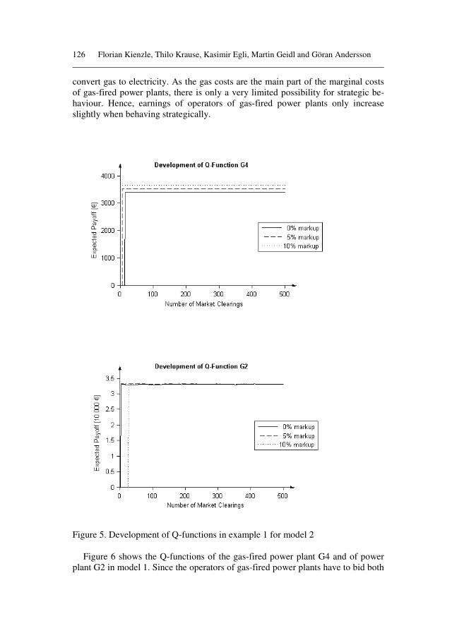
126 Florian Kienzle, Thilo Krause, Kasimir Egli, Martin Geidl and Göran Andersson
convert gas to electricity. As the gas costs are the main part of the marginal costs of gas-fired power plants, there is only a very limited possibility for strategic be-haviour. Hence, earnings of operators of gas-fired power plants only increase slightly when behaving strategically.
Figure 5. Development of Q-functions in example 1 for model 2
Figure 6 shows the Q-functions of the gas-fired power plant G4 and of power plant G2 in model 1. Since the operators of gas-fired power plants have to bid both

Analysis of Strategic Behaviour in Combined Electricity and Gas Markets Using Agent-based Computational Economics 127
in the electricity market and in the gas market, nine different strategies are availa-ble. In the plot at the top of figure 6 (Q-function of G4), the first number in the le-gend is the manipulation of the gas demand bid while the second is the markup for the electricity supply bid.
Figure 6. Development of Q-functions in example 1 for model 1

128 Florian Kienzle, Thilo Krause, Kasimir Egli, Martin Geidl and Göran Andersson
Adding operating costs to the expected gas costs leads to the marginal cost
function. A markup of 10% can be set on these marginal costs. In model 2, opera-tors of gas-fired power plant do not expect a gas price; they simply offer capacity for converting gas to electricity. Hence, they can only set a markup on operating costs without manipulating the gas costs. Since strategic behaviour of the gas-fired power plant in model 2 is much smaller than in the two other models, more energy is traded and hence the ‘total social welfare for electricity production’ (see sub-section 2.2.6) is higher.
Model 1 Model 2 Model 3
φgfpp,opt 0.10 0.10
φgfpp,gas,opt -0.05
φgfpp,op,opt 0.10
Electricity price [€/MWh] 36.97 33.55 37.35
Gas Price [€/MWh] 16.73 17.14 16.69
Pgfpp,el 1220 1591 1178
PL,tot 6220 6591 6179
SW [€] 256’981 257’840 256’787
Table 1. Simulation results for example 1 for every agent choosing its greedy bid after convergence to a stable policy
3.2 Example 2
In example 1, competition between power plants was limited. In example 2, a second gas-fired power plant is added in order to increase competition between gas-fired power plants. Additionally, the line capacities are constraint to investi-gate the behaviour of the models when network topologies are considered. In European electricity markets, transmission losses are usually not taken into ac-count. Losses are therefore neglected in this example, too.
3.2.1 System Data Example 2
The system used in example 2 is similar to the system in example 1 (see figure 3). Unlike in example 1, a second gas-fired power plant (G5) is placed at node 3. Additionally, the capacities of line 2 and line 3 in the electricity network are con-straint to 400 MW. The data for the loads, for the gas supply and for the non-gas-fired power plants are the same as in example 1. Together with the data for the two gas-fired power plants and the PTDF matrix, they are listed in the appendix.

Analysis of Strategic Behaviour in Combined Electricity and Gas Markets Using Agent-based Computational Economics 129
3.2.2 Simulation Results - Example 2
In table 2, the results of the market clearings, where power plants bid according to the strategy with the highest profit expectations, are listed. Since there are con-gested lines in the electricity network, there are different electricity prices at each node.
Model 1 Model 2 Model 3
φgfpp,opt (G4/G5) 0.05 / 0.10 0.05 / 0.10
φgfpp,gas,opt (G4/G5) -0.05 / 0.05
φgfpp,op,opt (G4/G5) 0.10 / 0.00
Electricity price [€/MWh] node 1 35.73 33.84 35.72
Electricity price [€/MWh] node 2 32.42 32.34 32.41
Electricity price [€/MWh] node 3 42.34 42.27 42.33
Gas Price [€/MWh] 17.11 17.24 17.12
Pgfpp,el (G4) [MWh] 631 754 641
Pgfpp,el (G5) [MWh] 1000 1000 1000
PL[MWh] 6300 6353 6301
Pflow [MW] 175 225 181
Pflow [MW] 375 400 378
Pflow [MW] 400 400 400
SW [€] 254’051 254’126 254’055
Table 2. Simulation results for example 2 for every agent choosing its greedy bid after convergence to a stable policy
Since competition between gas-fired power plants in example 2 is increased, it is not very profitable anymore for operators of gas-fired power plants to select high markups. The lowest electricity prices and the highest social welfare for elec-tricity production are still obtained in model 2. Since the highest gas consumption occurs in model 2, the gas price is higher in this case than in model 1 and 3. In dif-ference to example 1, electricity prices and social welfare are nearly the same for model 1 and model 3. This is surprising since in model 3, only the electricity mar-ket is optimised whereas in model 1, overall social welfare of both markets is con-sidered.
4 Conclusions
This paper presented a new modelling approach for combined electricity and gas markets. Two different designs for such combined markets have been pro-posed and analysed in two exemplary cases with regard to the effects on strategic behaviour of market participants. The simulation results of both models have been compared to the outcomes of a market model with separate electricity and gas markets.

130 Florian Kienzle, Thilo Krause, Kasimir Egli, Martin Geidl and Göran Andersson
In example 1, where competition is limited and network constraints are ne-glected, model 2 results in the lowest electricity prices and the highest social wel-fare. The same findings hold true for example 2. The differences between the three models, however, are reduced by increased competition. It has been shown that the good performance of model 2 is mainly due to the fact that gas-fired power plant operators can only manipulate the costs for converting gas to electricity but not the gas costs. In example 2, model 3 surprisingly results in slightly lower elec-tricity prices and higher social welfare than model 1.
Our analysis shows that, under the modelling assumptions we made, combined electricity and gas markets offer potential benefits. In all examples, model 2 re-sults in the highest social welfare and the lowest electricity prices. However, the differences in social welfare are relatively small and it is questionable if this gain in social welfare would justify the expenses for reorganising electricity and natural gas markets. Further and more detailed investigations are therefore needed in or-der to be able to evaluate if the increasing physical coupling between electricity and gas networks can be efficiently assisted by a coupling of the corresponding markets.
Appendix
System data for example 1
The system parameters for loads are shown in table 3 and for non-gas-fired power plants (G1, G2 and G3) in table 5. G1 represents an aggregated hydro units, G2 a nuclear power plant and G3 a conventional thermal power plant. The data for gas supply is listed in table 4. For a gas production of 3000 MW the average gas price at the APX between January 2007 and May 2007 (17.20 €/MWh) is paid. The data for the gas-fired power plant (G4) is listed in table 6.
1
€f
MWh
2 2
€f
MWh
[ ],maxLP MW
L1 79 0.04 1250
L2 99 0.02 3500
L3 99 0.03 2250
Table 3. Load data for the systems used in examples 1 and 2
1
€a
MWh
2 2
€a
MWh
[ ],maxgasP MW
15.40 0.0006 4000
Table 4. Data of the gas supplier for the system used in examples 1 and 2
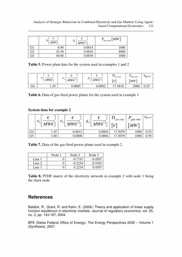
Analysis of Strategic Behaviour in Combined Electricity and Gas Markets Using Agent-based Computational Economics 131
1
€b
MWh
2 2
€b
MWh
[ ],maxgenP MW
G1 6.90 0.0014 1000
G2 24.30 0.0016 4000
G3 40.00 0.0030 1000
Table 5. Power plant data for the system used in examples 1 and 2
1
€e
MWh
2 2
€e
MWh
2 2
€g
MWh
[ ],exp
€
gasΠ
[ ],maxgfppP
MW
ηgas,el
G4 1.45 0.0005 0.0002 17.5818 2000 0.55
Table 6. Data of gas-fired power plants for the system used in example 1
System data for example 2
1
€e
MWh
2 2
€e
MWh
2 2
€g
MWh
[ ],exp
€
gasΠ
[ ],maxgfppP
MW
ηgas,el
G4 1.45 0.0012 0.0004 17.5079 1000 0.55
G5 3.80 0.0008 0.0004 17.5079 1000 0.59
Table 7. Data of the gas-fired power plants used in example 2
Node 1 Node 2 Node 3
Line 1 0 -0.7747 -0.4507
Line 2 0 -0.2254 -0.5493
Line 3 0 0.2254 0.4507
Table 8. PTDF matrix of the electricity network in example 2 with node 1 being the slack node
References
Baldick, R., Grant, R. and Kahn, E. (2004): Theory and application of linear supply function equilibrium in electricity markets. Journal of regulatory economics, vol. 25, no. 2, pp. 143-167, 2004. BFE (Swiss Federal Office of Energy). The Energy Perspectives 2035 – Volume 1 (Synthesis), 2007.

132
Boisseleau, F., Kristiansen, T., Petrov, K. and Veen, W. van der (2004): A supply function equilibrium model with forward contracts – an application to wholesale power markets. In 6th IAEE European conference 2004 – Modelling in energy eco-nomics and policy, Zurich, 2004. Bowmans, I. and Hemmes, K. (2002): Optimising energy systems – hydrogen and distributed generation. In Proc. of 2nd International Symposium on Distributed Gen-eration, Stockholm, Sweden, 2002. Geidl, M. (2007): Integrated modelling and optimisation of multi-carrier energy sys-tems. Diss. ETH No. 17141, ETH Zurich, 2007. Geidl, M., Koeppel, G., Favre-Perrod, P., Kloeckl, B., Andersson, G. and Froehlich, K. (2007): Energy Hubs for the Future. IEEE Power & Energy Magazine, vol. 5, no. 1, 2007. Hobbs, B. (2001): Linear complementary models of Nash-Cournot competition in bilateral and POOLCO power markets. IEEE Transactions on Power Systems, vol. 16, no. 2, pp. 194-202, 2001. Hobbs, B, Metzler, C. and Pang, J.-S. (2000): Strategic gaming analysis for electric power systems: an MPEC approach. IEEE Transactions on Power Systems, vol. 15, no. 2, pp. 638-645, 2000. Kaebling, L. P., Littman, M. L. and Moore, A. W. (1996): Reinforced learning: a sur-vey. Journal of artificial intelligence, vol. 4, pp. 237-285, 1996. Krause, T. (2007): Evaluating congestion management schemes in liberalised elec-tricity markets applying agent-based computational economics. Diss. ETH No. 16928, Eidgenössische Technische Hochschule Zürich, 2007. Metzler, C., Hobbs, B. F. and Pang, J.-S. (1996): Nash-Cournot equilibria in power markets on a linearised DC network with arbitrage: formulations and properties. Networks and spatial economics, vol. 3, pp. 123-285, 1996. Minoia, A., Ernst, D. and Ilic, M. (2004): Market dynamics driven by the decision-making of both power producers and transmission owners. In IEEE PES general meeting, Denver, 2004. NEA, OECD, IEA (2005): Projected cost of generating electricity. Update 2005. Watkins, C. (1989): Learning from delayed rewards. Ph.D. dissertation, Cambridge University, 1989.