D ive rsity a n d D issim ila rity C o e fficie n ts: A U ... · U n ive rsity o f P ittsb u rg h ,...
20
THEORETICAL POPULATION BIOLOGY 21, 24-43 (1982) Diversity and Dissimilarity Coefficients: A Unified Approach ~.RADHAKRISHNA RAO* Institute for Statistics and Applications, Department of Mathematics and Statistics, University of Pittsburgh, Pittsburgh, Pennsylvania I5260 Received September 1. 1980 Three general methods for obtaining measures of diversity within a population and dissimilarity between populations are discussed. One is based on an intrinsic notion of dissimilarity between individuals and others make use of the concepts of entropy and discrimination. The use of a diversity measure in apportionment of diversity between and within populations is discussed. 1. INTRODUCTION There is an extensive literature on measures of diversity within populations and dissimilarity or similarity between populations. They have been used in a wide variety of studies in anthropology (Rao, 1948; Mahalanobis et al., 1949; Majumdar and Rao, 1958; Rao, 1971a,b, 1977), in genetics (Cavalli- Sforza, 1969; Karlin et al., 1979; Morton and Lalovel, 1973; Nei, 1978; Sanghvi, 1953; Sanghvi and Balakrishnan, 1972), in economics (Gini, 1912; Sen, 1973), in sociology (Agresti and Agresti, 1978) and in biology (Sokal and Sneath, 1963; Pielou, 1975; Patil and Taille, 1979). An extensive bibliography of papers on measures of diversity and their applications is compiled by Dennis et al. (1979). Most of these measures are based on heuristic considerations; some are derived from mathematically well-postulated axioms, while others are constructed assuming some models for genetic and environmental mechanisms causing differences between individuals and populations. The object of this paper is to review some of these measures and to provide some unified approaches for deriving them. We consider a set of populations {xi), where the individuals of each population are characterized by a set of measurements XE (Q, -Y?), a * The work of this author is sponsored by the Air Force Offrce of Scientific Research under Contract F49620-79-0161. Reproduction in whole or in part is permitted for any purpose of the United States Government. 24 0040-5809/82/010024-2OSO2.00/0 Copyright ‘0 I982 by Academic Press, Inc. All rights of reproduction in any form reserved.
Transcript of D ive rsity a n d D issim ila rity C o e fficie n ts: A U ... · U n ive rsity o f P ittsb u rg h ,...

THEORETICAL POPULATION BIOLOGY 21, 24-43 (1982)
Diversity and Dissimilarity Coefficients: A Unified Approach
~.RADHAKRISHNA RAO*
Institute for Statistics and Applications, Department of Mathematics and Statistics,
University of Pittsburgh, Pittsburgh, Pennsylvania I5260
Received September 1. 1980
Three general methods for obtaining measures of diversity within a population and dissimilarity between populations are discussed. One is based on an intrinsic notion of dissimilarity between individuals and others make use of the concepts of entropy and discrimination. The use of a diversity measure in apportionment of diversity between and within populations is discussed.
1. INTRODUCTION
There is an extensive literature on measures of diversity within populations and dissimilarity or similarity between populations. They have been used in a wide variety of studies in anthropology (Rao, 1948; Mahalanobis et al., 1949; Majumdar and Rao, 1958; Rao, 1971a,b, 1977), in genetics (Cavalli- Sforza, 1969; Karlin et al., 1979; Morton and Lalovel, 1973; Nei, 1978; Sanghvi, 1953; Sanghvi and Balakrishnan, 1972), in economics (Gini, 1912; Sen, 1973), in sociology (Agresti and Agresti, 1978) and in biology (Sokal and Sneath, 1963; Pielou, 1975; Patil and Taille, 1979). An extensive bibliography of papers on measures of diversity and their applications is compiled by Dennis et al. (1979).
Most of these measures are based on heuristic considerations; some are derived from mathematically well-postulated axioms, while others are constructed assuming some models for genetic and environmental mechanisms causing differences between individuals and populations. The object of this paper is to review some of these measures and to provide some unified approaches for deriving them.
We consider a set of populations {xi), where the individuals of each population are characterized by a set of measurements XE (Q, -Y?), a
* The work of this author is sponsored by the Air Force Offrce of Scientific Research under Contract F49620-79-0161. Reproduction in whole or in part is permitted for any purpose of the United States Government.
24 0040-5809/82/010024-2OSO2.00/0 Copyright ‘0 I982 by Academic Press, Inc. All rights of reproduction in any form reserved.
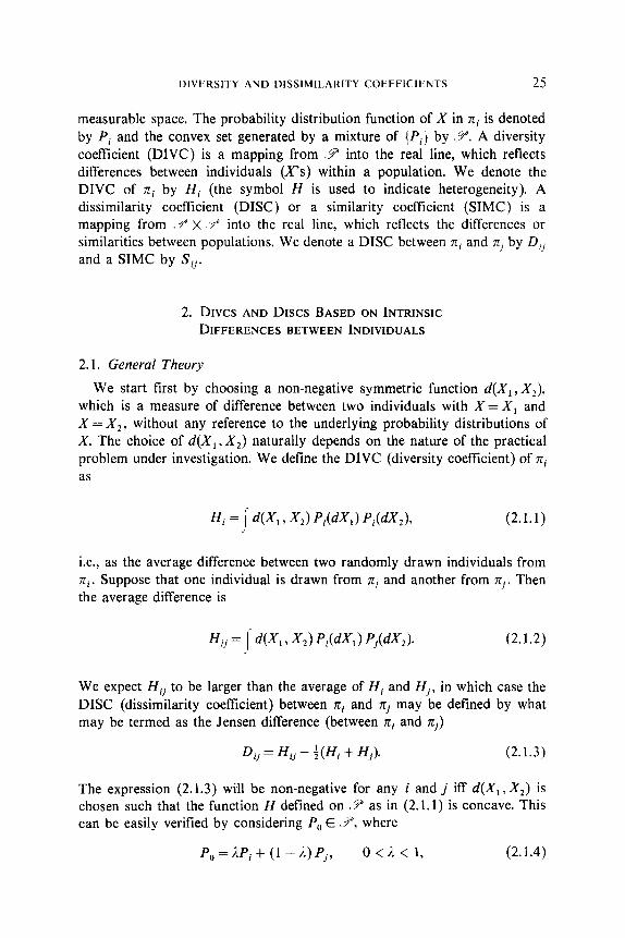
DIVERSITY AND DISSIMILARITY COEFFICIENTS 25
measurable space. The probability distribution function of X in rri is denoted by Pi and the convex set generated by a mixture of {Pi} by 9. A diversity coefficient (DIVC) is a mapping from 9 into the real line, which reflects differences between individuals (X’s) within a population. We denote the DIVC of xi by Hi (the symbol H is used to indicate heterogeneity). A dissimilarity coefficient (DISC) or a similarity coefficient (SIMC) is a mapping from f x .“P into the real line, which reflects the differences or similarities between populations. We denote a DISC between xi and 7cj by Dii and a SIMC by S,.
2. DIVCS AND DISCS BASED ON INTRINSIC DIFFERENCES BETWEEN INDIVIDUALS
2.1. General Theory We start first by choosing a non-negative symmetric function d(X,, X,),
which is a measure of difference between two individuals with X=X, and X = X,, without any reference to the underlying probability distributions of X. The choice of d(X,, X,) naturally depends on the nature of the practical problem under investigation. We define the DIVC (diversity coefficient) of xi as
Hi = - d(Xl 3 x*) pi(dxl) pi(dx*), J (2.1.1)
i.e., as the average difference between two randomly drawn individuals from rci. Suppose that one individual is drawn from zi and another from rrj. Then the average difference is
Hij = I_ d(X, Y x*) Pi(dXl) Pj(dx*). (2.1.2)
We expect H, to be larger than the average of Hi and Hj, in which case the DISC (dissimilarity coefficient) between zi and zj may be defined by what may be termed as the Jensen difference (between ?ri and S)
D, = H, - +(Hi + Hj). (2.1.3)
The expression (2.1.3) will be non-negative for any i and j iff d(X,, X,) is chosen such that the function H defined on P as in (2.1.1) is concave. This can be easily verified by considering P, E ,Y, where
p,=;lpi+ (1 -A)P,, O<L<l, (2.1.4)

26 C. RADHAKRISHNA RAO
and computing
= l*Hi + (1 - A)’ Hj + 2L( 1 - ,I) H,. (2.1.5)
Then
= 24 1 - A)(H, - iHi - +Hj) = 2A( 1 - 1) D,.
The concavity of H ensures that D, > 0 and vice versa.
(2.1.6)
Note 1. In the definition (2.1.1) of diversity no condition is imposed on the function d(X,, X,) except that it should be nonnegative and should have an intrinsic biological meaning. The logical requirement that the Jensen difference (2.1.3) should be nonnegative restricts the choice of d(X, , X2) to functions which induce a concave functional on .P.
Note 2. We may define the expression (2.1.6) involving prior probabilities A and (1 - A) for xi and 7cj as a more general Jensen difference between xi and nj. Fortunately, this difference is only a constant multiple of (2.1.3).
Note 3. The Jensen difference (2.1.3) is a function defined on ,Y X .?. Suppose that we are measuring dissimilarity between say two linguistic groups L, , L, residing in two different cities C, and C, . Let D:, and Dy2 be the DISCS between L, and L, in C, and C,, respectively, and D,, between L, and L, when the populations in the two cities are mixed. In such a case, we expect D,, to be smaller than (D:, + Df,)/2. This logical requirement demands that the Jensen difference (2.1.3) should be a convex function on .Y x P, which imposes a further restriction on the choice of d(X,, X,). Some studies based on the convexity of (2.1.3) have been recently made by Burbea and Rao (1980) and Rao (198 1).
2.2. Some Examples (1) Let X E R”, a real vector space of m dimensions furnished with an
inner product (x, y) = x’Ay, where A is a positive definite matrix. Define
4x1, x2> = (X, - x2 3 x, -x2>. (2.2.1)
Let X- Ni, Zi) in zi (i.e., X is distributed with mean vector pi and dispersion matrix Zi and not necessarily m-variate normal). Then
Hi=2trAZi,
H, = tr AC, + tr AZj + 6;Ahii, (2.2.2)

DIVERSITY AND DISSIMILARITY COEFFICIENTS 27
where tr stands for the trace of a matrix and 6, = ,ui -,uj. Applying the formula (2.1.3)
D, = &Ad,. (2.2.3)
If Zi = C for all i and A = C-l, (2.2.3) becomes the Mahalanobis D* between q and xi.
(2) Let X = (x1 ,..., x,), where xi can take only a finite number of values. For instance, xi may stand for the type of gene allele at a given locus i on a chromosome. In such a case an appropriate measure of difference between two vectors X, and X2 is
d(X,,X,)=m-Cd,, (2.2.4)
where 6, = 1 if the rth components of X, and X, agree and zero otherwise. Let x, take k, different values with probabilities
Girl 1*‘*) Pirk,
in population 7ci. Define
jr’ = E(q) = ; pfr, s=l
when X,, X2 are independently drawn from q and
jp = E(fj,) = 2 Pin Pjrs S=l
when X, is drawn from 7ci and X2 from nj. Then
Hi = 2 (1 -jj;‘) = m(1 -Jii), r=1
(2.2.5)
(2.2.6)
(2.2.7)
H,= 2 (1 -&‘)=m(l -Jij), i-=1
D, = H, - +(Hi + Hj)
= rn[f(Jii + Jjj) - Jij] = 4 2 2 (pirs - pjrsy. r=, s=1
(2.2.8)
The expression (2.2.8) without the factor m has been called by Nei (1978) as “a minimum estimate of the net codon difference per locus” and used by him and his colleagues (see the list of references in Nei, 1978) as a measure of genetic distance in phylogenetic studies.

28 C. RADHAKRISHNA RAO
Note 1. When m = 1, we have a single multinomial and the expression (2.2.8) reduces to the Gini-Simpson index
1 - x Pf, i: 1
(2.2.9)
where p, ,...,pk are the cell probabilities. [This measure was introduced by Gini (1912) and used by Simpson (1949) in biological work.] The properties of (2.2.9) have been studied by various authors (Bhargava and Doyle, 1974; Bhargava and Uppuluri, 1975; Agresti and Agresti, 1978).
Note 2. It is seen that Hi as defined in (2.2.7) depends only on the marginal distributions of xi, i = l,..., m, and is additive with respect to the characters examined. These properties arise from the way the difference function (2.2.4) is defined. The DISC (2.2.8) is specially useful in evolutionary studies as suggested by Nei (1978).
Note 3. We may consider the joint distribution of (x, ,..., x,) as a combined multinomial with k= k, x ..- x k, classes and apply the formula (2.1.1) to measure diversity. In such a case the difference between two individuals takes the value 1 when all the components xi agree and the value zero if at least one is different. This leads to an expression different from (2.2.8), as the basic function for assessing the differences between individuals is not the same. When xi,..., x, are independently distributed, an explicit expression for the DIVC based on the combined multinomial reduces to
H=l-[1-H(l)]...[l-H(m)], (2.2.10)
where H(r) is the DIVC based on x,, the rth character only. It may be noted that the expression for DIVC given in (2.2.7) is H = ZH(r) whether xi are independently distributed or not.
Note 4. If we consider the component x, in the vector X of Note 2 as the genotype of a diploid organism as determined by a pair of allels at locus r and define 6, in (2.2.4) as 1 if two individual organisms have the same value for x, and zero otherwise, then we get the DIVC and DISC based on the measure of genotypic identity devised by Hedrick (1971) and applied by Mitton (1977) in genetic studies. The expressions are the same as in (2.2.5)- (2.2.8) with pirs interpreted as genotype frequencies instead of gene fre- quencies.
Note 5. If we consider x, as a genotype as in Note 4, but define the difference as 2m - Cd,., where 6, is the number of genes common to the individuals at the rth pair of loci (which may be two, one or zero), then we obtain the DIVC and DISC based on a measure introduced by Latter (1973, 1980).
DIVERSITY AND DISSIMILARITY COEFFICIENTS 29
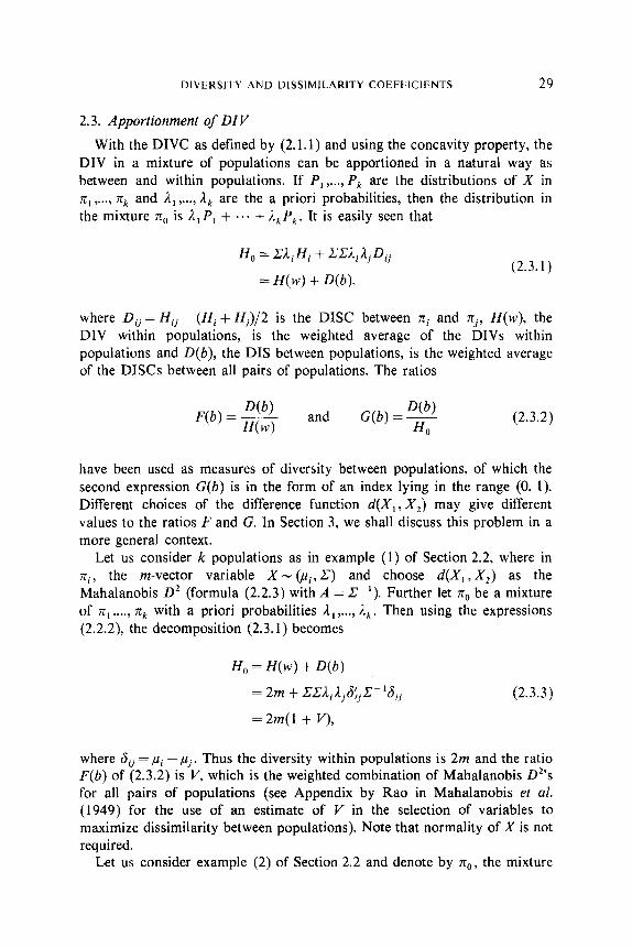
2.3. Apportionment of DIV With the DIVC as defined by (2.1.1) and using the concavity property, the
DIV in a mixture of populations can be apportioned in a natural way as between and within populations. If P, ,..., P, are the distributions of X in n, ,,.., nk and A, ,..., A, are the a priori probabilities, then the distribution in the mixture 7c0 is i, P, + +. . + LkPk. It is easily seen that
H,=~ZiHi + ~;C~i~jDij
= H(w) + D(b), (2.3.1)
where D, = H, - (Hi + Hj)/2 is the DISC between 7~~ and rcj, H(w), the DIV within populations, is the weighted average of the DIVs within populations and D(b), the DIS between populations, is the weighted average of the DISCS between all pairs of populations. The ratios
F(b) = Do H(w)
and G(b) = F 0
(2.3.2)
have been used as measures of diversity between populations, of which the second expression G(b) is in the form of an index lying in the range (0, 1). Different choices of the difference function d(X,, X,) may give different values to the ratios F and G. In Section 3, we shall discuss this problem in a more general context.
Let us consider k populations as in example (1) of Section 2.2, where in 7ci 3 the m-vector variable X- bi, C) and choose d(X,, X,) as the Mahalanobis 0’ (formula (2.2.3) with A = ,I:-‘). Further let no be a mixture of 7c, )...) 7tk with a priori probabilities A,,..., A,. Then using the expressions (2.2.2), the decomposition (2.3.1) becomes
Ho = H(w) + D(b)
= 2m + ZLLiLj&yC-‘6ij (2.3.3)
= 2m(l + V),
where 6, = ,ui - ,LI~. Thus the diversity within populations is 2m and the ratio F(b) of (2.3.2) is V, which is the weighted combination of Mahalanobis D2’s for all pairs of populations (see Appendix by Rao in Mahalanobis et al. (1949) for the use of an estimate of V in the selection of variables to maximize dissimilarity between populations). Note that normality of X is not required.
Let us consider example (2) of Section 2.2 and denote by rc,, the mixture

30 C. RADHAKRISHNA RAO
of x, )...) rrk with a priori probabilities 1, ,..., 1,. In this case (2.3.1) becomes, with Jii as defined in (2.2.7),
H, = m[~Zi( 1 - Jii) + ~~~inj(~Jii + tJjj - Jij)], (2.3.4)
which is the decomposition obtained by Nei (1973) and Chakraborty (1974). The ratio G(b) defined in (2.3.2) is
G(b) = ~~~i~j(~ Jii + fJjj - Jij)
1 - Z&AjJij * (2.3.5)
The ratio (2.3.5) obtained by considering only the with equal prior probabilities
e,,= Jii+Jjj-2Jij ” 4 - Jii - Jjj - 2Jij
two populations xi and 5
(2.3.6)
is the hybridity coefficient of Morton (1973) who used it as a DISC between xi and xj in phylogenetic studies.
2.4. Decomposition of DIVC and DISC In the method outlined in Section 2.1, the basic expression which
determines the DIVC and DISC is the difference function d(X,, X,). Any decomposition of d(X,, X,) such as
4X,, X,) = 4(X,, X,) + ... + 4(X,, X,) (2.4.1)
provides us with a corresponding decomposition of the DIVC for rri
H.=jq” + . . . I +@C’ > (2.4.2)
where HI”’ = E [ d,(X, , X,) 1 Pi], and of the DISC between xi and rcj
D.,z D!!’ + . . . + D(f) IJ lJ I, ’ (2.4.3)
where 0::’ is obtained from Hi , O) H,(” and Hi;’ using the formula (2.1.3). Let X - (ui, Z) in xi and denote the eigenvalues of C by 8, > . .. > 8, and
the corresponding normalized orthogonal eigenvectors by L, ,..., L,. If we choose
4X,, X,> = (X, - X,>‘(X, - X,), i.e., the simple Euclidean distance in Rm, then
d(X,, X,) = [L:(X, -X,)]’ + a.4 + (L’,(X, -X,)1’ (2.4.4)

DIVERSITY AND DISSIMILARITY COEFFICIENTS 31
gives the decomposition of DIVC for ni
Hi=2trC=28,+a.. t28,, (2.4.5)
which is the familiar decomposition of total variability with respect to m characters in terms of principal components (Rao, 1964). The corresponding decomposition of DISC between xi and xj is
Dij = 6:,6, = (L; 6,)2 + *. . $ (L:, S,)‘, (2.4.6)
where 6, = ,U~ - ,uj, the difference in the mean vectors for 7ci and ?ri. However. if we choose
i.e., the Mahalanobis distance between two individuals then we have a different decomposition
D, = s;a?- ‘8, = $ (L; 6,)’ + ‘*. t + (L:,Sij)2. (2.4.6) I m
Note that the eigen vectors provide a transformation of the original measurements into uncorrelated variables, in which case the Mahalanobis distance can be written as the sum of Mahalanobis distances due to different uncorrelated variables. We can choose any arbitrary set of vectors M ,,..., M, such that M:CMj= 0 for i #j and MiZMi = 1, to obtain a decomposition
D, = S;~- ‘6, = (M’, S,)’ + . . . + (M:, S,)’
= D!!’ f . . . + D(m) (2.4.7)
IJ 1J ’
By combining some of the Dijs on the right-hand side of (2.4.7), we obtain decompositions of D, with a smaller number of components.
If we choose
M, = (CAT-‘o)- v2 C-b (2.4.8)
in (2.4.7), where cr is the vector of standard deviations of the individual characters (i.e., square roots of diagonal elements of C), then
(M; aij)* = Dzi (2.4.9)
represents the component of Mahalanobis D2 between ni and 7cj due to the size factor as defined by Rao (1962, 197 1 b). Then
Dij=D2=DfifD$,, (2.4.10)

32 C. RADHAKRISHNA RAO
where D:,,, the residual after subtracting the D* due to size, represents the distance due to shape factors between the two populations.
Penrose (1954) obtained a similar decomposition of Karl Pearson’s CRL (coefficient of racial likeness) in terms of size and shape. The Penrose indices do not take into account the correlations that may exist between characters. For further details regarding the use of size and particular shape factors reference may be made to Rao (1962, 197 lb).
2.5. Similarity Coeficients (SIMCs) Instead of a difference measure between two individuals, it may be natural
to consider a similarity function s(X,, X,) and define Si, Sj and S, by taking expectations analogous to Hi, Hj and H,. Then the DIVC of q may be defined by a suitable decreasing function of Si, such as 1 - Si or -log Si, specially when the range of Si is (0, 1). The DISC obtained by choosing Hi = 1 - Si, provided it satisfies the concavity condition, is
D, = +(Si + Sj) - S,
and that by choosing Hi = -log Si is
D, = ;(log Si + log Sj) - log S,
= -log &,
(2.5.1)
(2.5.2)
For instance, in the second example of Section 2.2, a natural definition of SVl~ X2) = (W/ m, which lies in the range (0, 1). Then
Si = Jii, Sj= Jjj, S, = Jij, (2.5.3)
where J, are as defined in (2.2.7), and using (2.5.1) and (2.5.2) we have the alternative forms
D, = ;(Jii + Jjj) - Jij, (2.5.4)
(2.5.5)
The expression (2.5.4) is the same as the “minimum genetic distance” (2.2.8) of Nei (1978), and (2.5.5) is what he calls the “standard genetic distance.”
Again, in the example (2), we may define the similarity function as (6, **- Smym instead of (6, + ..a + 6,)/m. The new function has the value unity when the gene alleles coincide at all the loci and zero otherwise. In such a case, when the characters are independent,

DIVERSITY AND DISSIMILARITY COEFFICIENTS 33
(2.5.6)
where j:J’ are as defined in (2.2.5) and (2.2.6). Taking logarithms of (2.5.6) the corresponding DISC is
(2.5.7)
which Nei calls the “maximum genetic distance.” Since Si + Sj > 2S,, we may define an index of similarity 2S,/(S, + Sj)
as proposed by Hedrick (1971). This lies in the range (0, 1) and the corresponding DISC may be defined as
2s.. D, = -log 2 Si + Sj
(2.5.8)
which is analogous to (2.5.7).
3. ENTROPY AND INFORMATION
3.1. Measures of Entropy A wide variety of DIVCs have been introduced through the concept of
entropy and information. The general approach in these cases is basically different from that of Section 2.1, where a function d(X,, X,) measuring the difference between individuals X, and X, is chosen first and probability distributions of Xi and X, are used only to find the average of d(X,, X,). In practice, d(X,, X,) would be chosen to reflect some intrinsic dissimilarity between individuals relevant to a particular investigation. On the other hand, a measure of entropy is directly conceived of as a function defined on the space of distribution functions, satisfying some postulates. Some of the postulates are that it is non-negative, attains the maximum for the uniform distribution and has the minimum when the distribution is degenerate. Thus a measure of entropy is an index of similarity of a distribution function with the uniform distribution, and hence a measure of DIV.
We shall consider the space of all multinomial distributions for simplicity of presentation of results, observing that the formulae for the continuous case can be obtained by replacing the summation by the integral sign. We represent the probabilities in the k cells of a general multinomial by pI ,..., pk and for a particular population 7zi by pi1 ,...,pik. Mathai and Rathie (1975) consider three general forms for entropy:
34 C. RADHAKRISHNA RAO
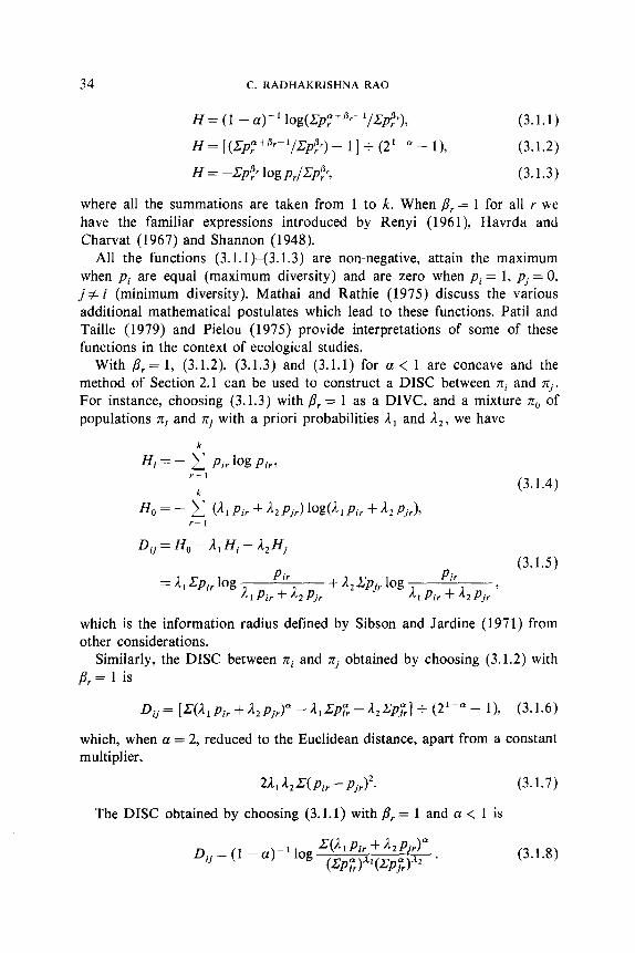
H = (1 - a) - ’ lo&L”; + 4r- ‘/.Z”;$ (3.1.1)
H = [(Zpr”+br-l/Zp~r) - I] t (21Pn - l), (3.1.2)
H = -Cpfr log p,/Zp$, (3.1.3)
where all the summations are taken from 1 to k. When /I, = 1 for all r we have the familiar expressions introduced by Renyi (1961), Havrda and Charvat (1967) and Shannon (1948).
All the functions (3.1.1)-(3.1.3) are non-negative, attain the maximum when pi are equal (maximum diversity) and are zero when pi = 1, pj = 0, j # i (minimum diversity). Mathai and Rathie (1975) discuss the various additional mathematical postulates which lead to these functions. Patil and Taille (1979) and Pielou (1975) provide interpretations of some of these functions in the context of ecological studies.
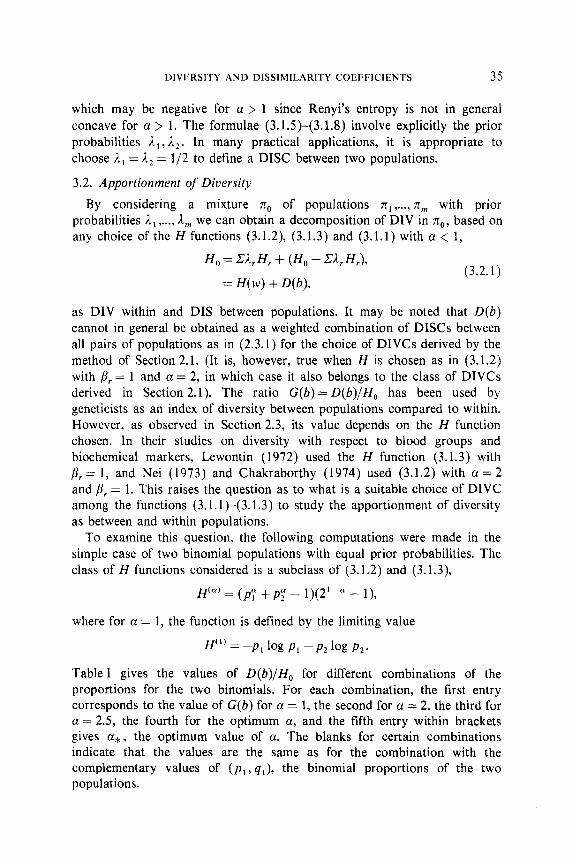
With /3, = 1, (3.1.2) (3.1.3) and (3.1.1) for (x < 1 are concave and the method of Section 2.1 can be used to construct a DISC between 7ci and ~j. For instance, choosing (3.1.3) with p, = 1 as a DIVC, and a mixture 7~~ of populations 7ci and rcj with a priori probabilities L, and A,, we have
Hi = - ~ pir log Pir, r= 1
Ho=- f’ (~,Pir+~,Pj,)log(~,Pi,+~2Pj,),
(3.1.4)
r=1
D, = H,, - 1, Hi - 12 Hj
= 1, zpi, log Pir pjr (3.1.5)
I1 Pir + l2 Pjr + n,.gpj, log
AlPir+A2Pjr’
which is the information radius defined by Sibson and Jardine (1971) from other considerations.
Similarly, the DISC between rci and rcj obtained by choosing (3.1.2) with p, = 1 is
D,= [.Z(A,p, + A,pj,)” - A,Zp: -A,Ep;] f (21--a - l), (3.1.6)
which, when a = 2, reduced to the Euclidean distance, apart from a constant multiplier,
2Aln2c(Pir -Pjr)‘. (3.1.7)
The DISC obtained by choosing (3.1.1) with p,. = 1 and a < 1 is
(3.1.8)
DIVERSITY AND DISSIMILARITY COEFFICIENTS 35
which may be negative for a > 1 since Renyi’s entropy is not in general concave for a > 1. The formulae (3.1.5~(3.1.8) involve explicitly the prior probabilities A,, A,. In many practical applications, it is appropriate to choose AI = I, = l/2 to define a DISC between two populations.
3.2. Apportionment of Diversity By considering a mixture 7t0 of populations x,,..., 71, with prior
probabilities A, ,..., Am we can obtain a decomposition of DIV in 7c,,, based on any choice of the H functions (3.1.2), (3.1.3) and (3.1.1) with a < 1,
H, = CL,. H, + (H, - Z&H,),
= H(w) + D(b), (3.2.1)
as DIV within and DIS between populations. It may be noted that D(b) cannot in general be obtained as a weighted combination of DISCS between all pairs of populations as in (2.3.1) for the choice of DIVCs derived by the method of Section 2.1. (It is, however, true when H is chosen as in (3.1.2) with /?, = 1 and a = 2, in which case it also belongs to the class of DIVCs derived in Section 2.1). The ratio G(b) = D(b)/HO has been used by geneticists as an index of diversity between populations compared to within. However, as observed in Section 2.3, its value depends on the H function chosen. In their studies on diversity with respect to blood groups and biochemical markers, Lewontin (1972) used the H function (3.1.3) with p,= 1, and Nei (1973) and Chakraborthy (1974) used (3.1.2) with a = 2 and /3, = 1. This raises the question as to what is a suitable choice of DIVC among the functions (3.1.1~(3.1.3) to study the apportionment of diversity as between and within populations.
To examine this question, the following computations were made in the simple case of two binomial populations with equal prior probabilities. The class of H functions considered is a subclass of (3.1.2) and (3.1.3),
Hca’ = (py +p; - 1)(2’-* - l),
where for a = 1, the function is defined by the limiting value
H’“=-p,logp,-pp,logp,.
Table I gives the values of D(b)/H,, f or different combinations of the proportions for the two binomials. For each combination, the first entry corresponds to the value of G(b) for a = 1, the second for a = 2, the third for a = 2.5, the fourth for the optimum a, and the fifth entry within brackets gives a*, the optimum value of a. The blanks for certain combinations indicate that the values are the same as for the combination with the complementary values of (pl, ql), the binomial proportions of the two populations.
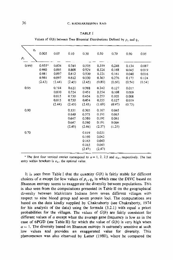
36 C. RADHAKRISHNA RAO
TABLE I
Values of G(b) between Two Binomial Distributions Defined by pI and q1
0.995 0.955* 0.834 0.980 0.895 0.981 0.897 0.98 I 0.897 (2.43) (2.44)
0.714 0.810 0.815 0.815 (2.44)
0.95
0.90
0.70
0.10 0.30 0.50 0.70 0.90 0.95
0.741 0.808 0.812 0.812 (2.45)
0.622 0.724 0.730 0.730 (2.45)
0.53 I 0.640 0.647 0.647 (2.45)
0.505 0.529 0.530 0.530 (2.45)
0.388 0.45 1 0.454 0.454 (2.45)
0.305 0.375 0.380 0.380 (2.46)
0.119 0.160 0.163 0.163 (2.47)
0.359 0.248 0.324 0.168 0.321 0.161 0.363 0.276 (0.80) (0.60)
0.242 0.127 0.254 0.108 0.253 0.105 0.255 0.127 (1.69) (0.97)
0.167 0.065 0.191 0.063 0.191 0.06 1 0.191 0.066 (2.37) (1.25)
0.03 1 0.042 0.043 0.043 (2.47)
0.134 0.087 0.045 0.019 0.040 0.016 0.173 0.124 (0.54) (0.54)
0.017 0.009 0.008 0.019 (0.73)
* The first four vertical entries correspond to a = 1, 2, 2.5 and a,, respectively. The last entry within brackets is (I*, the optimal value.
It is seen from Table I that the quantity G(b) is fairly stable for different choices of a except for low values of pi, q, in which case the DIVC based on Shannon entropy seems to exaggerate the diversity between populations. This is also seen from the computations presented in Table II on the geographical diversity between Makiritare Indians from seven different villages with respect to nine blood group and seven protein loci. The computations are based on the data kindly supplied by Chakraborty (see Chakraborty, 1974 for his analysis of the data) using the formula (3.2.1) with equal a priori probabilities for the villages. The values of G(b) are fairly consistent for different values of a except when the average gene frequency is low as in the case of 6PGD (see Table II) for which the value of G(b) is very high when CT = 1. The diversity based on Shannon entropy is extremely sensitive at such low values and provides an exaggerated value for diversity, This phenomenon was also observed by Latter (1980), where he compared the

DIVERSITY AND DISSIMILARITY COEFFICIENTS 31
TABLE II
Gene DIV of Makiritare Indians in Seven Villages and Index of DIS between Villages
LQCUS
a=1 a=2 a = 2.5 Ave
P HO G(b) Ho G(b) 4 WI
Serological Diego Kidd WC) P Lewis SS WE) MN Duffy
0.196 0.7139 0.1743 0.6303 0.1711 0.6240 0.1693 0.336 0.9209 0.0250 0.8924 0.0320 0.8899 0.0325 0.418 0.9805 0.040 1 0.9731 0.0542 0.9724 0.0554 0.434 0.9874 0.0172 0.9826 0.0232 0.9821 0.0237 0.466 0.9967 0.0791 0.9954 0.1044 0.9952 0.1191 0.470 0.9974 0.0575 0.9964 0.0770 0.9963 0.0786 0.563 0.9885 0.0058 0.9841 0.0079 0.9837 0.008 1 0.714 0.8635 0.0263 0.8168 0.029 1 0.8128 0.0292 0.736 0.8327 0.0122 0.7772 0.0142 0.7726 0.0166
Average 0.9202 0.0415 0.8943 0.0448 0.8921 0.0486
Biochemical AP HP Gc PGM, LP Alb 6PGD
0.0557 0.3101 0.0647 0.2104 0.0238 0.2054 0.0213 0.424 0.9833 0.0650 0.9769 0.0866 0.9763 0.0884 0.820 0.6801 0.043 1 0.5904 0.0432 0.5837 0.0427 0.848 0.6148 0.0592 0.5156 0.0504 0.5086 0.0488 0.876 0.5407 0.0084 0.4345 0.0052 0.4275 0.0047 0.9857 0.1081 0.1293 0.0564 0.1719 ( 0.0547 0.1444 0.991 0.0741 0.2503 0.0357 0.0678 0.0346 0.0934
Average 0.4730 0.0561 0.4028 0.0521 0.3987 0.0522
performance of diversity coefficients based on the Shannon entropy, Hedrick’s measure of genotype identity and Latter’s measure of gene identity. Based on these studies and Latter’s observation that “Shannon’s measure of information... has many convenient properties from a mathematical point of view, but is extremely difficult to interpret genetically,” it appears that the DIVC based on Shannon’s entropy is at a disadvantage compared to the others.
4. DISCRIMINATION INDEX
A general method of constructing DISCS is through the concept of discrimination between populations, i.e., the probability with which a given

38 C. RADHAKRISHNA RAO
individual can be identified as a member of one of two populations to which he possibly belongs.
4.1. Overlap Distance (Rao, 1948, 1977; Wald, 1950)
Let X be a set of measurements which has the probability density pi(.) in 7ci and pi(a) in rrj. The best decision rule based on an observed value x of X, for discriminating between xi and rrj with prior probabilities in the ratio 1 : 1 is to assign x to
population rci if PiCx) > PjCx>Y (4.1.1)
population 7ti if Pitx> < PjCx>3
and to decide by tossing an unbiased coin when pi(x) =pj(x). The probability of correct classifications for the optimum decision rule is
C, = f 1 pi(X) dx + 4 1 pj(x) dx, (4.1.2) RI R2
where R, is the region pi(x) >pj(x) and R,, the region pj(x) > p,(x). The minimum value of (4.2) is l/2 which is attained when p,(a) =~](a), and the maximum is unity when the supports of pi(.) and pj( .) are disjoint. The more dissimilar the populations are, the greater would be the probability of correct classifications. Then we may define the DISC between zi and rrj as
D, = C, - ), (4.1.3)
which is in the range (0, f). It is seen that
cij -; = + i lpi(X) -pi(X)1 dx, (4.1.4)
which is a multiple of Kolmogorov’s variational distance or city block distance, which is a special case of the Minkowski distance
[I 1 1/t I Pi(X) -Pj(X)l’ dx 3 t> 1. (4.1.5)
In the development of decision theory, Wald (1950) introduced the distance function between rri and rrj,
D, = max 1 Pi(x) - Pj(X> 1 dx y (4.1.6) R

DIVERSITY AND DISSIMILARITY COEFFICIENTS 39
where R represents any arbitrary region. The expression (4.1.6) is iden- tifiable as
D, = 1 - I
min[ pi(x), pi(x)] dx (4.1.7)
= [Pi(x) -Pj(X)] dx, J RI (4.1.8)
where R, is the region p,(x) >pj(x) as in (4.1.2). The expression (4.1.8) is the difference between the proportions of correct and wrong classifications by using the optimum decision rule (4.1.1). The expression (4.1.7) may be interpreted as the proportion of mismatched individuals in the two populations.
4.2. Quadratic Differential Metric (Rao, 1948) Let us consider a family of probability densities p(x, O), 0 E 0, a k-vector
parameter space. The Fisher information matrix at 0 is M= [mij(B)], where
mij(@ = L dp dp dx. J p de, dej (4.2.1)
We endow the space 0 with the quadratic differential metric
LZm,(0) 68, &lj, (4.2.2)
and define the distance between two points 8, and 0, as the geodesic distance determined by (4.2.2). The expression (4.2.2) is a measure of difference between two probability distributions close to each other and the distance defined by it may be useful in evolutionary studies where gradual changes take place in a population in moving from state Or to state 8,. In a recent paper Atkinson and Mitchell (198 1) have derived the expressions for geodesic distances based on (4.2.2) for well-known families of distributions.
4.3. Invariants of Jeffreys Jeffreys (1948) defined what are called invariants between two
distributions
I,= /[Pi(X)]““- [Pj(x)]“m/mdX~ 1 m > 0, (4.3.1)
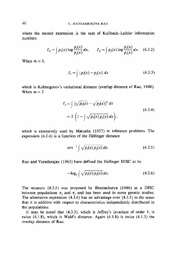
40 C. RADHAKRISHNA RAO
where the second expression is the sum of Kullback-Leibler information numbers
Iij =Jpi(X) log $$ dx, Iji = lpi(X) log ‘g dx. (4.3.2) 3 I
When m = 1,
11~ I I Pi(X) --Pj(x>l dx (4.3.3)
which is Kolmogorov’s variational distance (overlap distance of Rao, 1948). When m = 2
I,= hhi@-di$?l*dx I
=2 l- ( J’ d&f%$%x , 1
(4.3.4)
which is extensively used by Matusita (1957) in inference problems. The expression (4.3.4) is a function of the Hellinger distance
cq l.hmFw. (4.3.5)
Rao and Varadarajan (1963) have defined the Hellinger DISC to be
-log, 1 v’m dx. (4.3.6)
The measure (4.3.5) was proposed by Bhattacharya (1946) as a DISC between populations rci and rrj and has been used in some genetic studies. The alternative expression (4.3.6) has an advantage over (4.3.5) in the sense that it is additive with respect to characteristics independently distributed in the populations.
It may be noted that (4.3.3), which is Jeffrey’s invariant of order 1, is twice (4.1.8) which is Wald’s distance. Again (4.1.8) is twice (4.1.3) the overlap distance of Rao.

DIVERSITY AND DISSIMILARITY COEFFICIENTS 41
5. SOME REMARKS
The paper discusses three unified methods of deriving measures of diversity and dissimilarity. Of these, the new method based on an intrinsic difference between individuals discussed in Section 2 offers a wide scope. The choice of the basic difference function has to be made on biological considerations depending on the problem under investigation. The discrimination approach of Section 4 also admits practical interpretation and the measures based on this approach are specially useful in the study of infraspecilic variation among taxonomical units (Jardine and Sibson, 1971, p. 33). The measures based on the concept of entropy considered in Section 3 have attractive mathematical properties but are difficult to interpret genetically (Latter, 1980).
For the apportionment of genetic diversity between and within populations, a number of diversity measures have been proposed by different authors (see Latter, 1980, Lewontin, 1972 and Nei, 1973). Among those studied, the differences in the estimates of G(b), the index of between population diversity, are of a small order except in the case of Shannon entropy (first used by Lewontin) which seems to give an exaggerated value for diversity between populations when the gene frequencies are at very low levels. Further work is needed to bring out finer distinctions among the other measures.
There has been considerable debate on the choice of a dissimilarity measure in comparing populations. The problem cannot be answered without a reasonably precise statement of the objectives as observed by Smith (1977). If only a descriptive classification of the populations is intended through dendograms or other clustering methods, a fairly large class of measures may lead to the same conclusions. In such cases, it may be useful to try more than one possible measure to test the consistency of final conclusions (see Karlin et al., 1979). In some situations a choice can be made among a number of measures for particular applications, by first testing them on a group of populations whose interrelationships have been otherwise well established. That measure which gives results most consistent with available knowledge may be chosen. Such a procedure has been proposed by Pielou (1979) and applied in choosing one out of nine possible similarity measures in a study on the interpretation of paleoecological similarity matrices. In genetic studies, it is of some importance that the distance function should reflect in an easily interpretable way the basic genetic differences. In such a case the results may have some evolutionary significance (see Morton, 1973 and Nei, 1978). Further theoretical and empirical investigations are necessary to obtain more insight into these problems.

42 C.RADHAKRISHNA RAO
REFERENCES
AGRESTI, A. AND AGRESTI, B. F. 1978. Statistical analysis of qualitative variation, in ‘Social Methodology” (K. F. Schussler, Ed.), pp. 204-237.
ATKINSON, C. AND MITCHELL, A. F. S. 1981. Rao’s distance measure, Sankhya, in press. BHARGAVA, T. N. AND DOYLE, P. H. 1974. A geometric study of diversity, J. Theoret. Bid.
43, 241-25 1. BHARGAVA, T. N. AND UPPULURI, V. R. R. 1975. On diversity in human ecology, Metron 34,
1-13. BHATTACHARYA, A. 1946. A measure of divergence between two multinomial populations,
Sankhya 7, 401. BURBEA, J. AND RAO, C. R. 1980. “On the Convexity of Jensen Difference Arising from
Entropy of Order,” Tech. Report, University of Pittsburgh. CAVALLI-SFORZA, L. L. AND EDWARDS, A. W. F. 1967. Phylogenetic analysis: Models and
estimation procedures, Amer. J. Hum. Genet. 19, 233-257. CAVALLI-SFORZA, L. L. 1969. Human diversity, in “Proceddings, XII Internat. Congr.
Genetics, Tokyo,” Vol. 3, pp. 405416. CHAKRABORTY, R. 1974. A note on Nei’s measure of gene diversity in a substructural popula-
tion, Humangenetik 21, 85-88. DENNIS, B., PATIL, G. P.. Rossr. O., STEHMAN, S.. AND TAILLE, C. 1979. A bibliography of
literature on ecological diversity and related methodology, in “Ecological Diversity in Theory and Practice,” Vol. 1 CPH, pp. 319-354.
GINI, C. 1912. “Variabiliti e Mutabiliti,” Studi Economicoaguridici della facotta di Giurisprudenza dell, Universite di Cagliari III, Parte II.
HAVRADA, J. AND CHARVAT. F. 1967. Quantification method in classification processes: Con- cept of structural a-entropy, Kybernetika 3, 3&35.
HEDRICK, P. W. 1971. A new approach to measuring genetic similarity, Ecoluiion 25. 276-280.
JARDINE, N. AND GIBSON, R. 1971. “Mathematical Taxonomy,” Wiley, New York. JEFFREYS, H. 1948. “Theory of Probability,” 2nd edition. Oxford Univ. Press (Clarendon),
London. KARLIN, S., KENETT, R., AND BONNE-TAMIR, B. 1979. Analysis of biochemical genetic data
on Jewish populations. II. Results and interpretations of heterogeneity indices and distance measures with respect to standards, Amer. J. Hum. Genef. 31, 341-365.
LATTER, B. D. H. 1973. Measures of genetic distance between individuals and populations, in “Genetic Structure of Populations” (N. E. Morton, Ed.) pp. 27-39, Univ. of Hawaii Press, Honolulu.
LATTER, B. D. H. 1980. Genetic differences within and between populations of the major human subgroups, Amer. Natur. 16, 226237.
LEWONTIN, R. C. 1972. The apportionment of human diversity, Evolutionary Biol. 6, 381-398.
MAHALANOBIS, P. C., MAJUMDAR, D. N., AND RAO, C. R. 1949. Anthropometric survey of the United Provinces, 1941: A statistical study, Sankhya 9, 90-324.
MAJUMDAR, D. N. AND RAO, C. R. 1958. Bengal anthropometric survey, 1945: A statistical study. Sankhya 19, 203-408.
MATHAI A. AND RATHIE, P. N. 1974. “Basic Concepts in Information Theory and Statistics,” Wiley (Halsted Press), New York.
MATUSITA, K. 1957. Decision rule based on the distance for the classification problem, Ann. Ins~. Statist. Math. 8, 67-77.
MITTON, J. 1977. Genetic differentiation of races of man as judged by single locus and mul- tilocus analysis. Amer. Natur. 111, 203-2 12.
DIVERSITY AND DISSIMILARITY COEFFICIENTS 43
MORTON, N. E. AND LALOVEL, J. M. 1973. Typology of kinship in Micronesia, Amer. J. Hum. Genet. 25, 422-432.
MORTON, N. E. (1973). Kinship and population structure, in “Genetic Structure of Popula- tions” (N. E. Morton, Ed.), pp. 66-71, Univ. of Hawaii Press, Honolulu.
NEI, M. 1973. Analysis of gene diversity in subdivided populations, Proc. Nat. Acad. Sci. 70, 3321-3323.
NEI, M. 1978. The theory of genetic distance and evolution of human races, Japan. 1. Human Genet. 23, 341-369.
PATIL, G. P. AND TAILLE, C. 1979. An overview of diversity, in “Ecological Diversity in Theory and Practice,” Vol. I CPH, pp. 3-28.
PENROSE, L. S. 1954. Distance, size and shape, Ann. Eugen. 18, 337-343. PIELOU, E. C. 1975. “Ecological Diversity,” Wiley, New York. PIELOU, E. C. 1979. Interpretation of paleoecological similarity matrices, Paleobiology 5,
435443. RAO, C. R. 1945. Information and accuracy attainable in the estimation of parameters, Bull.
Calcutta Math. Sot. 37, 81-91. RAO, C. R. 1948. The utilization of multiple measurements in problems of biological
classification, J. Roy. Statist. Sot. B 13, 159-193. RAO, C. R. 1954. On the use and interpretation of distance functions in statistics, Bull.
Internat. Statist. Inst. 34, 90. RAO, C. R. 1962. Use of discriminant and allied functions in multivariate analysis, Sankhya
A 24, 1499154. RAO, C. R. 1964. The use and interpretation of principal components in applied research,
Sankhya A 26, 329-358. RAO, C. R. 1965, 1973. “Linear Statistical Inference and its Applications,” Wiley, New York. RAO, C. R. 197 la. “Advanced Statistical Methods in Biometric Research,” Haffner (first edi-
tion 1952), Wiley, New York, RAO, C. R. 197 lb. Taxonomy in anthropology, in “Mathematics in the Archaeological and
Historical Sciences,” pp. 19-20, Ed’ b m urgh Univ. Press, Edinburgh. RAO, C. R. 1977. Cluster analysis applied to a study of race mixture in human populations, in
“Proceedings, Michigan Univ. Symp.,” pp. 175-197. RAO, C. R. 1981. “Analysis of Diversity: A Unified Approach,” Univ. of Pittsburgh. Tech.
Rept. 8 l-20. RENYI, A. 1961. On measures of entropy and information, in “Proceedings, Fourth Berkeley
Symp.,” Vol. 1, pp. 547-561. SANGHVI, L. D. 1953. Comparison of genetic and morphological methods for a study of
biological differences, Amer. J. Phys. Anthropol. 11, 385404. SANGHVI, L. D. AND BALAKRISHNAN, V. 1972. Comparison of different measures of genetic
distance between human populations, in “The Assessment of Population Affinities in Man” (J. S. Weiner and J. Huizinga, Eds.), pp. 25-36, Oxford Univ. Press, London.
SEN. A. 1973. “On Economic Inequality,” Oxford Univ. Press (Clarendon), London. SHANNON, C. E. 1948. A mathematical theory of communications, Bell System Tech. J. 27,
379-423, 623-656. SIMPSON, E. H. 1949. Measurement of diversity, Nature 163, 688. SMITH, C. A. B. 1977. A note on genetic distance, Ann. Hum. Genet. (London) 40, 463-479. SOKAL, R. R. AND SNEATH, P. H. A. 1963. “Principles of Numerical Taxonomy,” Freeman,
San Francisco, WALD, A. 1950. “Statistical Decision Functions,” Wiley, New York.