OOIILL WWEELLLL IINNVVEESSTTMMEENNTT SSTTRRAATTEEGGYY

GGRROOUUPP DDEESSIIGGNN PPRROOJJEECCTT

West Virginia UniversityPetroleum & Natural Gas Engineering

Fall 1999PNGE 241: Oil & Gas Property Evaluation

Shahab Mohaghegh, Ph.D.

DDEECCEEMMBBEERR 66,, 11999999

MMUUTTLLAAQQ AALLQQEEMMLLAASSSSTTEEVVEE AAUUJJAAYY

CCAARRRRIIEE GGOODDDDAARRDD

11

EEXXEECCUUTTIIVVEE SSUUMMMMAARRYY

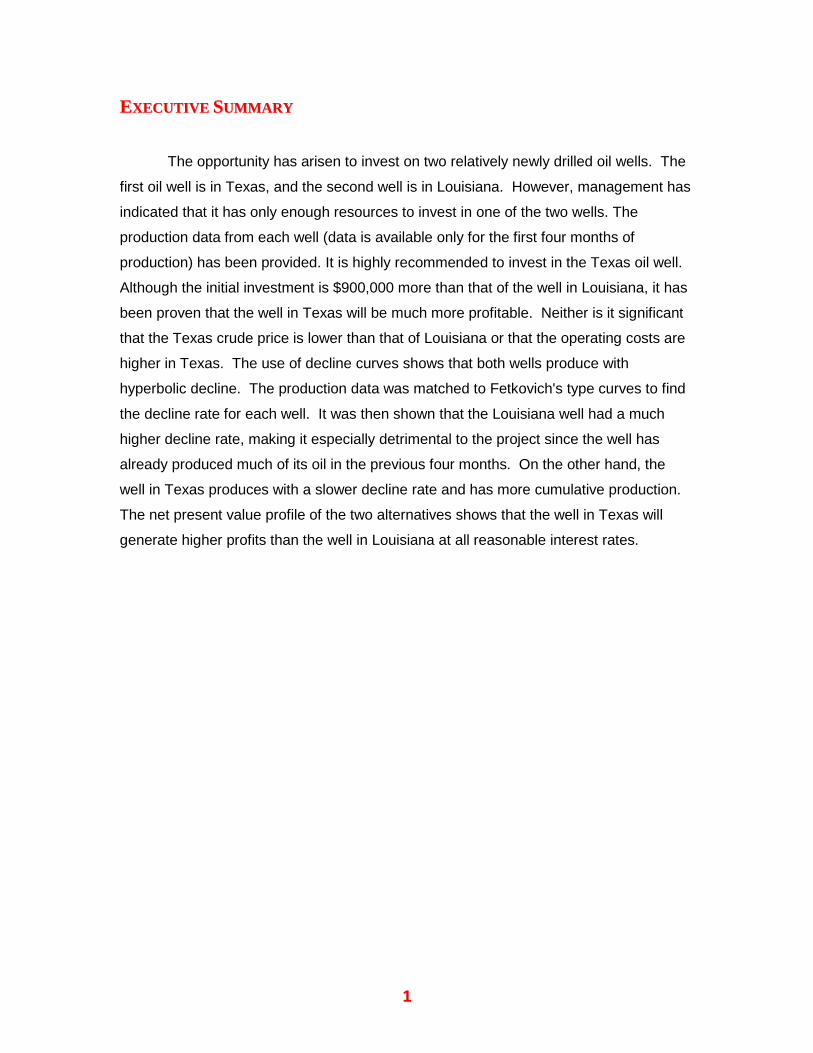
The opportunity has arisen to invest on two relatively newly drilled oil wells. The

first oil well is in Texas, and the second well is in Louisiana. However, management has

indicated that it has only enough resources to invest in one of the two wells. The

production data from each well (data is available only for the first four months of

production) has been provided. It is highly recommended to invest in the Texas oil well.

Although the initial investment is $900,000 more than that of the well in Louisiana, it has

been proven that the well in Texas will be much more profitable. Neither is it significant

that the Texas crude price is lower than that of Louisiana or that the operating costs are

higher in Texas. The use of decline curves shows that both wells produce with

hyperbolic decline. The production data was matched to Fetkovich's type curves to find

the decline rate for each well. It was then shown that the Louisiana well had a much

higher decline rate, making it especially detrimental to the project since the well has

already produced much of its oil in the previous four months. On the other hand, the

well in Texas produces with a slower decline rate and has more cumulative production.

The net present value profile of the two alternatives shows that the well in Texas will

generate higher profits than the well in Louisiana at all reasonable interest rates.

22

PPRROOBBLLEEMM SSTTAATTEEMMEENNTT

The company has been offered to invest on two relatively newly drilled oil wells.

The first oil well is in Texas, and the second well is in Louisiana. Management has

indicated that it has only enough resources to invest in one of the two wells. Therefore,

a recommendation must be made to management on this investment opportunity. The

production data from each well (data is available only for the first four months of

production) has been provided. It is also important to note that the time value of money

for the company over the next three years is 15.5 percent.

Decline curve analysis should be performed using the given production data and

a (monthly) net cash flow for the next three years should be generated for both wells.

Then, the projects may be evaluated with an accredited yardstick, either the discounted

cash flow rate of return technique or the net present value profile. At the conclusion of

the analysis, a recommendation, justified by sound engineering, must be made to

management.

The crude being produced from these two wells are different in quality. The

crude from Texas can be sold for $17.00 per barrel, while the crude from Louisiana is

worth $18.95 per barrel. It is safe to assume that the price of oil will increase by five

percent each year for both crudes. Fixed operating costs in Texas are approximately

$5.51 per barrel and $4.93 per barrel in Louisiana throughout the next three years of

operation. Also, initial investment for the project in Texas requires $1,000,000, while the

venture in Louisiana requires only $100,000.

Finally, a complete engineering report on the findings must be provided. All

arguments made to management should be convincing and based on facts and carefully

calculated numbers. Any illustrations and graphs may be provided to make the project

understandable to management.

33

IINNTTRROODDUUCCTTIIOONN

Shortly after oil wells are completed, a decline in production occurs. The rapidity

of a well's decline depends on its output and other factors governing its productivity.

Knowledge of production rates over time can be useful in creating decline curves.

Decline curves can be used to forecast future production and to estimate the value of an

oil well. Oil wells can be separated into two groups -- those that experience exponential

decline, and those that experience hyperbolic decline. Exponential decline occurs when

a plot of production rate versus time yields a straight line on a semi-log paper, therefore

possessing a constant decline rate. Whereas hyperbolic decline occurs when the data

plots concave upward on a semi-log paper, therefore possessing a decline rate that is

continuously changing over time.

Type curves are essential tools used to analyze a well's decline. Matching a

well's production rate versus time data with a type curve can generate essential values

needed to analyze future production rates and cumulative production of an oil well. Type

curves can also be used to determine if the well is in the transient or pseudo-steady

state of production.

With the aid of future production data, the value of the well may be judged. By

finding the net present value of two oil wells at several interest rates, a net present value

profile can be constructed to see if the wells are profitable to the company, and also to

see which one is more profitable.

44

MMEETTHHOODDOOLLOOGGYY

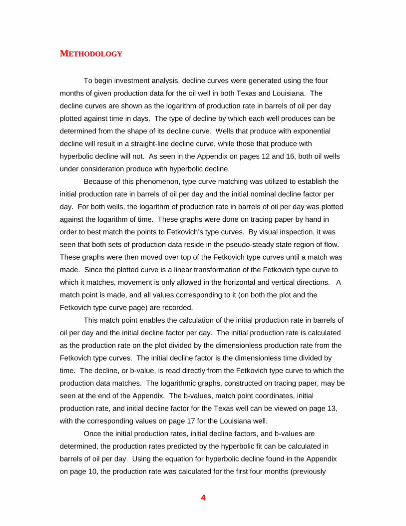
To begin investment analysis, decline curves were generated using the four

months of given production data for the oil well in both Texas and Louisiana. The

decline curves are shown as the logarithm of production rate in barrels of oil per day

plotted against time in days. The type of decline by which each well produces can be

determined from the shape of its decline curve. Wells that produce with exponential

decline will result in a straight-line decline curve, while those that produce with

hyperbolic decline will not. As seen in the Appendix on pages 12 and 16, both oil wells

under consideration produce with hyperbolic decline.

Because of this phenomenon, type curve matching was utilized to establish the

initial production rate in barrels of oil per day and the initial nominal decline factor per

day. For both wells, the logarithm of production rate in barrels of oil per day was plotted

against the logarithm of time. These graphs were done on tracing paper by hand in

order to best match the points to Fetkovich’s type curves. By visual inspection, it was

seen that both sets of production data reside in the pseudo-steady state region of flow.

These graphs were then moved over top of the Fetkovich type curves until a match was

made. Since the plotted curve is a linear transformation of the Fetkovich type curve to

which it matches, movement is only allowed in the horizontal and vertical directions. A

match point is made, and all values corresponding to it (on both the plot and the

Fetkovich type curve page) are recorded.

This match point enables the calculation of the initial production rate in barrels of

oil per day and the initial decline factor per day. The initial production rate is calculated

as the production rate on the plot divided by the dimensionless production rate from the

Fetkovich type curves. The initial decline factor is the dimensionless time divided by

time. The decline, or b-value, is read directly from the Fetkovich type curve to which the

production data matches. The logarithmic graphs, constructed on tracing paper, may be

seen at the end of the Appendix. The b-values, match point coordinates, initial

production rate, and initial decline factor for the Texas well can be viewed on page 13,

with the corresponding values on page 17 for the Louisiana well.

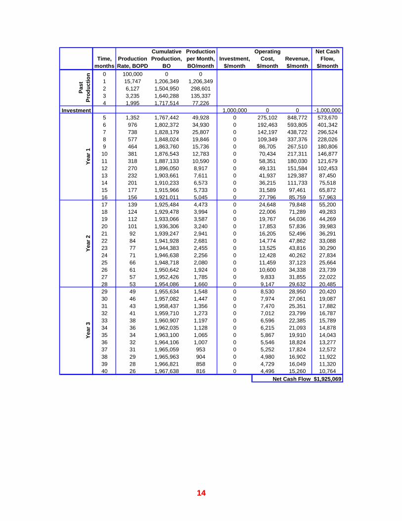
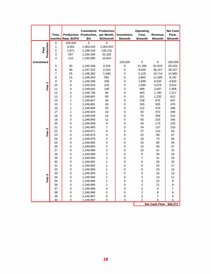
Once the initial production rates, initial decline factors, and b-values are

determined, the production rates predicted by the hyperbolic fit can be calculated in

barrels of oil per day. Using the equation for hyperbolic decline found in the Appendix

on page 10, the production rate was calculated for the first four months (previously

55

produced and, thus, not considered later in the net present value computations) and the

next three years. The cumulative production in barrels of oil was then determined for all

forty months using the equation for hyperbolic decline in the Appendix on page 10.

Then, the change in cumulative production gave way to the oil production per month

predicted by the hyperbolic fit. The values of production rate, cumulative production,

and oil production per month for the first four months (previously produced) and the next

three years may be viewed on page 14 for Texas and page 18 for Louisiana.

After the predicted production for each month was established, net present value

profile was chosen as the yardstick of preference. First, the investment for each well

was determined. The amount of investment for both wells were given ($1,000,000 for

Texas and $100,000 for Louisiana) and were assumed as a lump sum spent before any

production under new ownership occurred. Next, the previously calculated oil production

for each month and the given production cost per barrel of oil produced ($5.51 for Texas

and $4.93 for Louisiana) were used to find the operating costs each month for both

wells. The revenue generated for each month was then calculated using the oil

production for each month and the price of the crude per barrel ($17.00 for Texas and

$18.95 for Louisiana, with an assumed price increase of five percent per year for both

wells).

In order to generate net cash flow values for each month, the investment and

operating costs were subtracted from the revenue. The net present value for each

month was generated using the equation found in the Appendix on page 11. It is

important to note that the interest rate is converted to a monthly interest rate. The

monthly net present values were then summed to find the net present value at each

interest rate for both wells. The monthly net cash flows were also summed to find the

net present value for each well at an interest rate of zero percent. These values can be

seen for Texas on pages 14 and 15 and pages 18 and 19 for Louisiana. Finally, the net

present values for each well were plotted against their corresponding interest rate in

order to obtain a graph of the net present value profile (seen on page 20 of the

Appendix).

66

RREESSUULLTTSS && DDIISSCCUUSSSSIIOONN

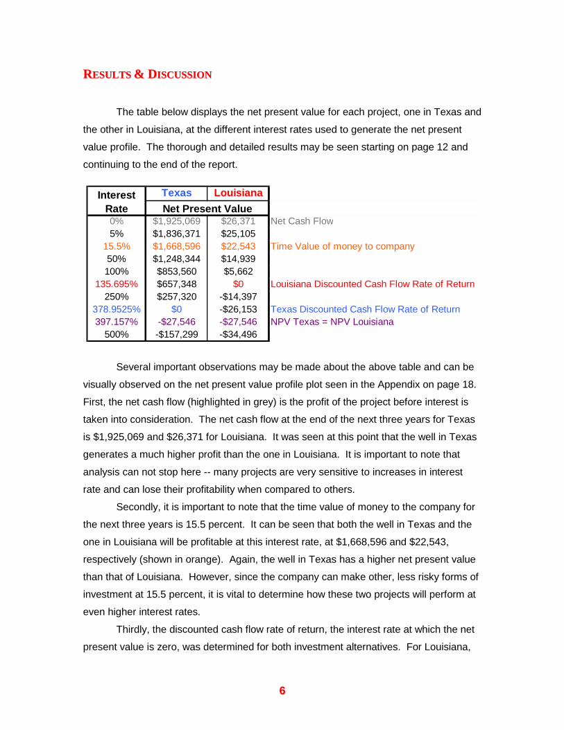
The table below displays the net present value for each project, one in Texas and

the other in Louisiana, at the different interest rates used to generate the net present

value profile. The thorough and detailed results may be seen starting on page 12 and

continuing to the end of the report.

Several important observations may be made about the above table and can be

visually observed on the net present value profile plot seen in the Appendix on page 18.

First, the net cash flow (highlighted in grey) is the profit of the project before interest is

taken into consideration. The net cash flow at the end of the next three years for Texas

is $1,925,069 and $26,371 for Louisiana. It was seen at this point that the well in Texas

generates a much higher profit than the one in Louisiana. It is important to note that

analysis can not stop here -- many projects are very sensitive to increases in interest

rate and can lose their profitability when compared to others.

Secondly, it is important to note that the time value of money to the company for

the next three years is 15.5 percent. It can be seen that both the well in Texas and the

one in Louisiana will be profitable at this interest rate, at $1,668,596 and $22,543,

respectively (shown in orange). Again, the well in Texas has a higher net present value

than that of Louisiana. However, since the company can make other, less risky forms of

investment at 15.5 percent, it is vital to determine how these two projects will perform at

even higher interest rates.

Thirdly, the discounted cash flow rate of return, the interest rate at which the net

present value is zero, was determined for both investment alternatives. For Louisiana,

Texas Louisiana

0% $1,925,069 $26,371 Net Cash Flow5% $1,836,371 $25,105

15.5% $1,668,596 $22,543 Time Value of money to company50% $1,248,344 $14,939100% $853,560 $5,662

135.695% $657,348 $0 Louisiana Discounted Cash Flow Rate of Return250% $257,320 -$14,397

378.9525% $0 -$26,153 Texas Discounted Cash Flow Rate of Return397.157% -$27,546 -$27,546 NPV Texas = NPV Louisiana

500% -$157,299 -$34,496

Net Present ValueInterest

Rate

77

the discounted cash flow rate of return is approximately 136 (denoted in red), while it

was nearly 379 percent for Texas (emphasized in blue). Thus, the Texas well, can

tolerate much higher interest rates than the one in Louisiana. This is true even though it

is actually the Louisiana project that is less sensitive to changes in interest rate. This

means that a change in interest rate will result in a smaller change in net present value

for the well in Louisiana than that of the one in Texas. (Observe the steepness of the

slopes on the net present value profile plot.) This, again, reemphasizes that the Texas

well is a more profitable investment than the oil well in Louisiana. However, since both

of these interest rates are very high, it is safe to say that neither project will lose money if

implemented.

Finally, a vital part of the net present value profile graph is that of the intersection

of the two projects (shown in purple in the above table and on the net present value

profile plot). At this particular interest rate, both projects make the same amount of

money. It is also at this interest rate that the profitability of the projects switches -- the

project that had a lower net present value at lower interest rates will have a higher net

present value than its competitor at higher interest rates. For this analysis, however, this

intersection (at about a 397 percent interest rate) is not very vital since neither project is

profitable (-$27,546).

88

CCOONNCCLLUUSSIIOONN

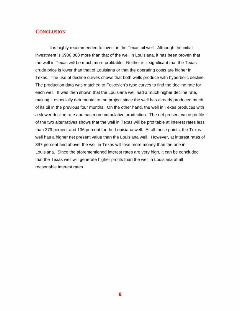
It is highly recommended to invest in the Texas oil well. Although the initial

investment is $900,000 more than that of the well in Louisiana, it has been proven that

the well in Texas will be much more profitable. Neither is it significant that the Texas

crude price is lower than that of Louisiana or that the operating costs are higher in

Texas. The use of decline curves shows that both wells produce with hyperbolic decline.

The production data was matched to Fetkovich's type curves to find the decline rate for

each well. It was then shown that the Louisiana well had a much higher decline rate,

making it especially detrimental to the project since the well has already produced much

of its oil in the previous four months. On the other hand, the well in Texas produces with

a slower decline rate and has more cumulative production. The net present value profile

of the two alternatives shows that the well in Texas will be profitable at interest rates less

than 379 percent and 136 percent for the Louisiana well. At all these points, the Texas

well has a higher net present value than the Louisiana well. However, at interest rates of

397 percent and above, the well in Texas will lose more money than the one in

Louisiana. Since the aforementioned interest rates are very high, it can be concluded

that the Texas well will generate higher profits than the well in Louisiana at all

reasonable interest rates.

99

RREEFFEERREENNCCEESS

Mohaghegh, Shahab D. Ph.D. Class notes and handouts. Petroleum and Natural Gas

Engineering 241: Oil Property Evaluation. West Virginia University: Morgantown,

West Virginia. 1999.

Thompson, Robert S. and John D. Wright. "Oil Property Evaluation." 2nd ed.

Thompson-Wright Associates: Golden, Colorado. 1985.

1100

AAPPPPEENNDDIIXX

Calculations

1.) Hyperbolic Decline

Producing Rate:

q = qi(1 + bDit)- 1 / b

Cumulative Production:

Np = [ ]bbi

i

b

qqbD

qi −− −−

11

)1(

where: q = producing rate at time t, STB/dayqi = producing rate at time 0, STB/dayDi = initial nominal decline rate (t = 0), 1 / dayb = hyperbolic exponentt = time, daysNp = Cumulative Production, STB

2.) Type Curve Analysis (Pseudo-Steady State Region)

Initial Flow Rate:

qi = TDqq

Initial Decline Rate:

Di = t

tDT

where: qi = producing rate at time 0, STB/dayq = producing rate at time t, STB/dayqTD = dimensionless producing rateDi = initial nominal decline rate (t = 0), 1 / daytDT = dimensionless time

1111

3.) Economic Analysis

Net Present Value:

NPV = ∑= +

L

jj

j

iNCF

0 )1(

where: NPV = net present value, $NCFj = net cash flow for period j, $i = interest rate (monthly)j = period (month)

1122

Texas Well Decline Curve

1,000

10,000

100,000

0 20 40 60 80 100 120 140

Time, days

Rat

e, B

OPD

1133

TEXASPrice, $/BO Op Cost, $/BO

17.00 5.51

Time, daysProduction Rate, BOPD

1 92,8002 81,3904 69,9806 58,8008 50,10010 41,80020 25,00030 15,00040 10,50050 8,00070 4,800

100 2,600120 2,000

b = 0.5q = 10,000 BOPD

qDd = 0.1t = 1 days

tDd = 0.1

qi = q/qDd = 100,000 BOPDDi = tDd/t = 0.1 per day

Match Point

Price increase by 5%

1144

Time, months

Production Rate, BOPD

Cumulative Production,

BO

Production per Month, BO/month

Investment, $/month

Operating Cost,

$/monthRevenue, $/month

Net Cash Flow,

$/month0 100,000 0 01 15,747 1,206,349 1,206,3492 6,127 1,504,950 298,6013 3,235 1,640,288 135,3374 1,995 1,717,514 77,226

Investment 1,000,000 0 0 -1,000,0005 1,352 1,767,442 49,928 0 275,102 848,772 573,6706 976 1,802,372 34,930 0 192,463 593,805 401,3427 738 1,828,179 25,807 0 142,197 438,722 296,5248 577 1,848,024 19,846 0 109,349 337,376 228,0269 464 1,863,760 15,736 0 86,705 267,510 180,80610 381 1,876,543 12,783 0 70,434 217,311 146,87711 318 1,887,133 10,590 0 58,351 180,030 121,67912 270 1,896,050 8,917 0 49,131 151,584 102,45313 232 1,903,661 7,611 0 41,937 129,387 87,45014 201 1,910,233 6,573 0 36,215 111,733 75,51815 177 1,915,966 5,733 0 31,589 97,461 65,87216 156 1,921,011 5,045 0 27,796 85,759 57,96317 139 1,925,484 4,473 0 24,648 79,848 55,20018 124 1,929,478 3,994 0 22,006 71,289 49,28319 112 1,933,066 3,587 0 19,767 64,036 44,26920 101 1,936,306 3,240 0 17,853 57,836 39,98321 92 1,939,247 2,941 0 16,205 52,496 36,29122 84 1,941,928 2,681 0 14,774 47,862 33,08823 77 1,944,383 2,455 0 13,525 43,816 30,29024 71 1,946,638 2,256 0 12,428 40,262 27,83425 66 1,948,718 2,080 0 11,459 37,123 25,66426 61 1,950,642 1,924 0 10,600 34,338 23,73927 57 1,952,426 1,785 0 9,833 31,855 22,02228 53 1,954,086 1,660 0 9,147 29,632 20,48529 49 1,955,634 1,548 0 8,530 28,950 20,42030 46 1,957,082 1,447 0 7,974 27,061 19,08731 43 1,958,437 1,356 0 7,470 25,351 17,88232 41 1,959,710 1,273 0 7,012 23,799 16,78733 38 1,960,907 1,197 0 6,596 22,385 15,78934 36 1,962,035 1,128 0 6,215 21,093 14,87835 34 1,963,100 1,065 0 5,867 19,910 14,04336 32 1,964,106 1,007 0 5,546 18,824 13,27737 31 1,965,059 953 0 5,252 17,824 12,57238 29 1,965,963 904 0 4,980 16,902 11,92239 28 1,966,821 858 0 4,729 16,049 11,32040 26 1,967,638 816 0 4,496 15,260 10,764

$1,925,069Net Cash Flow

Past

Pr

oduc

tion

Year

1Ye

ar 2

Year

3

1155

Time, months

Net Cash Flow,

$/monthNPV 5%, $/month

NPV 15.5%,

$/monthNPV 50%, $/month

NPV 100%, $/month

NPV 135.695%, $/month

NPV 250%, $/month

NPV 378.9525%,

$/month

NPV 397.157%, $/month

NPV 500%, $/month

01234

Investment -1,000,000 -1,000,000 -1,000,000 -1,000,000 -1,000,000 -1,000,000 -1,000,000 -1,000,000 -1,000,000 -1,000,0005 573,670 571,289 566,354 550,723 529,541 515,390 474,761 435,988 431,018 404,9436 401,342 398,018 391,172 369,877 341,972 323,938 274,879 231,814 226,559 199,9777 296,524 292,848 285,324 262,346 233,224 215,022 168,074 130,166 125,765 104,2938 228,026 224,265 216,616 193,673 165,553 148,553 106,964 76,074 72,664 56,6139 180,806 177,085 169,568 147,424 121,172 105,823 70,190 45,843 43,289 31,686

10 146,877 143,258 135,991 114,969 90,862 77,232 47,188 28,303 26,421 18,17011 121,679 118,188 111,224 91,435 69,483 57,482 32,352 17,820 16,446 10,62512 102,453 99,101 92,456 73,909 54,004 43,483 22,544 11,403 10,404 6,31513 87,450 84,238 77,911 60,562 42,550 33,345 15,925 7,397 6,672 3,80514 75,518 72,442 66,422 50,207 33,918 25,870 11,381 4,855 4,329 2,31915 65,872 62,927 57,199 42,042 27,310 20,273 8,216 3,218 2,837 1,42816 57,963 55,142 49,690 35,515 22,182 16,027 5,983 2,152 1,876 88717 55,200 52,296 46,718 32,469 19,500 13,712 4,715 1,558 1,342 59618 49,283 46,496 41,178 27,829 16,071 10,999 3,484 1,057 900 37619 44,269 41,592 36,517 23,998 13,325 8,876 2,590 722 608 23820 39,983 37,410 32,561 20,807 11,109 7,202 1,936 495 412 15221 36,291 33,814 29,177 18,131 9,308 5,873 1,454 342 281 9722 33,088 30,702 26,263 15,869 7,833 4,811 1,097 237 193 6323 30,290 27,990 23,736 13,946 6,620 3,956 831 165 132 4024 27,834 25,613 21,533 12,303 5,615 3,266 632 115 91 2625 25,664 23,518 19,601 10,890 4,779 2,706 482 81 63 1726 23,739 21,663 17,899 9,670 4,080 2,248 369 57 44 1127 22,022 20,014 16,393 8,612 3,494 1,874 284 40 31 728 20,485 18,540 15,055 7,690 3,000 1,566 218 28 21 529 20,420 18,404 14,815 7,359 2,761 1,402 180 21 16 330 19,087 17,132 13,672 6,604 2,382 1,178 139 15 11 231 17,882 15,983 12,645 5,939 2,060 991 108 11 8 132 16,787 14,942 11,719 5,352 1,785 836 84 8 6 133 15,789 13,995 10,882 4,833 1,550 706 65 6 4 134 14,878 13,133 10,123 4,372 1,348 598 51 4 3 035 14,043 12,345 9,434 3,962 1,174 507 40 3 2 036 13,277 11,623 8,805 3,596 1,025 431 31 2 1 037 12,572 10,960 8,231 3,269 896 366 24 1 1 038 11,922 10,350 7,706 2,975 784 312 19 1 1 039 11,320 9,787 7,224 2,712 687 266 15 1 1 040 10,764 9,267 6,781 2,476 603 228 12 1 0 0

$1,925,069 $1,836,371 $1,668,596 $1,248,344 $853,560 $657,348 $257,320 $0 -$27,546 -$157,2990% 5% 15.5% 50% 100% 135.695% 250% 378.9525% 397.157% 500%Interest Rate

Past

Pr

oduc

tion

Year

1Ye

ar 2

Year

3

Total NPV

1166

Louisiana Well Decline Curve

100

1,000

10,000

100,000

0 20 40 60 80 100 120 140

Time, days

Rat

e, B

OPD

1177

LOUISIANAPrice, $/BO Op Cost, $/BO

18.95 4.93

Time, daysProduction Rate, BOPD

1 93,0002 81,5004 70,0006 53,0008 43,00010 38,50020 18,00030 9,00040 5,00050 2,90070 1,100

100 370120 200

b = 0.2q = 10,000 BOPD

qDd = 0.1t = 10 days

tDd = 1

qi = q/qDd = 100,000 BOPDDi = tDd/t = 0.1 per day

Price increase by 5%

Match Point

1188

Time, months

Production Rate, BOPD

Cumulative Production,

BO

Production per Month, BO/month

Investment, $/month

Operating Cost,

$/monthRevenue, $/month

Net Cash Flow,

$/month0 100,000 0 01 9,302 1,063,033 1,063,0332 1,871 1,198,164 135,1313 557 1,230,346 32,1824 210 1,240,990 10,644

Investment 100,000 0 0 -100,0005 93 1,245,308 4,318 0 21,286 81,819 60,5336 46 1,247,322 2,014 0 9,929 38,167 28,2377 25 1,248,362 1,040 0 5,129 19,714 14,5858 14 1,248,943 581 0 2,863 11,005 8,1429 9 1,249,288 345 0 1,699 6,532 4,83310 6 1,249,503 215 0 1,060 4,074 3,01411 4 1,249,642 140 0 689 2,647 1,95812 3 1,249,736 94 0 463 1,780 1,31713 2 1,249,801 65 0 321 1,232 91214 1 1,249,847 46 0 228 875 64715 1 1,249,881 34 0 165 635 47016 1 1,249,906 25 0 122 470 34817 1 1,249,924 19 0 92 372 28018 0 1,249,939 14 0 70 284 21419 0 1,249,950 11 0 55 220 16620 0 1,249,958 9 0 43 173 13021 0 1,249,965 7 0 34 137 10322 0 1,249,971 6 0 27 110 8323 0 1,249,975 4 0 22 89 6724 0 1,249,979 4 0 18 73 5525 0 1,249,982 3 0 15 60 4526 0 1,249,984 2 0 12 49 3727 0 1,249,986 2 0 10 41 3128 0 1,249,988 2 0 9 35 2629 0 1,249,990 1 0 7 31 2330 0 1,249,991 1 0 6 26 2031 0 1,249,992 1 0 5 22 1732 0 1,249,993 1 0 5 19 1533 0 1,249,994 1 0 4 16 1334 0 1,249,994 1 0 3 14 1135 0 1,249,995 1 0 3 12 936 0 1,249,995 1 0 3 11 837 0 1,249,996 0 0 2 9 738 0 1,249,996 0 0 2 8 639 0 1,249,997 0 0 2 7 640 0 1,249,997 0 0 2 6 5

$26,371Net Cash Flow

Past

Pr

oduc

tion

Year

1Ye

ar 2

Year

3

1199

Time, months

Net Cash Flow,

$/monthNPV 5%, $/month

NPV 15.5%, $/month

NPV 50%, $/month

NPV 100%,

$/month

NPV 135.695%, $/month

NPV 250%,

$/month

NPV 378.9525%,

$/month

NPV 397.157%, $/month

NPV 500%,

$/month01234

Investment -100,000 -100,000 -100,000 -100,000 -100,000 -100,000 -100,000 -100,000 -100,000 -100,0005 60,533 60,282 59,761 58,112 55,877 54,384 50,096 46,005 45,481 42,7296 28,237 28,003 27,522 26,023 24,060 22,791 19,340 16,310 15,940 14,0707 14,585 14,404 14,034 12,904 11,472 10,576 8,267 6,402 6,186 5,1308 8,142 8,008 7,735 6,916 5,911 5,304 3,819 2,716 2,595 2,0229 4,833 4,733 4,532 3,940 3,239 2,828 1,876 1,225 1,157 847

10 3,014 2,940 2,791 2,359 1,864 1,585 968 581 542 37311 1,958 1,902 1,790 1,471 1,118 925 521 287 265 17112 1,317 1,274 1,188 950 694 559 290 147 134 8113 912 878 812 631 444 348 166 77 70 4014 647 621 569 430 291 222 98 42 37 2015 470 449 408 300 195 145 59 23 20 1016 348 331 298 213 133 96 36 13 11 517 280 265 237 164 99 69 24 8 7 318 214 202 179 121 70 48 15 5 4 219 166 156 137 90 50 33 10 3 2 120 130 122 106 68 36 23 6 2 1 021 103 96 83 52 26 17 4 1 1 022 83 77 66 40 20 12 3 1 0 023 67 62 52 31 15 9 2 0 0 024 55 50 42 24 11 6 1 0 0 025 45 41 34 19 8 5 1 0 0 026 37 34 28 15 6 4 1 0 0 027 31 28 23 12 5 3 0 0 0 028 26 24 19 10 4 2 0 0 0 029 23 21 17 8 3 2 0 0 0 030 20 18 14 7 2 1 0 0 0 031 17 15 12 6 2 1 0 0 0 032 15 13 10 5 2 1 0 0 0 033 13 11 9 4 1 1 0 0 0 034 11 10 7 3 1 0 0 0 0 035 9 8 6 3 1 0 0 0 0 036 8 7 5 2 1 0 0 0 0 037 7 6 5 2 1 0 0 0 0 038 6 6 4 2 0 0 0 0 0 039 6 5 4 1 0 0 0 0 0 040 5 4 3 1 0 0 0 0 0 0

$26,371 $25,105 $22,543 $14,939 $5,662 $0 -$14,397 -$26,153 -$27,546 -$34,4960% 5% 15.5% 50% 100% 135.695% 250% 378.9525% 397.157% 500%

Total NPVInterest Rate

Past

Pr

oduc

tion

Year

1Ye

ar 2

Year

3

2200

Net Present Value Profile

-$250,000

$0

$250,000

$500,000

$750,000

$1,000,000

$1,250,000

$1,500,000

$1,750,000

$2,000,000

0% 50% 100% 150% 200% 250% 300% 350% 400% 450% 500%

Interest Rate

Net

Pre

sent

Val

ue, $

Texas Well Net Present Value Louisiana Well Net Present Value

15.5

%$1,668,596

$22,543NPV Texas = NPV Louisiana

397.157%, -$27,546$0 $0

135.

695%

378

.952

5%