CYLINDER BUCKLING: THE MOUNTAIN PASS AS AN ORGANIZINGCENTER

JIRI HORAK∗, GABRIEL J. LORD† , AND MARK A. PELETIER‡

Abstract. We revisit the classical problem of the buckling of a long thin axially compressed cylindrical shell.By examining the energy landscape of the perfect cylinder we deduce an estimate of the sensitivity of the shell toimperfections. Key to obtaining this is the existence of a mountain pass point for the system. We prove the existenceon bounded domains of such solutions for all most all loads and then numerically compute example mountain passsolutions. Numerically the mountain pass solution with lowest energy has the form of a single dimple. We interpretthese results and validate the lower bound against some experimental results available in the literature.

Key words. Imperfection sensitivity, subcritical bifurcation, single dimple

1. Introduction.

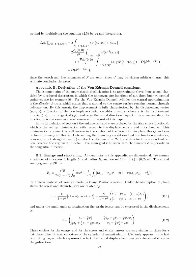
1.1. Buckling of cylinders under axial loading. A classical problem in structural en-gineering is the prediction of the load-carrying capacity of an axially-loaded cylinder. As wellas being a commonly used structural element, the axially-loaded cylinder is also the archetypeof unstable, imperfection-sensitive buckling, and this has led to a large body of theoretical andexperimental research.

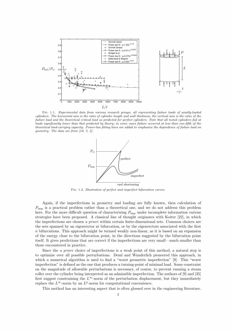
In the decades before and after the second world war a central problem was to understandthe large discrepancy between theoretical predictions and experimental observations, as shown inFigure 1.1. A variety of different explanations has been put forward, but with the experimentalwork of Tennyson [30] and the theoretical work of Almroth [1] it became clear that this discrepancyis mostly due to imperfections in loading conditions and in the shape of the specimens. Furtherexperimental and theoretical work by many others has confirmed this conclusion [14, 33, 36].

For near-perfect cylinders the linear and weakly non-linear theories (see Section 1.2) ade-quately describe the experimental buckling load1 and the deformation just before failure (seee.g. [4]). Cylinders used in practical applications, however, are far too imperfect for this weaklynon-linear theory to apply, and from a practical point of view the problem of predicting the failureload is still open.

In fact there is good reason to believe that it will never be possible to accurately predictfailure loads for cylinders that are used in practice. For simple materials, such as metals, it isbelieved that current numerical methods can describe the local material behaviour with enoughaccuracy that correct prediction of the complete behaviour of the cylinder—including its failure—is feasible. This could be achieved provided the geometrical and material imperfections as well asthe loading conditions are determined in sufficient detail. The difficulty lies in the qualifier “insufficient detail”, since an extremely accurate measurement of geometric imperfections would benecessary [4], and in the design phase both the loading conditions and the geometrical and materialimperfections in the finalized product are only known in vague terms. Therefore, in recent decadesthe attention of theoretical research has turned to characterizing the failure load in weaker ways,preferably in the form of a lower (safe) bound.

1.2. Characterizing sensitivity to imperfections. Viewed as a bifurcation problem, thebuckling of the cylinder is a subcritical symmetry-breaking pitchfork bifurcation (Figure 1.2).Generically, imperfections in the structure eliminate the bifurcation and round off the branch ofsolutions2, resulting in a turning-point at a load Pimp strictly below the critical (bifurcation) loadPcr of the perfect structure. In an experiment in which the load is slowly increased, the systemwill fail (i.e. make a large jump in state space) at load Pimp.

∗Universitat Koln, Germany†Heriot-Watt University, Edinburgh, United Kingdom‡Technische Universiteit Eindhoven, The Netherlands1In this paper the terms “experimental buckling load” and “failure load” are used interchangeably2Koiter actually used this elimination of a bifurcation point as a definition of “perfect system” and “perturbed

system” [22]

1

0 1000 2000 3000 4000 5000 6000 7000 8000 9000 100000

0.1

0.2

0.3

0.4

0.5

0.6

0.7

0.8

0.9

1

Donnell (steel)Power law fit : y=1.03x−0.176

Donnell (brass)Power law fit : y=0.511x−0.0879

Bridget et alPower law fit : y=0.373x−0.00504

Ballerstedt & WagnerPower law fit : y=4.22x−0.374

Pfail/Pcr

L/t

P

L

t

Fig. 1.1. Experimental data from various research groups, all representing failure loads of axially-loadedcylinders. The horizontal axis is the ratio of cylinder length and wall thickness; the vertical axis is the ratio of thefailure load and the theoretical critical load as predicted for perfect cylinders. Note that all tested cylinders fail atloads significantly lower than that predicted by theory; in some cases failure occurred at less than one-fifth of thetheoretical load-carrying capacity. Power-law fitting lines are added to emphasize the dependence of failure load ongeometry. The data are from [10, 7, 5].

Pcr

Pimp

perfect

imperfect

end shortening

Fig. 1.2. Illustration of perfect and imperfect bifurcation curves.

Again, if the imperfections in geometry and loading are fully known, then calculation ofPimp is a practical problem rather than a theoretical one, and we do not address this problemhere. For the more difficult question of characterizing Pimp under incomplete information variousstrategies have been proposed. A classical line of thought originates with Koiter [22], in whichthe imperfections are chosen a priori within certain finite-dimensional sets. Common choices arethe sets spanned by an eigenvector at bifurcation, or by the eigenvectors associated with the firstn bifurcations. This approach might be termed weakly non-linear, as it is based on an expansionof the energy close to the bifurcation point, in the directions suggested by the bifurcation pointitself. It gives predictions that are correct if the imperfections are very small—much smaller thanthose encountered in practice.

Since the a priori choice of imperfections is a weak point of this method, a natural step isto optimize over all possible perturbations. Deml and Wunderlich pioneered this approach, inwhich a numerical algorithm is used to find a “worst geometric imperfection” [9]. This “worstimperfection” is defined as the one that produces a turning-point of minimal load. Some constrainton the magnitude of allowable perturbations is necessary, of course, to prevent running a steamroller over the cylinder being interpreted as an admissible imperfection. The authors of [9] and [35]first suggest constraining the L∞-norm of the perturbation displacement, but they immediatelyreplace the L∞-norm by an Lp-norm for computational convenience.

This method has an interesting aspect that is often glossed over in the engineering literature.2

By definition the failure load obtained by this method is a lower bound for the failure load of allsystems that have perturbations of less or equal magnitude. The measure of magnitude is definedby the choice of constraint. Therefore the choice of constraint on the imperfections is a criticalone, since it implicitly defines a class of imperfections that produce the same or higher failureload.

1.3. Main results. In this paper we follow a related, but distinct, line of reasoning. Insteadof studying actual behaviour of imperfect cylinders, we deduce an estimate of the sensitivity toimperfections from the energy landscape of the perfect cylinder. The final result is a lower boundon the failure load similar to above, and the approach gives additional insight into the problem.

The key result is the existence of a mountain-pass point, an equilibrium state that sits astraddlein the energy landscape between two valleys; one valley surrounds the unbuckled state, and theother contains many buckled, large-deformation states.

This mountain-pass point has a number of interesting properties:1. It has the appearance of a single-dimple solution, a small buckle in the form of a single

dent (see Figure 1.3 (a)). Single-dimple deformations have appeared in the engineeringliterature in a number of different ways (see Section 6), but theoretical understanding ofthis phenomenon is still lacking. Localization (concentration) of deformation is knowncommonly to appear in extended structures [21], and in the cylinder localization in theaxial direction has been studied theoretically and numerically [20, 24, 25]. Whether local-ization is possible in the tangential direction has been an open problem for some time; it isinteresting that our simulations for the perfect structure show solutions that are localizedin both axial and tangential directions.

2. Like all mountain-pass points this single-dimple solution is unstable, in the sense that thereare directions in state space in which the energy decreases. In one direction the dimpleroughly shrinks and disappears, and in the opposite direction it grows and multiplies(Figure 1.3 (b-c)). It is remarkable, however, that our numerical results indicate that thesingle-dimple solution has an alternative characterization as a constrained global minimizer(a global minimizer of the strain energy under prescribed end shortening).

3. The equations can be rescaled so that the only remaining parameters are the load leveland the domain. The geometry of the mountain-pass solution we calculate even appearsto be independent of the domain size.

This mountain-pass point is central in an estimate of the sensitivity to perturbations. Forthe system to escape from the neighbourhood of the unbuckled state, it must possess at least theenergy associated with this mountain-pass point. The mountain-pass energy level is therefore anindication of the degree of stability of the unbuckled state. Implicitly it defines a class of perturba-tions for which the unbuckled state is stable. This approach is related to the “perturbation-energy”approach first suggested by Kroplin and co-workers [23, 11, 32], but differs in some essential points;see the discussion in Section 5.

1.4. Methods. We use both analytical and numerical methods. In Section 2 we introducethe Von Karman-Donnell equations, which form the basis of this paper, and rescale them in anappropriate manner. In Section 3 we present the functional setting that we use, show that theenergy functional has the geometry associated with a mountain pass, and prove the existenceof mountain-pass points (Lemma 3.5). There are certain interesting technical issues. By theirlocalized nature, single-dimple solutions are most naturally defined on an unbounded domain;however, we are only able to prove existence of mountain-pass points on bounded domains, andconsequently we work on finite domains that become large in the limit of thin shells. Similarly,the non-coercive nature of the energy functional implies that we prove existence of mountain-passpoints for almost all load levels (see Lemma 3.4).

In Section 4 we turn to numerical investigation. We use a variety of different algorithmsto find solutions of the discretized Von Karman-Donnell equations. With a discrete mountainpass algorithm we find solutions that are, by construction, mountain-pass points. The solutionof Figure 1.3 (a) was found in this manner. With a constrained gradient flow we also find localminima of the strain energy under prescribed end shortening. Some of these solutions appear

3

(a)

wMP

(b) (c)

−10 −5 0 5 10

−15

−10

0

5

V (λ)

(a)

(b)JJJ

(c)

Fλ(w

)

distance in X

(a) . . . V (λ) = Fλ(wMP) ≈ 4.84(b) . . . Fλ(w) ≈ −15.57(c) . . . Fλ(w) ≈ −5.5 · 104

Fig. 1.3. Part (a) shows a numerical computation of a solution wMP that is a mountain-pass point of theenergy Fλ for a load λ = 1.5. We show both the graph of wMP(x, y) as well as its rendering on a cylinder. AtwMP there exist two directions in the state space X in which the energy Fλ decreases. By perturbing wMP in thesedirections and following a gradient flow of Fλ we move away from wMP. In one direction the dimple shrinks tozero (not shown) and in the opposite it grows in amplitude and extent (figures (b) and (c)).

to coincide with those found by the discrete mountain pass algorithm, and the mountain passsolutions are stable under this gradient flow. These observations lead us to conjecture that theglobal mountain pass solution is also a global constrained minimizer of the strain energy. By aconstrained version of the discrete mountain pass algorithm we also find critical points of higherMorse index.

Section 5 is devoted to an interpretation of these results in the context of imperfection sensi-tivity, as mentioned above, and in Section 6 we wrap up with the main conclusions.

2. The Von Karman-Donnell equations. We consider a cylindrical shell of radius R,thickness t, Young’s modulus E, and Poisson’s ratio ν, that is subject to a compressive axialforce P . In dimensionless form the Von Karman-Donnell equations are given by

ε2∆2w + λwxx − φxx − 2[w, φ] = 0, (2.1)

∆2φ+ [w,w] + wxx = 0, (2.2)

where subscripts x and y denote differentiation with respect to the spatial variables, and thebracket [·, ·] is defined as

[a, b] =12axxbyy +

12ayybxx − axybxy.

The function w is the inward radial displacement measured from a unbuckled (fundamental) state,φ is the Airy stress function, ε2 = t2(192π4R2(1− ν2))−1 and the nondimensional load parameter

4

is given by λ = P (8π3ERt)−1. The unknowns w and φ are defined on the two-dimensional spatialdomain (−`, `)× (−1/2, 1/2), where x ∈ (−`, `) is the axial and y ∈ (−1/2, 1/2) is the tangentialcoordinate. Since the y-domain (−1/2, 1/2) represents the circumference of the cylinder, thefunctions w and φ are periodic in y; at the axial ends x ∈ −`, ` they satisfy the boundaryconditions

wx = (∆w)x = φx = (∆φ)x = 0.

In Appendix B we discuss the derivation of this formulation.

Equations (2.1-2.2) can be rescaled to be parameter-independent in all but the domain ofdefinition and load parameter, by substituting

w 7→ εw, φ 7→ ε2φ, x 7→ ε1/2x, y 7→ ε1/2y, λ 7→ ελ. (2.3)

so that the equations become

∆2w + λwxx − φxx − 2 [w, φ] = 0, (2.4)

∆2φ+ [w,w] + wxx = 0. (2.5)

The domain of definition of w and φ is now

Ω := (−`ε−1/2, `ε−1/2)× (− 12ε−1/2, 1

2ε−1/2),

which expands to R2 as ε→ 0. When not indicated otherwise we choose the aspect ratio 2` = 1;in Section 4.3 we comment on the influence of domain size and aspect ratio.

The boundary conditions for w and φ now are

w is periodic in y, and wx = (∆w)x = 0 at x = ± 12ε−1/2, (2.6a)

φ is periodic in y, and φx = (∆φ)x = 0 at x = ± 12ε−1/2. (2.6b)

Equations (2.4–2.5) are related to the stored energy E and the average axial shortening Sgiven by

E(w) :=12

∫Ω

(∆w2 + ∆φ2

), and S(w) :=

12

∫Ω

w2x. (2.7)

Note that the function φ in (2.7) is determined from w by solving (2.5) with boundary condi-tions (2.6b). Furthermore, solutions of (2.4–2.5) are stationary points of the total potential

Fλ(w) := E(w)− λS(w) (2.8)

and are also stationary points of E under the constraint of constant S. We use both propertiesbelow.

3. The mountain pass: overview. We briefly recall the general context of the Mountain-Pass Theorem of Ambrosetti and Rabinowitz [2]. Let I be a functional defined on a Banach spaceX, and let w1, w2 be two distinct points in X. Consider the family Γ of all paths in X connectingw1 and w2 and define

c = infγ∈Γ

maxw∈γ

I(w) , (3.1)

that is the infimum of the maxima of the functional I along paths in Γ. If c > maxI(w1), I(w2),then the paths have to cross a “mountain range” and one may conjecture that there exists a criticalpoint wMP of I at the level c, called a mountain pass point.

We will apply this idea to the Von Karman-Donnell-equations in the following way. We takefor I the total potential Fλ (see (2.8)) at some fixed value of λ, and for the end point w1 theorigin. We will obtain a mountain-pass solution by the following steps:

5

MP1. We first show that w1 = 0 is a local minimizer: there are %, α > 0 such that Fλ(w) ≥ αfor all w with ‖w‖X = % (Lemma 3.1);

MP2. If ε is small enough, then there exists w2 with Fλ(w2) ≤ 0 (Corollary 3.3).MP3. Given a sequence of paths γn that approximates the infimum in (3.1), we extract a (Palais-

Smale) sequence of points wn ∈ γn, each one close to the maximum along γn, and showthat this sequence converges in an appropriate manner (Lemmas 3.4 and 3.5).

In this way it follows that there exists a mountain-pass critical point w with Fλ(w) = c,provided that ε is sufficiently small (or that the domain is sufficiently large). For technical reasons(lack of coerciveness of the functional Fλ) this procedure can be performed only for almost all0 < λ < 2 (see Lemma 3.4).

In the rest of this section we detail the steps outlined above.

3.1. Choice of spatial domain. We are interested in mountain-pass solutions of the systemof equations (2.4–2.5) that are quasi-independent of the domain size ε−1/2, in the sense that theyconverge to a non-trivial solution on R2 as ε → 0. This point of view suggests considering theproblem on the whole of R2 rather than on a sequence of domains of increasing size; however,there are two reasons not to do this. To start with, the numerical calculations described below arenecessarily done on a bounded domain; more importantly, for the proof of existence of mountain-pass points boundedness of the domain is necessary. For these reasons we concentrate on boundeddomains, while keeping the context of the unbounded domain in mind.

3.2. Functional setting and linearization. We introduce a functional setting for thefunctions w that is suggested by the linearization of the stored energy functional E. Writingφ = φ1 + φ2, where

∆2φ1 = −wxx and ∆2φ2 = −[w,w], (3.2)

we can expand the energy functional E as

E(w) =12

∫Ω

∆w2 +12

∫Ω

∆φ21 +

∫Ω

∆φ1∆φ2 +12

∫Ω

∆φ22. (3.3)

Since φ2 is quadratic in w, the second derivative of E is given by

d2E(0) · u · v =∫

Ω

∆u∆v +∫

Ω

∆φu1∆φv

1,

where φu,v1 are obtained from u and v by (3.2). Inspired by this linearization of E we define

X =ψ ∈ H2(Ω) : ψx(± 1

2ε−1/2, ·) = 0, ψ is periodic in y, and

∫Ω

ψ = 0

with norm

‖w‖2X =∫

Ω

(∆w2 + ∆φ2

1

),

where φ1 ∈ H2(Ω) is the unique solution of

∆2φ1 = −wxx, φ1 satisfies (2.6b), and∫

Ω

φ1 = 0.

This norm is equivalent to the H2-norm on the set X, and with the appropriate inner product thespace X is a Hilbert space.

We now address the requirements of the mountain pass theorem mentioned above in MP1–MP3.

6

3.3. The origin is a local minimizer. The norm in X is related in a natural manner withthe shortening S, as is demonstrated by the (sharp) estimate

2S(w) =∫

Ω

w2x = −

∫Ω

wwxx =∫

Ω

w∆2φ1 =∫

Ω

∆w∆φ1 ≤12

∫Ω

∆w2 +12

∫Ω

∆φ21 =

12‖w‖2X .

(3.4)This inequality strongly suggests that for λ < 2 the origin is a strict local minimum for thefunctional Fλ(w) = E(w)− λS(w).

Lemma 3.1.1. There exists a constant C, dependent on Ω, such that∣∣∣∣∫

Ω

∆φ1∆φ2

∣∣∣∣ ≤ C ‖w‖3X . (3.5)

2. For any 0 < λ < 2 there exists % > 0 such that

infFλ(w) : ‖w‖X = %

> 0.

Proof. Split φ = φ1 +φ2 as in (3.2), and note that the function ∇φ1 is bounded in L∞ by theSobolev imbedding ψ ∈ H3 :

∫ψ = 0 → L∞:

‖∇φ1‖2L∞ ≤ C∥∥∆2φ1

∥∥2

L2 = C ‖wxx‖2L2 .

The third term on the right-hand side of (3.3) can now be rewritten as∫Ω

∆φ1∆φ2 =∫

Ω

φ1[w,w] =∫

Ω

φ1(wxxwyy − w2xy) =

∫Ω

(φ1ywxwxy − φ1xwxwyy),

which we estimate by∣∣∣∣∫Ω

∆φ1∆φ2

∣∣∣∣ ≤ 2 ‖∇φ1‖L∞ ‖wx‖L2 ‖∆w‖L2 ≤ C ‖wx‖L2 ‖∆w‖2L2 ≤ C√S(w) ‖w‖2X ,

thus proving the first part of the Lemma.Since λ < 2, choose 0 < % < (2−λ)/2C and define η = 1

2 (1−C%−λ/2) > 0. Then on the setC = w : ‖w‖X = %, using (3.4), we find that

Fλ(w) = E(w)− λS(w)

≥ 12‖w‖2X − C

√S(w) ‖w‖2X − λS(w)

≥ %2

2− C%3 1

2− λ

%2

4

=%2

2

(1− C%− λ

2

)= η%2.

Part 2 of this lemma implies that by choosing w1 to be the origin we have shown conditionMP1.

Remark 3.1. Although the inequality (3.4) suggests that the origin should be a local minimizerfor any domain Ω, bounded or not, the proof above only applies to bounded domains. F. Ottohas constructed a proof of this result that is valid on any domain (personal communication).Interestingly, this proof uses not only the cubic energy term

∫Ω

∆φ1∆φ2 but also the quartic term∫Ω

∆φ22, and appears to break down without this latter term.

7

3.4. Periodic solutions exist with negative Fλ. To satisfy MP2 we show in this sectionthat for any λ > 0 functions w ∈ X exist for which Fλ(w) = E(w) − λS(w) < 0. To do this weconstruct a sequence of functions wδ with specific scaling properties:

Lemma 3.2. There exists a sequence of functions wδ, 1-periodic on R2, such that∫[−1/2,1/2]2

w2δx ∼ 1,

∫[−1/2,1/2]2

∆w2δ = O(δ−1),

and∫

[−1/2,1/2]2

∆φ2δ = O(δ2−α) as δ → 0,

for any α > 0. Here the functions wδ and φδ solve equation (2.5) with periodic boundary conditions.In addition, wδ and φδ satisfy the boundary conditions (2.6) on the boundary of [−1/2, 1/2]2.

The proof, given in the Appendix, is inspired by the so-called Yoshimura pattern [37], afolding pattern by which a flat sheet of paper, or a cylindrical sheet of thin material, can be foldedinto a macroscopically cylindrical structure with zero Gaussian curvature but locally infinite totalcurvature (Figure 3.1). The functions wδ are smoothed versions of the Yoshimura pattern, adaptedto the geometrically linear setting of the von Karman-Donnell equations, and δ measures the widthof the fold.

Corollary 3.3.1. Fix λ > 0. If ε is sufficiently small, then there exists w ∈ X such that Fλ(w) < 0.2. Fix ε sufficiently small. Then there exists λ0(ε) ∈ [0, 2) such that for all λ > λ0 there

exists w ∈ X with Fλ(w) < 0.Proof. By scaling the functions wδ of Lemma 3.2 the claims can be fulfilled: let δ = ε2/3, and

set

wε(x, y) = ε−1wε2/3(xε1/2, yε1/2), φε(x, y) = ε−2φε2/3(xε1/2, yε1/2);

then wε ∈ X, and (2.5) is invariant under this scaling; in addition, choosing α = 1/6,

Qε :=

∫Ωε

[∆w2

ε + ∆φ2ε

]∫

Ωε

w2εx

= O(ε1/6

)as ε→ 0.

Therefore limε→0Qε = 0, proving the first claim. For the second claim we fix ε such that Qε < 2;then for all λ > Qε, Fλ(wε) < 0.

Fig. 3.1. Yoshimura folding pattern.

8

3.5. Convergence of selected sequences. For given λ ∈ (0, 2) and for sufficiently smallε > 0, the two previous sections provide two points: the origin w1 = 0 that satisfies MP1 and apoint w2 with Fλ(w2) < 0, such that

c(λ) := infγ∈Γ

maxw∈γ

Fλ(w) > 0, (3.6)

where Γ is the set of curves connecting 0 and w2,

Γ = γ ∈ C([0, 1];X) : γ(0) = 0, γ(1) = w2,

(actually, Γ depends on λ through the dependence on w2, but w2 can be taken independent of λin a neighbourhood of a given λ ∈ (0, 2)).

We were unable to prove the classical Palais-Smale condition, which readsFor any sequence wn ∈ X such that Fλ(wn) → c and F ′λ(wn) → 0 in X ′, thereexists a subsequence that converges in X.

The difficulty lies in the lack of coerciveness of the functional Fλ: the quotient Fλ(w)/ ‖w‖2X isnot bounded away from zero, implying that Palais-Smale sequences may be unbounded in X.

The “Struwe monotonicity trick” [29] provides a way of proving the boundedness of Palais-Smale sequences for at least almost all λ ∈ (0, 2). The pertinent observation is that for fixed w,Fλ(w) is decreasing in λ; by consequence c(λ) is a decreasing function of λ and therefore differen-tiable in almost all λ ∈ (0, 2). If γ(t) is the highest point of a near-optimal curve γ at some λ0, thenc′(λ0) should be close to −S(γ(t)). Finiteness of c′ at λ0 thus implies that near-mountain-passpoints have bounded S, and this additional information suffices for the construction of boundedsequences:

Lemma 3.4. Let λ ∈ (0, 2) be such that c′(λ) exists. Then there exists a bounded Palais-Smalesequence wn, i.e. a sequence that satisfies

1. wn is bounded in X;2. F ′λ(wn) → 0 in X ′ and Fλ(wn) → c(λ);3. there exists a sequence of curves (γn) ⊂ Γ such that wn ∈ γn([0, 1]) and maxt∈[0,1] Fλ(γn(t)) →

c(λ).In [28] this same argument was used to study mountain-pass points for the related one-

dimensional functional

Jλ(u) =∫

R

12u′′

2 − λ

2u′

2 + F (u),

where F is a non-negative double- or single-well potential. The proof of Lemma 3.4 is a word-for-word repeat of the proof of [28, Proposition 5], and we omit it here.

Lemma 3.5. The sequence wn given by Lemma 3.4 is compact in X, and a subsequenceconverges to a stationary point w ∈ X of Fλ.

Strictly speaking the stationary point given by this lemma may not be a mountain-pass pointitself, in the sense that there may not be a curve γ ∈ Γ of which w is the highest point. Property 3of Lemma 3.4, however, states that w has an approximate mountain-pass character.

Proof. We extract a subsequence that converges weakly in X and strongly in H1 and L∞ toa limit w. Defining φ1n and φ2n by (3.2), we find that the right-hand sides in (3.2) are boundedin L2 and L1, and therefore that φ1n and φ2n converge strongly (up to extracting a subsequence,which we do without changing notation) in H2 to functions φ1,2. Both functions φ1,2 are againrelated to w by (3.2); for φ2 this follows from remarking that for given ζ ∈ C∞c (Ω),

limn→∞

∫Ω

ζ[wn, wn] = limn→∞

∫Ω

wn[ζ, wn] =∫

Ω

w[ζ, w] =∫

Ω

ζ[w,w],

so that the right-hand side converges in the sense of distributions. Similarly it follows from thestrong H2-convergence of φn = φ1n + φ2n that

limn→∞

∫Ω

φn[wn, w − wn] = limn→∞

∫Ω

wn[φn, w − wn] = 0.

9

To show that wn converges strongly in X, note that the derivative F ′λ(wn) can be characterizedas

F ′λ(wn) · v =∫

Ω

∆wn∆v −∫

Ω

φn

(vxx + 2[wn, v]

)− λ

∫Ω

wnxvx.

We now calculate

limn→∞

∫Ω

∆w2 −∫

Ω

∆w2n

= lim

n→∞

∫Ω

∆wn∆(w − wn)

= limn→∞

F ′λ(wn) · (w − wn) +

∫Ω

φn

((w − wn)xx + 2[wn, w − wn]

)+ λ

∫Ω

wnx(w − wn)x

= 0.

The strong convergence of wn in X now follows from the uniform convexity of X.

4. Numerical Results.

4.1. Description of the algorithm. Our goal in this section is to find, numerically, criticalpoints of Fλ. Although we will focus on mountain-pass points described above and sketch themethod used to find them, numerical approximations of other critical points of Fλ will be shownas well. More details on all the numerical methods used are given in a companion paper [17].

In order to employ the mountain-pass algorithm we discretize (2.4–2.8) using finite differences.The algorithm was first proposed in [8] for a second order elliptic problem in 1D. It was later usedin [18] for a fourth-order problem in 2D.

The main idea of the algorithm is illustrated in Figure 4.1. We take a discretized pathconnecting w1 = 0 with a point w2 such that Fλ(w2) < 0. After finding the point zm at which Fλ

is maximal along the path, this point is moved a small distance in the direction of the steepestdescent of Fλ. Thus the path has been deformed and the maximum of Fλ lowered. This deformingof the path is repeated until the maximum along the path cannot be lowered any more: a criticalpoint wMP has been reached.

w1

w2

zm

znewm −∇Fλ(zm)

wMP

X

Fig. 4.1. Deforming the path in the main loop of the mountain pass algorithm: point zm is moved a smalldistance in the direction −∇Fλ(zm) and becomes znew

m . This step is repeated until the mountain pass point wMPis reached.

Figure 4.2(a) shows a numerical solution of (2.4–2.5) obtained by the this algorithm withλ = 1.1. The graph shows the radial displacement w as a function of x and y. Rendered on acylinder this solution represents a single dimple as can be seen below the graph.

10

(a) (b) (c)

(d) (e) (f)

(g) (h) (i)

Fig. 4.2. Numerical solutions found using the (constrained) mountain pass algorithm, constrained steepestdescent method, and the Newton algorithm. The figures show both the graph of w(x, y), as well as its rendering ona cylinder.

We restrict our computations to functions that are even about the x- and y-axes, i.e. to thesubspace

S = ψ ∈ X : ψ(x, y) = ψ(−x, y), ψ(x, y) = ψ(x,−y) ,

thus reducing the computational domain Ω to one quarter, e.g. (0, 12ε−1/2) × (0, 1

2ε−1/2). The

11

boundary conditions (2.6a) then become

wx = (∆w)x = 0 for x ∈ 0, 12ε−1/2 and wy = (∆w)y = 0 for y ∈ 0, 1

2ε−1/2.

This symmetry assumption has many numerical advantages, but on the other hand it a prioriexcludes solutions that do not belong to S .

For the mountain-pass algorithm we always use the unbuckled state w1 = 0 as the firstendpoint of the paths. The choice of the second endpoint w2 has a non-trivial influence on thesolution to which the mountain-pass algorithm converges. Corollary 3.3 guarantees the existenceof w2 ∈ S with Fλ(w2) < 0; in the numerical implementation, however, we found such a w2 by asteepest descent method (rather than taking the function constructed in the proof of Lemma 3.2):starting from a function w0 that has one peak located in the center of the domain Ω, we solvedthe initial value problem

d

dtw(t) = −∇Fλ(w(t)), w(0) = w0, (4.1)

on an interval (0, T ) until Fλ(w(T )) < 0. We then defined w2 = w(T ).A different choice of w2 (or, more precisely, of the starting point w0 of (4.1)) can lead to

a different solution of the problem, as Figure 4.2 (b,f) shows. Here w0 was chosen to have twopeaks with centers on the axes x = 0 and y = 0, respectively. The algorithm then converged to anumerical solution with two dimples in the circumferential and axial direction, respectively.

Note that the numerical solution wMP selected by the mountain-pass algorithm has themountain-pass property in a certain neighbourhood only: there exists a ball Bρ(wMP) and twopoints w1, w2 ∈ Bρ(wMP) such that

Fλ(wMP) = infγ∈Γ

maxw∈γ

Fλ(w) > maxFλ(w1), Fλ(w2) ,

where Γ is the set of curves in Bρ(wMP) connecting w1 and w2. The reason for this is that thealgorithm deforms a certain initial path connecting w1 and w2 which is fixed. In order to recoverthe global character one would need to run the algorithm for all possible initial paths.

The rest of the numerical solutions shown in Figure 4.2 were obtained under a prescribedvalue of shortening S by the constrained steepest descent method and the constrained mountainpass algorithm [16, 17].

4.2. Calculation of Fλ(wMP). In the preceding sections we have showed that1. for a sufficiently large domain Ω, a function w2 on Ω exists with Fλ(w2) < 0;2. for each such function w2 and for almost all 0 < λ < 2, a mountain-pass solution wMP =wMP(λ,Ω, w2) exists.

Different end points w2 may give rise to different mountain-pass points, as we have observed in thenumerical experiments described above. We therefore define the mountain-pass energy functionV on (0,2) by

V (λ,Ω) := infw2

Fλ

(wMP(λ,Ω, w2)

): Fλ(w2) < 0

. (4.2)

For a given λ, the value of V (λ,Ω) is the lowest height (or energy level) at which one may passfrom the neighbourhood of the origin to any point with negative total potential Fλ. We now derivesome of its properties and calculate it numerically.

Lemma 4.1 (Properties of V (λ,Ω)).1. For sufficiently large Ω there exists λ0(Ω) ≥ 0 such that V (λ,Ω) < ∞ for almost all

λ ∈ (λ0, 2);2. V is a decreasing function of λ;3. For sufficiently large Ω, there exists c(Ω) > 0 such that

V (λ,Ω) ≤ c(2− λ)3

for sufficiently small 2− λ > 0.12

Proof. Part 1 is a reformulation of the main result of Section 3, making use of Corollary 3.3.For part 2 we remark that for each fixed w, Fλ(w) is a decreasing function of λ; the infimum of aset of decreasing functions is again decreasing.

For part 3, let us set

E(w) = E2(w) + E3(w) + E4(w),

where

E2(w) :=12‖w‖2X =

12

∫Ω

(∆w2 + ∆φ2

1

), E3(w) :=

∫Ω

∆φ1∆φ2, and E4(w) :=12

∫Ω

∆φ22,

where φ1 and φ2 are determined from w by (3.2) (see also (3.3)). Note that En has homogeneityn, i.e. En(µw) = µnEn(w).

A classical result in the engineering literature of cylinder buckling (see e.g. [20]) states thatthere exists a periodic function w on R2 such that

E2(w) = 2S(w) and E3(w) + E4(w) < 0.

Here and below we consider the integrals that define En(w) and S(w) as taken over a singleperiod cell. For sufficiently small 2−λ > 0 the inequality above gives that Fλ(w) = (2−λ)S(w)+E3(w) +E4(w) is negative, implying that w is an admissible end point w2 for the definition (4.2)of V (λ,Ω), and the connecting line segment µw : 0 ≤ µ ≤ 1 therefore an admissible curve in Γ.Consequently

V (λ) ≤ sup0≤µ≤1

Fλ(µw) = sup0≤µ≤1

µ2(2− λ)S(w) + µ3E3(w) + µ4E4(w)

The supremum on the right-hand side is obtained at

µ =3 |E3(w)|8E4(w)

1−

√1− 32(2− λ)S(w)E4(w)

9E3(w)2

=

2S(w)3 |E3(w)|

(2− λ) + o(1) as λ→ 2,

implying that the claim holds for periodic functions. The generalization to non-periodic functionson large domains Ω (i.e. for small ε) is made by filling the domain with a large number of periodiccells of the function w, and connecting the function smoothly to the boundary of Ω.

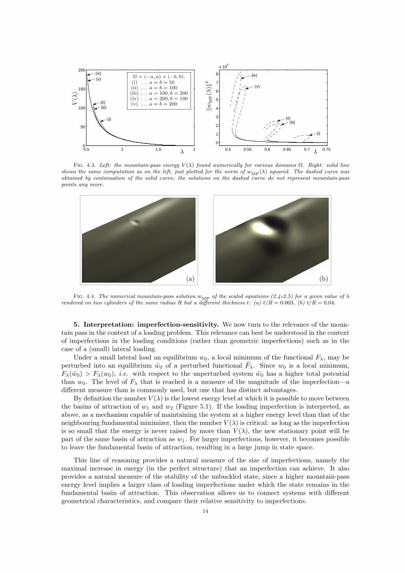
Figure 4.3 shows graphs of the mountain-pass energy V (λ,Ω) computed for various sizes ofdomain Ω. For each domain, the mountain-pass algorithm was employed to compute wMP forseveral values of λ. These mountain-pass solutions were then continued in λ using numericalcontinuation.

4.3. Influence of the domain. The localized nature of the solutions calculated above sug-gests that they should be independent of domain size, in the sense that for a sequence of domainsof increasing size the solutions converge (for instance pointwise on compact subsets). Such a con-vergence would also imply convergence of the associated energy levels. Similarly, we would expectthat the aspect ratio of the domain is of little importance in the limit of large domains.

We have tested these hypotheses by computing mountain-pass solutions on domains of differentsizes and aspect ratios. Generally solutions on different domains compare well; the maximaldifference in the second derivatives of w is two or three orders of magnitude smaller than thesupremum norm of the same derivative (the details of this comparison are given in [17]).

Here we only include a calculation of the mountain-pass energy level V (λ,Ω) for domains Ωof different aspect ratio and size (Figure 4.3).

The comparison of solutions computed on different domains and their respective energiessuggests that for each λ we are indeed dealing with a single, localized function defined on R2, ofwhich our computed solutions are finite-domain adaptations. In the rest of this paper we adoptthis point of view, and consequently we will write V (λ) instead of V (λ,Ω).

A consequence of this point of view is that dimples in cylinders with different geometricparameters are mapped to the same rescaled solution, or equivalently, that the same single-dimplesolution of (2.4-2.5) corresponds to differently-sized dimples on an actual cylinder, as a functionof the parameters (Figure 4.4).

13

0.5 1 1.5 20

50

100

150

200(iv) (v)

(ii) (iii)

(i)

0.5 0.55 0.6 0.65 0.7 0.75

0

1

2

3

4

5

6

7

8

x 105

(iv)

(v)

(ii) (iii)

(i)

Ω = (−a, a)× (−b, b):(i) . . . a = b = 50(ii) . . . a = b = 100(iii) . . . a = 100, b = 200(iv) . . . a = 200, b = 100(v) . . . a = b = 200V

(λ)

λ

‖wM

P(λ

)‖2

λ

Fig. 4.3. Left: the mountain-pass energy V (λ) found numerically for various domains Ω. Right: solid lineshows the same computation as on the left, just plotted for the norm of wMP(λ) squared. The dashed curve wasobtained by continuation of the solid curve; the solutions on the dashed curve do not represent mountain-passpoints any more.

(a) (b)

Fig. 4.4. The numerical mountain-pass solution wMP of the scaled equations (2.4-2.5) for a given value of λrendered on two cylinders of the same radius R but a different thickness t: (a) t/R = 0.003, (b) t/R = 0.04.

5. Interpretation: imperfection-sensitivity. We now turn to the relevance of the moun-tain pass in the context of a loading problem. This relevance can best be understood in the contextof imperfections in the loading conditions (rather than geometric imperfections) such as in thecase of a (small) lateral loading.

Under a small lateral load an equilibrium w0, a local minimum of the functional Fλ, may beperturbed into an equilibrium w0 of a perturbed functional Fλ. Since w0 is a local minimum,Fλ(w0) > Fλ(w0), i.e. with respect to the unperturbed system w0 has a higher total potentialthan w0. The level of Fλ that is reached is a measure of the magnitude of the imperfection—adifferent measure than is commonly used, but one that has distinct advantages.

By definition the number V (λ) is the lowest energy level at which it is possible to move betweenthe basins of attraction of w1 and w2 (Figure 5.1). If the loading imperfection is interpreted, asabove, as a mechanism capable of maintaining the system at a higher energy level than that of theneighbouring fundamental minimizer, then the number V (λ) is critical: as long as the imperfectionis so small that the energy is never raised by more than V (λ), the new stationary point will bepart of the same basin of attraction as w1. For larger imperfections, however, it becomes possibleto leave the fundamental basin of attraction, resulting in a large jump in state space.

This line of reasoning provides a natural measure of the size of imperfections, namely themaximal increase in energy (in the perfect structure) that an imperfection can achieve. It alsoprovides a natural measure of the stability of the unbuckled state, since a higher mountain-passenergy level implies a larger class of loading imperfections under which the state remains in thefundamental basin of attraction. This observation allows us to connect systems with differentgeometrical characteristics, and compare their relative sensitivity to imperfections.

14

V (λ)

w1

Fλ

w2

Fig. 5.1. In order to leave the basin of attraction of w1, the surplus energy should exceed V (λ)

5.1. Calibrating the mountain-pass energy. Comparing cylinders of varying geometryrequires a common measure of imperfection sensitivity. It is not a priori clear which measure totake; e.g., one might consider either the mountain-pass energy itself or the average spatial densityof this energy, which will result in different comparisons for cylinders of different wall volume.Here we choose to rescale the mountain-pass energy level by the other energy level present in theloaded cylinder: the energy that is stored in homogeneous compression of the unbuckled shell.

This calculation can be done in two slightly different ways. The first and most straightforwardis to rescale the dimensional mountain-pass energy (see (B.11) and (2.3))

64π6EtR2ε3V (λ) =Et4

8(3(1− ν2))3/2RV (λ),

by the elastic strain energy stored in the full length of the compressed cylinder of length L,

L

4πERtP 2 =

πt3EL

12(1− ν2)Rλ2,

to give an energy ratio, or a rescaled mountain-pass energy level,

α =1

2π√

3(1− ν2)t

L

V (λ)λ2

. (5.1)

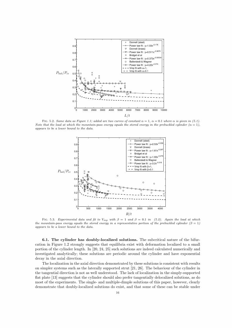
From this expression and the calculation shown in Figure 4.3 curves may be drawn in a plot ofload versus the ratio L/t (see Figure 5.2). Note that to obtain this figure from Figure 4.3 thecurve V (λ) was fitted to extend the range of λ. This figure shows two remarkable features:

1. The general trend of the constant-α curves is very similar to the trend of the experimentaldata;

2. The α = 1 curve, which indicates the load at which the mountain-pass energy equals thestored energy in the prebuckled cylinder, appears to be a lower bound to the data.

One may also consider an alternative way of rescaling energy. The cylinder is a long structure,and it is not clear to which extent the length of the structure is relevant for the imperfectionsensitivity. It may be reasonable to compare the energy of the mountain pass with the storedenergy contained in a representative section of the cylinder; the radius R provides a naturallength scale for such a representative section.

Similar to Figure 5.2, in Figure 5.3 we present curves of constant β, where β is the ratio ofmountain-pass energy to stored energy in a section of length 2πR:

β =1

4π2√

3(1− ν2)t

R

V (λ)λ2

. (5.2)

Once again to obtain Figure 5.3 we fitted V (λ) from Figure 4.3 to extend the range of λ.

6. Discussion and conclusions. The mathematical results and their interpretation in thecontext of a loading problem have brought a number of new and improved insights.

15

0 1000 2000 3000 4000 5000 6000 7000 8000 9000 100000

0.1

0.2

0.3

0.4

0.5

0.6

0.7

0.8

0.9

1Donnell (steel)Power law fit : y=1.03x−0.176

Donnell (brass)Power law fit : y=0.511x−0.0879

Bridget et alPower law fit : y=0.373x−0.00504

Ballerstedt & WagnerPower law fit : y=4.22x−0.374

Vmp fit with α=1,Vmp fit with α=0.1

Pfail/Pcr

L/t

Fig. 5.2. Same data as Figure 1.1; added are two curves of constant α = 1, α = 0.1 where α is given in (5.1).Note that the load at which the mountain-pass energy equals the stored energy in the prebuckled cylinder (α = 1),appears to be a lower bound to the data.

0 500 1000 1500 2000 2500 3000 3500 40000

0.1

0.2

0.3

0.4

0.5

0.6

0.7

0.8

0.9

1Donnell (steel)Power law fit : y=2.53x−0.358

Donnell (brass)Power law fit : y=1.61x−0.297

Bridget et alPower law fit : y=1.93x−0.279

Ballerstedt & WagnerPower law fit : y=3.2x−0.318

Vmp fit with β=1,Vmp fit with β=0.1

Pfail/Pcr

R/t

Fig. 5.3. Experimental data and fit to Vmp with β = 1 and β = 0.1 in (5.2). Again the load at whichthe mountain-pass energy equals the stored energy in a representative portion of the prebuckled cylinder (β = 1)appears to be a lower bound to the data.

6.1. The cylinder has doubly-localized solutions. The subcritical nature of the bifur-cation in Figure 1.2 strongly suggests that equilibria exist with deformation localized to a smallportion of the cylinder length. In [20, 24, 25] such solutions are indeed calculated numerically andinvestigated analytically; these solutions are periodic around the cylinder and have exponentialdecay in the axial direction.

The localization in the axial direction demonstrated by these solutions is consistent with resultson simpler systems such as the laterally supported strut [21, 26]. The behaviour of the cylinder inthe tangential direction is not as well understood. The lack of localization in the simply-supportedflat plate [13] suggests that the cylinder should also prefer tangentially delocalized solutions, as domost of the experiments. The single- and multiple-dimple solutions of this paper, however, clearlydemonstrate that doubly-localized solutions do exist, and that some of these can be stable under

16

constrained shortening.

6.2. The mountain pass is a single-dimple solution. The fact that the mountain-passsolution exists follows essentially from two features, the local minimality of the unbuckled stateand the existence of a large-deflection state of lower energy. The former is a simple consequence3

of the subcritical load level, but the latter is based on an essential property of the cylinder: fora sequence of cylinders for which R/t → ∞, the nondimensionalized load-carrying capacity (thehighest load at which the unbuckled state is not only a local but also a global energy minimizer)decreases to zero. This property was demonstrated implicitly by Hoff et al. [15], and Lemma 3.2provides a simplified proof of this result and a simple sequence of functions that illustrates theproperty.

However, the fact that the mountain-pass solution is localized, and even is the most localizedsolution that is possible—a single dimple—is interesting in its own right, and provides a comple-mentary view of the discussion of localization above. A different way of formulating this result isthat “creating the first dimple is the major obstacle”; afterwards one may increase the size of thedimple and add further dimples without ever returning to the same high energy level. In itselfthis interpretation points to a relationship between single dimples and imperfection sensitivity.

6.3. Single dimples in other contexts. Interestingly, single dimples have appeared in theliterature in a number of seemingly unrelated ways:

• In the celebrated high-speed camera images of Eßlinger [12] the first visible deformationis a single, well-developed dimple half-way between the ends of the cylinder. New dimplesquickly appear next to this first dimple, and the deformation then spreads around thecylinder and in axial direction. It is remarkable, though, that the first visible deformationis a single dimple.

• Some of the “worst” imperfections calculated by Deml and Wunderlich [9] and Wunderlichand Albertin [35] are in the form of a single dimple; as the load decreases, the dimplecontracts and becomes even more concentrated.

• Huhne et al. [19] assert that single dimples are also realistic and stimulating imperfectionsin the sense of [34].

• Zhu et al. [38] base their analysis of the scaling behaviour of the experimental bucklingload on the behaviour of a single dimple in other structural situations (the point-loadedcylinder and the sphere under uniform external pressure).

Note that the single-dimple appearances above are of three different types. Eßlinger’s dimpleis an experimental observation; the dimples of Wunderlich and co-workers and of Huhne et al. aregeometric imperfection profiles; and the dimples studied by Zhu et al. are only analogies, sincethey are solutions of different problems.

6.4. Scale-invariance of the localized solutions. It is an interesting observation thatthe Von Karman-Donnell-equations can be rescaled to depend only on the (rescaled) load level.For localized solutions, for which the boundary plays no role of importance, this implies that theset of solutions reduces to a one-parameter family. This allows for efficient computation of thebehaviour of such solutions but also gives interesting insight into the relationship between dimplesin cylinders of varying geometry (see e.g. Figure 4.4).

Naturally the scale-invariance is expected to break upon replacing the Von Karman-Donnell-equations by a different (probably more detailed) shell model. Nonetheless, it may reasonablybe expected that much of the understanding of the relationship between cylinders of differentgeometries remains roughly correct.

We certainly also expect that the large-scale geometry of the energy landscape does not dependon the specific model of the cylinder. Using a discrete mountain-pass algorithm to find mountain-pass points therefore does not depend on the Von Karman-Donnell-equations, and should givesimilar results regardless which shell model is used.

3On a finite domain this consequence is indeed simple; on an infinite domain it appears that besides thethird-order term also the fourth-order term in the energy has to be taken into account, as remarked in Section 3

17

6.5. Connection with sensitivity to imperfections and “Perturbation energy”.Kroplin and co-workers [23, 11, 32] were the first to suggest an estimate of the stability of theunbuckled state in terms of the ratio of a “perturbation energy” (Storenergie) to the pre-bucklingenergy. In early papers [23, 11] the perturbations are still fixed rather than determined, but fromboth the introduction and the final results in [32] it may be deduced that an optimization is doneover all perturbations (although this is simultaneously contradicted on page 333 of this paper).Unfortunately, these papers do not provide enough details to determine exactly what the authorscalculate.

There is one aspect in which our method can clearly be seen to differ from these earlierapproaches. The discrete mountain-pass algorithm takes into account global features of the energylandscape, and provides a global measure of the separation barrier between two states that liefar apart. This is different from the papers mentioned above, in which the method uses onlylocal information (reflected, for instance, in the assumption that the equilibria in question lie onthe same bifurcation branch). This difference is illustrated in Figure 6.1, where a local analysismight find stationary point w2, but the mountain-pass algorithm will find the more importantobstacle w4.

w1

w2

w3

w4

Fig. 6.1. While a local algorithm to find a critical point may settle on a minor critical point such as w3, themountain-pass algorithm, by its global setup, will converge on to the essential obstacle w4.

Appendix A. Proof of Lemma 3.2.Lemma 3.2 states that there exists a sequence of functions wδ, 1-periodic on R2, such that∫

[−1/2,1/2]2

w2δx ∼ 1,

∫[−1/2,1/2]2

∆w2δ = O(δ−1),

and∫

[−1/2,1/2]2

∆φ2δ = O(δ2−α) as δ → 0, (A.1)

for any α > 0. Here the function φδ solves equation (2.5) with periodic boundary conditions. Inaddition, wδ and φδ satisfy (2.6) on the boundary of [−1/2, 1/2]2.

The proof consists of three parts. In the first part we construct the functions wδ; in the secondpart we study the symmetry properties and the support of the right-hand side of (2.5); and in thethird part we show that this sequence has the asserted scaling.

A.1. Construction of wδ. Let fδ be given by

f ′′ε (s) =

14δ

dist(s,Z) < δ

0 otherwise,with fδ(0) = f ′δ(0) = 0.

Note that f is even and that f(1) = 1/4. Define

wδ(x, y) = fδ(y + x) + fδ(y − x)− 12fδ(2x)−

12y2.

18

0

0.5

1

1.5

2

–3 –2 –1 1 2 3

x

0

-0.2

-0.4

-0.6

y

0.6

0.4

0.2

0

-0.2

-0.4

-0.6

x

0.60.4

0.20

-0.2-0.4

-0.6

Fig. A.1. The functions f and −w; on the right the plotting area is slightly larger than one period.

We shall drop the subscript δ and simply write w and f .The function w is periodic on R2 with period 1 in each direction. To show this, we prove that

the first two derivatives match up on opposite sides of [−1/2, 1/2]× [−1/2, 1/2]:• By the symmetry of f the function w is even in both x and y. Consequently w takes the

same values on (1/2, y) and (−1/2, y); the same holds for (x,±1/2).• For the comparison of the first derivatives we calculate∫ 1/2

−1/2

wxx(x, y) dx =∫ 1/2

−1/2

f ′′(y + x) dx+∫ 1/2

−1/2

f ′′(y − x) dx− 2∫ 1/2

−1/2

f ′′(2x) dx = 0,

implying that wx(−1/2, y) = wx(1/2, y); by the symmetry of w it follows that wx(−1/2, y) =wx(1/2, y) = 0. Similarly, using the definition of fδ we find that∫ 1/2

−1/2

wyy(x, y) dy =∫ 1/2

−1/2

f ′′(y + x) dy +∫ 1/2

−1/2

f ′′(y − x) dy − 1 = 0,

implying that wy(x,−1/2) = wy(x, 1/2) = 0.Periodicity on R2 then follows from the remark that all second derivatives of w are periodic withperiod 1 in x and y.

A.2. Support, symmetry, and boundary conditions. Next we investigate the right-hand side of (2.5). We find

[w,w] + wxx =(f ′′(y + x) + f ′′(y − x)− 2f ′′(2x))(f ′′(y + x) + f ′′(y − x)− 1)

− (f ′′(y + x)− f ′′(y − x))2

+ (f ′′(y + x) + f ′′(y − x)− 2f ′′(2x))= 4f ′′(y + x)f ′′(y − x)− 2f ′′(2x)(f ′′(y + x) + f ′′(y − x)).

This expression has zero integral over [−1/2, 1/2]2. This follows from the periodicity of w:∫ 1/2

−1/2

∫ 1/2

−1/2

wxxwyy dxdy =∫ 1/2

−1/2

∫ 1/2

−1/2

w2xy dxdy (A.2)

by partial integration. More is true, however; we analyse the support of [w,w]+wxx in [−1/2, 1/2]2

in more detail.The value of f ′′ is either (4δ)−1 or zero; in order to determine [w,w] + wxx it is therefore

sufficient to calculate the measures of the pairwise intersections of the supports of f ′′(y + x),f ′′(y − x), and f ′′(2x):

• The intersection of the supports of f ′′(y + x) and f ′′(y − x) has total area 4δ2 (seeFigure A.2).

• The intersection of the supports of f ′′(y + x) and f ′′(2x) also has total area 4δ2 (seeFigure A.3).

19

2δ

y = −1

2y =

1

2

x = −1

2

x =1

2

Fig. A.2. The areas of the black regions add up to 4δ2

δ

Fig. A.3. The areas of the black regions add up to 4δ2

Since the support of [w,w]+wxx concentrates onto a discrete set of points, let us examine thebehaviour at one of these points. For small δ the support forms disjoint sets in [−1/2, 1/2]2, andwe can restrict our attention to the origin alone.

If |s| < 1/2, then f ′′δ (s) can be written as

f ′′δ (s) =1δg(sδ

),

where

g(σ) =

14

|σ| < 1

0 otherwise.

Therefore, as long as |(x, y)| < 1/4,

4f ′′δ (y + x)f ′′δ (y − x)− 2f ′′δ (2x)(f ′′δ (y + x) + f ′′δ (y − x)) =

=4δ2g

(y + x

δ

)g

(y − x

δ

)− 2δ2g

(2xδ

)[g

(y + x

δ

)+ g

(y − x

δ

)]=

1δ2F(δ−1(x, y)

), (A.3)

where we introduce a new function F , which does not depend on δ, to summarize the line above.Note that suppF ⊂ [−2, 2]2. Note also that by (A.2) the function F has zero integral; in addition,

20

since f ′′δ is even, the function 4f ′′δ (y + x)f ′′δ (y − x)− 2f ′′δ (2x)(f ′′δ (y + x) + f ′′δ (y − x)) is also evenin x and in y. Therefore ∫

R2xF((x, y)

)dxdy =

∫R2yF((x, y)

)dxdy = 0.

This property will be used below.

The assertion also states that the functions w and φ satisfy (2.6) on the boundary of [−1/2, 1/2]2.We first note that w and φ are periodic in the following sense:

w(x± 1/2, y ± 1/2) = w(x, y) and φ(x± 1/2, y ± 1/2) = φ(x, y). (A.4)

For w this is a simple consequence of the functional form of w; for φ it is a consequence of theuniqueness of solutions of (2.5) under periodic boundary conditions. The periodicity of w and φ inthe y-direction in (2.6) then follows from a repeated application of (A.4). Similarly, the symmetryconditions in x in (2.6) follow from a combination of the symmetry of w and φ around y = 0 incombination with (A.4).

A.3. Scaling properties. We now use the information gathered above to show that thesequence wδ has the scaling properties of (A.1). All function spaces are on [−1/2, 1/2]2.

First, f ′δ remains bounded on bounded sets as δ → 0; therefore∫Ωw2

δx converges to a finite,positive value. In addition, all second derivatives of wδ remain bounded in L1, so that

‖∆wδ‖L1 ≤ C.

The second derivative f ′′δ is bounded by 1/4δ, so that we can estimate

‖∆wδ‖2L2 ≤ ‖∆wδ‖L1 ‖∆wδ‖L∞ ≤ C

δ.

Turning to φδ, we start by remarking that [wδ, wδ] + wδxx is bounded in L1, since∫|(x,y)|<1/4

∣∣[wδ, wδ] + wδxx

∣∣ = 1δ2

∫|(x,y)|<2δ

∣∣F (δ−1(x, y))∣∣ = O(1).

Since W 2,p → L∞ for all p > 1, the solution of

∆2ψ = h

satisfies

‖∆ψ‖Lp′ = supζ

∫Ω

∆ψ∆ζ‖∆ζ‖Lp

= supζ

∫Ωhζ

‖∆ζ‖Lp

≤ C ‖h‖L1

‖ζ‖L∞

‖ζ‖W 2,p

≤ C ‖h‖L1 ,

so that

‖φδ‖W 2,p′ ≤ C ‖[wδ, wδ] + wδxx‖L1 ≤ C,

where 1/p+ 1/p′ = 1. Using W 2,p′ → C1,1−2/p′ we find

‖φδ‖C1,1−2/p′ ≤ C ‖φδ‖W 2,p′ ≤ C.

Writing, locally at the origin,

φδ(x, y) = φδ(0, 0) +∇φδ(0, 0) · (x, y) +O(|(x, y)|2(1−1/p′))

,

21

we find by multiplying the equation (2.5) by φδ and integrating,

‖∆φδ‖2L2([−1/2,1/2]2) = 2∫

[−1/4,1/4]2φδ

[wδ, wδ] + wδxx

= 2

φδ(0, 0)δ2

∫[−1/4,1/4]2

F(δ−1(x, y)

)+ 2

∇φδ(0, 0)δ2

·∫

[−1/4,1/4]2(x, y)F

(δ−1(x, y)

)+O

(δ2(1−1/p′)

)= O

(δ2(1−1/p′)

),

since the zeroth and first moments of F are zero. Since p′ may be chosen arbitrary large, thisestimate concludes the proof.

Appendix B. Derivation of the Von Karman-Donnell equations.The common aim of the many elastic shell theories is to approximate three-dimensional elas-

ticity by a reduced description in which the unknowns are functions of not three but two spatialvariables, see for example [6]. For the Von Karman-Donnell cylinder the central approximationis the director Ansatz, which states that a normal to the centre surface remains normal throughdeformation. By this Ansatz the displacement is fully characterized by the displacement vector(u, v, w), a function of the two in-plane spatial variables x and y, where u is the displacementin axial (x-), v in tangential (y-), and w in the radial direction. Apart from some rescaling thefunction w is the same as the unknown w in the rest of this paper.

In the formulation of Section 2 the unknowns u and v are replaced by the Airy stress function φ,which is derived by minimization with respect to the displacements u and v for fixed w. Thisminimization argument is well known in the context of the Von Karman plate theory and canbe found in many textbooks. Determining the boundary conditions that the function φ satisfies,however, is not straightforward (see also the discussion in [27]), and it is for this reason that wenow describe the argument in detail. The main goal is to show that the function φ is periodic inthe tangential direction.

B.1. Energy and shortening. All quantities in this appendix are dimensional. We assumea cylinder of thickness t, length L, and radius R, and we set Ω = [0, L] × [0, 2πR]. The storedenergy given by [31] is

E1 =t3E

24(1− ν2)

∫Ω

∆w2 +t

2E

∫Ω

[(σ11 + σ22)2 − 2(1 + ν)(σ11σ22 − σ2

12)]

for a linear material of Young’s modulus E and Possion’s ratio ν. Under the assumption of planestress the stress and strain tensors are related by

σ =E

1− ν2

[(1− ν)ε+ ν tr ε I

]=

E

1− ν2

(ε11 + νε22 (1− ν)ε12(1− ν)ε12 ε22 + νε11

), (B.1)

and under the small-angle approximation the strain tensor can be expressed in the displacementsas

ε =

(ux + 1

2w2x

12uy + 1

2vx + 12wxwy

12uy + 1

2vx + 12wxwy vy + 1

2w2y − ρw

). (B.2)

These choices for the energy and for the stress and strain tensors are very similar to those for aflat plate. The intrinsic curvature of the cylinder, of magnitude ρ = 1/R, only appears in the lastterm of ε22, −ρw, which expresses the fact that radial displacement creates extensional strain inthe y-direction.

22

The average axial shortening is given by

S1 = − 12πR

∫ 2πR

0

[u(L, y)− u(0, y)

]dy = − 1

2πR

∫Ω

ux dxdy,

and an equilibrium (u, v, w) at load level P is a stationary point of the total potential V1 =E1 − PS1.

B.2. Boundary conditions. At the boundaries y = 0, 2πR it is natural to assume that u,v, and w are periodic, but at x = 0, L there is a certain amount of choice.

The boundary conditions on w (see (2.6a)) are

wx = (∆w)x = 0, at x = 0, L, (B.3)

and these conditions signify a fixed angle (wx = 0) and zero radial force ((∆w)x = 0). They mayalso be understood as symmetry boundary conditions, as in the case of a sequence of cylindersstacked on top of each other. For u and v we assume boundary conditions

uy = 0 and σ12 = 0, at x = 0, L, (B.4)

which signify that the ends of the cylinder are rigid in the x-direction and that there is no frictionbetween the cylinder and the apparatus holding it. Note that the pair of boundary conditionsσ12 = 0 and (∆w)x = 0 together states that the loading apparatus exerts only axial forces on thecylinder.

The boundary conditions on w are invariant under addition of a constant to w, i.e. underreplacing w by w + c; for stationary points we may exploit this fact.

Lemma B.1. If (u, v, w) is a stationary point of E1 − PS1 under boundary conditions (B.3-B.4), then ∫

Ω

σ22 = 0. (B.5)

Proof. Under the replacement w 7→ w + c, we have

dσ

dc= − Eρ

1− ν2

(ν 00 1

),

and therefore

0 =d

dc(E1 − PS1) = − tρ

1− ν2

∫Ω

[(σ11 + σ22)(ν + 1)− (1 + ν)(σ11 + νσ22)

]= −tρ

∫Ω

σ22.

B.3. Derivation of the Airy stress function φ. The energy (2.7) and the Airy stressfunction φ are derived from the total potential E1 − PS1 by minimization with respect to thedisplacements u and v for fixed w. Performing this minimization on the second term in E1 yieldsthe classical plate equilibrium equations

σ11x + σ12y = 0 and σ12x + σ22y = 0.

Note that the derivative of S1 with respect to u only creates boundary terms. By applying threetimes the well-known characterization of divergence-free vector fields as rotations of scalar fields(see e.g. [3, Th. XII.3.5]) we obtain the local existence of a function φ satisfying

σ11 = Eφyy, σ12 = −Eφxy, and σ22 = Eφxx, (B.6)

where we use the traditional scaling of φ by Young’s modulus.23

B.4. Boundary conditions on φ. The existence of the function φ is the result of a localdifferential-geometric argument, and as such gives no reason for φ to be periodic in y. The followingtheorem shows that after a normalization transformation the function φ can indeed be assumedto be periodic in y, and may be taken to satisfy the same boundary conditions as the function w.

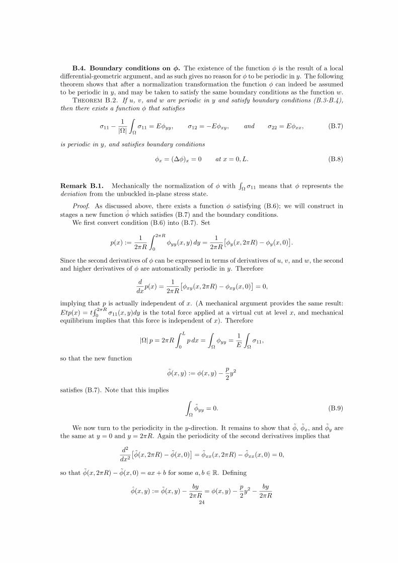
Theorem B.2. If u, v, and w are periodic in y and satisfy boundary conditions (B.3-B.4),then there exists a function φ that satisfies

σ11 −1|Ω|

∫Ω

σ11 = Eφyy, σ12 = −Eφxy, and σ22 = Eφxx, (B.7)

is periodic in y, and satisfies boundary conditions

φx = (∆φ)x = 0 at x = 0, L. (B.8)

Remark B.1. Mechanically the normalization of φ with∫Ωσ11 means that φ represents the

deviation from the unbuckled in-plane stress state.

Proof. As discussed above, there exists a function φ satisfying (B.6); we will construct instages a new function φ which satisfies (B.7) and the boundary conditions.

We first convert condition (B.6) into (B.7). Set

p(x) :=1

2πR

∫ 2πR

0

φyy(x, y) dy =1

2πR[φy(x, 2πR)− φy(x, 0)

].

Since the second derivatives of φ can be expressed in terms of derivatives of u, v, and w, the secondand higher derivatives of φ are automatically periodic in y. Therefore

d

dxp(x) =

12πR

[φxy(x, 2πR)− φxy(x, 0)

]= 0,

implying that p is actually independent of x. (A mechanical argument provides the same result:Etp(x) = t−

∫ 2πR

0σ11(x, y)dy is the total force applied at a virtual cut at level x, and mechanical

equilibrium implies that this force is independent of x). Therefore

|Ω| p = 2πR∫ L

0

p dx =∫

Ω

φyy =1E

∫Ω

σ11,

so that the new function

φ(x, y) := φ(x, y)− p

2y2

satisfies (B.7). Note that this implies ∫Ω

φyy = 0. (B.9)

We now turn to the periodicity in the y-direction. It remains to show that φ, φx, and φy arethe same at y = 0 and y = 2πR. Again the periodicity of the second derivatives implies that

d2

dx2

[φ(x, 2πR)− φ(x, 0)

]= φxx(x, 2πR)− φxx(x, 0) = 0,

so that φ(x, 2πR)− φ(x, 0) = ax+ b for some a, b ∈ R. Defining

φ(x, y) := φ(x, y)− by

2πR= φ(x, y)− p

2y2 − by

2πR24

the function φ still satisfies (B.7), and

φ(x, 2πR)− φ(x, 0) = ax.

Finally, we find that

a = φx(0, 2πR)− φx(0, 0) =∫ 2πR

0

φxy(0, y) dy =1E

∫ 2πR

0

σ12(0, y) dy(B.4)= 0,

and therefore that φ(x, 2πR) − φ(x, 0) = 0 for all x. The same follows for φx(x, 2πR) − φx(x, 0)by differentiation.

To show that φy also matches,

d

dx

[φy(x, 2πR)− φy(x, 0)

]=[φxy(x, 2πR)− φxy(x, 0)

]= 0,

and therefore φy(x, 2πR) − φy(x, 0) is constant in x; by (B.9) this constant is zero. This provesthat φ satisfies (B.7) and is periodic in y.

We finally discuss the boundary conditions at x = 0, L, and we follow the line of reasoningof [27]. By (B.4) and (B.1) ε12 = 0 at x = 0, L, so that by (B.3) and (B.4)

vxy =∂

∂y(2ε12 − uy − wxwy) = 0 at x = 0, L.

Therefore

ε22x = vxy + wywxy − ρwx(B.4)= 0 at x = 0, L.

Using Eε22 = σ22 − νσ11, we then find

φxxx − νφxyy = φxxx − νφxyy =1E

d

dx(σ22 − νσ11) = ε22x = 0,

and by adding (1 + ν)φxyy = −(1/E)(1 + ν)σ12y = 0 it follows that

(∆φ)x = φxxx + φxyy = 0 at x = 0, L,

which proves one part of (B.8).From φxy = −σ12/E = 0 we find that

φx(0, y) = c0 and φx(L, y) = cL for all y ∈ [0, 2πR].

Writing

2πR(cL − c0) =∫

Ω

φxx =1E

∫Ω

σ22(B.5)= 0

we find that cL = c0. Now the function

φ(x, y) := φ(x, y)− c0x = φ(x, y)− p

2y2 − by

2πR− c0x

satisfies (B.7) and (B.8) and is periodic in y. This concludes the proof.

Remark B.2. It is instructive to note that the periodicity of φ is a result of the specific choiceof boundary conditions, and will in fact not hold if different boundary conditions are taken. Forinstance, if a tangential shear stress τ is applied at the cylinder ends (i.e. the cylinder is loadedunder torsion), then the coefficient a in the derivation above will not vanish, and φx will not beperiodic in y.

25

B.5. Putting it all together. By an elementary but lengthy calculation we find that φ, asprovided by Theorem B.2, satisfies the equation

∆2φ+ ρwxx + [w,w] = 0 in Ω, (B.10)

and that the second term in E1 can be written as

tE

2

∫Ω

[∆φ2 − 2(1 + ν)[φ, φ]

].

By the boundary conditions given by Theorem B.2 the second term vanishes, and the total storedenergy functional can therefore be written as

E2(w) :=t3E

24(1− ν2)

∫Ω

∆w2 +tE

2

∫Ω

∆φ2.

Note that this energy is a function of w alone; the function φ in this definition is assumed to begiven by (B.10), with the boundary conditions of Theorem B.2. Similarly, we rewrite the averageshortening as

S2(w) := S1(u) = − 12πR

∫Ω

ux

(B.2)= − 1

2πR

∫Ω

[ε11 − 1

2w2x

](B.1)= − 1

2πRE

∫Ω

[σ11 − νσ22

]+

14πR

∫Ω

w2x

(B.7)= − 1

2πR

∫Ω

[φyy − νφxx

]+

14πR

∫Ω

w2x

=1

4πR

∫Ω

w2x.

A stationary point w of E2 − PS2 satisfies the Euler equation

t2

12(1− ν2)∆2w +

P

2πREtwxx − ρφxx − 2[w, φ] = 0,

where again φ is related to w by (B.10). With the nondimensionalization

w = 4π2Rw, φ = 16π4R2 φ, x 7→ 2πRx, y 7→ 2πR y,

we then obtain equations (2.4) and (2.5), and the dimensional energy E2 and average shorteningS2 above can be expressed in these variables as

E2 =π2t3E

6(1− ν2)

∫∆w2 + 32π6tER2

∫∆φ

2, S2 = 4π3R

∫w2

x. (B.11)

REFERENCES

[1] B. O. Almroth, Postbuckling behaviour of axially compressed circular cylinders, AIAA J., 1 (1963), pp. 627–633.

[2] A. Ambrosetti and P. H. Rabinowitz, Dual variational methods in critical point theory and applications,J. Functional Analysis, 14 (1973), pp. 349–381.

[3] S. S. Antman, Nonlinear problems of elasticity, vol. 107 of Applied Mathematical Sciences, Springer, NewYork, second ed., 2005.

[4] J. Arbocz and C. D. Babcock, The effect of general imperfections on the buckling of cylindrical shells,ASME J. Appl. Mech., 36 (1969), pp. 28–38.

[5] W. Ballerstedt and H. Wagner, Versuche uber die Festigkeit dunner unversteifter Zylinderunter Schub-und Langskraften, Luftfahrtforschung, 13 (1936), pp. 309–312.

26

[6] Z. P. Bazant and L. Cedolin, Stability of structures: elastic, inelastic, fracture and damage theories,O.U.P., 1991. ISBN 0-19-5055529-2.

[7] F. J. Bridget, C. C. Jerome, and A. B. Vosseller, Some new experiments on buckling of thin-wallconstruction, Trans. ASME Aero. Eng., 56 (1934), pp. 569–578.

[8] Y. S. Choi and P. J. McKenna, A mountain pass method for the numerical solution of semilinear ellipticproblems, Nonlinear Anal., 20 (1993), pp. 417–437.

[9] M. Deml and W. Wunderlich, Direct evaluation of the worst imperfection shape in shell buckling, Comput.Methods Appl. Mech. Engrg., 149 (1997), pp. 201–222.

[10] L. H. Donnell, A new theory for buckling of thin cylinders under axial compression and bending, Trans.ASME Aero. Eng., AER-56-12 (1934), pp. 795–806.

[11] H. Duddeck, B. Kroplin, D. Dinkler, J. Hillmann, and W. Wagenhuber, Non linear computations inCivil Engineering Structures (in German), in DFG Colloquium, 2-3 March 1989, Springer Verlag, 1989.

[12] M. Eßlinger, Hochgeschwindigkeitsaufnahmen vom Beulvorgang dunnwandiger, axialbelasteter Zylinder,Der Stahlbau, 39 (1970), pp. 73–76.

[13] P. R. Everall and G. W. Hunt, Mode jumping in the buckling of struts and plates: a comparative study,Int. J. Non-Linear Mech., 35 (2000), pp. 1067–1079.

[14] D. J. Gorman and R. M. Evan-Iwanowski, An analytical and experimental investigation of the effects oflarge prebuckling deformations on the buckling of clamped thin-walled circular cylindrical shells subjectedto axial loading and internal pressure, Develop. in Theor. and Appl. Mech., 4 (1970), pp. 415–426.

[15] N. Hoff, W. Madsen, and J. Mayers, Post-buckling equilibrium of axially compressed circular cylindricalshells, AIAA J., 4 (1966), pp. 126–133.

[16] J. Horak, Constrained mountain pass algorithm for the numerical solution of semilinear elliptic problems.To appear in Numerische Mathematik.

[17] J. Horak, G. J. Lord, and M. A. Peletier, Application of the numerical mountain-pass algorithm tocylinder buckling. in preparation.

[18] J. Horak and P. J. McKenna, Traveling waves in nonlinearly supported beams and plates, in Nonlinearequations: methods, models and applications (Bergamo, 2001), vol. 54 of Progr. Nonlinear DifferentialEquations Appl., Birkhauser, Basel, 2003, pp. 197–215.

[19] C. Huhne, R. Zimmerman, R. Rolfes, and B. Geier, Sensitivities to geometrical and loading imperfectionson buckling of composite cylindrical shells, in Proceedings European Conference on Spacecraft Structures,Materials and Mechanical Testing, Toulouse, 2002.

[20] G. W. Hunt and E. Lucena Neto, Localized buckling in long axially-loaded cylindrical shells, J. Mech. Phys.Solids, 39 (1991), pp. 881–894.

[21] G. W. Hunt, M. A. Peletier, A. R. Champneys, P. D. Woods, M. A. Wadee, C. J. Budd, and G. J.Lord, Cellular buckling in long structures, Nonlinear Dynamics, 21 (2000), pp. 3–29.

[22] W. T. Koiter, On the stability of elastic equilibrium, PhD thesis, Technische Hogeschool, Delft (TechnologicalUniversity of Delft), Holland, 1945. English translation issued as NASA, Tech. Trans., F 10, 833, 1967.

[23] B. Kroplin, D. Dinkler, and J. Hillmann, An energy perturbation method applied to non linear structuralanalysis, Comput. Methods Appl. Engrg., 52 (1985), pp. 885–897.

[24] G. J. Lord, A. R. Champneys, and G. W. Hunt, Computation of localized post buckling in long axially-compressed cylindrical shells, in Localization and Solitary Waves in Solid Mechanics, A. R. Champneys,G. W. Hunt, and J. M. T. Thompson, eds., vol. A 355, Special Issue of Phil. Trans. R. Soc. Lond, 1997,pp. 2137–2150.

[25] , Computation of homoclinic orbits in partial differential equations: an application to cylindrical shellbuckling, SIAM J. Sci. Comp., 21 (1999), pp. 591–619.

[26] M. A. Peletier, Sequential buckling: A variational analysis, SIAM J. Math. Anal., 32 (2001), pp. 1142–1168.[27] D. Schaeffer and M. Golubitsky, Boundary conditions and mode jumping in the buckling of a rectangular

plate, Commun. Math. Phys., 69 (1979), pp. 209–236.[28] D. Smets and G. J. B. van den Berg, Homoclinic solutions for Swift-Hohenberg and suspension bridge type

equations, J. Diff. Eqns., 184 (2002), pp. 78–96.[29] M. Struwe, Variational Methods, Springer Verlag, 1990.[30] R. C. Tennyson, An experimental investigation of the buckling of circular cylindrical shells in axial com-

pression using the photoelastic technique, Tech. Rep. 102, University of Toronto, 1964.[31] T. von Karman and H. S. Tsien, The buckling of thin cylindrical shells under axial compression, Journal

of the Aeronautical Sciences, 8 (1941), pp. 303–312.[32] W. Wagenhuber and H. Duddeck, Numerischer Stabilitatsnachweis dunner Schalen mit dem Konzept der

Storenergie, Archive of Applied Mechanics, 61 (1991), pp. 327–343.[33] V. I. Weingarten, E. J. Morgan, and P. Seide, Elastic stability of thin-walled cylindrical and conical shells

under axial compression, AIAA J., 3 (1965), pp. 500–505.[34] T. A. Winterstetter and H. Schmidt, Stability of circular cylindrical steel shells under combined loading,

Thin-Walled Structures, 40 (2002), pp. 893–909.[35] W. Wunderlich and U. Albertin, Analysis and load carrying behaviour of imperfection sensitive shells,

Int. J. Numer. Meth. Engng., 47 (2000), pp. 255–273.[36] N. Yamaki, Elastic Stability of Circular Cylindrical Shells, vol. 27 of Applied Mathematics and Mechanics,

Elsevier, 1984.[37] Y. Yoshimura, On the mechanism of buckling of a circular shell under axial compression, Tech. Rep. 1390,

NACA, 1955. Sec 7.7.

27

[38] E. Zhu, P. Mandal, and C. R. Calladine, Buckling of thin cylindrical shells: an attempt to resolve aparadox, Int. J. Mechanical Sciences, 44 (2002), pp. 1583–1601.

28