
CYCLE TIME REDUCTION AND STRATEGIC INVENTORY PLACEMENT …web.mit.edu/~sgraves/www/hetzel93.pdf ·...
106
Cycle Time Reduction and Strategic Inventory Placement Across a Multistage Process by William B. Hetzel B.S. Chemistry – Yale University (1988) Submitted to the Sloan School of Management and the Department of Chemical Engineering In Partial Fulfillment of the Requirements for the Degrees of Master of Science in Management and Master of Science in Chemical Engineering in conjunction with the Leaders for Manufacturing Program at the Massachusetts Institute of Technology June 1993 @ 1993 Massachusetts Institute of Technology n -Z@ #!Jg.?j \ Signature of Author_ ) ’ MIT Sloan School O NVlanagement MIT Department of Chemical Engineering May 1993 Certiilled by ~.~~ / Stephen C. Graves Professor of Management Science 5 dtiq>?.~ ‘ Certified by ~-–Ged&e Stephan%poulos Arthur D. Little Professor of Chemical Engineering Accepted by Jeffrey A. Barks Associate Dean, Sloan Master’s and Bachelor’s Programs 1
Transcript of CYCLE TIME REDUCTION AND STRATEGIC INVENTORY PLACEMENT …web.mit.edu/~sgraves/www/hetzel93.pdf ·...
Cycle Time Reduction and Strategic Inventory PlacementAcross a Multistage Process
by
William B. HetzelB.S. Chemistry – Yale University (1988)
Submitted to the Sloan School of Managementand the Department of Chemical Engineering
In Partial Fulfillment of the Requirements for the Degrees of
Master of Science in Managementand
Master of Science in Chemical Engineering
in conjunction with theLeaders for Manufacturing Program
at theMassachusetts Institute of Technology
June 1993
@ 1993 Massachusetts Institute of Technology
n-Z@ #!Jg.?j\Signature of Author_ ) ’
MIT Sloan School O NVlanagementMIT Department of Chemical Engineering
May 1993
Certiilled by~.~~
/ Stephen C. GravesProfessor of Management Science
5dtiq>?.~ ‘
Certified by~-–Ged&e Stephan%poulos
Arthur D. Little Professor of Chemical Engineering
Accepted byJeffrey A. Barks
Associate Dean, Sloan Master’s and Bachelor’s Programs
1


Cycle Time Reduction and Strategic Inventory PlacementAcross a Multistage Process
by
William B. Hetzel
Submitted to the Sloan School of Management and the Department of ChemicalEngineering in Partial Fulfillment of the Requirements for the Degrees of
Master of Science in Management andMaster of Science in Chemical Engineering
ABSTRACT
This thesis project examines cycle time and inventory reduction, which are centralthrusts of Eastman Kodak’s corporate strategy. The project shows that these reductionefforts cannot be addressed in isolation. Instead, they represent the outcome that resultsfrom improving the fundamental manufacturing processes across the supply chain.
Through a series of three case studies, the project applies academic models to realsituations at the Eastman Kodak Company. The models quantify the relationshipsbetween cycle time and inventory reduction and the following manufacturing processissues:
● setup timeQ product sequencing● supply and demand variability● supply chain structure● customer service
The case studies build in scope from a detailed examination of one product in onemanufacturing stage to a high level view across the entire film supply chain.
The first case study develops a specific lot size and inventory strategy at theproduct level. It quantifies and prioritizes setup time improvements and processvariability reductions.
The second case study extends the analysis to the machine level for multipleproducts. It incorporates capacity constraints and product sequencing issues critical toKodak’s manufacturing processes.
The third case study covers the entire film supply chain. It determines where theminimum safety stocks can be placed at each stage to attain a desired level of customerservice. It also addresses supply chain issues of information flow and asset utilization.
The thesis project ultimately develops a strategy and quantifies the benefits forcycle time and inventory reduction at three levels of detail. It demonstrates the value ofbroadening the scope of analysis to cover the entire supply chain. Together, the threecase studies provide an annual savings potential up to $7 MM.
Thesis Advisors:Anthony L. Spatorico, Eastman Kodak CompanyProfessor Stephen C. Graves, MIT Sloan School of ManagementProfessor George Stephanopoulos, MT Departmen.f of Chemical En.gin.eerin.g
3

ACKNOWLEDGMENTS
I would like to thank all the people at Kodak who welcomed me with suchenthusiasm and encouragement. Special thanks go to my advisors Tony Spatorico atKodak and Steve Graves and George Stephanopoulos at MIT for their support andguidance. Many people at Kodak provided tremendous assistance and resources: TimCikmo, George Daddis, Ed Hoffman, Andy Piot.rowski, Bill Poole, Laurie Stefanski, theRoll Coating Division, the Black & White team, the HSD team, and the SCOT team,
I gratefully acknowledge the support and resources made available to me throughthe Leader For Manufacturing Program, a partnership between MIT and major U.S.manufacturing companies.
Finally my deepest appreciation to my wife Jennifer for accompanying me inperson and in spirit during this experience.

TABLE OF C0NTENTf3
Chapter L1.1.1.2.1.3.
Chapter II.II. 1.11.2.11.3.11.4.
Chapter III.III. 1.111.2.111.3.111.4.
Chapter IV.IV.1 ~IV.2.IV.3.IV.4.lv.5.IV.6.N.7.
Chapter V.V.1.V.2.V.3.
Chapter VI.VI.1.VL2.VL3.
Chapter VII.
Title Page . . . . . . . . . . . . . . . . . . . . . . . . . . . . . . ...0.. . . . . . . . . . . . . . . . . . . . . . . . . . . . . . . . . . . . . . . . . . . . . . . . . . . 1Abstract . . . . . . . . . . . . . . . . . . . . . ...*... . . . . . . . . . . . . . . . . . . . . . . . . . . . . . . . . . . . . . . . . . . ● . . . . . . . . . . . . . . . . . . 3Acknowledgments . . . . . . . . . . . . . . . . . . . . . . . . . . . . . . . . . . . . . . . . . . . . . . . . . . . . . . . . . . . . . . . . . . . . . . . . 4Table of Contents . . . . . . . . . . . . . . . . . ...*... . . . . . . . . . . . . . . . . . . . . . . . .. . . . . . . . . . . . . . . . . . . . . . . . . ., 5List of Figures . . . . . . . . . . . . . . . . . . . . . . . . . . . . . . . . . . . . . . . . . . . . . . . . . . . . . . . . . . . . . . . . . . . . . . . . . . . . . . . 6List of Tables . . . . . . . . . . . . . . . . . . . . . . . . . . . . . . . . . . . . . . . . ...>.... . . . . . . . . . . . . . . . . . . . . . . . . . . . . . . . .7
IntroductionValue of Cycle Time Reduction . . . . . . . . . . . . . . . . . . . . . . . . . . . . . . . . . . . . . . . . . . . . . . . . . . . 8Industry Background . . . . . . . . . . . . . . . . . . . . . . . . . . . . . . . . . . . . . . . . . . . . . . . .. . . . . . . . . . . . . . . . . . . . 13Thesis Overview . . . . . . . . . . . . . . . . . . . . . . . . . . . . . . . . . . ...>.... . . . . . . . . . . . . . . . . . . . . . . . . . . . . . . . . .21
Single Product AnalysisGoals . . . . . . . . . . . . . . . . . . . . . . . . . . . . . . . . . . . . . . . . . . . . . . . . . . . . . . . . . . . . . . . . . . . . . . . . . . . . . . . . . . . . ● . . . . . . . . 25Methodology . . . . . . . ...*. . . . . . . . . . . . . . . . . . . . . . . . . . . . . . . . . . . . . . . . . . . . . . . . . . . . . . . . . . . . . . . . . . . . . . 27Results . . . . . . . . . . . . . . . . . ...*... . . . . . . . . . . . . . . . . . . . . . . . . . . . . . . . . . . . . . . . . . . . . . . . . . . . . . . . . . . . . . . . . . . . 30Implementation . . . ...*..... . . . . . . . . . . . . . . . . . . . . . . . . . . . . . . . . . . . . . . . . . . . . . . . . . . . . . . . . . . . . . . . . .38
Single Machine AnalysisGoals . . . . . . . . . . . . . . . . . . . . . . . . . . . . . . . . . . . . . . . . . . . . . . . . . . . . . . . . . . . . . . . . . . . . . . . . . . . . . . . . . . . . . . . . . . . . . 41Methodology . . . . . . . . . . . . . . . . . . . . . . . . . . . . . . . . . . . . . . . . . . . . . . . . . . . ...*..... . . . . . . . . . . . . . . . . . . . . .42Results . . . . . . . . . . . . . . . . . . . . . . . . . . . . . . . . . . . . . . . . . . . . . . . . . . . . . . . . . . . . . . . . . . . . . . . . . . . . . . . . . . . . . . . . . . . 45Implementation . . . . . . . . . . . . . . . . . . . . . . . . . . . ..*...... . . . . . . . . . . . . . . . . . . . . . . . . . . . . . . . . . . . . . . . . .48
Supply Chain AnalysisGoals . . . . . . . . . . . . . . . . . . . . . . . . . . . . . . ...*.. . . . . . . . . . . . . . . . . . . . . . . . . . . . . . . . . . . . . . . . . . . . . . . . . . . . . ...*.51Methodology . . . . . . . . . . . . . . . . . . . . . . . . . . . . . . . . . . . . . . . . . . . . . . . . . . . . . . . . . . . . . . . . . . . . . . . . . . . . . . . . . 54Data Collection . . . . . . . . . . . . . . . . . . . . . . . . . . . . . . . . . . . . . . . . . . . . . . . . . . . . ...* . . . . . . . . . . . . . . . . . . . . . 58Results . . . . . . . . . . . . . . . . . . . . . . . . . . . . . . . . . . . . . . . . . . . . . . . . . . . . . . . . . . . . . . . . . . . . . . . . . . . ..*...... . . . . . . . 60Implementation . . . . . . . . . . . . . . . . . . . . . . . . . . . . . . . . . . . . . . . . . . . . . . . . . . . . . . . . . . . . . ..*...... . . . . . . .67The Springboard Effect . . . . . . . . . . . . . . . . . . . . . . . . . . . . . . . . . . . . . . . . . . . . . . . . . . . . . . . . . . . . . . . . . 69The Downward Production Effect . . . . . . . . . . . . . . . . . . . . . . . . . . . . . . . . . . . . . . . . . . . . . . . . 74
ConclusionsSummary . . . . . . . . . . . . . . . . . . . . . . . . . . . . . . . . . . . . . . . . . . . . . . . . . . . . . . . . . . . . . . . . . . . . . . . . . . . . . . . . . . . . . . . 81Recommendations . . . . . . . . . . . . . . . . . . . . . . . . . . . . . . . . . . . . . . . . . . . . . . . . . . . . . . . . . . . . . . . . . . . . . . . . . 82Opportunities for Future Work . . . . . . . . . . . . . . . . . . . . . . . . . . . . . . . . . . . . . . . . . . . . . . . . . . . . . 85
AppendicesSingle Product Analysis . . . . . ...>... . . . . . . . . . . . . . . . . . . . . . . . . . . . . . . . . . . . . . . . . . . . . . . . . . . . . . 87Single Machine Analysis . . . . . . . . . . . . . . . . . . . . . . . . . . . . . . . . . . . . . . . . . . . . . . . . . . . . . . . . . . . . . . 95Supply Chain Analysis . . . . . . . . . . . . . . . . . . . . . . . . . . . . . . . . . . . . . . . . . . . . . . . . . . . ..’...... . . . . .98
Bibliography . . . . . . . . . . . . . . . . . . . . . . . . . . . . . . . . . . . . . . . ..s.0 . . . . . . . . . . . . . . . . . . . . . . . . . . . . . . . . . . . . . 105
5

L IST OF l?IGURES
Figure I-1Figure I-2Figure I-3Figure I-4Figure I-5Figure 1-6Figure I-7Figure 1-8Figure I-9
Figure II-1Figure II-2Figure II-3Figure II-4Figure II-5Figure II-6Figure II-7Figure II-8
Systematic Impact of Long Cycle Times . . . . . . . . . . . . . . . . . . . . . . . . . . . . . . . . . . . . . . . . . 10Definitions of Cycle Time and Lead Time . . . . . . . . . . . . . . . . . . . . . . . . . . . . . . . . . . . . . . 13Ro1l Coating ESTAR Process . . . . . . . . . . . . . . . . . . . . . . . . . . . . . . . . . . . . . . . . . . . . . . . . . . . . . . . . . . 14Concentration of ESTAR Items . . . . . . . . . . . . . . . . . . . . . . . . . . . . . . . . . . . . . . . . . . . . . . . . . . . . . . . 15Roll Coating - ESTAR Scheduling Systems . . . . . . ...*..*. . . . . . ...*..... . . . . . . . . 16Simplified Version of Film Manufacturing Supply Chain . . . . . . . . . . . . . . . ...17The Sensitized Film Manufacturing Supply Chain . . . . . . . . . . . . . . . . . . . . . . . . . . . 18“Optim” Diagram of Film Manufacturing Supply Chain . . . . . . . . . . . . . . ...20Potential Annual Savings from the Thesis Projects . . . . . . . . . . . ... . . . . . . . . . . . . 23
Lot Sizing Method . . . . . . . . . . . . . . . . . . . . . . . . . . . . . . . . . . . . . . . . . . . . . . . . . . . . . . . . . . . . . . . . . . . . . . . . . . . 26Specific Operational Recommendations. . . . . . . . . . . . . . . . . . . . . . . . . . . . . . . . . . . . . . . . . . . 31Potential Savings from the Single Product Analysis . . . . . . . . . . . . . . . . . . . . . . . 32Setup Time Impact on Production and Inventory Patterns . . . . . . . . . . . ...33Sensitivity to Setup Time . . . . . . . . . . . . . . . . . . . . . . . . . . . . . . . . . . . . . . . . . . . . . . . . . ...*... . . . . . . . . .34Service Level Impact on Production & Inventory Patterns . . . . . . . . . . ...35Sensitivity to Service Level . . . . . . . . . . . . . . . . . . . . . . . . . . . . . . . . . . . . . . . . . . . . . . . . . . . . . . . . . . . . . 36Pareto of Savings Potential of 50% Setup Time Reduction . . . . . . . . . . ...39
Figure III- 1 Single Machine Analysis Production Sequence . . . . . . . . . . . . . . . . . . . . . . . . . . . . . . . 46Figure III-2 Single Machine Analysis Production Patterns . . . . . . . . . . . . . . . . . . . . . . . . . . . . . . . . . 47
Figure IV- 1Figure IV-2Figure N-3Figure IV-4Figure IV-5Figure N-6Figure N-7Figure IV-8
Economic Drivers of the Supply Chain Analysis . . . . . . . . . . . . . . . . . . . . . . . . . . . . 52The Supply Chain Optimization Team Scope . . . . . . . . . . . . . . . . . . . . . ...*... . . . . . .55Supply Chain Analysis Case Study . . . . . . . . . . . . . . . . . . . . . . . . . . . . . . . . . . . . . . . . . . . . . . . . . . 57Results fi-om the Supply Chain Analysis –” SIP” . . . . . . ...0.. . . . . . . . . . . . . . . . . . 61Representative Inventory Calculation . . . . . . . . . . . . . . . . . . . . . . . . . . . . . . . . . . . . . . . . . . . . . . 62Surge Requirements Example for Support 1 . . . . . ...*... . . . . . . . . . . . . . . . . . . . . . . . . 66The Springboard Effect for Different Forecast Increases . . . . . . . . . . . . . . ...72The Downward Production Effect . . . . . . . . . . . . . . . . . . . . . . . . . . . . . . . . . . . . . . . . . . . . . . . . . . . 76
Figure VI-1 Single Product Analysis Sample Printout . . . . . . . . . . . . . . . ...+..... . . . . . . . . . . . . . . . . 93Figure VI-2 The Covariance Matrix . . . . . . . . . . . . . . . . . . . . . . . . . . . . . . . . . . . . . . . . . . . . . . . . . . . . . . . . . . . . . . . . . . . . 99Figure VI-3 Sample of 10 five-week Forecasts . . . . . . . . . . . . . . . . . . . . . . . . . . . . . . . . . . . . . . . . . . . . . . . . . . . 100Figure VI-4 Differences From Actual for l-Week Out Forecasts . . . . . . . . . . . . . . . . . . . . . . . 101Figure VI-5 Differences From Actual for 3-Week Out Forecasts . . . . . . . . . . . . . . . . . . . . . . . 101Figure VI-6 The Weight Matrix . . . . . . . . . . . . . . . . . . . . . . . . . . . . . . . . . . . . . . . . . . . . . . . . . . . . . . . . . . . . . . . . . . . . . . . . . . . 103
LIST OF TABLES
Table II-1
Table III-1Table III-2
Table IV- 1Table IV-2Table IV-3Table IV-4Table IV-5Table IV-6Table IV-7
Inputs and Outputs for the Single Product Analysis . . . . . . . . . . . . . . . . . . . . . . . . 29
Inputs and Outputs for the Single Machine Analysis . . . . . . . . . . . . . . . . . . . . . . 43Three Part Matrix of Sequencing Data . . . . . . . . . . . . . . . . . . . . . . . . . . . . . . . . . . . . . . . . . . . . 44
Factors Impacting Safety Stock Placement . . . . . . . . . . . . . . . . . . . . . . . . . . . . . . . . . . . . . . 52“SIP” Inputs Required for Each Item in Each Stage . . . . . . . . . . . . . . . . . . . . . . . . . 59Supply Chain Analysis – Sensitivity to Service Level . . . . . . . . . . . . . . . . . . . . 63Supply Chain Analysis – Sensitivity to Lead time . . . ...*..... . . . . . . . . . . . . . . 64Supply Chain Analysis – Sensitivity to Forecast Variability . . . . . . . . ...65The Springboard Effect: 50?Z0 Demand Increase Scenario . . . . . . . . . . . . ...71Analysis of Variance for Downward Production Regression . . . . . . . ...77
7

Studying how organizations control their inventory k equivalent to studying how theyachieve their objectives by supplying goods and services to their customers. Inventory isthe common thread that ties all of the functions and departments of the organizationtogether.l
In today’s competitive marketplace, achieving manufacturing excellence has
become critical for success. This thesis addresses a key element of manufacturing
strategy, the ability to compete on cycle time, and it addresses a fundamental measure of
progress against that strategy, inventory levels. Inventory levels reflect how every aspect
of the business is performing: Is the supply chain tightly coupled; is the setup time short;
is the process reliable; is the response to change fast; and finally, is the customer
satisfied? The goal of this thesis is to provide specific examples of how to reduce cycle
time and its inventory component. The examples cover three different levels of scope
and draw from a 6-month internship experience at Eastman Kodak Company. The
methodology and results of this work should assist organizations in their pursuit of
competitive advantage through manufacturing excellence.
1.1. Value of Cycle Time Reduction
1.1.10 Competitive Advantage
The sensitized film industry has changed over recent years, and competitors
threaten in almost every market. Worldwide capacity expansion is outstripping growth in
1 Barry Renden and Ralph M. Stair, Jr., Quantitative Amdysisfor Management., 4th cd., (Boston, MA: Allyn andBacon, 1991), p. 268.

demand, which is creating pricing and service pressure especially in the consumer films.p
If Kodak cannot supply the desired product at the desired time, a competitor will. In this
new environment, cycle time reduction provides a key competitive advantage.
Reduced cycle time can translate into increased customer satisfaction. Quick
response companies can launch new products earlier, penetrate new markets faster, meet
changing demand, and can deliver rapidly and on tirne.3 They can also offer their
customers lower costs because quick response companies have streamlined processes
with low inventory and less obsolete stock. According to empirical studies, halving the
cycle time (and doubling the work-in-process inventory tums~ can increase productivity
20% to 70%.4 Moreover, quartering the time for one step typically reduces costs by
20%.5
With reduced cycle times, quality improves too. Faster processes allow lower
inventories which, in turn, expose weaknesses and increase the rate of improvement.b
After eliminating non-value added transactions (as opposed to value added
t~ansform.utions), there are fewer opportunities for defects. Fast cycle time organizations
experience more rapid feedback throughout the supply chain as downstream customers
receive goods closer and closer to the time they were manufactured. Philip Thomas terms
this entire improvement effect “cycles of learning”:
Responsive [low cycle time] businesses enjoy an important advantage: namely, increasedopportunities to learn from the feedback of experience, which I call Cycles of Learning.
2For instance, Agfa plans to open a film and paper sensitizing facility in South Carolina in 1993. Meanwhile U.S. colornegative fj~ sales grew o~Y 470 in 1989 and were flat in 1990. See J. Wolfmann, “Report ou the Photographic &Imaging Industry in the United States,” Popular Photography, December, 1990.3For a complete description of the strategic implications of cycle time reduction, see Christopher P. Papouras, LeadTime and Inventoq Reduction in Batch Chemical Manufacturing, MIT Master’s Thesis, 1991, pp. 6-8.
4George, Jr., Stalk, Thomas M. HOUL Competing Against Time: HOW Time-Based Competition is Reshaping GlobalMarkets, (New York, NY: The Free Press, 1990), p. 31.5 ibid.6This effect has been pronounced in the automotive industry. James P. Womack, Daniel T. Jones, and Daniel Roos,The Machine that Changed the World, (New York, NY: Rawson Associates, 1990).
9
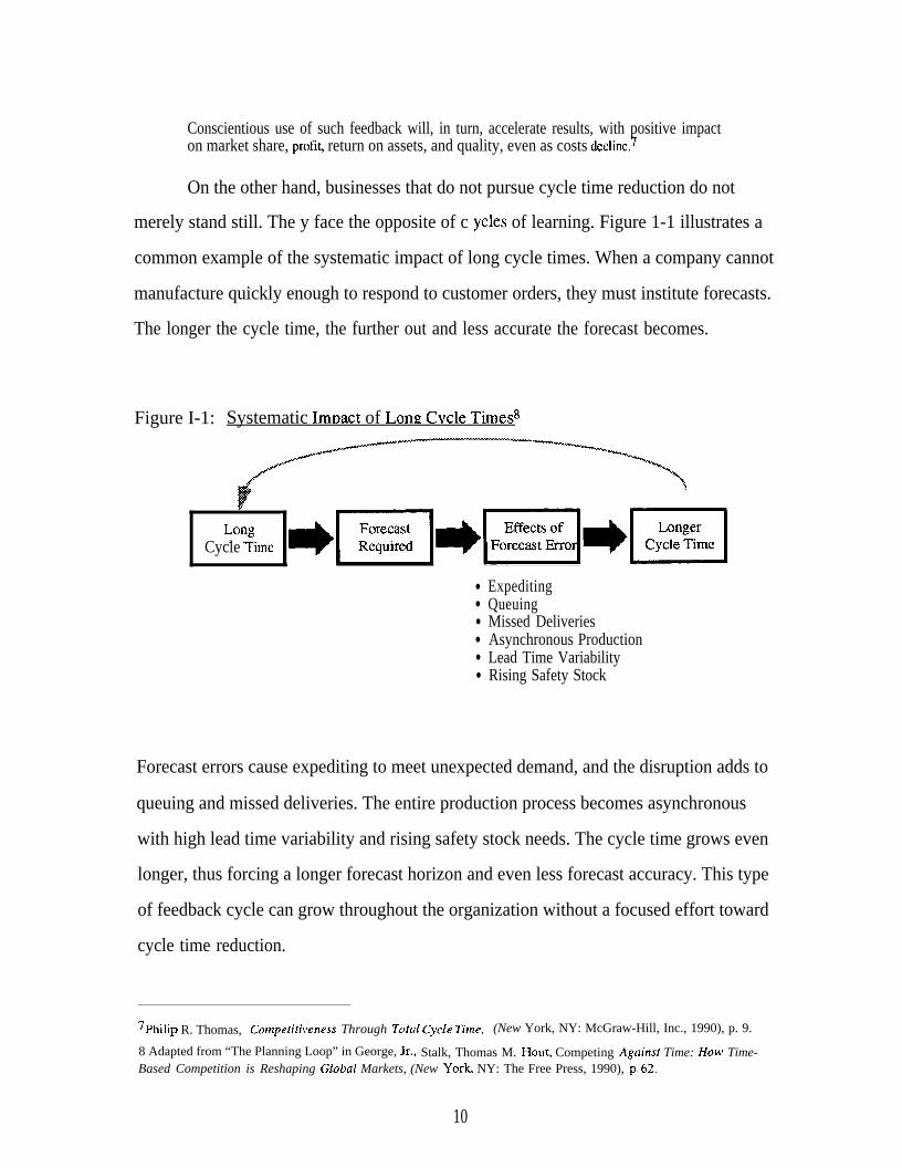
Conscientious use of such feedback will, in turn, accelerate results, with positive impacton market share, protit, return on assets, and quality, even as costs decline.7
On the other hand, businesses that do not pursue cycle time reduction do not
merely stand still. The y face the opposite of c ycles of learning. Figure 1-1 illustrates a
common example of the systematic impact of long cycle times. When a company cannot
manufacture quickly enough to respond to customer orders, they must institute forecasts.
The longer the cycle time, the further out and less accurate the forecast becomes.
Figure I-1: Systematic Impact of Lom.z Cycle Times8
‘on’,*ps+p=q*FlCycle Tune
●
●
●
●
●
●
ExpeditingQueuingMissed DeliveriesAsynchronous ProductionLead Time VariabilityRising Safety Stock
Forecast errors cause expediting to meet unexpected demand, and the disruption adds to
queuing and missed deliveries. The entire production process becomes asynchronous
with high lead time variability and rising safety stock needs. The cycle time grows even
longer, thus forcing a longer forecast horizon and even less forecast accuracy. This type
of feedback cycle can grow throughout the organization without a focused effort toward
cycle time reduction.
7Philip R. Thomas, Conlpetiti~*eness Through Total Cycle Time, (New York, NY: McGraw-Hill, Inc., 1990), p. 9.
8 Adapted from “The Planning Loop” in George, Jr., Stalk, Thomas M. Hout, Competing Against Time: How Time-Based Competition is Reshaping Global Markets, (New York NY: The Free Press, 1990), p. 62
10

1.1.2. Cycle Time Reduction at Kodak
Eastman Kodak Company has recognized these benefits of cycle time reduction
and has instituted programs throughout the organization in its efforts toward continuous
improvement. Top management launched a program in 1990 called K@ (Kodak Perfect
Process, Perfect Product) which calls for major improvement thrusts in 5 areas: cycle
time, invariance, cost, benchmarking, and new products.
A group of leaders for each area have responsibilities ranging from worldwide
sharing of successes to presenting an annual K@ quality conference. The vision of
Kodak management is revolutionary, not evolutionary improvement. Therefore, they
have mandated 25% improvement per year on key performance measures, which cannot
be attained without radically rethinking the business.
Despite these successes, the current pressure for improvement in the I@ areas is
stronger than ever. In 1991, Kodak’s long-term debt to equity ratio increased from 1.0 to
1.2 which included $600 MM in new borrowings.g Hence, the company’s debt structure
is constraining all capital expenditures and is highlighting the opportunity cost of funds
tied up in inventory. Cycle time and inventory reduction have become ingrained
concepts across the organization. The result is that this thesis is focused on some of the
most critical issues facing Kodak today,
‘9From the Eastman Kodak Company 1991 Annual Report:
~~~ng.Term B~rro~@~ ($MM) 7,597 6,989Shareowners’ Equity ($ MM) 6,104 6,748
Debt-to-Equity Ratio 1.2 1.0
11
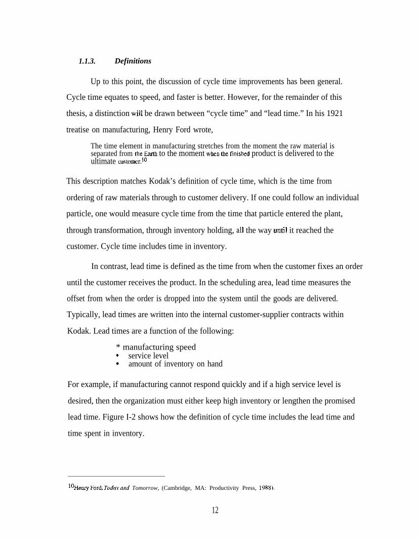
Up to this point, the discussion of cycle time improvements has been general.
1.1.3. Definitions
Cycle time equates to speed, and faster is better. However, for the remainder of this
thesis, a distinction will be drawn between “cycle time” and “lead time.” In his 1921
treatise on manufacturing, Henry Ford wrote,
The time element in manufacturing stretches from the moment the raw material isseparated from the &rth to the moment when the finMed product is delivered to theultimate customer.10
This description matches Kodak’s definition of cycle time, which is the time from
ordering of raw materials through to customer delivery. If one could follow an individual
particle, one would measure cycle time from the time that particle entered the plant,
through transformation, through inventory holding, all the way until it reached the
customer. Cycle time includes time in inventory.
In contrast, lead time is defined as the time from when the customer fixes an order
until the customer receives the product. In the scheduling area, lead time measures the
offset from when the order is dropped into the system until the goods are delivered.
Typically, lead times are written into the internal customer-supplier contracts within
Kodak. Lead times are a function of the following:
* manufacturing speed* service level● amount of inventory on hand
For example, if manufacturing cannot respond quickly and if a high service level is
desired, then the organization must either keep high inventory or lengthen the promised
lead time. Figure I-2 shows how the definition of cycle time includes the lead time and
time spent in inventory.
10Henry Ford TodaY and Tomorrow, (Cambridge, MA: Productivity Press, 1988).
12

Figure I-2: Definitions of Cycle Time and Lead Time
Cycle TimeI I
Lead Time Time in Inventory
Tl&fE ~
1.2. Industry Background
1.2.1. The Roll Coating Division
The Roll Coating Division (RCD) is located in the Kodak Park manufacturing site
in Rochester, NY. RCD produces film base (often called film support) which is
subsequently sensitized with photographic emulsion. The polyester film base (trade
name ESTAR) is used in rigid products such as microfiche, x-ray, and graphic arts films.
The RolI Coating ESTAR process has several key features :
● ESTAR production is a continuous process that runs 7 days per week,24 hours per day
● ESTAR machines are highly capital intensive● Several machines produce hundreds of items● Product changeovers create waste and the amount varies with sequence
These features mean that every minute not producing salable product is a minute of
revenue lost forever, valued at full opportunity cost. As early as 1921, Henry Ford
recognized the importance of this time dimension when he wrote,
Time waste differs from material waste in that there can be no salvage. The easiest of allwastes, and the hardest to correc~ is the waste of time, because wasted time does not litterthe floor like wasted material. In our industries, we think of time as human energy, If we

buy more material than we need for production, then we are storing human energy - andprobably depreciating its value.11
Each of the Roll Coating - ESTAR machines in Rochester are several stories tall,
a few hundred feet long, and several feet wide. Figure I-3 shows a schematic of a typical
machine. Hot polyester resin is extruded and cast on to a large coating wheel which
begins the cooling process. A web of material forms, which can then be heated and
stretched both lengthwise and widthwise (“drafting and teetering”). Finally, the web is
heat treated and wound in a roll several feet wide and several thousand feet long.
Production teams of operators and engineers are dedicated to each machine, and they staff
the equipment around the clock.
Figure I-3: Roll Coating ESTAR Process
PolyesterExtrusion
Casting
With hundreds of products to manufacture on only a few machines, setups
represent an critical part of ESTAR production. Setups can take anywhere from several
minutes to several hours. During that time, the machine must be running (and creating
waste) in order to bring up all the processes in control. Therefore, the setup cost includes
waste material as well as lost capacity and flexibility.
11 Henry Ford+ Today and Tomorrow, (Cambridge, MA: Productivity Press, 1988).
14

Sequencing is also critical in how long a setup takes. Width, thickness, color, and
coating features can all be changed, but products often share several of these
characteristics. Therefore, sequences of product that differ by only one characteristic at a
time can have faster setups than sequences of radically different products. Some products
may have features that only certain machines have the capability to manufacture.
Moreover, the high volume products may have weekly orders, while others may only
have one order each year (See Figure I-4). As a result, how to dedicate machines (if at
all) and how to schedule product sequences and lot sizes become a critical part of asset
utilization, inventory management, and the overall manufacturing strategy. These
decisions, in turn, affect the ESTAR department’s cycle time and impact the entire film
SUpply chain.
Figure I-4: Concentration of ESTAR Items
Estar Roll Coating Items
15
A planning department schedules the shop floor in response to the previously
discussed constraints:
●
●
●
●
●
●
●
●
Machine capabilityMachine capacityMachine speedProduct sequencing benefits
Customer orders and lead timesLot sizingInventory management
Scheduled machine maintenance
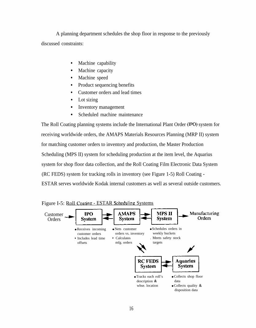
The Roll Coating planning systems include the International Plant Order (IPO) system for
receiving worldwide orders, the AMAPS Materials Resources Planning (MRP II) system
for matching customer orders to inventory and production, the Master Production
Scheduling (MPS II) system for scheduling production at the item level, the Aquarius
system for shop floor data collection, and the Roll Coating Film Electronic Data System
(RC FEDS) system for tracking rolls in inventory (see Figure 1-5) Roll Coating -
ESTAR serves worldwide Kodak internal customers as well as several outside customers.
Figure I-5: Roll Coatin z - ESTAR Schedulimz Systems
CustomerOrders -B==~m.””=yng
● Receives incoming ● Nets customer ● Schedules orders incustomer orders orders vs. inventory weekly buckets
c Includes lead time s Calculates . Meets safety stockoffsets mfg. orders targets
*H
E!14zEl● Tracks each roll’s ● Collects shop floor
description & datawhse. location ● Collects quality &
disposition data
16

1.2.2. The Film Manufacturing Supply Chain
The Roll Coating Division plays a vital role in the film manufacturing supply
chain. It transforms the raw chemicals into a roll of film base. Figure I-6 shows a
simplified version of the subsequent steps which include coating the film base with silver
halide emulsion (Sensitizing) and cutting and packaging the sensitized rolls (Finishing).
The structure of the supply chain includes 3 important characteristics:
●
●
●
Roll Coating and
An explosion of items as different coatings, sizes, and packages areintroduced downstream
An explosion of value as high cost materials and processes are addedA gradual decrease in lead time, especially in Finishing where multiplerelatively low cost pieces of.equipment are available and dedicated to aspecific business
Sensitizing are both highly capital intensive operations with one basic
manufacturing path, while Finishing less capital intensive with different “slit and chop”
paths and different packaging configurations.
Figure I-6: Sim lifi d V rsi n of he Film M nufact rin u 1 hain
~Fl
Increasing numbers of items ~
Increasing $ value
Decreasing lead times
From the days of its founder, George Eastman, Kodak has been a highly vertically
integrated company. That tradition remains apparent today as shown in Figure I-7 which

Figure I-7: The Sensitized Film Manufacturing Supply Chain
‘U’’tmu” ~Chemical
- D i s t i l l a t i o n —
414–––I‘l-—.I 1 \
~ Recovev _Polyester
b-+ Silver
Recovery
SyntheticChemicals
ISilver
Nitrating
KEY
~ Forward Material Flows
+– Recycled Material Flows
\
.—— — ———— ———— ————
4 4t !
.—— — ——— ——— ————I ?
I
I ~PolymerI
1 II-—— ——— ——— —- .—— — —I II
+--.-T. -J--3
I I III I I II-~ Roll Coating RoU
Chemical Coah”ng 1 1 11
~ Sensitizing ~bFinishing ‘—~ ~i~~u~!’n
I1
Film Emulsion~ Components
I i~ Manufacturing I Regional
Manl#acturing
L
1 I Distribution
7——— ——— ——— ——— ——— ——— —. I

expands the simple supply chain picture shown in Figure I-6. Many of the raw materials
for the film making process come from a Kodak-owned sector called Eastman Chemical
Company. As Figure I-7 illustrates, Kodak’s Imaging sector then transforms the raw
chemicals all the way to finished film packed in the familiar gold boxes and located in
regional warehouses. Often, this entire transformation process takes place at one site,
Kodak Park in Rochester, New York, where everything from the power to the packaging
is produced on location. Furthermore, as all the dashed arrows indicate, much of the
material flows in a closed recycle loop around the site.
Figure I-7 illustrates several key points:
● Eastman Chemical and Synthetic Chemicals12 (with some outsidepurchases) supply the raw materials
● Polyester polymer and chemicals supply Roll Coating ESTAR whichmakes film base (excluding the acetate process)
● Silver halide and other chemicals supply emulsion manufacturingwhich makes the sensitized film coating
“ Roll Coating’s film base and the emulsion supply Sensitizing whichcoats the film, creating what is called a “wide roll” of sensitized film
● Finishing then slits and chops the “wide roll” and packages it in goldboxes for distribution
The third case study in this thesis (Chapter IV, The Supply Chain Analysis) covers the
part of the of Figure I-7 that is in bold.
Another way to view the supply chain from a cycle time perspective is to use a
common tool at Kodak called an “Optim” diagram. Figure I-8 shows such a diagram for
the ESTAR supply chain. The horizontal axis represents the cycle time in days for an
item to be manufactured, stored in inventory, and transported to the next stage. The
vertical axis represents delivered unit cost or cumulative value added for each stage. The
area of each block shows the time-value of the stage and serves as a pareto chart of
improvement opportunity. The bigger the area, the bigger the potential savings.
12Four peviou~ Leadem For Manufac.ring intem~hlp~ t~~k place in tie s~thetic Chenlica]s Division in 1990 and
1991. See the theses of Christine N. Jutte, Bradley A. Koetje, Theresa Lai-Hing Mock, and Christopher P. Papouras.

Sometimes a very long cycle time item of low value such as “Syn Chem Inventory” can
be a lower priority (smaller area block) than a fast item of high value such as “Finishing”
(see Figure I-8). However, there may also be systematic effects embedded in the
diagram. For instance, the long Syn Chem c ycle times may create a need for longer
forecast horizons, which in turn may make the forecast less accurate and may force
downstream stages to hold extra inventory. The slanted lines on some of the boxes
represent the time and value of the actual transformation. A straight vertical line implies
that at a broad level of detail, the item can be treated as though it were bought at a point
in time and held in inventory.
Figure I-8: “()~tim” Diamnm of the Film Manufacturing Su~Pl~ C hain
1 Chemical Subbing Inv ‘ : Coatingpolymer : Inventory $d dInventory c 44z~
A
SilverNitrate M
Inv s Emulsionc~ Inventorymz
1Syn Chem Inventory
LE!ee=-
1 Gelatin Inventory H 1Cycle Time
WideRollInv
/
FinishedGoods
Inventory(including
DistributionCenters)
Note: Diagram box sizes are not to scale and do not represent the real data.
20

In short, this background on the Roll Coating business and on the film manufacturing
supply chain provides the context necessary for the three case studies in this thesis. The
description should help relate the case studies to each other and show why they represent
critical areas for Kodak and for manufacturing in general.
1.3. Thesis Overview
1.3.2. Problem Scope
This thesis addresses the key manufacturing issue of cycle time along with its
inventory component. The thesis makes a progression from detailed, limited scope
analysis all the way to high level, broad scope analysis. The problem addressed is always
“How can cycle time be reduced at this particular level?” The approach is always “How
can this work be implemented in a practical business situation’?”
The problem scope continually expands the definition of the system being
analyzed. It escalates from a single product all the way to an entire supply chain. The
approach involves three case studies:
“ The Single Product Analysis
“ The Single Machine Analysis
“ The Supply Chain Analysis
The thesis shows that as the scope of the analysis grows broader, the level of detail
diminishes. The conclusion will be that the approach, the analytic tools, and the solution
must be tailored to the breadth of the problem. Therefore, the definition and scope of
each case study is critical.

1.3.3. Problem Approach
The Single Product Analysis addresses the trade-off between lot size and
inventory level for just one product at a time. Because it is limited to a single product,
the analysis can include the effects of demand variability and lead time variability. It can
account for the volume sold while the machine is in the process of manufacturing the
product. Moreover, its simplicity allows it to model many products and many sensitivity
scenarios very quickly and easily. Thus, it can be used to build process intuition about
the effect and sensitivity of various parameters such as setup time, supply variability, and
service level. P&o, it can be used to prioritize improvement efforts for every ESTAR
product.
The Single Machine Analysis addresses a broader problem. By looking at a
collection of products that run on one machine, it can incorporate the impact of capacity
constraints and setup sequencing efficiencies. It does not include the detailed variability
issues of the Single Product Analysis; but it can take the perspective of a whole machine.
The Single Machine Analysis can create an optimum schedule of products, both
sequence and lot size, over multiple periods for an ESTAR machine.
The Supply Chain Analysis addresses how product and machine decisions in one
department can affect the upstream suppliers and downstream customers. It determines
how inventory can be strategically re-positioned across the supply chain to minimize
cycle time and cost for the company as a whole. The scope of the Supply Chain Analysis
extends well beyond the Roll Coating Division to include both the Sensitizing and the
Finishing operations. It does not provide the detail of the previous two case studies, but it
does provide the most comprehensive look at the cycle time and inventory issue. As a
result, the Supply Chain Analysis provides the most leverage and the most cost savings of
the three case studies.
22

1.3.4. Conclusions
The estimated value of the three case studies is over $7 million in annual cost
savings (see Figure 1-9). The first column shows the savings that have firm
implementation plans due by the end of 1993 or earlier. 13 The second column of “case
study savings” shows just the savings shown by representative case studies that were
actually modeled. The third column shows the effect of roiling out those case studies
across all ESTAR products. Note that the Supply Chain Analysis shows negative $0,5
million in this column. That figure represents an investment in inventory that would
Figure 1-9: Potential Annual Savings from the Thesis Projects
Terms are $MM
PROJECT
● Single Product Analysis– Lot Sizing& Inventory
* Single Machine Analysis– Capacity& Sequencing
● Supply C~ain Analysis– Strategic Inventory
Placement
Totals
ImplementedSavings in ’93(Supply Chain)
0.5
0.0
0.1
Case Study-
(Supply Chain)
1.3
0.1
0.8
Total Potential Total PotentialSalduis
(Estar Dept only)
2.5
0.4
(0.5)
Swi!uEi@star supply
Chain)
2.5
0.4
4.4
c10.6 2.2
Note: Inventory Reductions are evaluated at 35% annual savings
2A •17.3
13~e 1993 fiPlemented ~av~~~ for he Sin@e pr~du~t Analysis were pledged independency of this work, but include
waste and inventory savings addressed by the model. The 1993 implemented savings for the Supply Chain Analysisrepresent a pilot program that directly resulted from this thesis work.
23

result in a net cost reduction if the whole supply chain were considered. That is precisely
what the last column does. It shows that the $7 million savings potential comes from
implementing all three case study analyses throughout the Rochester ESTAR department
and its associated supply chains. It represents a stretch goal and indicates the order of
magnitude of this thesis work on bottom-line cost savings,
The conclusion of this thesis is that the nature of the problem dictates the
appropriate level of detail, but there is tremendous value in looking across the entire
supply chain. Cycle time reduction represents a key corporate strategy that affects not
just each department, but also all of the interconnections. For some organizations, this
becomes the most important theme in the business:
The overriding goal [at Toyota] is to never [sic] inconveniencedownstream customers.14
The vision involves becoming a “supply chain leader.” 15 As the supply chain cycle time
is further and further compressed, the utmost limit becomes zero inventory between
stages. At this point, the stages are coupled and lead time and capacity are synchronized.
The supply chain has reached its ultimate cycle time goal of being directly tied to the
customer.
14Masaaki Imai, WZEN: l%e Key to Japan’s Competitive Success, (New York, NY: Random House BusinessDivision, 1986), p. 135.15 George, Jr., Stalk, Thomas M. HOUL Competing Against Time: How Tin~e-Based Competition is Reshaping GlobalMarkets, (New York, NY: The Free Press, 1990), p. 237.
24
Chauter II. Single Product Analvsis
Because the Roll Coating - ESTAR department has few machines that produce
almost 200 distinct items, frequent product changeovers and setups are necessa~.
Therefore, lot sizing and inventory trade-off issues become critical both on the shop floor
and in the planning arena. The Single Product Analysis addresses this cross-functional
trade-off with a data driven model. The model suggests that Roll Coating - ESTAR could
save up to $2 MM annually at current capability by adjusting operating policies on all
their products. Moreover, they could save an additional $0.5 MM annually if they could
also reduce setup times by 50%.
The reason for introducing the model is that the ESTAR department determines
lot sizes without considering inventory costs. The product engineers calculate the
average setup waste for a product, and from that, the average setup cost. Then they
balance the setup cost with the product’s profit per foot (net of the running waste). once
enough salable feet are produced for the profit to equal the waste, the product reaches
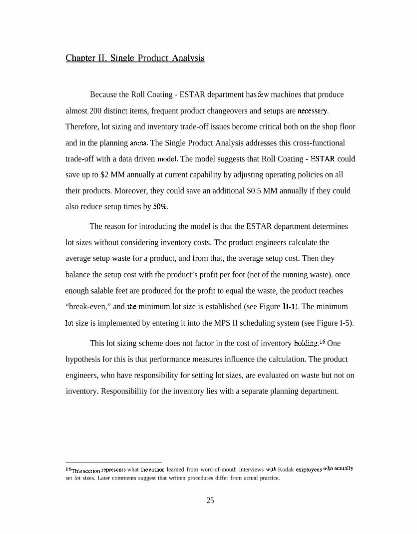
“break-even,” and the minimum lot size is established (see Figure 11-1), The minimum
lot size is implemented by entering it into the MPS II scheduling system (see Figure I-5).
This lot sizing scheme does not factor in the cost of inventory holding.lb One
hypothesis for this is that performance measures influence the calculation. The product
engineers, who have responsibility for setting lot sizes, are evaluated on waste but not on
inventory. Responsibility for the inventory lies with a separate planning department.
16~i~ ~ectlon ~epre~ent~ what tie au~or learned from word-of-mouth interviews ~if.h Kodak emPl~Yees wbo ac~allY
set lot sizes. Later comments suggest that written procedures differ from actual practice.
25

Figure II-1: Lot Sizing Method
Lot Size Chosen Such That:
GoodProduct
Waste
[
Lot % 1 [ Lot %U@l= $ Setup +
Size ● Good ● FootK!2Sl
Waste Size ● Running ● ~wt(Feet) Product (Feet) waste 1
11.1. Goals
The ultimate goal for the Single Product Analysis is to create a simple model
reflecting the macro-drivers of the business. Related to the discussion above, one clear
purpose of the model is to incorporate inventory costs into the lot sizing strategy.
Other objectives of the Single Product Analysis include:
● Providing concrete, irnplementation-ofiented outputs● Prioritizing lot size and setup reduction opportunities for the top few
ESTAR products that constitute most of the annual volume“ Quantifying sensitivity to setup time, supply variability, and service
level● Providing process intuition for both the engineers and the planners
The Single Product Analysis focuses on setup time reduction because it is the key
to unlocking Roll Coating - ESTAR’S production constraints. The model translates faster
setups into decreased lot sizes and increased run frequencies by providing specific
26
numerical outputs. 17 If one product retains a long setup time, then the economics
mandate long, infrequent runs. This constraint will in turn affect the other products
which must run on the same machine. They must wait for the long-running product, and
as a result, they become more difficult to schedule and require more safety stock. In
contrast, fast setup products can justify frequent changeovers with short runs, and this
capability frees the machines to respond quickly to swings in demand or production
problems. The final result is improved customer response and service which can provide
a distinct advantage in the competitive film market.
11.2. Methodology
The methodology behind the Single Product Analysis is a lot size, reorder point
system. 18 This type of system utilizes specific process data to generate detailed results
for one product at a time. This methodology has a fundamental trade-off. Although the
outputs are specific and operational, they may not be optimal or even feasible when all
the products in the department are looked at together.
17 The single product analysis does not specify how to reduce setup times. It values and prioritizes setup timeimprovements and specifies how to cash out the benefits. In Estar Roll Coating, methods to reduce setup times include:
● Organizational emphasis, measurement, and rewards focused on the issue“ Choreographing setups in advance using an experienced team“ Performing some tasks off-line before the changeover● Moving tasks from series to parallel
An excellent general resource on setup time improvement is: Shigeo Shingo, A Revolution inManufacturing: the WED Syslem, (Cambridge, MA: Productivity Press, 1985)
The general strategy behind Single Minute Exchange of Dies involves 4 stages:o.
1.2.3.
Dissecting the set~p in detail using vfieotape to identify every step and whether it is “internal”or “external”Ensure that only “internal” steps are performed when the machine is downConvert “internal” steps to “external” ones by breaking old habitsStreamline, standardize, simplify every “internal” step remaining
– One-mm screws– Visible, calibrated settings– Special jigs and part holders
18~1~ is sometfies called ~ iterative (Q,R) ~ocedue, see for inst~ce Thomas E. Vollmann, William L. Berry, ~d
D. Clay Whybark, Manwfactun”ng Planning and Control Syste/nst (3rd ed. Homewood+ ~: Business me ~in~1992), pp. 728–729.
27
There are several key features in the Single Product Analysis that take it beyond
simple Economic Order Quantity calculation 19 including:
● Input of supply variability in the form of a mean lead time and itsstandard deviation (i.e.. a lead time of 2 weeks t 1 week)20
a
● Input of demand variability in the form of a mean demand per time andits standard deviation (i.e.. a demand of 1,000 feet per week* 200 feetper week)
● Calculation using finite production time to manufacture an order(versus instantaneous arrival as if purchasing from the outside)
c Calculation of an imputed stockout cost to quantify the costs andbenefits of selecting a particular customer service level
In specific detail, Table II-1 lists the model inputs and outputs. The appendix
(section VI. 1) elaborates on the calculations used and shows sample model outputs.
Although this methodology represents a general approach applicable to a wide
variety of situations, there are two features unique to Kodak and film manufacturing:
● Discrete run frequency possibilities
● Correlation of waste to the entire lot
Discrete run frequency possibilities mean that there are only a finite number of choices
(weekly, hi-weekly, monthly, etc.) for how often Kodak can run a batch. This is because
in Roll Coating - ESTAR and in Sensitizing operations, there is capital intensive, capacity
constrained equipment that causes scheduling competition for resources. Using only a
finite number of frequencies provides scheduling convenience and allows coordination
with other parts of the production process. The implications are that 1) run frequent y
analyses do not need to be precise to the day, and 2) this paradigm may need to be
challenged as manufacturing processes become more flexible. Correlation of waste to the
1913fiple Economic ~der Qu~ntit~ ~n~lySIS ~SSUmeS tie order ~ives instant~eously and that there is neither SUpply
nor demand variability. If this the case, one can set the inventory holding cost equal to the setup cost and solve directlyfor the quantity without using any calculus. See for instance Barry Renden and Ralph M. Stair, Jr., QualitativeAnalysis for Management., 4th cd., (Boston, MA: Allyn and Bacon, 1991).
20As defined in section I-l .3., this lead time represents how long it t~es to get tie prodLlct on the machine including
raw material procurement and competition for resources by other products. The lead time here is nor the “touch time.”
28
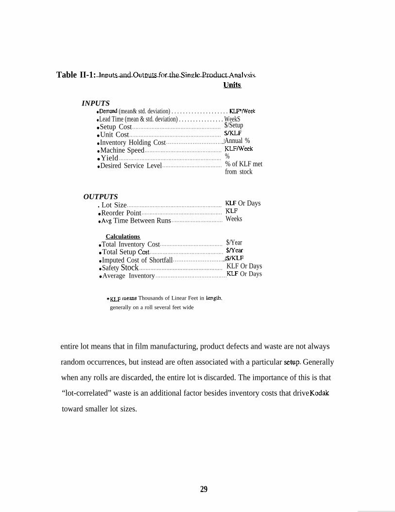
Table II-1: Inmts and Out~uts for the Simzle Product AnalvsisUnits
INPUTS● Demand (mean& std. deviation) . . . . . . . . . . . . . . . . . . . . KLF*/Week● Lead Time (mean & std. deviation) . . . . . . . . . . . . . . . . WeekS● Setup Cost . . . . . . . . . . . . . . . . . . . . . . . . . . . . . . . . . . . . . . . . . . . . . . . . . . . . . . . $/Setup● Unit Cost . . . . . . . . . . . . . . . . . . . . . . . . . . . . . . . . . . . . . . . . . . . . . . . . . . . . . . . . . $/KLF● Inventory Holding Cost . . . . . . . . . . . . . . . . . . . . . . . . . . . . . . . ...!Annual %● Machine Speed . . . . . . . . . . . . . . . . . . . . . . . . . . . . . . . . . . . . . . . . . . . . . . . . KLF/Week● Yield . . . . . . . . . . . . . . . . . . . . . . . . . . . . . . . . . . . . . . . . . . . . . . . . . . . . . . . . . . . . . . . . %● Desired Service Level . . . . . . . . . . . . . . . . . . . . . . . . . . . . . . . . . . . . . % of KLF met
from stock
OUTPUTS. Lot Size . . . . . . . . . . . . . . . . . . . . . . . . . . . . . . . . . . . . . . . . . . . . . . . . . . . . . . . . . . . KLF Or Days● Reorder Point . . . . . . . . . . . . . . . . . . . . . . . . . . . . . . . . . . . . . . . . . . . . . . . . . . KLF● Avg Time Between Runs . . . . . . . . . . . . . . . . . . . . . . . . . . . . . . . . Weeks
Calculations● Total Inventory Cost . . . . . . . . . . . . . . . . . . . . . . . . . . . . . . . . . . . . . . . $/Year● Total Setup Cost . . . . . . . . . . . . . . . . . . . . . . . . . . . . . . . . . . . . . . . . . . . . . . $Near● Imputed Cost of Shortfall . . . . . . . . . . . . . . . . . . . . . . . . . . . . ...4$/KLF● Safety Stock . . . . . . . . . . . . . . . . . . . . . . . . . . . . . . . . . . . . . . . . . . . . . . . . . . . . KLF Or Days● Average Inventory . . . . . . . . . . . . . . . . . . . . . . . . . . . . . . . . . . . . . . . . . .KLF Or Days
*KJF mems Thousands of Linear Feet in leng~,
generally on a roll several feet wide
entire lot means that in film manufacturing, product defects and waste are not always
random occurrences, but instead are often associated with a particular setup. Generally
when any rolls are discarded, the entire lot is discarded. The importance of this is that
“lot-correlated” waste is an additional factor besides inventory costs that drive Kod&
toward smaller lot sizes.
29
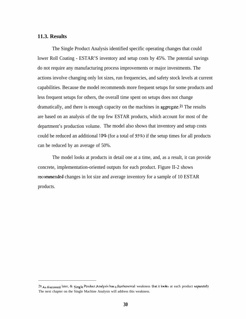
11.3. Results
The Single Product Analysis identified specific operating changes that could
lower Roll Coating - ESTAR’S inventory and setup costs by 45%. The potential savings
do not require any manufacturing process improvements or major investments. The
actions involve changing only lot sizes, run frequencies, and safety stock levels at current
capabilities. Because the model recommends more frequent setups for some products and
less frequent setups for others, the overall time spent on setups does not change
dramatically, and there is enough capacity on the machines in aggregate.21 The results
are based on an analysis of the top few ESTAR products, which account for most of the
department’s production volume. The model also shows that inventory and setup costs
could be reduced an additional 10~0 (for a total of 5570) if the setup times for all products
can be reduced by an average of 50%.
The model looks at products in detail one at a time, and, as a result, it can provide
concrete, implementation-oriented outputs for each product. Figure II-2 shows
~ecommended changes in lot size and average inventory for a sample of 10 ESTAR
products.
21 AS di~cu~~ed later, & Single product Anal~~i~ has a fundanlental weakness that it looks at each product separately.
The next chapter on the Single Machine Analysis will address this weakness.
30

Figure II-2: St)ecific ODerational Recommendations of the Sinde Product Analysis22
200%
150%
g 10096ae
50%3gak o%&
-50%
-100% I I I I a I I I [
I I9 aJ B
1’2 ~ 4 5 6 7 8 9 101 I n I
Sample Produc@
Figure II-3 shows the bottom line dollar value of making the recommended
operating changes. Notice that for products 2 – 5, when the lot sizes are reduced, the
corresponding setup costs are increased. The result of this small investment in smaller
lots and more frequent runs is a dramatic reduction in inventory holding costs. The
model’s capability to offset small setup waste increases with large inventory cost
decreases in the face of supply and demand variability is critical for the Roll Coating
Organization. The simultaneous trade-off of waste and inventory challenges a paradigm
of keeping the two issues separate at Kodak. The model results force a re-thinting of the
current organization where production is responsible for waste and a separate plzmning
department is responsible for inventory.
22The reason that lot size can increase while inventory simultaneoLlsly decreases (products 1,6,7,8,9, and 10) IS thatthese changes represent differences from current actual jgures>
That is, if the lot sizes stayed the same as they are
currently (or decreased), the inventory reductions would be even grearer than those shown in Figure II-2.
31
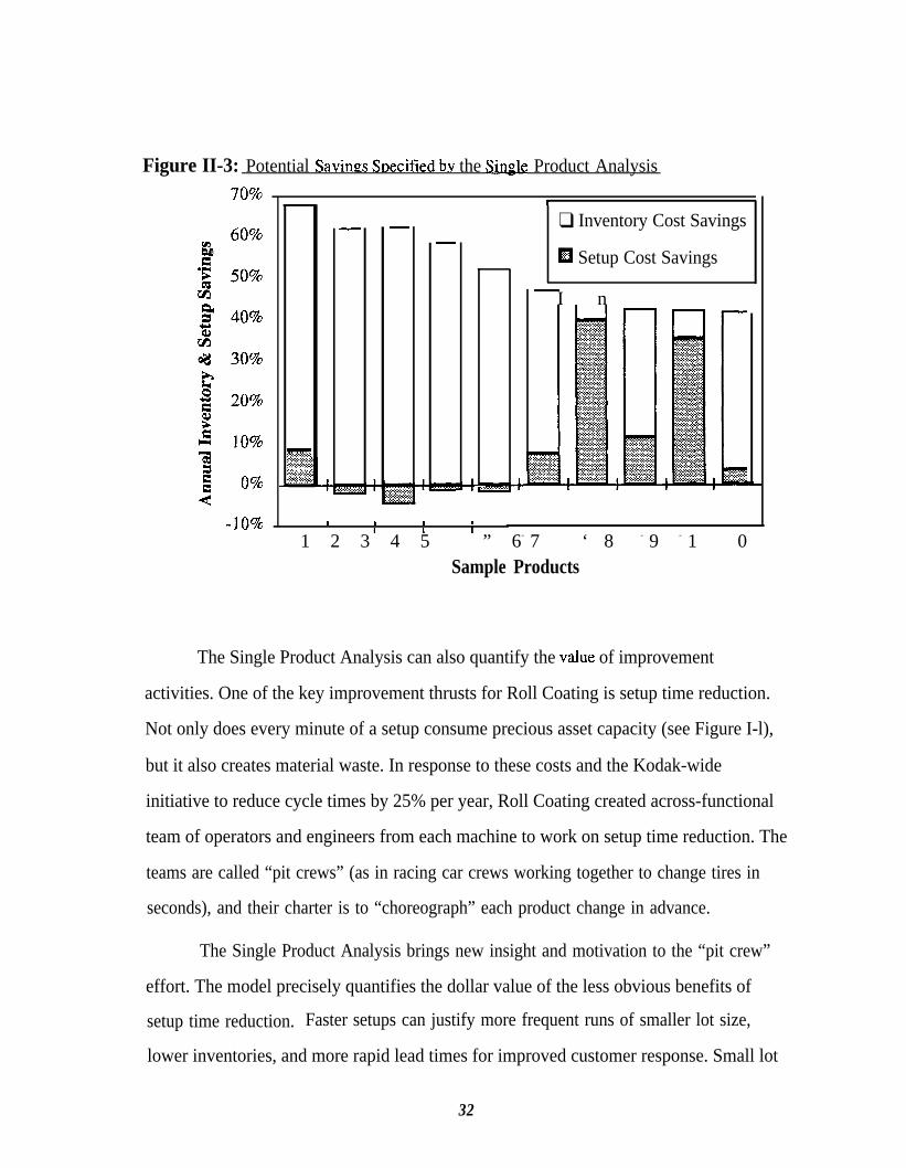
Figure II-3: Potential Savinm SDecified bv the Single Product Analysis
+ + +
t
.. ... ... . . .. . . . ... ....%......-.%..y.=-.:.:-:....:.::y.:::.:.~d
i II
II
II
1 2 3 4 5 ” 6- 7 ‘ 8 - 9 - 1 0
+
❑ Inventory Cost Savings
El Setup Cost Savings
I n
Sample Products
The Single Product Analysis can also quantify the vahe of improvement
activities. One of the key improvement thrusts for Roll Coating is setup time reduction.
Not only does every minute of a setup consume precious asset capacity (see Figure I-l),
but it also creates material waste. In response to these costs and the Kodak-wide
initiative to reduce cycle times by 25% per year, Roll Coating created across-functional
team of operators and engineers from each machine to work on setup time reduction. The
teams are called “pit crews” (as in racing car crews working together to change tires in
seconds), and their charter is to “choreograph” each product change in advance.
The Single Product Analysis brings new insight and motivation to the “pit crew”
effort. The model precisely quantifies the dollar value of the less obvious benefits of
setup time reduction. Faster setups can justify more frequent runs of smaller lot size,
lower inventories, and more rapid lead times for improved customer response. Small lot
32
sizes can be extremely important because defects tend to be associated with an entire run
of one product. As previously mentioned, when rolls need to be re-worked or discarded,
usually the entire lot “is involved, so smaller lots can help reduce that cost.
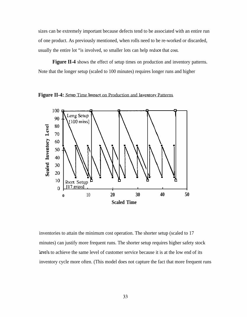
Figure II-4 shows the effect of setup times on production and inventory patterns.
Note that the longer setup (scaled to 100 minutes) requires longer runs and higher
Figure II-4: Setu~ Time Inmact on Production and Inventorv Patterns
Short Setup 1
I
I I
[17 minsr , uI I I
o 10 20 30 40 50Scaled Time
inventories to attain the minimum cost operation. The shorter setup (scaled to 17
minutes) can justify more frequent runs. The shorter setup requires higher safety stock
levels to achieve the same level of customer service because it is at the low end of its
inventory cycle more often. (This model does not capture the fact that more frequent runs
33

have a shorter planning horizon, and thus less demand variability. This effect can be
large enough actually to have lower safety stock with more frequent small batches.z3)
Figure II-5 shows the sensitivities of cost, lot size, and average inventory to the
spectrum of setup times. Because the relationships are not linear, the model proves very
useful in setting specific lot size quantities and cost targets for each product. Moreover,
the model demonstrates the real dollar values of waste and inventory for each setup
improvement, which can provide new process intuition.
Figure II-5: Sensitivity to Setup Time
100
90
80
70
60
50
40
30
20
10
0
1~ Optimum Lot Size/
o 20 40 60Scaled Setup Time
80 100
~uday s. Km~&~~ ~~d Milind M. Lde, “The Marketing/ Manufacturing Interface: Strategic Is sues.” University of
Rochester Center for Manufacturing & Operations Management Working Paper Series, CMOM 89-10, 1991, p. 13.
34

The Single Product Analysis can quantify operational sensitivity to many other
parameters besides setup time. These parameters include service level, demand
variability, lead time variability, and inventory holding cost. For example, Figure II-6
shows how different service level targets affect production and inventory patterns.
Service level here is defined as the percentage of demand in linear feet met from stock.24
Note that higher service requires just slightly more frequent runs and higher safety stock.
In the case of Roll Coating - ESTAR, service levels below 90% tend to require zero
safety stock under normal operating conditions.
Figure H-6:~Patterns
140
120
0
. .
. .
Lo
o
I
1
ervice ‘99%]
~i
lervice85%1 ; ,
10 20
\
[
\
\
\I1 4
30Scaled Time
40 50
24see “Type 2 Service “ in Steven Nahrnias, Production and Operations Analysis, &Iomewood, IL: Richard D. Irwin,hlC., 1989), p. 202.
35

Figure II-7 shows the sensitivity of the model outputs to different service levels.
As higher service levels are desired, at current manufacturing capability, the total cost
rises much faster than linearly. This cost and the expected number of stockouts at a given
service level can be used to calculate the cost per stockout to a customer. The model
outputs include this imputed stockout cost, and it can help in setting service levels that
optimize the trade-off between responsiveness and cost. Basically, the model can provide
a quantitative answer to the question, “What does it cost to provide a service level of X?”
This cost can then be balanced against what the customer is willing to pay to receive that
service level.
Figure II-7: ~ensitivitv to Service Level
1--
50-O*.0-
.* ---0------- ----- .----”
40 Avg Inventory30
20
10t
100
90
80
70
60
—— --~
Setup + Inventory Costs--
0 I 1I
I1 1
85% 90% 95% 10070
Desired Service Level
36

The Single Product Analysis can provide detailed, operational outputs in response
to different improvement efforts and planning decisions. It can quantify and prioritize
actions based on their contribution to the bottom line. It can even provide process
understanding and intuition about inter-relationships among different operating
parameters.
The Single Product Analysis, however, has one serious limitation: it can examine
only one product at a time. The key to controlling lead time variability and the resulting
queues and missed due dates is the proper choice of lot sizes. Furthermore, queuing is a
joint effect of multiple items competing for h.rnited resources.25 The whole system of
products, not one single product, determines the lead time variability. The model outputs
for lot size and run frequency for each ESTAR product calculated individually maybe
impossible to schedule when combined due to machine capacity and capability issues.
The facility is a 24-hour, 7-day operation running at high utilization. Certain products
can only be run on certain machines. Z7ze lot size and run &equency of one product
cannot be determined in a vacuum.
The analogy of traffic driving through an intersection works well here. Unless
volume is very small, a four-way stop, which takes each car (or product) separately, will
create large queues. A traffic light should meter flow according to overaIl load.
Accounting for all the waiting cars as a whole, the light should have short cycles (small
batches) when lightly loaded and long cycles (large batches) when heavily loaded. It is
not an individual car (or product) that determines the travel time, but rather the whole
flow of traffic.
All this is not to say that the Single Product Analysis cannot be useful. The
following section on implementation shows how it can be utilized in a practical fashion.
25This line of reasoning is based on Eliyahu M. Goldratti The Haystack Syndrome: Si~ing Information Out of the DataOcean, (Croton on Hudson, NY: North River Press, 1990).
37

However, this shortcoming, and indeed the theme of this thesis, points out the value of
expanding the problem treatment to a more global basis. The next section, which covers
the Single Machine Analysis, addresses the fundamental limitation of examining just one
product. There is a cost, though. As the scope of the analysis grows, the level of detail
diminishes. The Single Product Analysis provides the most comprehensive output of any
effort in the thesis.
11.4. Implementation
The Single Product Analysis is in the process of being implemented in Roll
Coating - ESTAR. While it is being used to help with the annual planning cycle and with
developing process intuition, its main use is in driving setup time reductions. The benefits
of setup time improvement activities can be analyzed and prioritized using outputs from
the Single Product Analysis. In particular, the top few Roll Coating - ESTAR products
were put in a pareto chart ranked on the benefit of reducing setup time by 50910. The “pit
crew” teams could then prioritize their setup time efforts and select the one or two highest
value opportunities for their machine with a definite financial target. The model
determines the overall value of setup time improvements by blending factors such as
annual volume, material cost, cument setup time, and yield. Note that the pareto chart in
Figure II-8 also shows the combination of waste and inventory savings that minimize
overall cost. Making both the waste and inventory targets visible is important because
the production department has an incentive to reduce only waste. At the extreme, setup
time reductions could be used solely to lower waste if run frequencies and inventories
remained constant. While this strategy would make the production department’s
measures look the best, it would not minimize cost for the company.
38
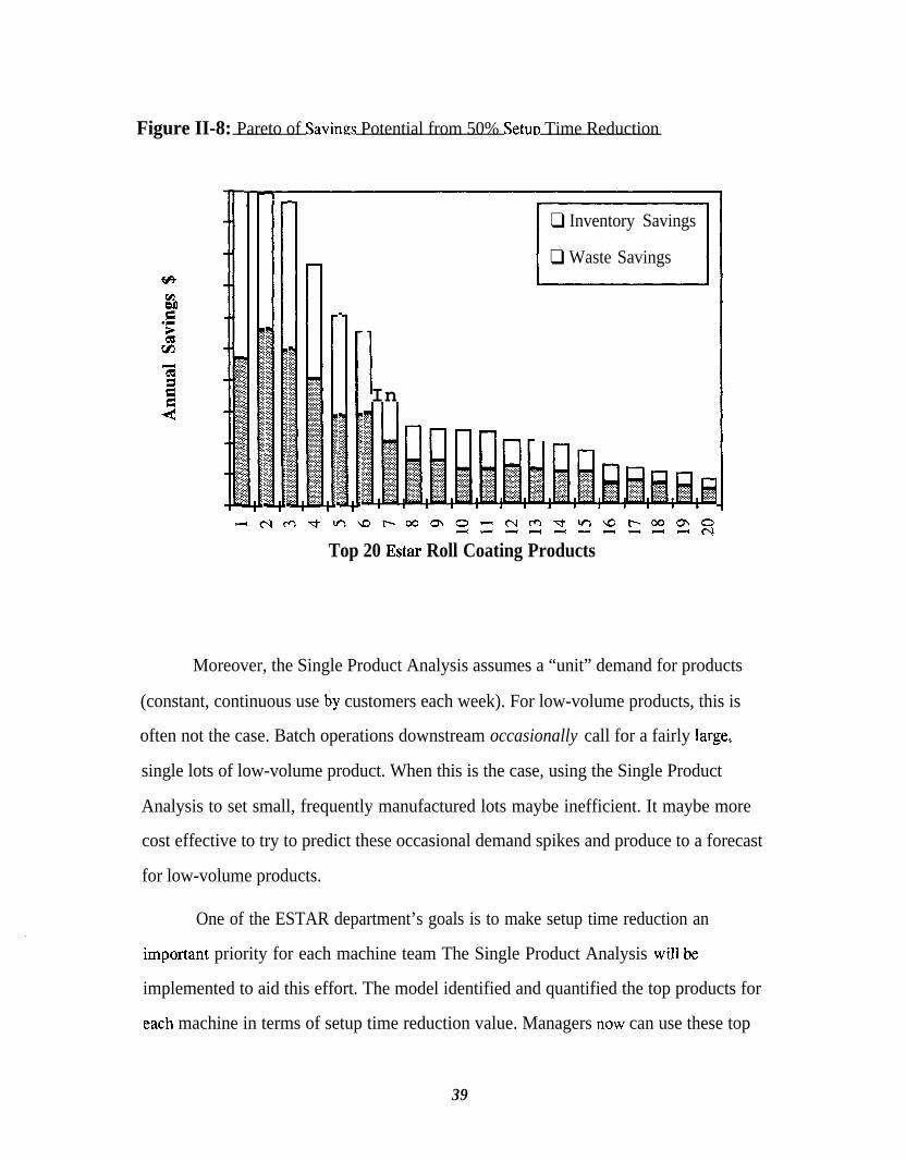
Figure II-8: Pareto of Savinzs Potential from 50% SetuD Time Reduction
❑ Inventory Savings
❑ Waste Savings
In+11:.:.:... . .
Top 20 Estar Roll Coating Products
Moreover, the Single Product Analysis assumes a “unit” demand for products
(constant, continuous use by customers each week). For low-volume products, this is
often not the case. Batch operations downstream occasionally call for a fairly large,
single lots of low-volume product. When this is the case, using the Single Product
Analysis to set small, frequently manufactured lots maybe inefficient. It maybe more
cost effective to try to predict these occasional demand spikes and produce to a forecast
for low-volume products.
One of the ESTAR department’s goals is to make setup time reduction an
“mportant priority for each machine team The Single Product Analysis will be
implemented to aid this effort. The model identified and quantified the top products for
each machine in terms of setup time reduction value. Managers now can use these top
39
product opportunities to set numerical goals for each machine team’s performance matrix.
The performance matrix, in turn, is used in employee evaluations that determine
promotions and compensation. In this way, the engineers and operators associated with
each machine will know that their priorities are aligned with the corporate vision for
cycle time reduction.
The most important result from the Single Product Analysis is the expansion of
Roll Coating’s lot size thinking to include inventoly considerations. Further opportunities
to reduce setup times, optimize lot sizing, and change limited performance measures will “
always exist. The single product model represents the first step in this direction.
40

Chat)ter III. Single Machine Analvsis
Because the lot size and run frequency for one product cannot be determined
vacuum (see section 11.3), the scope of the Single Product Analysis was increased to
include the dynamics of an entire ESTAR machine at once. The Single Machine
in a
Analysis covers all the products that are run on one machine for a given period of time.
Given the order due dates, setup times, and the capacity constraints, the Single Machine
Analysis produces the minimum cost, feasible schedule.2b On one ESTAR machine
alone, the model determined a schedule that could save thousands of dollars per year.
111.1. Goals
The goal of the Single Machine Analysis is to expand the scope of the product
analysis and make the results more implementable across the ESTAR department.
Specifically, by looking at the problem at a machine level, the analysis can include:
“ Sequencing effects on setup times● Capacity limits
The sequencing effects arise because the time required to setup a given product is
not fixed.z~ It depends on which product precedes it. As previously mentioned, this is
because each product has a number of parameters such as width, thickness, color, and
coating features which might or might not be the same as the preceding product.
Changing shades of blue may take on the order of minutes while changing thickness can
26The current literature often refers to “the single machine case,” but it differs greatly from the Single MachineAnalysis. The literature does not account for sequencing; it assumes product sequence does not affect setup time,which is not the case in Estar Roll Coating. In addition, the literature does not minimize cost, but tends to minimizeaverage time in the system, average number of jobs in the system, WIP, or average job lateness. The standarda~gonthm is “shortest processing Time” (SP’T) which means do the shortest job f~st and the longest job last. SeeThomas E. Vollmann, William L. Berry, and D. Clay Whybark, Manujactuting Planning and Control Sysrems, (3rded. HomewooL IL: Business One Irwin, 1992), pp. 535-536.27The single product analysis uses a freed setup time based on the most common sequence of products.
41

take substantially longer. Cument practice in Roll Coating is to follow
products on each machine that smoothes the changeovers and prevents
extreme, back-and-forth patterns. This fairly rigid sequence, however,
a sequence of
the setups from
does not vary with
loading. When utilization is low, Roll Coating might be missing an opportunity to reduce
inventory or reduce lead times by changing the setup sequence. The Single Machine
Analysis optimizes the sequencing relative to the load. When capacity is full, the
minimum time sequence is used. When capacity is not full, the minimum overall cost
sequence is used. This variable sequencing challenges the cument paradigm in Roll
Coating where breaking the standard order of products is considered an extraordinary
event that hurts the waste performance measure.
The Single Machine Analysis also improves on the Single Product Analysis by
including a capacity constraint. The model can limit the hours per week of setup and
production time.
111.2. Methodology
The Single Machine Analysis addresses the basic problem of how Roll Coating -
ESTAR should schedule one machine to minimize the cost of meeting demand. The
analysis models the simplest machine in the department. The analysis covers four weekly
buckets of demand and assumes no backordering is allowed (100% service level). Table
III-1 lists the required data inputs and model outputs.
42
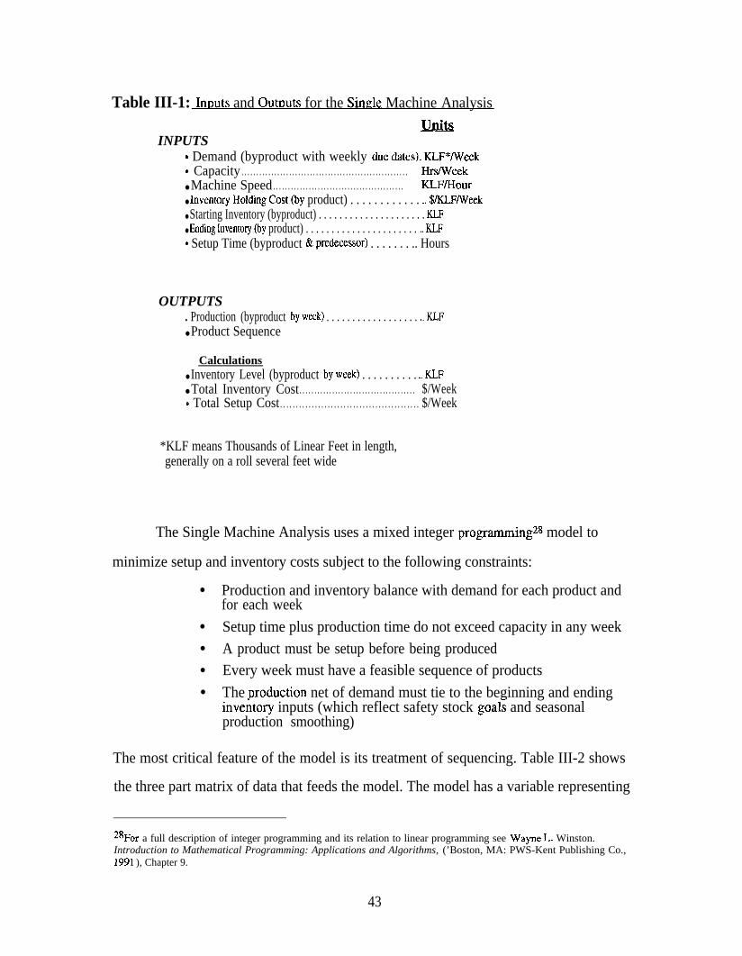
Table III-1: Intmts and Outt)uts for the Sin~le Machine Analysis
unitsINPUTS
“ Demand (byproduct with weekly duedates). KLF*/Week“ Capacity . . . . . . . . . . . . . . . . . . . . . . . . . . . . . . . . . . . . . . . . . . . . . . . . . . . . . . . . Hrs/Week● Machine Speed . . . . . . . . . . . . . . . . . . . . . . . . . . . . . . . . . . . . . . . . . . . . KLF/Hour● Invento~Holding Cost(by product) . . . . . . . . . . . . ..$~F~eek● Starting Inventory (byproduct) . . . . . . . . . . . . . . . . . . . . . K.LF● Ending Invento~(by product) . . . . . . . . . . . . . . . . . . . . . . ..~Fo Setup Time (byproduct &predecessor) . . . . . . . .. Hours
OUTPUTS. Production (byproduct byweek) . . . . . . . . . . . . . . . . . . ..KLF● Product Sequence
Calculations● Inventory Level (byproduct byweek) . . . . . . . . . . ..KLF● Total Inventory Cost . . . . . . . . . . . . . . . . . . . . . . . . . . . . . . . . . . . . . . . $/Weeko Total Setup Cost . . . . . . . . . . . . . . . . . . . . . . . . . . . . . . . . . . . . . . . . . . . . $/Week
*KLF means Thousands of Linear Feet in length,generally on a roll several feet wide
The Single Machine Analysis uses a mixed integer programmingzs model to
minimize setup and inventory costs subject to the following constraints:
●
●
●
●
●
Production and inventory balance with demand for each product andfor each week
Setup time plus production time do not exceed capacity in any week
A product must be setup before being producedEvery week must have a feasible sequence of products
The t)roduction net of demand must tie to the beginning and endinginvefitory inputs (which reflect safety stock goal: and seasonalproduction smoothing)
The most critical feature of the model is its treatment of sequencing. Table III-2 shows
the three part matrix of data that feeds the model. The model has a variable representing
28For a full description of integer programming and its relation to linear programming see Wa~e L. Winston.Introduction to Mathematical Programming: Applications and Algorithms, (’Boston, MA: PWS-Kent Publishing Co.,1991 ), Chapter 9.
43

Table III-2: Three Part Matrix of Sequencing Data for the Single Machine Analysis
SETUP TIME: To Product(Hours) 1 ~ 3
1 0.0 0.5 1.0zs% 2 0.3&
0.0 0.8
g 3 1.0 0.5 0.0&
4 6.0 5.5 3.5
WASTE PER SETUP:(Thousands of linear Feet)
COST PER SETUP:($000)
To Product1 2 3
8 15
0 12
g315 8 0&
4 90 83 53
To Product1 2 3
1 $0 $2 $43
j2 $1 $0 $3
53$4$2$()s
4 $23 $19 $14
4
6.0
5.0
4.0
0.0
4
90
75
60
0
4
$19
$16
$13
$0
Note: Smplecalculations have been included fortiskuctive pupses. Thenumbersused in these calculations are not representative of actual manufacturing data.
each possible setup permutation2g in each week. That variable equals one if the setup
takes place or zero if the setup does not take place in the minimum cost schedule. If the
29A representative ~+setup ~mutatioll” would ~ S423 ~hi~h would mean setup product 4 from product 2 in week 3.
44

variable equals one, then the model adds the waste cost of the setup to the final cost. The
appendix on the Single Machine Analysis (section VI.2) provides full detail on the model
and its constraints.
The Single Machine Analysis does suffer some limitations relative to the Single
Product Analysis. That is the trade-off for broadening the scope and including capacity
constraints. The Single Machine Analysis does not allow any viability in demand or
lead time. The model fills the order requirements for each week and must be re-run if a
customer changes the amount. The model reserves 10% of the hours in each week for
slack, but then assumes product will emerge from the machine at the rated speed without
any variability. Finally, the model completes each order with 100% service and does not
handle the situation where demand exceeds capacity .30
IIL3. Results
The Single Machine Analysis outputs were compared to the actual schedule for
four-week periods on one machine. On average, the model schedules cost 10% less than
the actual schedules. If these results are extrapolated to all of the ESTAR machines, they
show a potential annual savings of substantial size. The savings would not be additive
with the previously identified savings from the Single Product Analysis.
Figure III-1 shows the week by week production sequence for a representative
four-week period using the data inputs from Table III-2.
3~e situation where demand ~xceed~ capacity ~ou]d be easily incorporated into the Single Machine Analysis. The
cost of not meeting demand could be added to the objective function, and this would ensure optimal allocation ofresources.
45

Figure III-l: Single Machine Analysis Production Sequence
WEEK1
WEEK2
WEEK3
WEEK4
I 1 r !
Note: Sample numbers have been included for instructional purposes.The numbers in these calculations are not representative of actual manufacturing data,
Figure III-2 shows the pattern of demand orders, production, and resulting
inventories in linear feet for each product. In short, what the model does is determine the
size and timing of the gray production bars given inputs of the white demand bars and the
starting and ending inventory points. The model also sequences the gray production bars
by product within one week. The middle points of the inventory line are free to flex
anywhere above zero and are dependent upon the demand and production. The model
makes all these decisions not just to find a feasible solution, but to find the minimum cost
solution.
46

Figure III-2:— - Sinde Machine Analvsis Production Pattem&
PRODUCT1
PRODUCT2
PRODUCT3
PRODUCT4
1,600
g 1,2000%5 800&
0
I m Demand _ Production —=— Inventory I
Week O Week 1 Week 2 Week 3 Week 41,600 1
■
o-Week O Week 1 Week 2 Week 3 Week 4
1,600
g 1,200- -0z 800- -&i
:>,<”rl ;,, ,
‘~.~ ■
.s ‘- -
4 80
Week O Week 1 Week 2 Week 3 Week 41,600 ,
g 1,200- -0
3 8oo- -
L~ MO.d:
■
o -Week O Week 1 Week 2 Week 3 Week 4
The model makes many decisions that make sense intuitively, but would be
difficult to calculate manually. Although product 1 in this example has zero demand in
week 1, it turns out to be efficient to make 52 KLF right away because the model starts
47

themachine setup on product 1. Also inweekl, just enough product 2is manufactured
to last until week 4, leaving zero invento~ for 2 periods. At the end of week 1, the
model sets up for product 3 but does not begin producing it until week 2. This allows the
fastest setup sequence to product 3 (see Table III-2) without creating any product before
it is necessary. Even though product 3 has demand every week, it is produced only once
because that optimizes the trade-off between setup cost and inventory cost.
There are two additional lessons about the overall operating policies that come
from the Single Machine Analysis. First, the sequencing is not a fixed rotation across all
the products. Rather it is a smooth transition in response to a particular demand load and
inventory requirement. Second, there is no concept of fixed lot size. The model sizes
each batch dynamically to meet demand within the capacity limits. The expansion of the
single product to the single machine model enabled the analysis to incorporate
sequencing and capacity, precisely the issues that inspired these two lessons. Moreover,
the concepts of flexible sequencing and flexible lot size challenge the existing
organizational mental models and scheduling systems. The Single Machine Analysis
provides a tool for developing insight about which operating policies should be
considered fixed and which should be considered variable.
111.4. Implementation
The Single Machine Analysis was not implemented on any continuing basis, but
the reasons behind this decision are instructive. The most important reason why Roll
Coating did not incorporate the model into the scheduling or operating processes is that it
does not have a broad enough scope. Because the model cannot schedule all of the
ESTAR machines at once, it cannot allow products to be manufactured on more than one
machine. Like the Single Product Analysis, it is inherently sub-optimum.
48

Moreover, when there is excess capacity, the model does not schedule the
machine. Although less than 24-hour usage could challenge current Roll Coating
policies, for the most part the nature of the process makes short shutdowns uneconomical.
Once the extrucler shuts off and the machine cools down, the process requires a
significant number of hours and waste production to bring all the sections back up and in
control. An area for further research might be to add shutdown constraints and costs to
the model, perhaps treating them like an additional product.
Finally, there are several practical reasons why the Single Product Analysis was
not permanently implemented. It was too complex. The potential savings were not
enough to justif y the effort of systematizing the model to schedule each machine each
week. Also, the model uses computer power inefficiently. Just modeling four products
in four weekl y buckets required 100 constraint equations and took an hour to compute
using the branch and bound method31 on a powerful personal computer.
The purpose for including the single machine model even though it was not
permanently implemented is that it helps build process understanding about variable
sequences and lot sizing. It represents a logical stepping stone in the progression between
the Single Product Analysis and the complete supply chain analysis that follows. And
fimdly, it offers an example of how academic technology must be applied judiciously to
provide practical benefits.
3 lFor more information on solving integw progrmlng systems see Linus Schrage, L,]ND(): An Optimization
Modeling System, (4th Ed. San Francisco, CA: The Scientific Press, 199 1).
49

50

Cha~ter IV. SUDPIV Chain Antilvsis
The third step in the expanding scope of this thesis incorporates the supply chain
from Roll Coating through to Finishing. (See Figures I-7 and I-8 for a description of the
process flow.) Although this analysis cannot provide recommendations down to the level
of detail of the Single Product Analysis, it can utilize a more systematic approach to the
entire manufacturing process.s2 For instance, instead of just lowering inventory at every
stage without considering the impact on other stages, the supply chain analysis
determines appropriate safety stock levels looking at the simultaneous contributions of all
stages together. The analysis determined that inventories for one set of products from a
case study could be reduced by 20%. This would translate to annual inventory cost
savings for all ESTAR supply chain products of up to $4.4 MM.
A recent trade journal article advocates this supply chain approach. It claims that,
Step one k fully understanding the complete flow of materials and services that add valueas perceived by the consumer. . . . [One needs to] develop a strategic plan to achieve acompetitive advantage by managing the resources of the entire supply chain .33
Figure IV-1 shows a simplified version of the value-added chain for film manufacturing,
and it details some of the economic drivers that influence inventory strategy.
32For ~ complete de~~Ption of he fiw~mce of ~on~idenng entire systems in a problem solving approach, see Peter
M. Senge, i%e Fifth Discipline: The Art and Practice of the Laming Organization. [New York, NY:Doubleday/Currency, 1990).
33 Diane M. Tos~ano, “A Tlp for Survival: Manage the Supply Chain” in APICS – The Pe@ormance Ad~’an$a8e,(October, 1992), pp. 35-36.
51

Figure IV-1: Economic Drivers of the Supply Chain Analysis
FI+FI+F]Increasing numbers of items
Increasing $ value
Decreasing lead times
Note: This figure is the same as Figure I-6.
Table IV-1 lists factors that the model considers when determining inventory placement
strategy. Note that in Kodaks case, both the item explosion and the value explosion as
the process moves downstream indicate that inventory should be held as far upstream as
the lead times and other process parameters will allow. Section IV.4 on results will show
that this is indeed the case.
Table IV-1: Factors Inmacting Safetv Stock Placement
Parameters Favoring Upstream Parameters Favoring Downstreamor Lower Sa.fetv Stocks or Hizher Safetv Stocks
“ Item explosion s Forecast error
● $ Value explosion ● Production smoothing
● Short leadtimes c Information delays
● High service levels
52

Iv.1.
levels
Gods
The goal of the supply chain analysis is to determine the optimum safety stock
between each stage in the film making supply chain34. The underlying concept is
that looking at one stage of the supply chain in isolation is inherently sub-optimal. The
production speed and quantity of each stage impacts upstream suppliers and downstream
customers. All the stages in the supply chain are interconnected by information flows. In
short, the inventory and production policies that are best for one stage may not be optimal
for the supply chain as a whole.
The supply chain analysis attempts to address this situation. Its calculated
inventory levels differ from those in the single product and single machine analyses
because here the goal is to reach a global, system-wide optimum. As a result, the
recommendations challenge the conventional targets and performance measures for
individual divisions. For example, Roll Coating cumently faces a corporate-wide
mandate to lower inventories. However, the supply chain analysis recommends actually
raising some Roll Coating inventories in order to minimize the overall inventory cost of
supply chain. This effect occurs because when Roll Coating holds more inventory,
downstream stages can hold less, resulting in a net savings for the corporation, This
example highlights the importance of considering the entire supply chain when setting
inventory and production policies.
Another goal of the supply chain analysis is to address other policy issues that
arise from considering one department at a time in isolation. Those policy issues include:
● The “Springboard” Effect
● The “Downward Production” Effect
34Here safety stock refers to any inventories used for unplanned events. This excludes cycle stocks (often due to lotsizing) and pipeline stocks (often due to transport times). For a more detailed definition of safety stocks and a literaturereview on calculating them, see Stephen C. Graves. “Safety Stocks in Manufacturing Systems” (New York, NY:Elsevier Science Publishing Co., Inc., 1988)
53

The Springboard Effect describes how forecast changes at the customer end can get
amplified as the information is passed upstream. The Downward Production Effect is a
cycle of declining production throughout the year with a sharp rise in January,
presumably due to individual departments trying to meet year-end inventory targets. The
supply chain analysis resolves these policy issues by looking across the entire product
flow with an analytical model. The details behind the policy issues and the solutions are
discussed in sections IV.6 and IV.7.
IV.2. Methodology
The methodology behind the supply chain analysis involved 3 main components:
1. Using a team approach
2. Applying a representative case study
3. Interpreting and implementing the results from a model
Using a team approach for the supply chain analysis was critical. The team
(called “SCOT’” for Supply Chain Optimization Team”) represented each major stage of
the supply chain for a product group. Figure IV-2 illustrates the scope and multi-
national nature of this supply chain. The team approach enabled us to have experts
describe the process flow inside and between each stage. The shared learning became
important because each stage began to understand how its policies could affect its
suppliers and customers. Moreover, it built the trust and laid the groundwork necessary
to increase the inventory at some stages to a level exceeding departmental targets. The
strong team was willing to bring its case to upper management and change performance
measures in order to benefit the supply chain as a whole. The SCOT team consisted of
production managers, planners, and forecasters with authority to make inventory
decisions. Thus, when the team met, it was empowered to change the entire supply chain
54
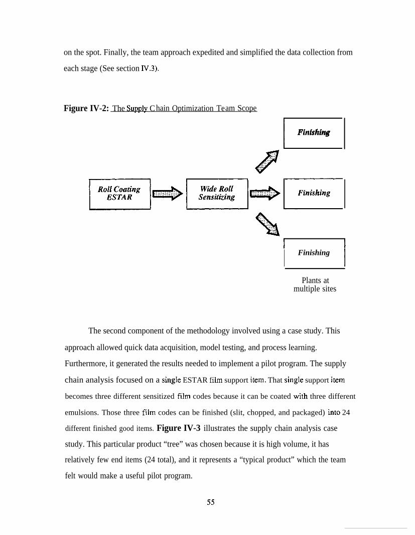
on the spot. Finally, the team approach expedited and simplified the data collection from
each stage (See section IV.3).
Figure IV-2: The Supply Chain Optimization Team Scope
EFinishing
@
,:. ,.,.: .,,.,. >,,.,:,..:.:;,: :,,.: . . . . ...,.
%
,,,.:. ,. ...>.. . . . . ...,.,:,,,.,,., .,. . . . . . .., ... .,,:..; ,.,...: :.,.:,
I Finishing
I
Plants atmultiple sites
The second component of the methodology involved using a case study. This
approach allowed quick data acquisition, model testing, and process learning.
Furthermore, it generated the results needed to implement a pilot program. The supply
chain analysis focused on a singIe ESTAR film support item. That single support item
becomes three different sensitized film codes because it can be coated with three different
emulsions. Those three film codes can be finished (slit, chopped, and packaged) into 24
different finished good items. Figure IV-3 illustrates the supply chain analysis case
study. This particular product “tree” was chosen because it is high volume, it has
relatively few end items (24 total), and it represents a “typical product” which the team
felt would make a useful pilot program.
55
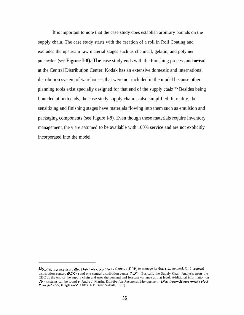
It is important to note that the case study does establish arbitrary bounds on the
supply chain. The case study starts with the creation of a roll in Roll Coating and
excludes the upstream raw material stages such as chemical, gelatin, and polymer
production (see Figure I-8). The case study ends with the Finishing process and a.mival
at the Central Distribution Center. Kodak has an extensive domestic and international
distribution system of warehouses that were not included in the model because other
planning tools exist specially designed for that end of the supply chain.35 Besides being
bounded at both ends, the case study supply chain is also simplified. In reality, the
sensitizing and finishing stages have materials flowing into them such as emulsion and
packaging components (see Figure I-8). Even though these materials require inventory
management, the y are assumed
incorporated into the model.
to be available with 100% service and are not explicitly
35K~& ~~e~ ~ ~y~tem called D1~~b~ti~n Re~~~~e~ planing (DRp) to manage its domestic network Of 5 regiOnal
distribution centers @lX’s) and one central distribution center (CDC). Basically the Supply Chain Analysis treats theCDC as the end of the supply chain and uses the demand and forecast variance at that level. Additional information onDRP systems can be found in Andre J. Martin, Distribution Resources Management: Distribution Managenten~’s MostPowerjiil Tool, (E@lewood Cliffs, NJ: Prentice-Hall, 1991).
56

Figure IV-3: SUDD .lV Chain Analvsis Case Study
Roll Coating Sensitizing FinishingSafetv Stock SafeQ Stock Safety Stick
/
Film Code 1
1
2
3
4
5
6
7
8
9
1011
Support 1
Film
!Finished Item 13
14
15
16
17
Code 2 18
19
20
\Finished Item 21/
/\Finished Item 22
\<
Finished Item 23Film Code 3
Finished Item 24
Increasing $ value
Various waste percentages
Various existing inventory levels
Typical leadtimes
57

The third component of the methodology involved using a model called Dynamic
Requirements Planning developed by Professor Stephen C. Graves of MIT’s Sloan School
of Management.3c In broad terms, the model calculates the demand and variance of
inventory (safety stock) for each stage in a supply chain. It optimizes the trade-off
between production smoothing and inventory variability given the dynamics of the supply
chain. The software model can operate either in analytic or in simulation mode. It can be
used at an aggregate level (including all of the volume flowing through each stage) or at
the item level (as with the case study product” tree” illustrated here). Advanced versions
use simulation to model push or pull systems, discrete batching, and shipping
consolidation. The team nicknamed the model the” SIP” model for Strategic Inventory
Placement. Section IV.3 and the appendix (section VII.3) provide details about the
model.
IV.3. Data Collection
Data collection represents a critical part of the supply chain analysis. Not only
does the model require detailed figures for each stage, but also the data itself can identify
potential problems in the supply chain. Once again, the team approach to the data
gathering process was essential, and team members gained a more global perspective on
their role in the supply chain.
The “SIP” model requires 4 major types of data inputs:
1. Item definition: Each item in the product “tree” requires the inputslisted in Table N-2. ~
2. Item linking: Each “branch” must be established linking items acrossthe different stages. As in a bill of materials, each “branch” includesthe waste factor for the square feet that are lost upon conversion. Theresulting “tree” structure inputs the item explosion into the model.
36T0 date, here me no ~ublicati~~~ d~taili~g tie ~~delt ~. David Kletter, a graduate student at MIT, wrote the
software and assisted with the model development.

3. Forecast variance: As described in the appendix (section VII.3), eachend item has an associated “covariance matrix. ” This input representsthe variance of the forecast from actual demand. It details forecastaccuracy 1 week ahead, 2 weeks ahead, and so on out to the planninghorizon (which is included in the Table IV-2 inputs).
4. Production smoothing: As described in the appendix (section VII.3),each item (not just end items) has an associated “weight matrix. ” Thisinput translates when downstream demand fluctuations are actuallyproduced upstream. (Thus this input is also a “wait” matrix.)
Table IV-2: “SIP” Inputs Required for Each Item in Each Stage
hits
INPUTSs Leadtime . . . . . . . . . . . . . . . . . . . . . . . . . . . . . . . . . . . . . . . . . . . . . . . . . . . . . . . . . weeks‘ Unit Cost . . . . . . . . . . . . . . . . . . . . . . . . . . . . . . . . . . . . . . . . . . . . . . . . . . . . . . . . . $/KSF*Q Inventory Holding Cost . . . . ..0...... . . . . . . . . . . . . . . . . . . . . . . Annual %● Manufacturing Frequency . . . . . . . . . . . . . . . . . . . . . . . . . . . . . . . llWeeks● Demand by End Item . . . . . . . . . . . . . . . . . . . . . . . . . . . . . . . . . . . . . . KSF/Week● Planning Horizon by End Item . . . . . . . . . . . . . . . . . . . . . . . Weekss Desired Service Level . . . . . . . . . . . . . . . . . . . . . . . . . . . . . . . . . . . . . % of periods
with no stockout* *
* KSF means Thousands of Square Feet**This is commonly referred to as Type II service
Using team participation to collect data from every stage not only proved to be
very efficient, but it also identified some potential problems in the supply chain. For
example, the model requires collection and analysis of forecast data. In the course of
using these figures, the team discovered that the forecasts contained systematic errors that
revealed potential problems with the forecasting process. Another side issue that the data
collection effort identified was a discrepancy in the Annual Operating Plan volumes
between sensitizing and finishing. The waste-adjusted numbers for the case study
product “tree” showed that Finishing intended to use more of one item than Sensitizing
planned to manufacture for it. As a result, the team learned that the annual planning
process was not connected between the two stages and relied on completely separate
59

inputs. The team subsequently formed sub-groups charged with resolving both of these
problems that the data had revealed.
IV.4. Results
The supply chain analysis showed the potential to lower inventory across the case
study product “tree” by 20%. The general intuitive principles discussed earlier were
shown to hold true, and the “SIP” model quantified the results as shown in Figure IV-4.37
Note that in general, inventories can be pushed upstream where they are in a strategic
position because:
● The inventory is common to the greatest number of finished end itemsdesired by the customer
c The inventory is at its lowest value added and thus at its lowestcarrying cost
In fact, the inventory levels of Roll Coating’s “Support 1” actually need to increase to
provide savings for the supply chain as a whole. This does not necessarily contradict the
Single Product Analysis which might suggest lowering inventory. For one thing, the
Single Product Analysis does not consider the effects of the rest of the supply chain. But
more importantly, the Single Product Analysis is designed to quantify and prioritize setup
time reduction opportunities. Subsequently, any setup time reductions can be used to
drive the “SIP” model, which then can determine the best inventoly policy for the supply
chain.
37This solution was found using the “SIP” model. Service levels were set at 9570 for each stage. The weight matriceswere not optimized and were set to reflect each stage’s lead time and manufacturing frequency. In order to reflectKodak’s current scheduling systems, there was no production smoothing across weeks.
60

Figure IV-4: Results from the SuR~Iv Chain Analvsis – Strategic Inventory Placement
Changes in $ Inventory Values
Roll Coating Sensitizing Finishinx
/
t
t+1290
support 1
Note
+50910
Film Code 1
.
M’temEEl”msmltem
1
2-12
13
! -53% t l=q’”’ 1 5 - 1 7
Film Code 2
t ~1 ‘“” 18
‘wEk:yq~1tem224 3 % Items 23-24
Excludes emulsion and chemicals inventories. Excludes regional distribution center (RDC) inventories.Includes all WIP, cycle, and in-transit stocks. Finished goods inventories are gross CDC averages.Serwce levels are at 95% for all stages. There is no production smoothing.
The definition of “inventory” as it is used in this results section is important. The
inventory changes and comparisons in Figure IV-4 represent average inventones.
Average inventory for each item includes the safety stock calculated by the “SIP” model
plus the cycle stock from aggregation needs plus the pipeline stock from transport needs.
Figure IV-5 illustrates a representative calculation for a single item. Using average
inventories to show potential reductions proved critical in convincing the Supply Chain
61

Figure IV-5: Remesentative Inventory Calculation for One Finished Good Item
Assume:● Average Demand (KSF*/Wk) 100
● 1992 Average Inventory (Days**) 38“ 1992 Average Inventory (KSF) 750
L!!L +
(Calculated from “SIP” modeltaking into account entiresupply chain)
Safety Stock (Days) 5Safety Stock (KSF) 100
CycleStock
Avg Lot Size (KSF) 200Truckload Quantity (KSF) ~Total Accumulation (KSF) 700
(Avg cycle stock= half of 700)
Cycle Stock (Days) 18Cycle Stock (KSF) 350
+Pipeline
Stock
Total Average Inventory (Days)Total Average Inventory (KSF)
Transit to Next Stage (Days)System Update Time (Days)Order Processing Time (Days)Location Setting Time (Days)
Pipeline Stock (Days)Pipeline Stock (KSF)
32630
Total Inventory Reduction (Days) 6Total Inventory Reduction (KSF) 120 (-16%)
*KSF means thousands of square feet**Kod& ~nventlon Convats weeks to days on tie basis of 5 day work weeks
Note: Pipeline times are measured in days, not hours, because the computer system updates once eachnight in a batch run
4131
9180
Sample calculations have been included for instinctive purposes. The numbrs used in tiesecalculations are not representative of actual manufacturing data.
62

Optimization Team to trust the model results. The production managers and planners on
the team could relate to average inventory numbers, especially when expressed in days,
because that is the way they are used to thinking of inventory. The team could compare
actual average inventories for 1992 with the “SIP” model’s average inventories and feel
comfortable with the magnitude of the proposed reductions. Viewed in isolation, some of
the potential reductions in safety stock were quite dramatic (60% to 80%) and prompted
one manager to comment, “These results bring acid to my stomach. ” Adding the cycle
and pipeline stocks helped dilute the safety stock reductions and gave the team
confidence to implement a pilot program based on the “SIP” model outputs.
In order to implement the “SIP” model recommendations, the team needed to feel
confident in the results. Therefore, multiple scenarios were run to test the sensitivity to
various parameters. Table IV-3 shows the sensitivity to different service level scenarios.
As service level goals at each stage are increased, the required inventory across the
supply chain must increase. This is not a linear relationship, but rather follows the
standard normal cumulative distribution function (as you approach 99.9% of the area
under the unit normal curve, you need to go out many standard deviations).
Table IV-3: SuDrIly Chain Analwis - Sensitivity to Service Level
Baseease
Potential $ Inventory ReductionAcross the Supply Chain
95%ServiceLevel
21%
97% 99%Service ServiceLevel I&@
18% 13%
Note: Results are based on the case study product “tree.”Service levels apply to all stages.
63

Table IV-3 applies the same service level across all three stages in any given scenario.
This reflects Kodak’s current way of thinking, but it is not a requirement either for the
“SIP” model or in reality. The conclusions of this thesis (Chapter V) discuss some of the
benefits and areas for future study that involve different service levels for each stage of
the supply chain.
Table IV-4 quantifies the sensitivity to different lead time scenarios. When the
lead time of any stage is reduced, the required inventory across the supply chain can also
be reduced. The “SIP” model proves very useful for translating the effect of cycle
time/lead time improvements at one stage on other stages both upstream and downstream.
Table IV-4: SuDp .lV Chain Analysis – Sensitivity to Lead time
Basecase50% of
Standard~
Potential $ Inventory ReductionAcross the Supply Chain 24V0
Note: Results are based on the case study product “tree.”
7 150% ofStandard StandardLead tim Lead time
21% [ 16%
Finishing leadtime is not halved in the 50% Leadtime” scenario due tointeger limitations in the model
Table IV-5 shows the sensitivity to different forecast variance scenarios. As the
forecast variance is reduced (improved forecasting), the inventory can be reduced.
Forecast variance here is completely independent of demand variability. That is, the
important issue is how well can demand swings be predicted, not how much is demand
fluctuating. In this particular case study, a 50% reduction in forecast variance (Table IV-
5) helps to lower inventory levels more than a 50% reduction in lead time (TabIe IV-4).
However, it may be artificial to run scenarios on these parameters separately because, in
64

general, reduced lead times will allow shorter planning horizons, and hence improved
forecasts over the lead time.
Table IV-5: SupD -lV Chain Analvsis – Sensitivitv to Forecast Variability
50% ofCurrentForecastVariance
Potential $ Inventory ReductionAcross the Supply Chain 27%
Basecase
CurrentForecastVariance
21%
150% ofCurrentForecastVariance
17%
Note: Results are based on the case study product “tree.”Taking 50% of the variance is equivalent to taking the standarddeviation divided by the square root of 2
Besides the required safety stocks, the “SIP” model also provides information on
the induced demand variance at each stage of the supply chain. This demand variance
can be used to determine the surge capability needed for any item. The calculated
demand variance is based on forecast variance, production smoothing, lead times, and the
degree of commonality for upstream items. For instance, in the case study product “tree,”
24 end item sources of variability offset each other as they get translated upstream into
the demand for one common ESTAR support item. Figure IV-6 illustrates how the
“SIP” model outputs can be used to determine the surge requirements for that one support
item.
65

Figure IV-6: Surge Requirements Examtie for Support 1
Typical Model Outputs
Scaleci DemandDemand Std. Dev.
KXll!K) ~
1,000 300
Required*Surge
Capability~
1,494
Note: KSF stands for thousands of square feet*Assumes surge capability covers 959’o (or 1.645 standard deviations) of the expected demand
No model is perfect, and no description of a model is complete without a list of
shortcomings. The “SIP” model has three weaknesses:
c It does not account for lead time variability“ It assumes stationary average demand over time
“ It cannot accommodate a large product explosion
The model assumes deterministic lead times. Once an order is placed, a finished product
appears exactly one lead time later, no earlier and no later. The long-run average demand
is fixed so that the model would have to be re-run over time to accommodate steady
increases, declines, or seasonal effects. New versions of the model incorporate actual
forecasts using simulation which can help average out these effects. Finally, the cument
version of the model cannot easily handle a product “tree” that splits into more than 25
end items. However, in most practical situations, a team should probably not be working
at any greater level of detail than this. Keeping the model at a high level both reinforces
the fundamental guiding principles and also makes decisions on implementation simpler.
66

IV.5. Implementation
Once all of the supply chain analysis requirements were complete, the stage was
set to implement a pilot program. To recap, the preparation that was in place included:
●
●
●
●
●
●
An experienced team with representatives from each stage andfunctionA complete set of data inputs validated by the teamA “basecase” set of recommended inventory levels for each stage thatthe model calculatedA set of actual inventory data to compare to the “basecase”A series of “aggressive” and “conservative” inventory scenarios to testthe model’s sensitivityA surge requirement analysis for each stage’s capacity
Armed with these data, the Supply Chain Optimization Team gathered for an all-
day session to discuss the results and decide if they felt confident enough to try the
strategic inventory placement. The team added local intelligence about specific
customers and manufacturing issues for each item that could not be captured by the
model. After reaching an understanding about how all of the model’s proposed changes
would impact the supply chain, the team decided to implement a pilot program. They
chose to follow the most conservative scenario as a starting point with the intention of
moving to the “basecase” if there were no service problems. Like a case study approach,
the pilot program could be used to test the validity of the model on a small scale with a
minimum amount of risk.
The Supply Chain Optimization Team implemented a plan for the case study
product that only involved the inventories of three items. The plan raised the one Roll
Coating item’s inventory by 20% (all safety stock), and it lowered two Sensitizing items’
inventories, each by 60%. This provided a net, one-time inventory reduction of close to
$400 K and an annual savings of close to $100 K. The plan was implemented in early
1993 so that the increase in Roll Coating inventory would not affect 1992 end-of-year
targets. The savings were captured in the 1993 Annual Operating Plan for the case study
67

line of business. As of the end of April, 1993, not a single end customer order had been
missed on the pilot product due to stockouts or inventory shortages.sg
The main barrier that the team had to overcome in reaching the implementation
stage was understanding how the “SIP” model works. The following tools helped them
build up the necessary confidence and trust in the model:
●
●
●
●
●
●
Running different scenarios, especially conservative ones
Displaying all the input data and its sources for validationExplaining how the model used the input data
Comparing the model results versus current inventory levelsShowing the required surge capacityExposing all of the model’s shortcomings
Finally, the manner and conviction with which the results are presented have a big impact
on whether an academic model and a vision of rapid customer response through the
supply chain can become a practical business reality.
The next step for the Strategic Inventory Placement model involves transferring
the methodology to other supply chains in other lines of business. The results of the pilot
test and subsequent expansion of the program can be publicized through Kodak
worldwide forums including plant cycle time coordinator conferences, the worldwide
cycle time newsletter, and the hi-weekly supply chain (“Macro-flow”) leaders meetings.
Any supply chain with a strong team, a focused set of products, and a willingness to
reduce inventory would provide a ripe environment for trying the strategic inventory
placement approach. The annual value of implementing “SIP” programs across all of the
Roll Coating - ESTAR supply chains could exceed $4 MM.
38Phone call to the Supply Chain Optimization Team leader on 4-27-93.
68

IV.6. The Springboard Effect
Another goal for the Supply Chain Analysis was to assess the impact of various
department level policies on the entire system. The Strategic Inventory Placement model
addresses this type of issue by analyzing the supply chain as a whole, and this approach
in turn highlighted an inventory management policy that has been termed the
“Springboard Effect.” In order to run the” SIP” model and interpret its results, the team
needed to understand the upstream information flows as well as the downstream material
flows. One result of studying the information flows was the discovery about the
systematic impact of setting safety stocks in weeks.
The Springboard Effect describes the way a change in downstream demand is
transmitted up the supply chain at Kodak. Basically, any forecast and demand noise is
amplified as the information is passed upstream. Demand increases trigger larger and
larger production levels upstream, and demand declines leave component inventories
stranded without orders. For example, a small increase in demand for one finished good
item might launch a growing response moving upstream in the supply chain until finally a
raw material supplier may end up doubling or tripling its production levels. Basically
there are 2 root causes behind the Springboard Effect:
1. Current scheduling algorithms set safety stocks in forward weeks ofsupply
2. Demand information is passed upstream department to department
The first root cause is that safety stock targets are measured and thought of as a
certain number of weeks. The number of weeks is translated into a real quantity based on
the immediate future demand. That is, if the safety stock target is 2 weeks and the
forecast demand is 100 in week 1,50 in week 2, and 10 thereafter, then the target safety
stock quantities will be 150 in week 1, 60 in week 2, and 10 thereafter. There is a
rationale behind this logic that says measuring targets in weeks of forward supply covers
supply variability by always producing products before they are needed. The logic builds
69
-.

in safety time.39 However, the implication of the first root cause is that forecast changes
cause safety stock quantiw changes.
The second root cause is that at Kodak, upstream stages only receive updated
demand information when their downstream customer passes it back to them. The
rationale behind this process is that each stage shifts the timing of orders around to meet
its own capacity limitations and inventory goals, and then it passes on the “filtered”
changes upstream. The implication of the second root cause is that upstreant departments
do not have visibility of the actual fin.ished goods demund changes; they only “see” a
filtered version at a later tinxe.40
These two root causes lead to the following scenario (see Table IV-6): Marketing
says finished goods demand for item Z is increasing by 50%. Because the finished goods
inventory aim is measured in weeks of forward supply, its inventory quantity must also
increase by 50%. So Finishing must now produce 5070 of what it currently has in
inventory. Finishing then dutifully passes along this information to Sensitizing. Now
Sensitizing, who also measures its inventory in folwa.rd weeks of supply, must increase
its own inventory quantity by 50% because of the demand change. Plus, it must produce
enough to cover Finishing’s inventory increase too. Therefore Sensitizing must now
produce 83% of what it currently has in inventory, 50%
downstream inventory. The springboard has started!
for itself and 33% for
Sensitizing then passes on its demand upstream to Roll Coating. Roll Coating
must now produce enough to cover its own inventory increase, as well as that of
Sensitizing and that of Finishing. Now Roll Coating must produce a colossal 125% of
what it currently has in its inventory. The springboard continues to amplify this demand
39For a description of safety time versus longer lead times and different applications of safety time, see Thomas E.Vollrnann, William L. M-r-y, and D. Clay Whybark, Manu$actw-ing Planning and Control Systems, (3rd ed.Homewood, IL: Business One Irwin, 1992), pp. 33-34 and 461-465.
40nis situation is reminiscent of the “MIT Beer Game” as described in Peter M. Senge, The Fijlh Discipline: The Artand Practice of the Lzarning Organization, (New York, NY: Doubleday/Currency, 1990). pp. 2742.
70

● ✍✎✎
change at ever increasing levels as information is passed upstream. Table IV-6 illustrates
the effects of this 50% demand increase scenario.
Table IV-6: The Springboard Effect: 50% Demand Increase Scenario
—Upstream~
Roll support~~ Coating Chemicals
Hypothetical Datu:Inv Aim (Inv Wks)Waste Factors (BOM)
4 6 8 151.00 1.20 1.44 1,58
Demand increase by 50%:Original Inventory (SF) 100 180 288 594Inventory Increase (SF) 50 90 144 297
Production for own Inv “ 50 90 144 297Production for Downstream Q m u mTotal Production 50 150 360 868
Production/Original Inv 50?Z0 83% 125% 146%
Note: The above numbers are included for instructional purposes and are not representative of actualmanufacturing data. The waste factors, for example, are just 20% compounded.
Figure IV-7 expands this single scenario to show the results of all different
forecast increases on each stage of the supply chain. If the demand for an item doubles (a
common occunence at Kodak especially on new items), the graph shows that the fourth
stage upstream will actually have to produce triple the amount it currently has in
inventory.
71
———..——. .. —.——

Figure IV-7: The !bringboard Effect for Different Forecast Increases
ProductionOriginal Inv
300%
250%
200%
150%
100%
50%
o%
.
o% 20% 40% 60% 80% 100%
Forecast IncreaseNote: The above numbers are included for instructional purposes and are not representative of actualmanufacturing data. The lines were generated from the hyp&hetical data in Table IV-6.
Of course the forecast does not always increase. When the forecast is decreased,
the Springboard Effect occurs, but in the opposite direction. Each stage’s inventory
targets go down, and upstream stages are left with inventones that will have no demand
until each downstream stage has drained its own inventories. To summarize the
Springboard Effect:
● Forecast Up means upstream stages spring to fill inventory targetsthroughout the supply chain
“ Forecast Down means stranded inventory will be slow to drain out ofthe supply chain
72
. ..- . . . .. —- . . . .
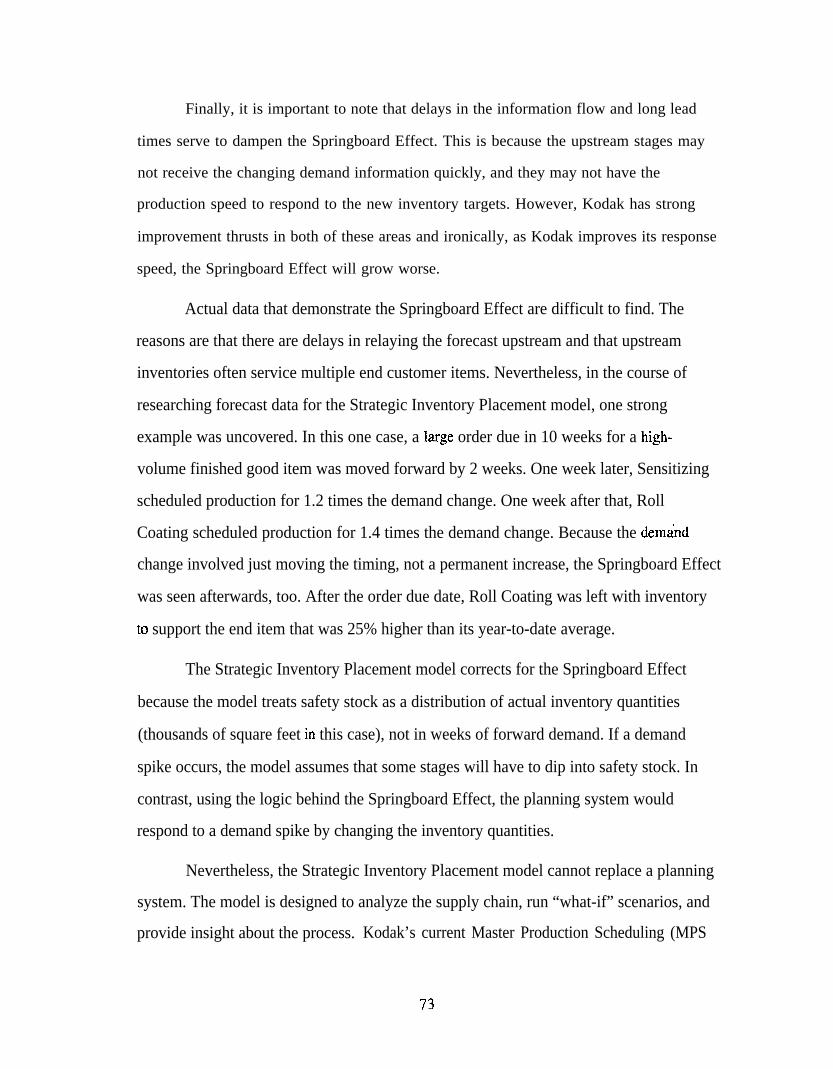
Finally, it is important to note that delays in the information flow and long lead
times serve to dampen the Springboard Effect. This is because the upstream stages may
not receive the changing demand information quickly, and they may not have the
production speed to respond to the new inventory targets. However, Kodak has strong
improvement thrusts in both of these areas and ironically, as Kodak improves its response
speed, the Springboard Effect will grow worse.
Actual data that demonstrate the Springboard Effect are difficult to find. The
reasons are that there are delays in relaying the forecast upstream and that upstream
inventories often service multiple end customer items. Nevertheless, in the course of
researching forecast data for the Strategic Inventory Placement model, one strong
example was uncovered. In this one case, a large order due in 10 weeks for a high-
volume finished good item was moved forward by 2 weeks. One week later, Sensitizing
scheduled production for 1.2 times the demand change. One week after that, Roll
Coating scheduled production for 1.4 times the demand change. Because the dern~nd
change involved just moving the timing, not a permanent increase, the Springboard Effect
was seen afterwards, too. After the order due date, Roll Coating was left with inventory
to support the end item that was 25% higher than its year-to-date average.
The Strategic Inventory Placement model corrects for the Springboard Effect
because the model treats safety stock as a distribution of actual inventory quantities
(thousands of square feet in this case), not in weeks of forward demand. If a demand
spike occurs, the model assumes that some stages will have to dip into safety stock. In
contrast, using the logic behind the Springboard Effect, the planning system would
respond to a demand spike by changing the inventory quantities.
Nevertheless, the Strategic Inventory Placement model cannot replace a planning
system. The model is designed to analyze the supply chain, run “what-if” scenarios, and
provide insight about the process. Kodak’s current Master Production Scheduling (MPS
73

II) and Materials Resources Planning (MRP II) systems are more appropriate for
managing inventones on a detailed level across the plant. One potential solution for
reducing the Springboard Effect without totally rewriting the existing inventory systems
involves redefining the way “forward weeks of supply” are counted. Instead of having a
l-week safety stock target refer to the actual next 1 week of demand, the system could
have it refer to an average rate of demand. The average rate could define a week of
safety stock as 1/52 of the year’s demand in the case of a flat market, or the average rate
could cover shorter periods if the market is seasonal. In any case, the effect on safety
stock levels of a one week demand spike would be dampened out by a factor of 1/52 or
l/season. With steadier safety stock targets, the production rates across the supply chain
could be scheduled more smoothly. Demand noise would then be dampened, rather than
amplified, moving up the supply chain.
In summary, there would be two advantages to altering the definition of “forward
weeks of supply” in this way. The first advantage is that the production swings from the
Springboard Effect could be eliminated without discarding the current systems. The
second advantage is that the safety stock targets would still change, albeit more gradually,
in response to forecast demand trends. lf an absolute safety stock quantity were fixed for
each item, then manual intervention would be required whenever any item’s long range
demand changed. Identifying and addressing issues such as the Springboard Effect
represent an important part of supply chain management, and it illustrates the value of
extending the scope of examination across the entire system.
IV.7. The Downward Production Effect
Another department level policy issue that the Supply Chain Analysis addressed
was the “Downward Production Effect.” This effect describes a situation in many Kodak
manufacturing departments where the highest production rate occurs in January. The rate
’74

gradually declines throughout the calendar year until December when the production rate
reaches its minimum. Suddenly, during the following January, the production rate jumps
again, reaching a new annual peak.
The Downward Production Effect could have adverse effects for two reasons:
● Poor asset utilization“ Poor use of labor
Basically, the effect imposes an artificial seasonality on the manufacturing process.
Capital intensive assets like the 11o11 coating machines could go unused in the latter half
of the year. New customers cannot be brought in because they could not be serviced in
the early part of the year when capacity is stretched to the limit. Moreover, enough labor
must be hired and trained (and often paid overtime) to run at full load early in the year,
and then later in the year the department becomes over-staffed.
Figure IV-8 illustrates the Downward Production Effect in a single production
area for 1990 and 1991 by using regression analysis, (1989 and earlier data were
unavailable, and 1992 could not be calculated without a full year of actual results.) The
X-axis shows one data point for each month. The Y-axis shows production as a
percentage of the monthly average for the year. Basically the Y-axis is a specific month’s
production divided by the monthly average for the year. The production rates are
adjusted for number of days in the month.41 The production area operates 24 hours per
day, 7 days per week, so weekends and holidays were included. Major mechanical
41 The adjustment for different numbers of days in the month worked in the following way:
[Adjusted Production Rate] =[DayslMonth]@(;)
. [Actual Production Rate for Month]
For example, if 100 units were actually produced in February. &en
[Adjusted Production Rate for February] = [N3[1W]= 109 adjusted units / month
75

repairs on machines were excluded. The actual production rates for the years can be
different because the analysis normalizes for different absolute quantities.
Figure IV-8: The Downward Production Effect
Note:
Slope = -1.7!% per monthII
+:--
+++ I(
III
1,, :,:: :,:: :1:::::::::::
1990 1991
● R-Squared = 42%
“ p-value= 0.05%
Monthly production is adjusted for the number of days in the month.Each year is normalized by the average daily rate.The numbers in this chart are for instructive purposes and are notrepresentative of real manufacturing data.
The meaning of Figure IV-8 is that production rates in a particular department
showed a statistically significant decline of 1.7(ZO per month over the course of each year
for two years running. The data verifies that the Downward Production Effect is real for
certain areas. A simple regression model showed a slope of 0.017 with an F-ratio of 16
(see Table IV-7). Any F-ratio higher than 7.9 (for these degrees of freedom) indicates
76
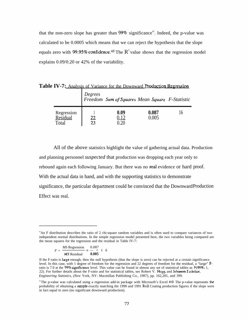
that the non-zero slope has greater than 99T0 significance42. Indeed, the p-value was
calculated to be 0.0005 which means that we can reject the hypothesis that the slope
equals zero with 99.9570 confidence.43 The R2 value shows that the regression model
explains 0.09/0.20 or 42% of the variability.
Table IV-7: Analysis of Variance for the Downward ~-~~a
DegreesFreedom Sum ojSquares Mean Square F-Statistic
Regression 1 0.09 0.087 16Residual z 0.12 0.005Total 23 0.20
All of the above statistics highlight the value of gathering actual data. Production
and planning personnel suspected that production was dropping each year only to
rebound again each following January. But there was no real evidence or hard
With the actual data in hand, and with the supporting statistics to demonstrate
significance, the particular department could be convinced that the Downward
Effect was real.
proof.
Production
42An F distribution describes the ratio of 2 chi-square random variables and is often used to compare variances of twoindependent normal distributions. In the simple regression model presented here, the two variables being compared arethe mean squares for the regression and the residual in Table IV-7:
MS Regression 0.087F = = — = 1 6
MS Residual 0.005If the F-ratio is lwge enough, then the null hypothesis (that the slope is zero) can be rejected at a certain significancelevel. In this case, with 1 degree of freedom for the regression and 22 degrees of freedom for the residual, a “large” F-ratio is 7.9 at the 997o sign~lcance level. This value can be found in almost any set of statistical tables as F(99~o; 1,22). For further details about the F-ratio and for statistical tables, see Robert V. Hogg, and Johannes Ledolter,Engineering Statistics, (New York, NY: Macmillan Publishing Co., 1987), pp. 162,281, and 399.43 The p-value was calculated using a regression add-in package with Microsoft’s Excel 4.0. The p-value represents theprobability of obtaining a sample exactly matching the 1990 and 1991 Roll Coating production figures if the slope werein fact equal to zero (no significant downward production).
77

Furthermore, additional research showed that more than one department was
experiencing this effect. In fact, in 8 out of 14 areas sampled across the supply chain,
there was a Downward Production Effect with at least a 90% significance level.
At this time, the exact causes of the Downward Production Effect have not been
determined, and it remains an opportunity for further research. However, there are two
major hypotheses:
c End of year point inventory reduction targets drive downreplenishment orders throughout the supply chain.
● Inventory build-ups preceding mechanical shutdowns occur all du~ingthe year up and down the supply chain, but are rarely scheduled duringthe November–December holiday season.
“ Sales targets are systematically high.
Either of these two causes, or a combination including the Springboard Effect is possible.
The important point is that Downward Production is a supply chain wide phenomenon.
Its damaging effects on labor and asset utilization spread when downstream stages
transmit ever-decreasing orders upstream. The role of the supply chain analysis in this
case is to manage the inventory across all the stages and to communicate clearly all of the
strategies for change. If inventories need to be reduced, then the supply chain can work
together to execute the change without disrupting production or creating detrimental
cycles. The Downward Production Effect represents yet another instance where taking a
broad perspective across the supply chain is critical.
Once the cause of the Downward Production Effect has been determined,
prospective solutions can be developed. If end-of-year point inventory targets are indeed
driving down production throughout the year, then at least two potential solutions exist:
1. Use a moving monthly average rather than an end-of-year point inperformance metrics
2. Use a supply chain-wide measure of inventory rather than measuringeach department separately
78
.

The first potential solution might measure say the average daily inventory for the last 2
months. Although improvements might take awhile to appear, this type of moving
average would eliminate some of the “game playing” that can be used to make a point
measure of inventory lower. The second potential solution would remove the incentive to
cancel orders from upstream suppliers just before the measurement date in order to make
a single department’s own books look good. In the long run, it is far more beneficial to
the company to have rapid and smooth supply chain production than a single snapshot of
low inventory.~
‘It is public knowledge that bond rating services such as Moody’s and Standard& Poor’s still use conventional end-of-year point inventones as part of their rating process. Until they change their methods, companies may have a legitimatereason to lower their production at year end to reduce inventories artificially. Companies could potentially avoid abond rating downgrade that would increase their real cost of capital.
79

80

Cha~ter V. Conclusions
V.I. Summary
Cycle time represents a vital competitive dimension for the Roll Coating Division
and for Eastman Kodak Company as a whole. Through a series of three case studies that
gradually expand in scope, this thesis has addressed cycle time reduction at every level of
detail. Each case study examined the concept of inventory levels and their effect on
production, scheduling, and cost. Inventol~ fundamentally reflects the way the business
is being run and how well it is petiorming against the competition. As Karmarkar
suggests, ” [This] question of how to determine inventory levels cuts quickly to the basics
of manufacturing in an age of intense global competition.”ds
The central themes that unite the case studies in their efforts to reduce cycle time
include:
c The need to understand the fundamental manufacturing process andincorporate that knowledge into the problem solving approach
● The importance of finding the right level of detail to address theproblem at hand
● The value of looking across the entire supply chain and recognizingthe effect that one department’s decisions can have across the system
Every case study required process understanding. Without a detailed grasp of what an
ESTAR machine setup entails, there would be no way to quantify the effect of setups on
cycle times. Every case study provided a different level of detail to answer a different
question. The Single Product Analysis could incorporate supply variability and the
Single Machine Analysis could incorporate product sequencing, but both at the cost of
not considering the impact on upstream and downstream stages. The Supply Chain
Analysis, on the other hand, lacked those fine points, but could address the broader issue
of what inventories should link the stages together. Finally, looking across the entire
45Uday S. Karmarkar, “Getting Control of Just-in-Time, “ Harvard Business Review 67:5, September-October, 1989, p.126.
81
supply chain provides tremendous leverage and global thinking toward which actions will
benefit the company as a whole.
V.2. Recommendations
On a broad level, the recommendation is to maintain and promote Kodak’s
corporate emphasis on cycle time reduction. Rapid cycle times provide a competitive
weapon for satisfying the customer, reducing cost, and improving quality. Each business,
each division, and each machine team needs to translate how the company’s cycle time
vision applies to their scope of activities. Then analysis and models such as those
presented in this thesis can help assess the impact of particular actions and prioritize
improvement opportunities.
One important obstacle that hinders cycle time improvement throughout Kodak is
the Materials Resources Planning (MRP II) system. The recommendation is to evaluate
constantly the need to have a system which constrains thinking to weekly buckets and to
fixed lead tirnes.4b How can the company encourage, measure, and reap savings from
cycle time reductions of less than a week if the systems only schedule in terms of weeks?
What incentive is there for operators or engineers to work on speeding up every setup if
tie next stage is not scheduled to consume that item until a fixed lead time has elapsed?
Thus, the recommendation is that management create greater incentives for cycle time
reduction because the whole structure of the scheduling system creates disincentives.
On a more focused level, the recommendation is to expand on the three critical
areas discussed in the thesis case studies. For the Single Product Analysis, the benefits of
setup time reduction and lot sizing can be emphasized and encouraged by applying the
46Conflicting evidence has arisen recently that part of the system is not constrained to weekly buckets. This thesis isbased on data from interviews with the master planners and their supervisors, and it represents their perception of thescheduling system’s capabilities.
82

model results to each machine team’s performance matrix. Roll Coating can also re-
energize the “pit crew” concept of choreographing setups in advance and stressing quick
changeovers. Setup time reduction appears to be the next major frontier on Kodak’s
corporate cycle time reduction strategy. Ultimately, Kodak might consider measuring
production employees on inventory as well as on waste to encourage actions that address
both issues simultaneously.
For the Single Machine Analysis, Roll Coating can always seek new ways to
optimize capacity and sequencing. New custom-designed detailed scheduling tools are
being introduced constantly and could be integrated with the existing scheduling systems
(see Figure 1-6).47 Most important, though, is to educate ESTAR employees about the
process intuition that the model provided, including the implications of
● Running at capacity
c Sequencing of products
● Speed of setups
c Flexibility of machines
Another recommendation is to resist the temptation to have a fixed product sequence and
a fixed lot size for each product. The Single Machine Analysis showed that these
parameters should remain flexible and respond to the entire load on the system. Finally,
the concept of increased flexibility, (any machine running any product without long
setups), could provide a fundamental solution that removes the scheduling complexity
instead of merely coping with it.
For the Supply Chain Analysis, the recommendation is to roll out the results of the
pilot program across the entire product line of business studied. Moreover, the concept of
strategic inventory placement could be applied to other film lines and even Kodak’s other
47For ~ ~evlew of det~led ~~hedul~g packages, see Uday S. Karmarkar and Milind M. Le~e. “me Marketin/Y
Manufacturing Interface: Strategic Issues.” University of Rochester Center for Manufacturing & OperationsManagement Working Paper Series, CMOM 89-10$1991, p.1.3.
83

non-photographic businesses. The Supply Chain Analysis involved acultural shift where
the team was focused on their role as members of a product “flow” serving the end
customer. This supply chain allegiance challenges many companies’ traditional
organizational focus on fimctions or single departments. A recommendation would be to
expose everyone associated with products, operators and engineers, to the business unit
goals and the other members of their supply chain.
Another supply chain recommendation is to gather and publicize some of the data
that the SCOT team collected even if it is not going to be input into the “SIP” model. The
forecast variance data can detect systematic forecast process problems, and the
comparison of each stage’s demand data can pinpoint any disconnects in the Annual
Operating Plan.
To combat the Springboard Effect, the recommendation is to communicate end
item demand changes to every stage in the supply chain without delay. Also, with a
small systems change, safety stocks could be based on demand rates of a year or a season,
rather than on immediate forward weeks of supply, These actions would help darnpen
out the demand noise amplification that currently causes large swings in upstream
production requirements.
For the Downward Production Effect, if it is indeed caused by end-of-year point
inventory targets, then the measurements should be changed. Using moving average
inventories and supply chain-wide totals might eliminate the inefficient production
declines that occur throughout the year.
One final recommendation would be to make the critical cycle time issue explicit
in the Roll Coating Division’s Vision and Mission statements. Although the statements
cover quality, teamwork, and continuous improvement, there is no mention of speed or
response time. Top management commitment is required to drive major change within
the organization, and cycle time improvement is no exception.
84

V.3. Opportunities for Future Work
The ultimate cycle time vision foresees a supply chain capable of blasting goods
through to respond to customer needs with the barest amounts of inventory between each
stage. Opportunities for future work all involve ways of transforming this vision into
reality. One paradigm worth challenging is the idea that Roll Coating, Sensitizing, and
Finishing all need to be separate functions de-coupled with inventory. Perhaps a future
state would couple these stages and provide a synchronous manufacturing process. A
similar alternative might involve a hybrid push-pull system where inventories could be
“pushed” to a strategic de-coupling point?8 and then “pulled” rapidly through the supply
chain in response to specific customer orders.
Another opportunity across the supply chain would be to explore the benefits of
differentiated service levels. Rather than providing 95% service at evely stage, a strategy
could be to provide lower service levels upstream and higher service levels downstream
to the end customer. The “SIP” model provides an ideal tool for simulating the effect of
different service level strategies on cost and delivery performance throughout the supply
chain.
Other opportunities for future work on the topics addressed by this thesis include:
c Incorporating more aspects unique to Kodak into the Single ProductAnalysis. These would include discarded product being correlatedwith lots, waste learning curves associated with each run, andsequencing effects.
s Adding lead time variability to the Supply Chain Analysis
● Finding other data-driven examples of the “Springboard Effect” andrunning simulations to test different safety stock strategies
● Testing the “Downward Production Effect” comelation to differentfactors to determine its precise cause
480r a point at which product proliferation occurs
85

Another opportunity for future work is to put the responsibility for cycle time .
reduction in the hands of the operators. As the people closest to the detailed work, they
are in the best position to eliminate non-value added transactions, streamline procedures,
and improve production techniques. They can then control other cycle time areas such as
work-in-process inventory and work queues:
Let’s stress it again. The setting of a buffer [inventory] length involves the most fundamentalmanagerial decision– the trade-off between the measurements. When choosing long buffers itdirectly impacts the level of time-related INVENTORY (work-in-process and finished tasks). . . .Choosing short buffers directly impacts . . . THROUGHPUT (unreliable delivery). Who shouldmake this decision, who should establish the length of the TIME BUFFERS? In most companies,it’s not the top manager or even the scheduler, it’s the forklift driver.49
The goal of this thesis was to address the critical issue of cycle time and its related
inventory component. The final measure of its success will be if it stimulates the reader
to think of future opportunities to apply this work to practical business situations.
49Eliy~u M. Gol&.a~t, T}le Hav~ta~k sv~rolne: Slfiing lnfo~nation Oltt of the Data Ocean, (Croton on Hudson, NY:
North River Press, 1990), p. 126. “
86

ChaDter VI. Amendices
VI.1. Single Product Analysis
The Single Product Analysis uses a Lot Size–Reorder Point system to determine
optimum operating policies50. In short, this type of system determines operating policies
by specifying when to order and how much to order. Those two pieces of information
can be used to calculate the expected manufacturing frequency, average inventory, safety
stock, and other parameters.
ln the model, both the periodic demand and the lead time are taken as variable,
and their distributions are combined to determine the resulting distribution of demand
over the lead time. The overall technique involves calculating an initial lot size using an
Economic Production Quantity formula. Then that value is used to calculate the reorder
point, which, in turn, can be used to calculate a more accurate lot size. The Single
Product Analysis repeats this iterative process once because in most cases the values
quickly converged to less than a 10% spread.
The first part of the model transforms raw data into the inputs needed to calculate
‘the lot size and reorder point. This first part involves four steps:1. Calculating the expected demand during the lead time and its standard
deviation2. Calculating the cost per setup3. Calculating the inventory holding cost4. Calculating the net production rate
50For a detailed account of this kind of system, see Thomas E. Vollrnann, William L. Berry, and D. Clay Whybmk,Mamfacturing Planning and Control Systems, (3rd ed. Homewood, IL: Business One Irwin, 1992), pp. 728-729.Another source is Steven Nahmias, Production and Operations Analysis, (Homewood, IL: Richard D. Irwin, Inc.,1989), p. 194ff.
87

1.
i?, =+.o;+ll’. t?:
~ = Expected demand during the lead time in KLF *
86 = Standard deviation of demand during the lead time in KLF
D = Mean periodic demand in KLF / Week
T = Mean lead time in Weeks
ti* = Standard deviation of periodic demand in KLF / Week
ti, = Standard deviation of lead time in Weeks
* KLF symbolizes thousands of linear feet
S = Setup cost in $ / setup
t = Setup time in minutes
M = Machine speed in linear feet/ minute
CU = Unit cost in $ / linear foot
3.
[1cHecc1 = 1,000” —
52 u
C, = Inventory cost in $/ KLF / Week
CH = Annual inventory holding cost as a % of unit cost
C’u = Unit cost in $/ linear foot
88

Note that determining CH is a calculation requiring multiple inputs that may vary
depending on the exact situation. For the Single Product Analysis, the following holding
cost factors were included:sl●
●
●
●
●
c
●
●
●
●
e
Weighted cost of capitalTaxesInsuranceSpoilageTheftObsolescenceWarehouse employee costsWarehouse space and utility costsWarehouse supplies including light-tight boxesCores atthe center oftherollsofESTAR film baseVariable inventory management costs (systems and employees)
4.
‘=y”MO[’0:::~71P = Net production rate in KLF / week
Y = Yield off of machine in YO
M = Machine speed in linear feet/ minute
~ 1 Additional ~ea~ent of inventow holding ~o~ts can be found in Barry Renden and Ralph M. Stair, Jr., Quanfifative
Analysisfor Management., 4th cd., (Boston, MA: Allyn and Bacon, 1991).
89
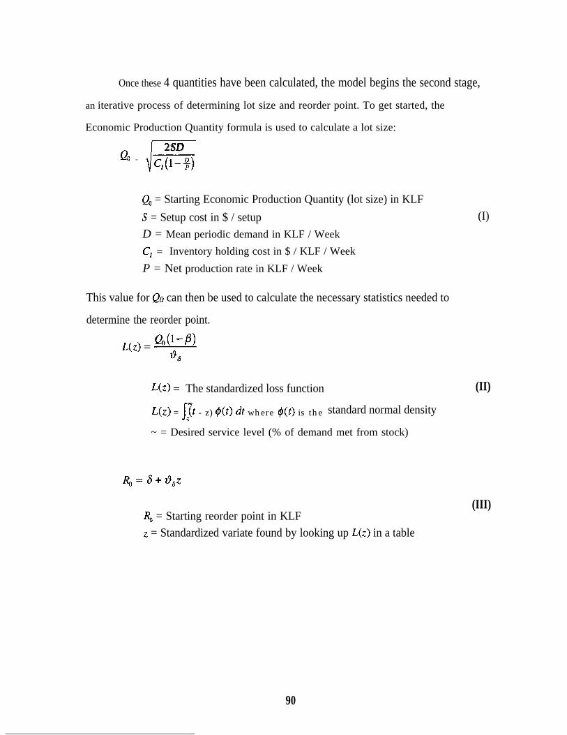
Once these 4 quantities have been calculated, the model begins the second stage,
an iterative process of determining lot size and reorder point. To get started, the
Economic Production Quantity formula is used to calculate a lot size:
Qir
2SD= Cl(l-+)
~ = Starting Economic Production Quantity (lot size) in KLF
S = Setup cost in $ / setup (I)
D = Mean periodic demand in KLF / Week
C1 = Inventory holding cost in $ / KLF / Week
P = Net production rate in KLF / Week
This value for Qo can then be used to calculate the necessary statistics needed to
determine the reorder point.
L(z) = The standardized loss function
Uz) = ~~t - z) $(t) d where @(t) is thez
(II)
standard normal density
~ = Desired service level (% of demand met from stock)
l$=&+ti6z
~ = Starting reorder point in KLFT = Standardized variate found by looking up L(z) in a table*
(III)
90

Once the first iteration values of Q. and RO have been calculated, they can be
used to determine statistics needed for another lot size iteration.
n(R) = ~(1 –
n(R) =
n(R) =
P)
Expected number of stockouts per manufacturing cycle (IV)
[;(~-R)f(~)~~whe~~(~) istheno~maldensitYfunction
F(z) = Standard normal cumulative distribution function iv-l(The probability of being to the left of z)
\vJ
These statistics allow the model to calculate the second (and final) iteration values for lot
size and reorder point.
Q,=,::;,)+{-
(21 = Lot size in KLF after iteration
~ and ZI represent the new values after iteration
RI = 6+- t?dzl
Rl = Reorder point in KLF after iteration
(VI)
(VII)
(VIII)

The values of Ql and RI now enable the model to calculate the desired operational
results in an implementable format.
Q,= Lot size in KLF
()Q, .7 = Lot size in days of production7
Q,— = Avg time between lots in weeksD
(-)SD .52= Annual setup cost in $Q1
RI – 6 = Safety stock in KLF
RI-6— = Safety stock in weeks
D
(R,-a)+~(l-;)= Average inventory in KLF
(R1-6)+Q, ~ D().— = Average inventory in WeeksD ZP
(IX)
(x)
(XI)
(XII)
(XIII)
(XIV)
(xv)
(XVI)
[Avg Inv in KM?]o Cl .S2 = Annual inventory holding cost in $ (XVII)
92

Figure VI-1 shows a sample page of a model printout.
Figure VI-1: Sinde Product Analysis SamD le Printout
Representative
INPUTSDemand Mean KLF/wk
Std Dev KLF/wkLead Time Mean wk
Std Dev wk1. Demand during LT Mean KLF
Std Dev KLF
2. Setup Cost MachineSU Time minMach speed LF/minUnit cost $ILFSetup cost $/Setup
3. Inventory Cost Annual %Weeks/yearUnit cost $/LFInv cost $/KLF/wk
4. Production Rate Mach speed LF/minYield % yieldRate KLF/wk
Desired Service Level
CALCULATIONSEconomic Order Quantity KLF
Standardized Loss FunctionStandardwed Z Value Std Dev.sReorder Point KLF
Expected stockouts per mfg order1- F(z) ~rob of being to right of z]
E.O.Q. (1st iteration) KLF
New Standardized Loss FunctionNew Standardized Z Value Std Dev.sReorder Point (1st iteration) KLF
Value of no shortfall $/K.LFValue of no shortfall $IK Sq ftInv level when order placed KLF
Product
4001002.00.5800245
30330
200$0.25
$1,500
35%52
$(-J~5$1.68
20090%
1,814
97%
956
0.11710.82
1,001
29~0.670
1,106
0.13540.74981
$23
$5981
93

Figure VI-1: Sinde Product Analvsis Sample Printout (Continued)
RepresentativeEW@!.1 l?l@!K!
MODEL RESULTS
Lot SizeLot SizeAvg Tne Between RunsSetup Cost
Safety StockSafety StockAverage InventoryAverage InventoryInventory Holding Cost
ACTUAL DATA
30 Wk Average Inventory
KLFDaysweeks$/year
KLFweeksKLFweeks$/year
KLF30 Wk Minimum Inventory IUF
#of SetupsProduction KLF#of Weeks
ACTUAL RESULTS (30 Weeks of 1992)
Lot Size KLF
Lot Size DaysAvg Tme Between Runs weeksSetup Cost $/year
Safety Stock KLFMinimum Inventory weeksAverage Inventory KLFAverage Inventory weeksInventory Holding Cost $/year
Actual minus Model Setup Cost/YrActual minus Model Inv Cost/YrActual minus Model Total CostATr
I xxXIXII
x v
XVH
1,1064.32.8
$28,216
1810.56121.5
$53,572
1,350308
109,974
30
1,500
5.83.8
$20,800
4001.0
1,5003.8
$131,250
-$7,416$77,678
$70~62
The Single Product Analysis was actually calculated using Microsoft’s Excel 4.O
spreadsheet program on an Apple Macintosh IIsi personal computer.
94

VI.2. Single Machine Analysis
The Single Machine analysis uses integer programming to determine the
minimum cost necessary to meet a given demand. The model is formulated as follows:
Definition of
Pik =
Ik =Si.. =
=
Decision Variables:
Amount of product i (in KLF) produced in week k
Amount of product ~ (in KLF) in inventory at the end of week k
1 if product i is setup from productj in week k
O otherwise
Definition of Data Variables:
CG = Cost in $ of setting up product i from product j
hi = Holding cost in $ of keeping product i in inventory for one week
ti = Tiie in hours to setup product i from productj
di~ = Demand in KLF for product i in week k
Objective Function:
Minimize cost of all setups and inventory holding:Min ~~~c~sV, + ~~hi~k
kji k i
Constraints:
1. Production and inventory balance with demand for each product and for each week:
for all i, k
2. Setup time plus production time do not exceed capacity in any week:
95

3. If a product is not setup in a given week, that product cannot be produced:P,, <ME Stik for all i, k
]
4. If the machine is setup for a given product, then a different product must be setup thatweek or the run must continue into the following week:
2fsik ‘Es,,, ‘s,,l,+l for all i, ks j*i
5. The machine can start the week set on only one product:
z S,,~ S 1 for all ki
6. The model must generate a feasible sequence of products each week:
s~, + sji~
<1 for all i#j, j#i, k
7. The starting inventory levels are input:
1.to = constant for all i
8. Safety stock and seasonal smoothing are set through the ending inventory levels:
I14 = constant for all i
9. The machine starts setup on one product. Here it is product 1:
sm~l
10. The machine does not start setup on any of the other products:~s,,, =0 foralli#l, k=l
i
11. The setup variable must be an integer O or 1. Either the setup occurs or it does not:
s,j, = 0,1 for all i, j, k
96

12. Theproduction andinvento~ mounts cannot beless than zero:
Pik, I&20 for all i, k
The Single Machine Analysis was actually calculated using Schrage’s LHVDO
program52 on an Apple Macintosh IIsi personal computer.
52Linus Schrage, LINDO: An Optimization Modeling System, (4th Ed. San Francisco, CA: The Scientific Press,1991).
9-7

VI.3. Supply Chain Analysis
This appendix will detail how the two matrices in the Strategic Inventory
Placement (“SIP”) model are defined, and then it will provide additional information on
how the model calculations work.
VI.3.I. The Covariance Matrix
The covariance matrix represents the forecast error entering the supply chain.
Each stage 1 end item has a covariance matrix associated with it. Figure VI-2 illustrates
a typical covariance matrix used in the Supply Chain Analysis. The matrix is square, and
it has 11 rows and columns which reflect the 10 week forecast horizon input for that
particular item. (The counting starts with the current week as zero, so 10 weeks plus
week zero give 11 rows and columns.) Each element represents the variance or
covariance of forecast from actual demand a certain number of weeks in advance. Only
diagonal variance elements were used in the Supply Chain Analysis. The off-diagonal
elements represent covariances, the correlation of the forecast error in one week to errors
in other weeks. The team did not use the off-diagonal columns in the Strategic Inventory
Placement analysis because the team felt that this data would not have a large impact on
their irnplementation decision.
98

Figure VI-2: The Cova.riance MatrixVariance of
Fcst 1 Wk Out
\Variance of Forecast X Weeks Out
99

In order to calculate the actual values for the covariance matrix, the following
steps need to be taken:
1. A sample of forecasts for the end item must be collected. Bydefinition, these forecasts extend out the same number of periods asthe planning horizon. Figure VI-3 depicts a sample of 10 forecasts forone end item with a 5-week horizon.
Figure VI-3: Sanmle of 10 five-week Forecasts
Week Being Forecasted:
MIZUI.E 2QU222224252622 28292!2Week of
IIQL!f@1. 16
2. 17
3. 18
4. 19
5. 20
6. 217. 22
8. 239. 24
10. 25
A F1 F2 F3 F4 F5A F1 F2 F3 F4 F5
A F1 F2 F3 F4 F5A FI F2 F3 F4 F5
A F 1 F 2 F 3 F 4 F 5
A F1 F2 F3 F4 F5A F 1 F 2 F 3 F 4 F 5
AF1F2F3F4F5A F1 F2 F3 F4 F5
A F 1 F 2 F 3 F 4 F 5
A = Actual demand for that weekF1 = Forecast for 1 week outF2 = Forecast for 2 weeks outF3 = Forecast for 3 weeks outF4 = Forecast for 4 weeks outF5 = Forecast for 5 weeks out
100

2. Next differences between the current forecast and the prior week’sforecast must be calculated for each number of weeks-out. (Note thatfor the forecast 1 week out, the prior week’s forecast is really the actualdemand that occurred.) Figure VI-4 shows, for forecasts 1 week out,how the differences from actual would be found. Figure VI-5 shows,for the forecasts 3 weeks out, how the differences from 2 weeks outwould be found.
Figure VI-4: Differences From Actual for l-Week Out Forecasts
Week Being Forecasted:
1.
2.
3.
4.5.6.7.
8.
9.
10.
Week of!lQllQQ
16
1718
1920
2122
23
24
25
F5
F4F3F2
F1
F5F4F3
F2
F5F4
F3
F5
F4 F5
Figure VI-5: Differences From Actual for 3-Week Out Forecasts
Week Being Forecasted:
MIZML92Q2U2232425M2Z 24223)
1.
2.
3.
4.
5.
6.
7.
8.
9.
10.
Week ofl@x?Q
16
17
18
1920
212223
24
A F1
A
F5F4F3
F5
F4 F5
101

3.
4.
From step 2, a set of differences has been collected for each forecast,that is, a set of differences from the forecasts 1 week out, a set ofdifferences fi-om the forecasts 2 weeks out, etc. In step 3, the samplevariance of the set of differences for each time period must becalculated. For instance, from Figure VI-5, one can obtain a set of 7differences horn actual 3 weeks out. The sample variance of this set of7 values maybe calculated from the following statistical formula:
S 23 Wksout =~~(X,-Z~—
1-
where n = 7
S2 = the sample variance
Xi = one of the sample differences– = the average “difference”x
Finally, the sample variance, represented as one single number, can beplaced in the covariance matrix; In the case illustrated here, the 3-week out forecast variance would be put in as element 3,3 in thecovariance matrix.
Gathering forecast variance data such as the inputs required for the “SIP” model
would probably have a beneficial side effect in almost any application. The analysis
requires an evaluation of past forecasts. In the particular case study business supply
chain, the forecast error was not routinely measured. Gathering data for the “SIP” model
revealed a systematic bias in the average forecast and an unexpected increase in the
variance in weeks 3 and 2 before the due date. The result was that part of the Supply
Chain Optimization Team initiated a thorough study of forecast techniques and ongoing
performance measures.
VZ.3.2. The Weight Matrix
As the Strategic Inventory Placement model was used in this thesis, the weight
matrix translates when desired production changes are actually fulfilled. In other words,
the weight matrix determines production smoothing. The basic model itself can optimize
the weight matrix to achieve the minimum cost trade-off between smoothing production
102

and avoiding inventory build-ups. As applied to the Supply Chain Analysis, the weight
matrix was used to build in delays in responding to demand changes, not for production
smoothing.
Figure VI-6 shows an example of a weight matrix used for one of the Sensitizing
items. Each item in every stage has an associated weight matrix. The columns represent
the week when a production change is desired, starting with week O (the present) and
extending out to the forecast horizon minus the sum of lead times of downstream stages.
The rows represent when the demand change is actually produced by the factory. For
instance, a 1 in column 5 and row 6 means that 100V0 of the demand change in week 4
will be start production in week 5 (counting starts with week 0). Similarly, a 0.5 in
column 8 and row 7 means that 5090 of the demand change in week 7 will start
production in week 6.
Figure VI-6: The Weight Matrix
L T = 3 w k s ~
I
Time When Desired Production Changes
Coated OnceEvery 2 Wks
103
Note that in Figure VI-6, all the rows inside the lead time must be zero. This
means that the manufacturing stage cannot accommodate demand changes inside the lead
time and must produce any additional requirements at a later time. Also illustrated in
Figure VI-6 is a production response delay every other week to represent a
manufacturing frequency of once every two weeks. This is only a delay in response to
demand changes and does not preclude production in any given week. This zero-one
pattern represents the actual inputs used to generate the Supply Chain Analysis. Later
versions of the model can handle manufacturing frequency, batch sizing, and shipping
consolidation using a simulation approach.
VZ.3.3. “SIP” Model Calculations
The Strategic Inventory Model characterizes inventory as a random variable and
determines its statistical variance. In particular, the more production is smoothed (i.e.
lower production variance), the higher will be the variance of the inventory. The safety
stock level is then set to be the mean inventory level for which the probability of stocking
out equals one minus the desired service level. As an example, if the variance of
inventory is 100, the standard deviation is 10, and the safety stock could be set at 16.45
(1.645 standard deviations) to achieve 95% service. This means the expected value of
safety stock would be 16.45, but it will vary around this mean level. 9“5~0 of the time,
however, the safety stock should stay above zero (stockout level).
the
104

Chapter VII. Biblio~raR~y
1.
2.
3.
4.
5.
6.
7.
8.
9.
10.
11.
12.
13.
14.
15.
16.
17.
Bemelmans, Roland. “The Capacity Aspect of Inventories.” In LectureNotes on Economics and Mathematical Systems. Beckmann, M. andKrelle, W., managing eds. Berlin: Springer-Verlag, 1986.
Corey, E. Raymond, ed. MBA Field Studies: A Guide for Students andFaculty. Boston, MA: Harvard Business School Publishing Division,1990.
Dertouzos, Michael L., Lester, Richard K., and Solow, Robert M. MadeIn America. Cambridge, MA: The MIT Press, 1989.Eastman Kodak Company. Quality Leadership Process Guidebook.1990.
Ford, Henry. Today and Tonzorrow. Cambridge, MA: Productivity Press,1988.
Goldratt, Eliyahu M. The Haystack Syndrome: Sifling Information Out ofthe Data Ocean. Croton on Hudson, NY: North River Press, 1990.
Graves, Stephen C. “Safety Stocks in Manufacturing Systems.” NewYork, NY: Elsevier Science Publishing Co., Inc., 1988.Graves, Stephen C. and Jordan, William C. “An Analytic Approach forDemonstrating the Benefits of Limited Flexibility.” General MotorsResearch Publication GMR-7341, 1991.
Hogg, Robert V. and Ledolter, Johannes. Engineering Statistics. NewYork, NY: Macmillan Publishing Co., 1987.
Karmarkar, Uday S. and Lele, Milind M. “The Marketing/ ManufacturingInterface: Strategic Issues.” University of Rochester Center forManufacturing & Operations Management Working Paper Series, CMOM89-10, 1991.
Karmarkar, Uday S. “Getting Control of Just-in-Time. ” HarvardBusiness Review. 67:5, September-October, 1989. pp. 122-131.
Imai, Masaaki. IL41ZEN: l%e Key to Japank Competitive Success. NewYork, NY: Random House Business Division, 1986.Jutte, Christine N. Lead Time Reduction for Multiple Step Batch ChemicalProcesses. MIT Master’s Thesis, 1992.
Knight, Thomas P. Inventory Reduction in a Large Job Shop. MITMaster’s Thesis, 1992.
Koetje, Bradley A. Improving Cycle Times in Batch ChemicalOperations. MIT Master’s Thesis, 1991.
Martin, Andre J. Distribution Resources Management: DistributionManagement Most Power@ Tool. Englewood Cliffs, NJ: Prentice-Hall,1991.
Mock, Theresa Lai-Hing. Reducing Process Variability in ChemicalBatch Manufacturing. MIT Master’s Thesis, 1992.
—— .-— -
105
.-. . . .-. —..-

18.
19.
20.
21.
22.
23.
24.
25.
26.
27.
28.
29.
30.
31.
Nahmias, Steven. Production and Operations Analysis. Homewood, IL:Richard D. Irwin, Inc., 1989.Neale, J. J. Cycle Time Reduction: A Balanced Approach. EastmanKodak Company, 1991.
Papouras, Christopher P. Lead Time and Inventory Reduction in BatchChemical Manufacturing. MIT Master’s Thesis, 1991.
Renden, Barry and Stair, Ralph M., Jr. Quantitative Analysis forManagement., 4th ed. Boston, MA: Allyn and Bacon, 1991.Schrage, Linus. LINDO: An Optimization Modeling System. 4th Ed. SanFrancisco, CA: The Scientific Press, 1991.Senge, Peter M. The Fifih Discipline: Z?e Art and Practice of theLeamin.g Organization. New York, NY: Doubleday/Currency, 1990.
Shingo, Shigeo. A Revolution in Manufacturing: the SMED System.Cambridge, MA: Productivity Press, 1985.
Stalk, George, Jr., Hout, Thomas M. Competing Against Time: HowTime-Based Competition is Reshaping Global Markets. New York, NY:The Free Press, 1990.
Thomas, Philip R. Competitiveness Through Total Cycle Time. NewYork, NY: McGraw-Hill, Inc., 1990.Toscano, Diane M. “A Tip for Survival: Manage the Supply Chain” inAPICS – The Performance Advantage, October, 1992, pp. 35–36.
Vollmann, Thomas E., Berry, William L., Whybark, D. Clay.Manufacturing Planning and Control Systems. 3rd ed. Homewood, IL:Business One Irwin, 1992.Winston, Wayne L. Introduction to Mathematical Programming:Applications and Algorithms. Boston, MA: PWS-Kent Publishing Co.,1991.
J. Wolfmann. “Report on the Photographic& Imaging Industry in theUnited States.” Popular Photography. December, 1990.Womack, James P., Jones, Daniel T., and Roos, Daniel. The Machine thatChanged the World. New York, NY: Rawson Associates, 1990.
106