CVP Analysis
60
COST-VOLUME-PROFIT ANALYSIS CHAPTER 3 Cost Accounting: A managerial emphasis By: Horgren, C., Foster, G., and S. Datar GROUP 3 : Ecleo, D., Ongy E., and A. Tulin
-
Upload
elvieentero -
Category
Documents
-
view
19.809 -
download
7
description
ELVIRA E. ONGY
Transcript of CVP Analysis

COST-VOLUME-PROFIT ANALYSIS
CHAPTER 3
Cos
t A
ccou
ntin
g: A
man
ager
ial e
mph
asis
By:
Ho
rgre
n,
C.,
Fo
ste
r, G
., a
nd
S.
Da
tar
GROUP 3 :
Ecleo, D., Ongy E., and A. Tulin

COST-VOLUME-PROFIT ANALYSISCHAPTER 3
Learning Objectives:1. Understand basic cost-volume-profit (CVP) assumptions
2. Explain essential features of CVP analysis
3. Determine the break-even point and output to achieve target operating income
4. Incorporate income tax considerations into CVP analysis
5. Explain the use of CVP analysis in decision making and how sensitivity analysis can help managers cope with uncertainty
6. Use CVP analysis to plan costs
7. Apply CVP analysis to a multiproduct company
8. Adapt CVP analysis to multi cost drivers situations
9. Distinguish between contribution margin and gross margin
Cos
t A
ccou
ntin
g: A
man
ager
ial e
mph
asis
By:
Ho
rgre
n,
C.,
Fo
ste
r, G
., a
nd
S.
Da
tar

COST-VOLUME-PROFIT ANALYSISCHAPTER 3
Objective 1
Cost-Volume-Profit Assumptions and Terminology
1. Changes in the level of revenues and costs arise only bec. of changes in the number of product (or service) units produced and sold.
2. Total costs can be divided into a fixed component and a component that is variable with respect to the level of output.
3. When graphed, the behavior of total revenues and total costs is linear in relation to output units within the relevant range (and time period).
Cos
t A
ccou
ntin
g: A
man
ager
ial e
mph
asis
By:
Ho
rgre
n,
C.,
Fo
ste
r, G
., a
nd
S.
Da
tar

COST-VOLUME-PROFIT ANALYSISCHAPTER 3
Objective 1
4. The unit selling price, unit variable costs, and fixed costs are known and constant.
5. The analysis either covers a single product or assumes that the sales mix when multiple products are sold will remain constant as the level of total units sold changes.
6. All revenues and costs can be added and compared without taking into account the time and value of money.
Cos
t A
ccou
ntin
g: A
man
ager
ial e
mph
asis
By:
Ho
rgre
n,
C.,
Fo
ste
r, G
., a
nd
S.
Da
tar

COST-VOLUME-PROFIT ANALYSISCHAPTER 3
Objective 1
Operating income = Total revenues – Cost of goods sold andfrom operations and operating costs
(excluding income taxes)
NET INCOME = Operating income – Income taxes
NET INCOME = operating income + nonoperating revenues (such as interest revenue) – nonoperating costs – income taxes
Back to learning objectivesCos
t A
ccou
ntin
g: A
man
ager
ial e
mph
asis
By:
Ho
rgre
n,
C.,
Fo
ste
r, G
., a
nd
S.
Da
tar

COST-VOLUME-PROFIT ANALYSISCHAPTER 3
Objective 2
Essentials of Cost-Volume-Profit Analysis
EXAMPLE:
Mary Frost plans to sell Do-All Software, a home office software package, at a heavily attended two-day computer convention in Chicago. Mary can purchase this software from a computer software wholesaler at $120 per package with the privilege of returning all unsold units and receiving a full $120 refund per package. The units (packages) will be sold at $200 each. She has already paid $2,000 to Computer Conventions, Inc., for the booth rental for the two-day convention. Assume there are no other costs. What profits will Mary make for different quantities of units sold?
Cos
t A
ccou
ntin
g: A
man
ager
ial e
mph
asis
By:
Ho
rgre
n,
C.,
Fo
ste
r, G
., a
nd
S.
Da
tar

COST-VOLUME-PROFIT ANALYSISCHAPTER 3
Cos
t A
ccou
ntin
g: A
man
ager
ial e
mph
asis
By:
Ho
rgre
n,
C.,
Fo
ste
r, G
., a
nd
S.
Da
tar
Objective 2
ANALYSIS:
Fixed costs = $2,000 -----booth rental
Variable costs = $120 -----cost of the package
Unit selling price = $200
Mary can use CVP analysis to examine changes in operating income as a result of selling different quantities of software packages.
The only numbers that change in selling different quantities of packages are: (1) total revenues and (2) total variable costs.

COST-VOLUME-PROFIT ANALYSISCHAPTER 3
Cos
t A
ccou
ntin
g: A
man
ager
ial e
mph
asis
By:
Ho
rgre
n,
C.,
Fo
ste
r, G
., a
nd
S.
Da
tar
The difference between total revenues and total variable costs is contribution margin. OR
Contribution margin = contribution margin per unit X number of packages sold
Objective 2
The difference between the selling price and the variable cost per unit is the contribution margin per unit.
Contribution margin per unit divided by the selling price is what we call the contribution margin percentage.

COST-VOLUME-PROFIT ANALYSISCHAPTER 3
Cos
t A
ccou
ntin
g: A
man
ager
ial e
mph
asis
By:
Ho
rgre
n,
C.,
Fo
ste
r, G
., a
nd
S.
Da
tar
Objective 2
Back to learning objectives
Number of Packages Sold
0 1 5 25 40
Revenues at $200 per package $0 $200 $1,000
$5,000 $8,000
Variable costs at $120 per package 0 120 600 3,000 4,800
Contribution margin at $80 per package 0 80 400 2,000 3,200
Fixed costs 2,000 2,000 2,000 2,000 2,000
Operating income $(2,000)
$(1,920)
$(1,600) $0 $1,200
Contribution Income Statement for Different Quantities for Do-All Software Packages Sold
Spreadsheets computation

COST-VOLUME-PROFIT ANALYSISCHAPTER 3
Cos
t A
ccou
ntin
g: A
man
ager
ial e
mph
asis
By:
Ho
rgre
n,
C.,
Fo
ste
r, G
., a
nd
S.
Da
tar
Objective 3
The Break-Even Point
The break-even point is that quantity of output where total revenues equals total costs – that is, where the operating income is zero.
Why would managers be interested in the break-even point?

COST-VOLUME-PROFIT ANALYSISCHAPTER 3
Cos
t A
ccou
ntin
g: A
man
ager
ial e
mph
asis
By:
Ho
rgre
n,
C.,
Fo
ste
r, G
., a
nd
S.
Da
tar
Objective 3
Abbreviations used in the subsequent analysis:
USP = Unit selling price
UVC = Unit variable costs
UCM = Unit contribution margin (USP-UVC)
CM% = Contribution margin percentage (UCM/USP)
FC = Fixed costs
Q = Quantity of output units sold (and manufactured)
OI = Operating Income
TOI = Target operating income
TNI = Target net income

COST-VOLUME-PROFIT ANALYSISCHAPTER 3
Cos
t A
ccou
ntin
g: A
man
ager
ial e
mph
asis
By:
Ho
rgre
n,
C.,
Fo
ste
r, G
., a
nd
S.
Da
tar
Objective 3
Three methods for determining break- even point
1. Equation method:
Revenues – Variable costs – Fixed Costs = Operating Income
(USP*Q) – (UVC*Q) – FC = OI
$200Q - $120Q -$2000 = $0
$80Q = $2000
Q = $2000/$80
Q = 25 units
Provides the most general and easy-to-remember approach to any CVP situation.

COST-VOLUME-PROFIT ANALYSISCHAPTER 3
Cos
t A
ccou
ntin
g: A
man
ager
ial e
mph
asis
By:
Ho
rgre
n,
C.,
Fo
ste
r, G
., a
nd
S.
Da
tar
Objective 3
2. Contribution margin method:
It uses the concept of contribution margin to rework the equation method.
By rewriting,
(USP – UVC) * Q = FC + OI
UCM*Q = FC + OI
Q = (FC +OI)/UCM
(USP*Q) – (UVC*Q) – FC = OI
At break-even, OI=0, therefore:
Q = FC /UCM
Break-even no. of units = Fixed costs/Unit contribution margin

COST-VOLUME-PROFIT ANALYSISCHAPTER 3
Cos
t A
ccou
ntin
g: A
man
ager
ial e
mph
asis
By:
Ho
rgre
n,
C.,
Fo
ste
r, G
., a
nd
S.
Da
tar
Objective 3
Break-even no. of units = $2000/$80 per unit = 25 units
Substituting,
Break-even no. of units = Fixed costs/Unit contribution margin
Break-even in revenue dollars = Break-even no. of units X USP
Calculating break-even revenues,
= (FC*USP)/UCM
= FC/(UCM/USP)
= FC/CM%Since, CM% = UCM/USP
= $80/$200 = 40% = $2000/40%
Break-even in revenue dollars = $5000

$0.00
$2,000.00
$4,000.00
$6,000.00
$8,000.00
$10,000.00
$12,000.00
$14,000.00
0 5 10 15 20 25 30 35 40 45 50 55 60
Units Sold
Op
era
tin
g In
co
me
COST-VOLUME-PROFIT ANALYSISCHAPTER 3
Cos
t A
ccou
ntin
g: A
man
ager
ial e
mph
asis
By:
Ho
rgre
n,
C.,
Fo
ste
r, G
., a
nd
S.
Da
tar
Objective 3
3. Graph method:
Spreadsheets computation
Break-even point
Operating Income area
Operating Loss area
Cost-Volume-Profit Graph for Do-All Software

-$3,000.00
-$2,000.00
-$1,000.00
$0.00
$1,000.00
$2,000.00
$3,000.00
$4,000.00
0 5 10 15 20 25 30 35 40 45 50 55 60
Units Sold
Op
era
tin
g In
co
me
COST-VOLUME-PROFIT ANALYSISCHAPTER 3
Cos
t A
ccou
ntin
g: A
man
ager
ial e
mph
asis
By:
Ho
rgre
n,
C.,
Fo
ste
r, G
., a
nd
S.
Da
tar
Objective 3
Target Operating Income
Back to learning objectives
Profit-Volume Graph for Do-All Software
Break-even point
Operating Income area
Operating Loss area
Spreadsheets computation

COST-VOLUME-PROFIT ANALYSISCHAPTER 3
Cos
t A
ccou
ntin
g: A
man
ager
ial e
mph
asis
By:
Ho
rgre
n,
C.,
Fo
ste
r, G
., a
nd
S.
Da
tar
Objective 4
Target Net Income and Income Taxes
Back to learning objectives
Target net income = (Target operating income) – (Target operating income X Tax rate)
Target net income = (Target operating income) (1- Tax rate)
Target operating income = Target net income / (1 – Tax rate)
Substituting, (at tax rate of 40%)
Revenues – Variable costs – Fixed Costs = Target net income / (1 – Tax rate)
$200Q - $120Q -$2000 = $1200/(1-0.40)
$200Q - $120Q -$2000 = $2000
Q = $4000/$80
Q = 25 units

COST-VOLUME-PROFIT ANALYSISCHAPTER 3
Cos
t A
ccou
ntin
g: A
man
ager
ial e
mph
asis
By:
Ho
rgre
n,
C.,
Fo
ste
r, G
., a
nd
S.
Da
tar
Objective 5
Using CVP for Making Decisions
Decision to Advertise
Scenario:
Consider again the Do-All Software example. Suppose Mary anticipates selling 40 packages. At this sales level, Mary’s operating income would be $1200. Mary is considering placing an advertisement describing the product and its features in the convention brochure. The advertisement will cost $500. This cost will be fixed because it will stay the same regardless of the number of units Mary sells. She anticipates that advertising will increase sales to 45 packages. Should Mary advertise?

COST-VOLUME-PROFIT ANALYSISCHAPTER 3
Cos
t A
ccou
ntin
g: A
man
ager
ial e
mph
asis
By:
Ho
rgre
n,
C.,
Fo
ste
r, G
., a
nd
S.
Da
tar
Objective 5
Cost-Volume-Profit Analysis
40 Packages Sold with No Advertising
45 Packages Sold with
Advertising Difference
(1) (2) (3) = (2)-(1)
Contribution margin ($80 X 40; $80 X 45) $3,200 $3,600 $400
Fixed costs 2,000 2,500 500
Operating income $1,200 $1,100 $ (100)
Operating income decreases by $100, so Mary should not advertise.

COST-VOLUME-PROFIT ANALYSISCHAPTER 3
Cos
t A
ccou
ntin
g: A
man
ager
ial e
mph
asis
By:
Ho
rgre
n,
C.,
Fo
ste
r, G
., a
nd
S.
Da
tar
Objective 5
Decision to Reduce Selling Price
Scenario:
Having decided not to advertise, Mary is contemplating whether to reduce the selling price of Do-All Software to $175. At this price she thinks sales will be 50 units. At this quantity, the software wholesaler who supplies Do-All Software will sell the packages to Mary for $115 per package instead of $120. Should Mary reduce the selling price?

COST-VOLUME-PROFIT ANALYSISCHAPTER 3
Cos
t A
ccou
ntin
g: A
man
ager
ial e
mph
asis
By:
Ho
rgre
n,
C.,
Fo
ste
r, G
., a
nd
S.
Da
tar
Objective 5
Cost-Volume-Profit Analysis
Contribution margin from lowering price to $175, ($175-$115)*50 units $3,000
Contribution margin from maintaining price to $200, ($200-$120)*40 units $3,200
Increase (Decrease) in contribution margin from lowering price $(200)
Because the fixed costs of $2000 do not change, decreasing the price will lead to $200 lower contribution margin and a $200 lower operating income

COST-VOLUME-PROFIT ANALYSISCHAPTER 3
Cos
t A
ccou
ntin
g: A
man
ager
ial e
mph
asis
By:
Ho
rgre
n,
C.,
Fo
ste
r, G
., a
nd
S.
Da
tar
Objective 5
Sensitivity Analysis and Uncertainty
Sensitivity analysis is a “what if” technique that managers use to examine how a result will change if the original predicted data are not achieved or if an underlying assumption changes.
In the context of CVP analysis, sensitivity analysis answers such questions as, What will operating income be if units sold decreases by 5% from the original prediction? And will operating income be if variable costs per unit increase by 10%?
The widespread use of electronic spreadsheets enables managers to conduct CVP-based sensitivity analyses in a systematic and efficient way.

COST-VOLUME-PROFIT ANALYSISCHAPTER 3
Cos
t A
ccou
ntin
g: A
man
ager
ial e
mph
asis
By:
Ho
rgre
n,
C.,
Fo
ste
r, G
., a
nd
S.
Da
tar
Objective 5
Revenues Required at $200 Selling Price to
Earn Operating Income of
Fixed Costs
Variable Costs per
Unit $0 $1,000 $1,500 $2,000
$2,000.00 $100 $4,000 $6,000 $7,000 $8,000
120 5,000 7,500 8,750 10,000
140 6,667 10,000 11,667 13,333
2500 100 5,000 7,000 8,000 9,000
120 6,250 8,750 10,000 11,250
140 8,333 11,667 13,333 15,000
3000 100 6,000 8,000 9,000 10,000
120 7,500 10,000 11,250 12,500
140 10,000 13,333 15,000 16,667
Spreadsheet Analysis of CVP Relationships for Do-All Software
Spreadsheets computation
COST-VOLUME-PROFIT ANALYSISCHAPTER 3
Cos
t A
ccou
ntin
g: A
man
ager
ial e
mph
asis
By:
Ho
rgre
n,
C.,
Fo
ste
r, G
., a
nd
S.
Da
tar
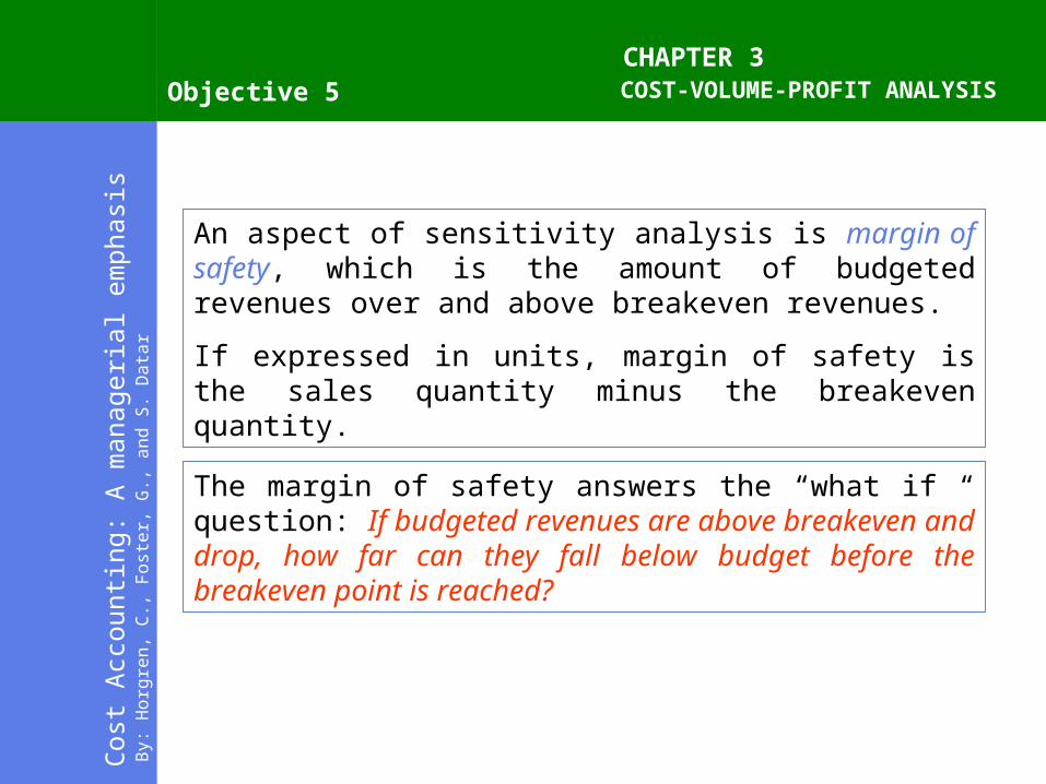
Objective 5
An aspect of sensitivity analysis is margin of safety, which is the amount of budgeted revenues over and above breakeven revenues.
If expressed in units, margin of safety is the sales quantity minus the breakeven quantity.
The margin of safety answers the “what if “ question: If budgeted revenues are above breakeven and drop, how far can they fall below budget before the breakeven point is reached?

COST-VOLUME-PROFIT ANALYSISCHAPTER 3
Cos
t A
ccou
ntin
g: A
man
ager
ial e
mph
asis
By:
Ho
rgre
n,
C.,
Fo
ste
r, G
., a
nd
S.
Da
tar
Objective 5
40 units: budgeted revenues = $8000 ($200*40 units)
Breakeven (25 units): revenues = $5000 ($200*25 units)
Using the given data, for 40 units sold, the margin of safety is $3000 revenues or 15 units if expressed in units
Therefore, margin of safety will be,
$3000 ($8000-$5000) (in terms of revenues)
15 units (40 units – 25 units) (in terms of units)
Back to learning objectives

COST-VOLUME-PROFIT ANALYSISCHAPTER 3
Cos
t A
ccou
ntin
g: A
man
ager
ial e
mph
asis
By:
Ho
rgre
n,
C.,
Fo
ste
r, G
., a
nd
S.
Da
tar
Objective 6
Cost Planning and CVP
Alternative Fixed-Cost/Variable-Cost Structures
CVP-based analysis highlights the risks and returns that an existing cost structure holds for a organization. This insight may lead managers to consider alternative cost structures. CVP analysis can help managers evaluate various alternatives.

COST-VOLUME-PROFIT ANALYSISCHAPTER 3
Cos
t A
ccou
ntin
g: A
man
ager
ial e
mph
asis
By:
Ho
rgre
n,
C.,
Fo
ste
r, G
., a
nd
S.
Da
tar
Objective 6
Scenario:
Consider again our Do-All Software example. Our original example has Mary paying a $2000 booth rental fee. Suppose, however, Computer Conventions offers Mary three rental alternatives:
Option 1: $2000 fixed fee
Option 2: $800 fixed fee plus 15% of convention revenues
Option 3: 25% of convention revenues with no fixed fee
Mary anticipates selling 40 packages. She is interested in how her choice of a rental agreement will affect the income she earns and the risks she faces.

-$3,000.00
-$2,000.00
-$1,000.00
$0.00
$1,000.00
$2,000.00
$3,000.00
$4,000.00
$5,000.00
$6,000.00
$7,000.00
0 10 20 30 40 50 60 70 80 90 100
Units Sold
Op
era
tin
g In
co
me
($
)
Option 1
Option 2
Option 3
Profit-Volume Graph for Alternative Rental Options for Do-All Software
Breakeven point
Breakeven point = 16
Breakeven point = 25
COST-VOLUME-PROFIT ANALYSISCHAPTER 3
Cos
t A
ccou
ntin
g: A
man
ager
ial e
mph
asis
By:
Ho
rgre
n,
C.,
Fo
ste
r, G
., a
nd
S.
Da
tar
Objective 6
Spreadsheets computation

COST-VOLUME-PROFIT ANALYSISCHAPTER 3
Cos
t A
ccou
ntin
g: A
man
ager
ial e
mph
asis
By:
Ho
rgre
n,
C.,
Fo
ste
r, G
., a
nd
S.
Da
tar
Objective 6
If Mary sells 40 packages, each option results in operating income of $1200.
However, if the sales of Mary vary from 40 units, CVP analysis highlights the different risks and returns associated with each option.
margin of safety:
option 1: revenues @ 40 units – revenues @ 25 units = $8000-$5000 = $3000
option 2: revenues @ 40 units – revenues @ 16 units = $8000-$3200 = $4800
option 3: revenues @ 40 units – revenues @ 0 unit = $8000-$0 = $8000
Spreadsheets computation
…the downside risk of option 1 comes from its higher fixed cost and hence higher breakeven point and lower margin of safety.

COST-VOLUME-PROFIT ANALYSISCHAPTER 3
Cos
t A
ccou
ntin
g: A
man
ager
ial e
mph
asis
By:
Ho
rgre
n,
C.,
Fo
ste
r, G
., a
nd
S.
Da
tar
Objective 6
If the units sold drops to 20, what would be the operating income under each option?
…..Option 1 leads to an operating loss of $400 but options 2 and 3 will continue to produce operating income
However, the higher risk in option 1 must be evaluated against its potential benefits
Spreadsheets computation
COST-VOLUME-PROFIT ANALYSISCHAPTER 3
Cos
t A
ccou
ntin
g: A
man
ager
ial e
mph
asis
By:
Ho
rgre
n,
C.,
Fo
ste
r, G
., a
nd
S.
Da
tar
Objective 6
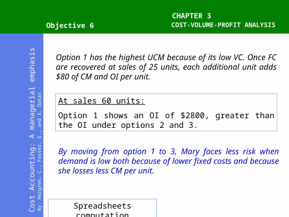
Option 1 has the highest UCM because of its low VC. Once FC are recovered at sales of 25 units, each additional unit adds $80 of CM and OI per unit.
At sales 60 units:
Option 1 shows an OI of $2800, greater than the OI under options 2 and 3.
By moving from option 1 to 3, Mary faces less risk when demand is low both because of lower fixed costs and because she losses less CM per unit.
Spreadsheets computation

COST-VOLUME-PROFIT ANALYSISCHAPTER 3
Cos
t A
ccou
ntin
g: A
man
ager
ial e
mph
asis
By:
Ho
rgre
n,
C.,
Fo
ste
r, G
., a
nd
S.
Da
tar
Objective 6
Operating leverage describes the effects that FC have on changes in OI as changes occur in units sold and hence in CM.
• High FC has high operating leverage
• High operating leverage means small changes in sales will lead to large changes in OI.
sales, OI increases relatively more
sales, OI decline relatively more, leading to a greater risk in losses
Degree of operating leverage equals contribution margin divided by the operating income. ( = CM/OI)
Risk-return trade off measure

COST-VOLUME-PROFIT ANALYSISCHAPTER 3
Cos
t A
ccou
ntin
g: A
man
ager
ial e
mph
asis
By:
Ho
rgre
n,
C.,
Fo
ste
r, G
., a
nd
S.
Da
tar
Objective 6
Degree of operating leverage at sales 40 units
Option 1 Option 2 Option 3
Contribution margin per unit $80 $50 $30
Contribution margin (CM) $3,200 $2,000 $1,200
Operating income (OI) $1,200 $1,200 $1,200
Degree of operating leverage(CM/OI) 2.67 1.67 1.00
A sales increase in 50%
From 40 units to 60 units , CM will increase by 50%, then OI increase will be 50% times the degree of operating leverage.
OI increase would then be,
Option 1: 2.67*50% = 133.5% (from $1200 to $2800)
Option 2: 1.67*50% = 83.5% (from $1200 to $2200)
Option 3: 1.00*50% = 50% (from $1200 to $1800)

COST-VOLUME-PROFIT ANALYSISCHAPTER 3
Cos
t A
ccou
ntin
g: A
man
ager
ial e
mph
asis
By:
Ho
rgre
n,
C.,
Fo
ste
r, G
., a
nd
S.
Da
tar
Objective 6
Effect of Time Horizon
A critical assumption of CVP analysis is that costs can be classified either variable or fixed.
….This classification is affected by the time period being considered for a decision.
….The shorter the time horizon, the higher the percentage of total costs we may view as fixed.
Example

COST-VOLUME-PROFIT ANALYSISCHAPTER 3
Cos
t A
ccou
ntin
g: A
man
ager
ial e
mph
asis
By:
Ho
rgre
n,
C.,
Fo
ste
r, G
., a
nd
S.
Da
tar
Objective 6
Back to learning objectives
Scenario 1:
Suppose a United Airlines plane will depart from its gate in 60 minutes and there are 20 empty seats. A potential passenger arrives bearing a transferable ticket from a competing airline. What are the variable costs to United of placing one more passenger in an otherwise empty seat?
….Variable costs (such as one meal) would be negligible. Virtually, all the costs in this decision situation are fixed.
Scenario 2:
Suppose a United Airlines must decide whether to include another city in its routes.
.....This decision may have a one-year planning horizon. Many more costs would be regarded as variable and fewer as fixed in this decision.

COST-VOLUME-PROFIT ANALYSISCHAPTER 3
Cos
t A
ccou
ntin
g: A
man
ager
ial e
mph
asis
By:
Ho
rgre
n,
C.,
Fo
ste
r, G
., a
nd
S.
Da
tar
Objective 7
Effects of Sales Mix on Income
Sales Mix is the relative combination of quantities of products (or services) that constitutes total unit sales.
If the mix changes, the overall unit sales target may still be achieved. However, the effect on operating income depends on how the original proportions of lower or higher contribution margin products have shifted.

COST-VOLUME-PROFIT ANALYSISCHAPTER 3
Cos
t A
ccou
ntin
g: A
man
ager
ial e
mph
asis
By:
Ho
rgre
n,
C.,
Fo
ste
r, G
., a
nd
S.
Da
tar
Objective 7
Influencing Cost Structures to Manage the Risk-Return Tradeoff
Building up too many fixed costs can be hazardous to a company’s health. Because fixed costs, unlike variable costs, do not automatically decrease as volumes decline, companies with too many fixed costs can lose a considerable amount of money during lean months.
Manager’s decision influence the mix of fixed and variable costs in a company’s cost structure. In making these decisions, managers use forecasts of the effect on net income at different volume levels to evaluate the risk-return tradeoffs involved in various cost structures.

COST-VOLUME-PROFIT ANALYSISCHAPTER 3
Cos
t A
ccou
ntin
g: A
man
ager
ial e
mph
asis
By:
Ho
rgre
n,
C.,
Fo
ste
r, G
., a
nd
S.
Da
tar
Objective 7
Example:
Xerox sells copier machines at lower margins along with maintenance and supplies (for example, paper and toner) contracts a higher margin.
Similarly, Gillette sells razors at low margins and counts on high margins from selling blades. Cellular phone service companies, also, “give away” the cellular phone instrument itself in exchange for higher revenues from using the network.

COST-VOLUME-PROFIT ANALYSISCHAPTER 3
Cos
t A
ccou
ntin
g: A
man
ager
ial e
mph
asis
By:
Ho
rgre
n,
C.,
Fo
ste
r, G
., a
nd
S.
Da
tar
Objective 7
Suppose Mary is now budgeting for the next convention. She plans to sell two software products – Do-All and Superword – and budgets the following:
Do-All Superword Total
Units Sold 60 40 100
Revenues, $200 & $100 per unit $ 12,000 $ 4,000 $ 16,000
Variable costs, $120 & $70 per unit 7,200 2,800 10,000
Unit contribution margin (UCM), $80 and $30 $ 4,800 $ 1,200 6,000
Fixed costs4,500
Operating income$ 1,500

COST-VOLUME-PROFIT ANALYSISCHAPTER 3
Cos
t A
ccou
ntin
g: A
man
ager
ial e
mph
asis
By:
Ho
rgre
n,
C.,
Fo
ste
r, G
., a
nd
S.
Da
tar
Objective 7
What is the breakeven point?
One possible assumption is that the budgeted sales mix (3 units Do-All sold for every 2 units of Superword sold) will not change at different levels of total unit sales.
Let 3Ss = number of units of Do-All to breakevenThen 2S = number of units of Superword to breakeven
Revenues – Variable costs – Fixed costs = Operating income[$200(3S) + $100(2S)] – [$120(3S) + $70(2S)] - $4,500 =0
$300s = $4,500S = 15
No. of units of Do-All to breakeven = 3 x 15 = 45 unitsNo. of units of Superword to breakeven = 2 x 15 = 30 units

COST-VOLUME-PROFIT ANALYSISCHAPTER 3
Cos
t A
ccou
ntin
g: A
man
ager
ial e
mph
asis
By:
Ho
rgre
n,
C.,
Fo
ste
r, G
., a
nd
S.
Da
tar
Objective 7
The breakeven point is 75 units when the sales mix is 45 units of Do-All and 30 units of Superword, which maintains the ratio of 3 units of Do-All for 2 units of Superword.
At this mix, the total contribution margin of $4,500 (Do-All $80 x 45 units = $3,000 + Superword $30 x 30 = $900) equals the fixed costs of $4,500.
Units Sold
Revenues, $200 & $100 per unit
Variable costs, $120 & $70 per unit
Unit contribution margin (UCM), $80 and $30
Fixed costs
Operating income

COST-VOLUME-PROFIT ANALYSISCHAPTER 3
Cos
t A
ccou
ntin
g: A
man
ager
ial e
mph
asis
By:
Ho
rgre
n,
C.,
Fo
ste
r, G
., a
nd
S.
Da
tar
Objective 7
We can also calculate the breakeven point in revenues for the multiple product situation using the weighted-average contribution margin percentage.
Weighted-average contribution margin percentage
Total contribution margin
Total revenues=
=$6,000
$16,000= 0.375 or 37.5%

COST-VOLUME-PROFIT ANALYSISCHAPTER 3
Cos
t A
ccou
ntin
g: A
man
ager
ial e
mph
asis
By:
Ho
rgre
n,
C.,
Fo
ste
r, G
., a
nd
S.
Da
tar
Objective 7
Total revenues required to break even
Fixed costs
Weighted-average contribution margin percentage
=
=$4,500
0.375= $12,000

COST-VOLUME-PROFIT ANALYSISCHAPTER 3
Cos
t A
ccou
ntin
g: A
man
ager
ial e
mph
asis
By:
Ho
rgre
n,
C.,
Fo
ste
r, G
., a
nd
S.
Da
tar
Objective 7
The $16,000 of revenues are in the ratio of 3:1 ($12,000 : $4,000) or 75% :25%. Hence the breakeven revenues of $12,000 should be apportioned in the ratio of 75% ; 25%. This amounts to breakeven revenue dollars of $9,000 (75% x $12,000) of Do-All and $3,000 (25% x $12,000) of Superword. At a selling price of $200 for Do-All and $100 for Superword, this equals 45 units ($9,000 / $200) of Do-All and 30 units ($3,000 / $100) of Superword.
Units Sold
Revenues, $200 & $100 per unit
Variable costs, $120 & $70 per unit
Unit contribution margin (UCM), $80 and $30
Fixed costs
Operating income
COST-VOLUME-PROFIT ANALYSISCHAPTER 3
Cos
t A
ccou
ntin
g: A
man
ager
ial e
mph
asis
By:
Ho
rgre
n,
C.,
Fo
ste
r, G
., a
nd
S.
Da
tar
Objective 7
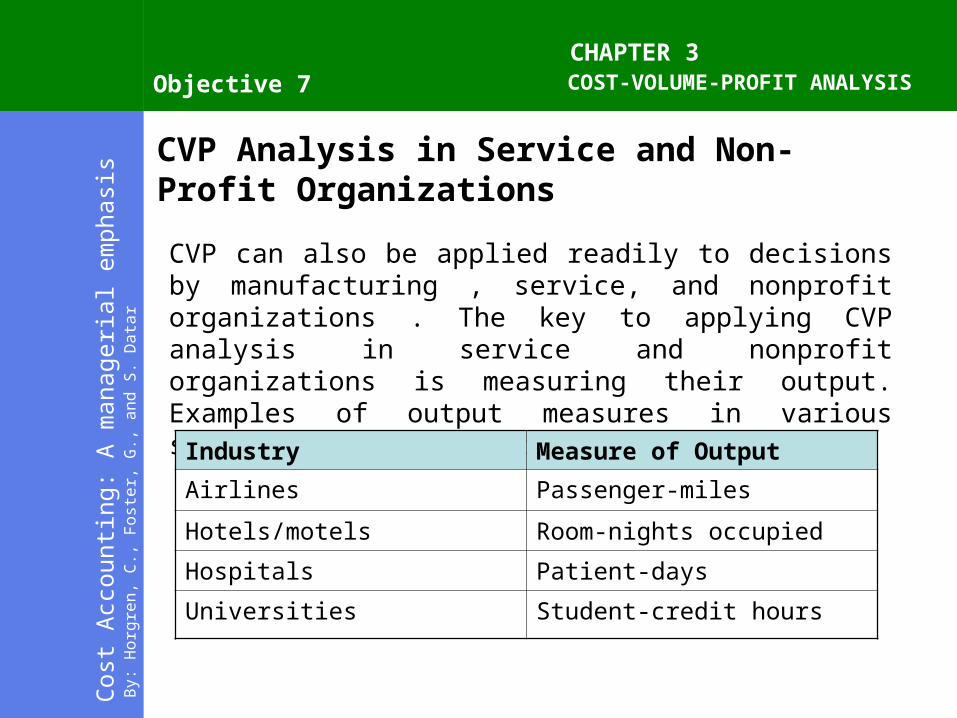
CVP Analysis in Service and Non-Profit Organizations
CVP can also be applied readily to decisions by manufacturing , service, and nonprofit organizations . The key to applying CVP analysis in service and nonprofit organizations is measuring their output. Examples of output measures in various service and nonprofit industries follow.
Industry Measure of Output
Airlines Passenger-miles
Hotels/motels Room-nights occupied
Hospitals Patient-days
Universities Student-credit hours

COST-VOLUME-PROFIT ANALYSISCHAPTER 3
Cos
t A
ccou
ntin
g: A
man
ager
ial e
mph
asis
By:
Ho
rgre
n,
C.,
Fo
ste
r, G
., a
nd
S.
Da
tar
Objective 7
Consider a social welfare agency of the government with a budget appropriation (revenue) for year 2000 of $900,000. This nonprofit agency’s major purpose is to assist handicapped people who are seeking employment. On average, the agency supplements each person’s income by $5,000 annually. The agency’s fixed costs are $270,000. It has no other costs. The agency manager wants to know how many people could be assisted in 2000. We can use CVP analysis here by setting operating income to zero. Let Q be the number handicapped people to be assisted:

COST-VOLUME-PROFIT ANALYSISCHAPTER 3
Cos
t A
ccou
ntin
g: A
man
ager
ial e
mph
asis
By:
Ho
rgre
n,
C.,
Fo
ste
r, G
., a
nd
S.
Da
tar
Objective 7
Revenues – Variable costs – Fixed costs = $0$900,000 - $5,000Q - $270,000 = $0
$5,000Q = $900,000 - $270,000$5,000Q = $630,000
Q = $630,000 / $5,000 per personQ = 126 people

COST-VOLUME-PROFIT ANALYSISCHAPTER 3
Cos
t A
ccou
ntin
g: A
man
ager
ial e
mph
asis
By:
Ho
rgre
n,
C.,
Fo
ste
r, G
., a
nd
S.
Da
tar
Objective 7
Suppose the manager is concerned that the total budget appropriation for 2001 will be reduced by 15% to a new amount of $900,000 x (1 – 0.15) = $765,000. The manager wants to know how many handicapped people could now be assisted. Assume the same amount of monetary assistance per person.
Revenues – Variable costs – Fixed costs = $0$765,000 - $5,000Q - $270,000 = $0
$5,000Q = $765,000 - $270,000$5,000Q = $495,000
Q = $495,000 / $5,000 per personQ = 99 people

COST-VOLUME-PROFIT ANALYSISCHAPTER 3
Cos
t A
ccou
ntin
g: A
man
ager
ial e
mph
asis
By:
Ho
rgre
n,
C.,
Fo
ste
r, G
., a
nd
S.
Da
tar
Objective 7
Note the following two characteristics of the CVP relationships in this nonprofit situation:
1. The percentage drop in service, (126 – 99) / 126, or 21.4%, is more than the 15% reduction in the budget appropriation. Why? Because the existence of $270,000 in fixed costs means that the percentage drop in service exceeds the percentage drop in budget appropriation.
2. If the relationships were graphed, the budget appropriation amount would be a straight horizontal line of $765,000. The manager could adjust operations to stay within this reduced appropriations in one or more three basic ways: (a) Reduce the no. of people assisted, (b) reduce the variable costs (the assistance per person), or (c) reduce the total fixed costs.
Back to learning objectives

COST-VOLUME-PROFIT ANALYSISCHAPTER 3
Cos
t A
ccou
ntin
g: A
man
ager
ial e
mph
asis
By:
Ho
rgre
n,
C.,
Fo
ste
r, G
., a
nd
S.
Da
tar
Objective 8
Multiple Cost Drivers
From the previous topics we have assumed that the number of output units is the only revenue and cost driver. In this section we relax this important assumption and describe how some aspects of CVP analysis can be adapted to the more general case of multiple cost drivers.

COST-VOLUME-PROFIT ANALYSISCHAPTER 3
Cos
t A
ccou
ntin
g: A
man
ager
ial e
mph
asis
By:
Ho
rgre
n,
C.,
Fo
ste
r, G
., a
nd
S.
Da
tar
Objective 8
Let us consider again the single product Do-All Software example. Suppose that Mary Will incur a variable cost of $10 for preparing documents and invoices associated with the sale of Do-All Software. These documents and invoices will need to be prepared for each customer that buys Do-All Software. That is, the cost driver of document-and-invoice-preparation costs is the number of different customers that buy Do-All Software. Mary’s operating income can then be expressed as:
Operating Income
= Revenues - (Costs of each Do-All Software package
X Number of packages sold)
- (Cost of preparing each document and invoice
X Number of documents and invoices)
- Fixed costs
COST-VOLUME-PROFIT ANALYSISCHAPTER 3
Cos
t A
ccou
ntin
g: A
man
ager
ial e
mph
asis
By:
Ho
rgre
n,
C.,
Fo
ste
r, G
., a
nd
S.
Da
tar
Objective 8
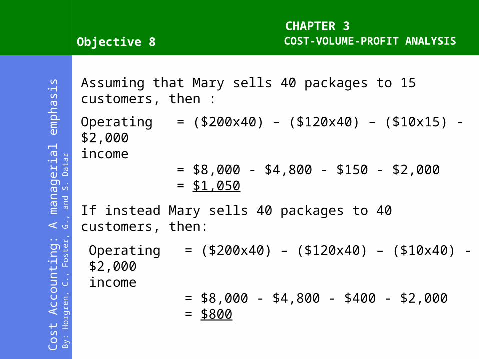
Assuming that Mary sells 40 packages to 15 customers, then :
Operating = ($200x40) – ($120x40) – ($10x15) - $2,000income
= $8,000 - $4,800 - $150 - $2,000= $1,050
If instead Mary sells 40 packages to 40 customers, then:
Operating = ($200x40) – ($120x40) – ($10x40) - $2,000income
= $8,000 - $4,800 - $400 - $2,000= $800

COST-VOLUME-PROFIT ANALYSISCHAPTER 3
Cos
t A
ccou
ntin
g: A
man
ager
ial e
mph
asis
By:
Ho
rgre
n,
C.,
Fo
ste
r, G
., a
nd
S.
Da
tar
Objective 8
Note that the number of packages sold is not the only determinant of Mary’s operating income. For a given number of packages sold, Mary’s operating income will be lower if Mary sells Do-All Software to more customers. Mary’s cost structure depends on two cost drivers – the number of packages sold and the number of customers.
There is no unique breakeven point when there are multiple cost drivers, just as in the case of multiple products.
Back to learning objectives

COST-VOLUME-PROFIT ANALYSISCHAPTER 3
Cos
t A
ccou
ntin
g: A
man
ager
ial e
mph
asis
By:
Ho
rgre
n,
C.,
Fo
ste
r, G
., a
nd
S.
Da
tar
Objective 9
Contribution Margin Versus Gross Margin
Gross Margin = Revenues – Cost of goods sold
Contribution margin = Revenues – All variable costs

COST-VOLUME-PROFIT ANALYSISCHAPTER 3
Cos
t A
ccou
ntin
g: A
man
ager
ial e
mph
asis
By:
Ho
rgre
n,
C.,
Fo
ste
r, G
., a
nd
S.
Da
tar
Objective 9
Merchandising Sector
Contribution margin is computed by deducting all variable costs from revenues, whereas gross margin is computed by deducting only cost of goods sold from revenues.
Contribution Income StatementEmphasizing Contribution Margin
Revenues $ 1,000Variable manufacturing costs $ 120Variable non-manufacturing costs 43 163
Contribution margin 37Fixed manufacturing costsFixed non-manufacturing costs 19Operating income $ 18

COST-VOLUME-PROFIT ANALYSISCHAPTER 3
Cos
t A
ccou
ntin
g: A
man
ager
ial e
mph
asis
By:
Ho
rgre
n,
C.,
Fo
ste
r, G
., a
nd
S.
Da
tar
Objective 9
Merchandising Sector
Contribution margin is computed by deducting all variable costs from revenues, whereas gross margin is computed by deducting only cost of goods sold from revenues.
Financial Accounting Income StatementEmphasizing Gross Margin
Revenues $ 1,000Cost of goods sold 120Gross margin 80
Operating costs ($43 + $19) 62Operating income $ 18

COST-VOLUME-PROFIT ANALYSISCHAPTER 3
Cos
t A
ccou
ntin
g: A
man
ager
ial e
mph
asis
By:
Ho
rgre
n,
C.,
Fo
ste
r, G
., a
nd
S.
Da
tar
Objective 9
Manufacturing Sector
The two areas of difference between contribution margin and gross margin for companies in the manufacturing sector are fixed manufacturing costs and variable non-manufacturing costs.
Contribution Income StatementEmphasizing Contribution Margin
Revenues $ 1,000Variable manufacturing costs $ 250Variable non-manufacturing costs 270 520
Contribution margin 480Fixed manufacturing costs 160Fixed non-manufacturing costs 138 298Operating income $ 182

COST-VOLUME-PROFIT ANALYSISCHAPTER 3
Cos
t A
ccou
ntin
g: A
man
ager
ial e
mph
asis
By:
Ho
rgre
n,
C.,
Fo
ste
r, G
., a
nd
S.
Da
tar
Objective 9
Manufacturing Sector
The two areas of difference between contribution margin and gross margin for companies in the manufacturing sector are fixed manufacturing costs and variable non-manufacturing costs.
Financial Accounting Income StatementEmphasizing Gross Margin
Revenues $ 1,000Cost of goods sold ($250 + $160) 410Gross margin 590 Non-manufacturing costs ($270 + $138) 408Operating income $ 182

COST-VOLUME-PROFIT ANALYSISCHAPTER 3
Cos
t A
ccou
ntin
g: A
man
ager
ial e
mph
asis
By:
Ho
rgre
n,
C.,
Fo
ste
r, G
., a
nd
S.
Da
tar
Objective 9
Fixed manufacturing costs are not deducted from revenues when computing contribution margin but are deducted when computing gross margin. Cost of goods sold in manufacturing company includes all manufacturing costs. Variable non-manufacturing costs are deducted from revenues when computing contribution margin but are not deducted when computing gross margin.

COST-VOLUME-PROFIT ANALYSISCHAPTER 3
Cos
t A
ccou
ntin
g: A
man
ager
ial e
mph
asis
By:
Ho
rgre
n,
C.,
Fo
ste
r, G
., a
nd
S.
Da
tar
End