CVEEN 3310 Lab - Civil & Environmental Engineering at the …bartlett/CVEEN3310/CVEEN 3310 … ·...
60
Steven F. Bartlett, 2010 Lab Notes for CVEEN 3310, Introduction to Geotechnical Engineering Prepared by: Steven F. Bartlett, Ph.D., P.E. Associate Professor Permission for reuse must be sought. Spring Semester 2013 CVEEN 3310 Lab Monday, January 07, 2013 11:43 AM Laboratory Title Page Page 1
Transcript of CVEEN 3310 Lab - Civil & Environmental Engineering at the …bartlett/CVEEN3310/CVEEN 3310 … ·...
Steven F. Bartlett, 2010
Lab Notes for CVEEN 3310, Introduction to Geotechnical Engineering
Prepared by:
Steven F. Bartlett, Ph.D., P.E.Associate Professor
Permission for reuse must be sought.
Spring Semester 2013
CVEEN 3310 LabMonday, January 07, 201311:43 AM
Laboratory Title Page Page 1

© Steven F. Bartlett, 2013
Instructor:
Soil Mechanics Lab – HEDCO 109Phone: 587-7726 FAX: 585-5477E mail: [email protected] (e mail is best).Course website: http://www.civil.utah.edu/~bartlett/CVEEN3310/
Steven F. Bartlett; Office – MCB 2032
Lab Manual: None; Handouts provided by the T.A.
Objectives: (1) To get hands-on experience in performing laboratory and field tests used to measure engineering and index properties of soil; and (2) to understand the use and significance of these properties in practical geotechnical engineering analysis and design.
Grading: The laboratory grade constitutes 20% of the total course grade.
General Policies:
Schedule. Experiments will be performed according to the attached schedule. The schedule may be revised in the event of unforeseen circumstances. You are responsible for reading the laboratory manual and any appropriate handouts prior to the laboratory to determine proper procedures, equipment to be used, etc.
Attendance. ATTENDANCE IS MANDATORY FOR ALL LABORATORY SESSIONS. In the event of an emergency, notify your laboratory teaching assistant as soon as possible that you will be missing the scheduled laboratory session and be prepared to supply evidence to support the nature of your emergency. With approval of the T.A., you may attend another session of the missed lab during that week. If you miss both the laboratory lecture and the laboratory without prior notification, you will receive a zero lab participation grade for that week’s laboratory assignment. No laboratory can be made up.
Tardiness or leaving early should be avoided. If you are tardy, this may result in your group leader giving you deductions in the participation part of your laboratory grade. The laboratory session is scheduled to end at 5:00 p.m. Do not make plans to leave before then because some experiments will require that much time to perform.
Clean-up. Each group is responsible for (a) cleaning the equipment that they used, (b) cleaning up any mess that the group made, and (c) returning the equipment to its proper location. Failure to do so will result in a reduced grade for every student in that group. When you leave the laboratory it should be as clean and organized as when you came.
Pasted from <file:///C:\Users\sfbartlett\Documents\My%20Courses\3310\lab\labsyllabus.doc>
CVEEN 3310 Laboratory General InformationThursday, March 11, 201011:43 AM
Laboratory Information Page 2

© Steven F. Bartlett, 2013
Late Penalty. Laboratory reports are due at the beginning of the laboratory session on the due date. Late laboratory reports will receive a penalty of 10% per day. No lab assignment will be accepted that is more than one week late, unless prior approval has been obtained from the instructor.
Working in Groups and Participation. Students will be required to work in groups. Students in a group must share the responsibility as equally as possible and help each other in performing the necessary tasks to complete the experiments and laboratory report successfully and in professional manner. The laboratory report will be prepared and submitted by the group. Each student's participation grade will be determined by the group leader.
30 percent of your lab grade depends on your in-lab participation.
20 percent of your lab grade depends on your lab calculations and write-up participation
50 percent of your lab grade depends on the score given by the T.A.
Your group leader will hand in a participation sheet that will be used to grade your in-lab and lab write-up participation. They will categorize your participation in the following:
Responsibilities of Group Leader
Organizing group out-of-class activities
Assembling and proof reading laboratory report
Printing and submitting report
Assigning participation grade to team members
Grading of In-lab participation
1) fully participated (30 points), 2) minimal participation, or tardy, or left early (20 points), 3) did not participate (0 points).
Grading of Lab write-up participation
exceeded expectations (25 points: note this includes 5 bonus points), 2) met expectations (20 points), 3) did not met expectations (10 points), 4) did not participate (0 points).
1)
Laboratory format. See course website.
The T.A. will assign students to groups the laboratory session.
Pasted from <file:///C:\Users\sfbartlett\Documents\My%20Courses\3310\lab\labsyllabus.doc>
Laboratory General Info (cont.)Thursday, March 11, 201011:43 AM
Laboratory Information Page 3
© Steven F. Bartlett, 2013
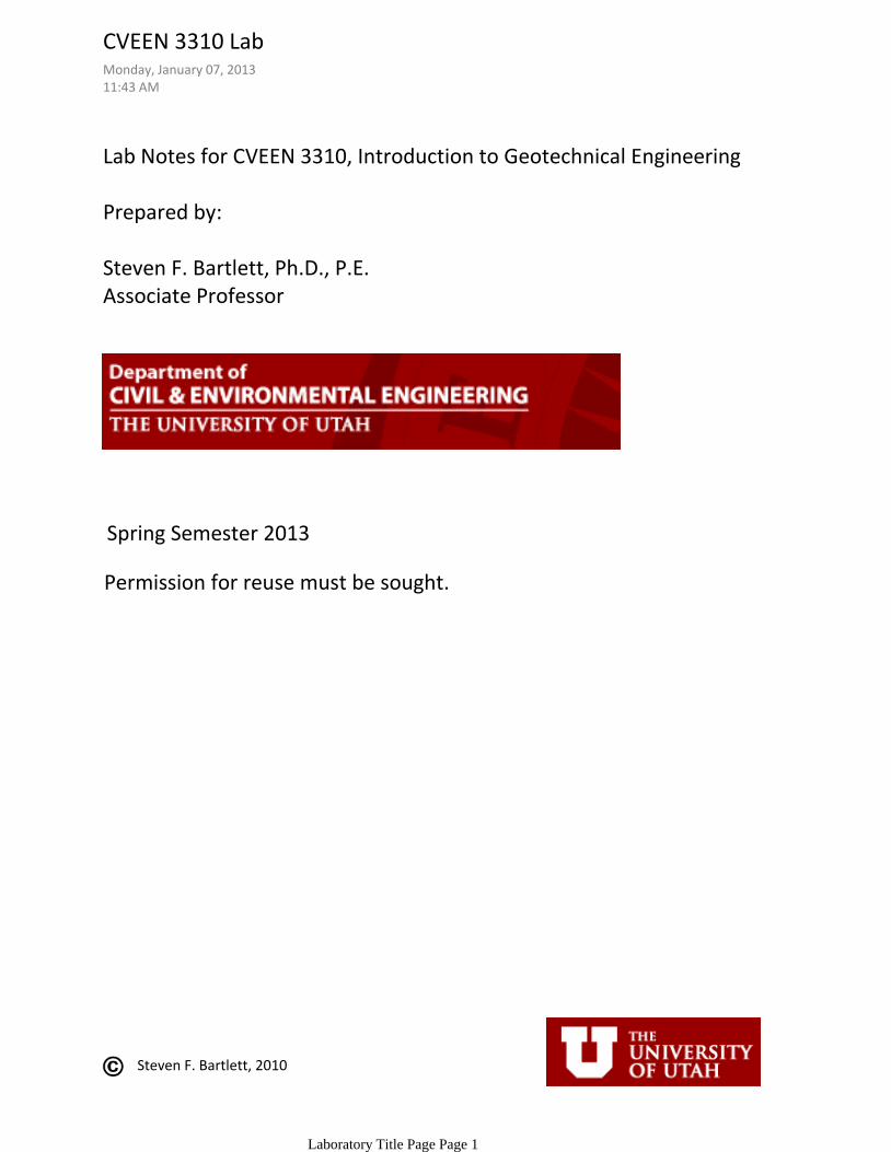
Laboratory Grading SheetThursday, March 11, 201011:43 AM
Laboratory Information Page 4
© Steven F. Bartlett, 2013
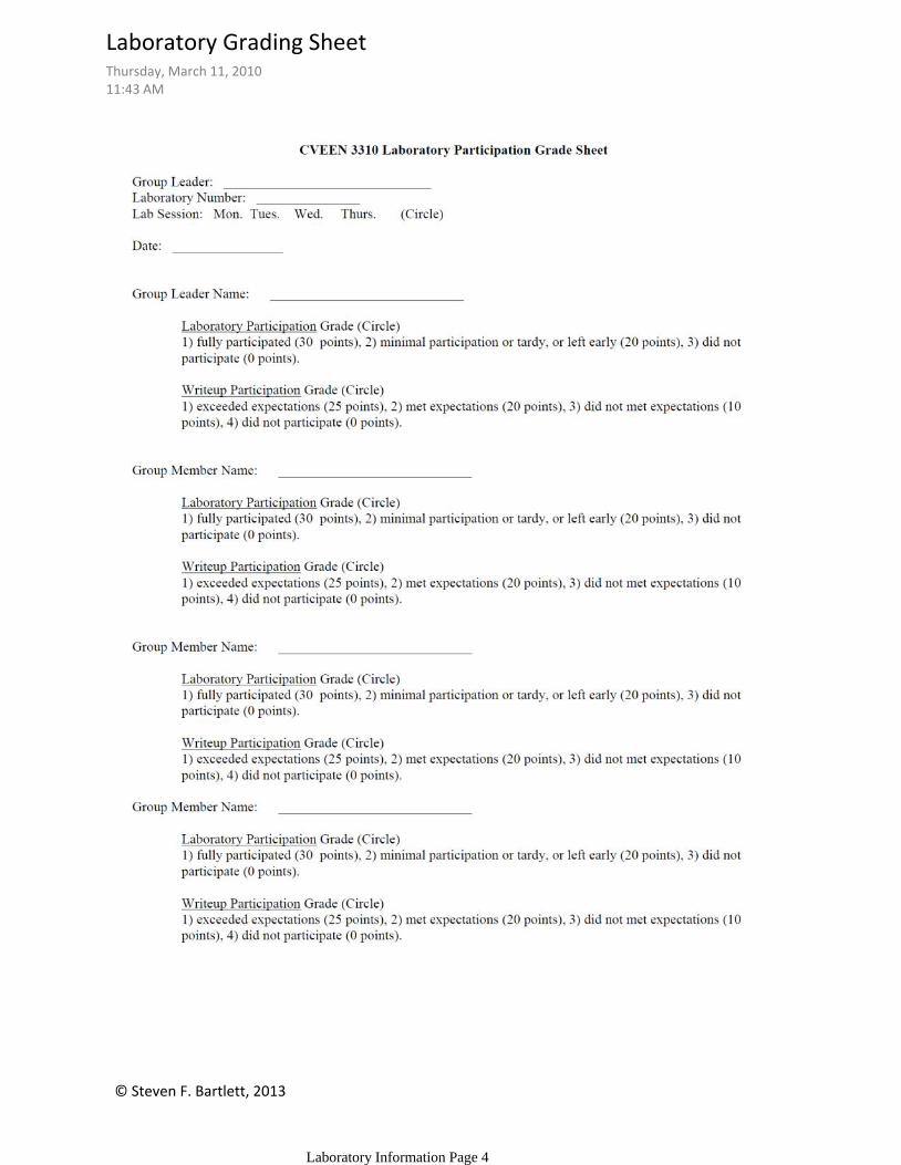
1. The teaching assistant will have the necessary equipment and supplies for each group placed in a designated area. Make note of all equipment and supplies and keep track of everything during the experiment.
2. ABSOLUTELY NO SOIL SHOULD BE PLACED IN THE SINKS. Dump all soil in the appropriate trashcan and wipe off the equipment, dishes, cans, etc. with a paper towel before washing in the sink.
3. TAKE CARE OF THE EQUIPMENT AS IF IT WERE YOUR OWN. Equipment can easily be damaged or broken if proper care is not exercised. Much of the equipment is expensive and difficult to replace or repair. BE ESPECIALLY CAREFUL NOT TO OVERLOAD THE ELECTRONIC SCALES. Check with the T.A. regarding the maximum capacity of the scale you are using. It typically costs $1,000 or more to repair an electronic scale after it has been overloaded.
4. Always note the brand name and model number of the scale you are using on your data sheet. Always use the same scale when weighing materials for the same experiment because there will be slight differences in the calibration of each scale.
5. All equipment and the laboratory must be thoroughly cleaned before leaving. The rule to be followed is that the equipment and the laboratory must be as clean or cleaner than when you started. Each group is responsible for (a) cleaning the equipment that they used, (b) cleaning up any mess that the group made, including the countertops, floor, etc., and (c) returning the equipment to its proper location.
6. When your group is finished with the experiment and all equipment and the laboratory have been cleaned, notify the assistant(s) that you are done. The teaching assistant(s) will check to ensure that all of the equipment is there and is cleaned and will ask your group members to return everything to its proper location. One copy of your laboratory data for that day's experiment should be signed by the group member who recorded the data and turned into the teaching assistant. Your group may leave only after receiving permission from the teaching assistant.
Pasted from <file:///C:\Users\sfbartlett\Documents\My%20Courses\3310\lab\labsyllabus.doc>
Care of Equipment and Clean-upThursday, March 11, 201011:43 AM
Laboratory Information Page 5
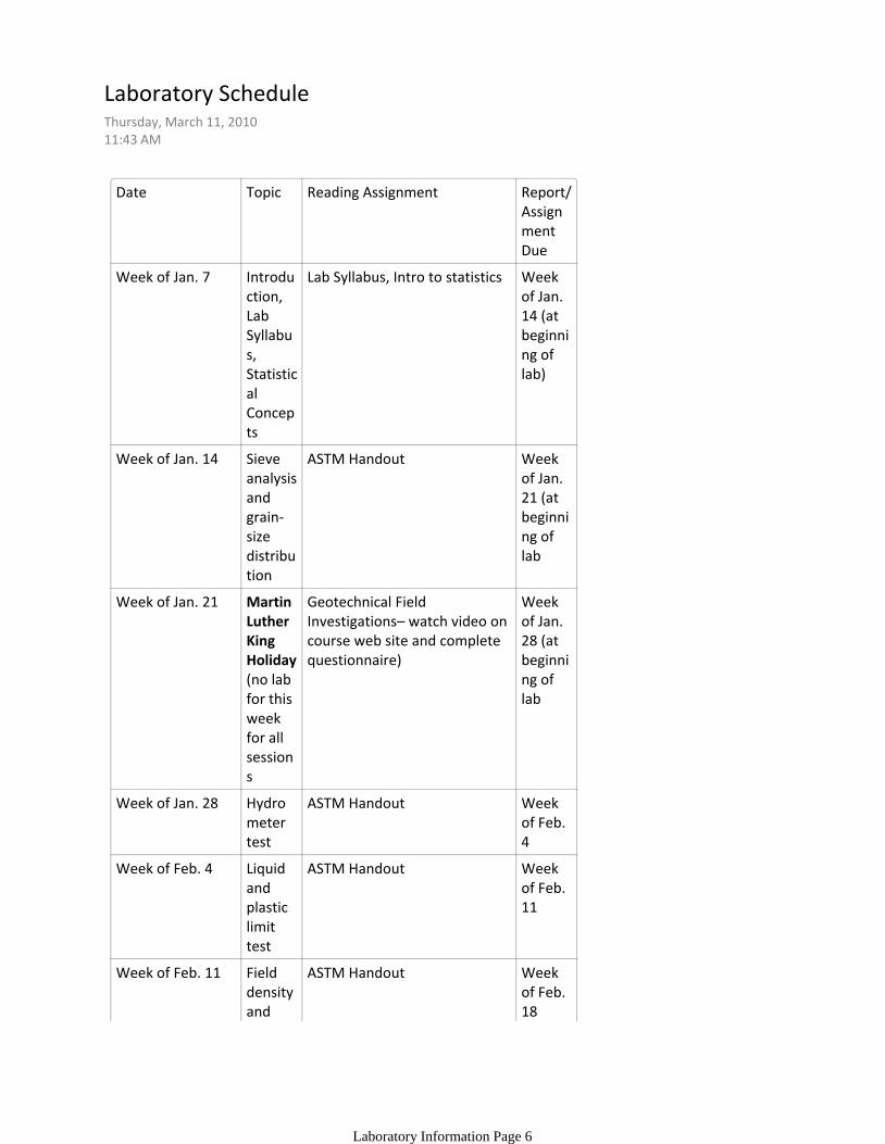
Date Topic Reading Assignment Report/Assignment Due
Week of Jan. 7 Introduction, Lab Syllabus, Statistical Concepts
Lab Syllabus, Intro to statistics Week of Jan. 14 (at beginning of lab)
Week of Jan. 14 Sieve analysis and grain-size distribution
ASTM Handout Week of Jan. 21 (at beginning of lab
Week of Jan. 21 Martin Luther King Holiday (no lab for this week for all sessions
Geotechnical Field Investigations– watch video on course web site and complete questionnaire)
Week of Jan. 28 (at beginning of lab
Week of Jan. 28 Hydrometer test
ASTM Handout Week of Feb. 4
Week of Feb. 4 Liquid and plastic limit test
ASTM Handout Week of Feb. 11
Week of Feb. 11 Field density and sand
ASTM Handout Week of Feb. 18
Laboratory ScheduleThursday, March 11, 201011:43 AM
Laboratory Information Page 6
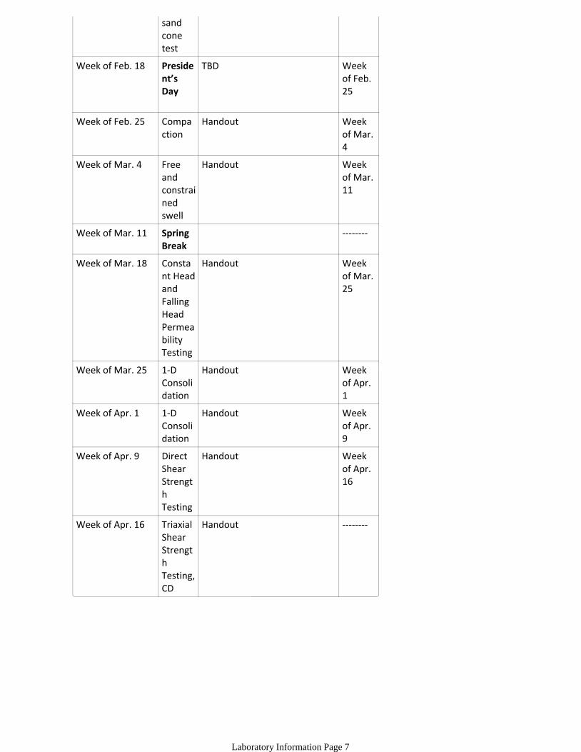
sand cone test
Week of Feb. 18 President’s Day
TBD Week of Feb. 25
Week of Feb. 25 Compaction
Handout Week of Mar. 4
Week of Mar. 4 Free and constrained swell
Handout Week of Mar. 11
Week of Mar. 11 Spring Break
--------
Week of Mar. 18 Constant Head and Falling Head Permeability Testing
Handout Week of Mar. 25
Week of Mar. 25 1-D Consolidation
Handout Week of Apr. 1
Week of Apr. 1 1-D Consolidation
Handout Week of Apr. 9
Week of Apr. 9 Direct Shear Strength Testing
Handout Week of Apr. 16
Week of Apr. 16 Triaxial Shear Strength Testing, CD
Handout --------
Laboratory Information Page 7
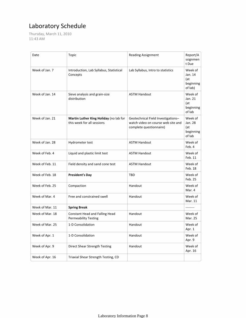
Date Topic Reading Assignment Report/Assignment Due
Week of Jan. 7 Introduction, Lab Syllabus, Statistical Concepts
Lab Syllabus, Intro to statistics Week of Jan. 14 (at beginning of lab)
Week of Jan. 14 Sieve analysis and grain-size distribution
ASTM Handout Week of Jan. 21 (at beginning of lab
Week of Jan. 21 Martin Luther King Holiday (no lab for this week for all sessions
Geotechnical Field Investigations–watch video on course web site and complete questionnaire)
Week of Jan. 28 (at beginning of lab
Week of Jan. 28 Hydrometer test ASTM Handout Week of Feb. 4
Week of Feb. 4 Liquid and plastic limit test ASTM Handout Week of Feb. 11
Week of Feb. 11 Field density and sand cone test ASTM Handout Week of Feb. 18
Week of Feb. 18 President’s Day TBD Week of Feb. 25
Week of Feb. 25 Compaction Handout Week of Mar. 4
Week of Mar. 4 Free and constrained swell Handout Week of Mar. 11
Week of Mar. 11 Spring Break --------
Week of Mar. 18 Constant Head and Falling Head Permeability Testing
Handout Week of Mar. 25
Week of Mar. 25 1-D Consolidation Handout Week of Apr. 1
Week of Apr. 1 1-D Consolidation Handout Week of Apr. 9
Week of Apr. 9 Direct Shear Strength Testing Handout Week of Apr. 16
Week of Apr. 16 Triaxial Shear Strength Testing, CD
Laboratory ScheduleThursday, March 11, 201011:43 AM
Laboratory Information Page 8
© Steven F. Bartlett, 2013
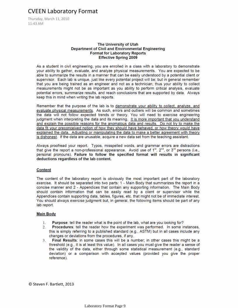
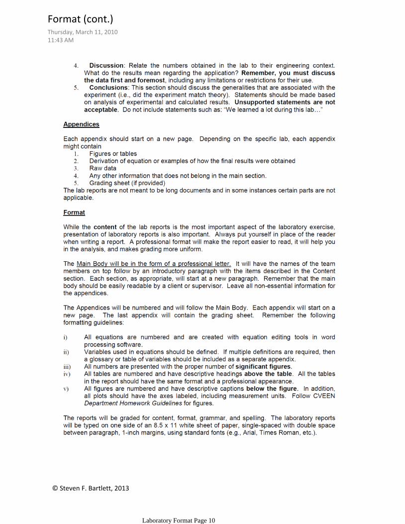
CVEEN Laboratory FormatThursday, March 11, 201011:43 AM
Laboratory Format Page 9
© Steven F. Bartlett, 2013
Format (cont.)Thursday, March 11, 201011:43 AM
Laboratory Format Page 10
© Steven F. Bartlett, 2013
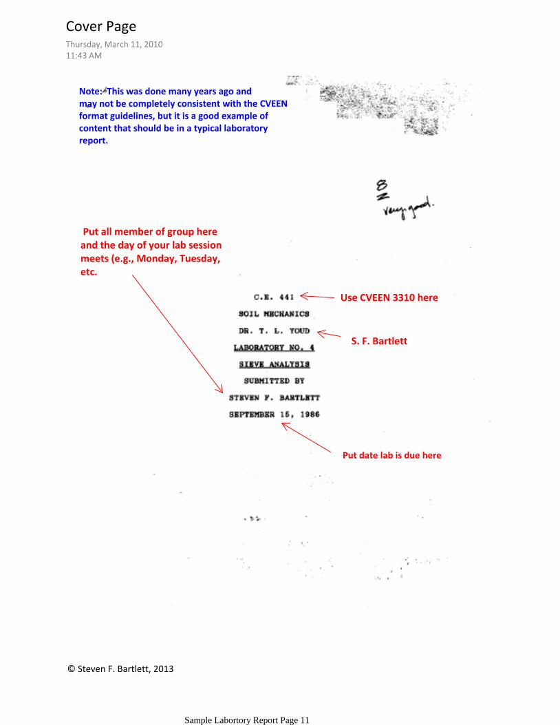
Put all member of group hereand the day of your lab session meets (e.g., Monday, Tuesday, etc.
Use CVEEN 3310 here
Put date lab is due here
S. F. Bartlett
Note: This was done many years ago andmay not be completely consistent with the CVEEN format guidelines, but it is a good example of content that should be in a typical laboratory report.
Cover PageThursday, March 11, 201011:43 AM
Sample Labortory Report Page 11

© Steven F. Bartlett, 2013
Note that you will be using procedures adapted for the course that were modified from published ASTM Standards. In this section, you should state the associated ASTM procedure and include the course procedure as an attachment at the end of the report. Briefly, summarize the procedure. Also describe any significant changes made to the attached procedure and the reason(s). Modifications may be necessary during the lab session due to time limits or other reasons. These need to be discussed.
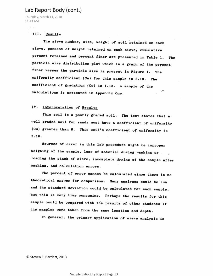
Lab Report BodyThursday, March 11, 201011:43 AM
Sample Labortory Report Page 12
© Steven F. Bartlett, 2013
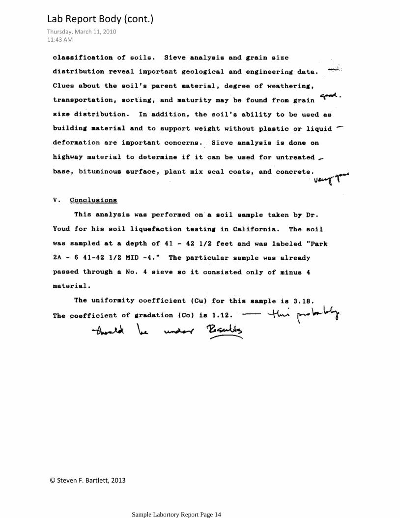
Lab Report Body (cont.)Thursday, March 11, 201011:43 AM
Sample Labortory Report Page 13
© Steven F. Bartlett, 2013
Lab Report Body (cont.)Thursday, March 11, 201011:43 AM
Sample Labortory Report Page 14
© Steven F. Bartlett, 2013
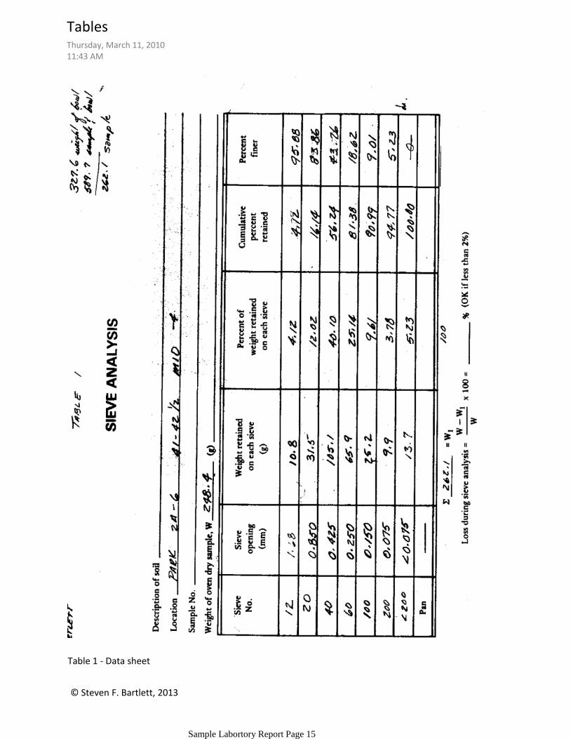
Table 1 - Data sheet
TablesThursday, March 11, 201011:43 AM
Sample Labortory Report Page 15
© Steven F. Bartlett, 2013
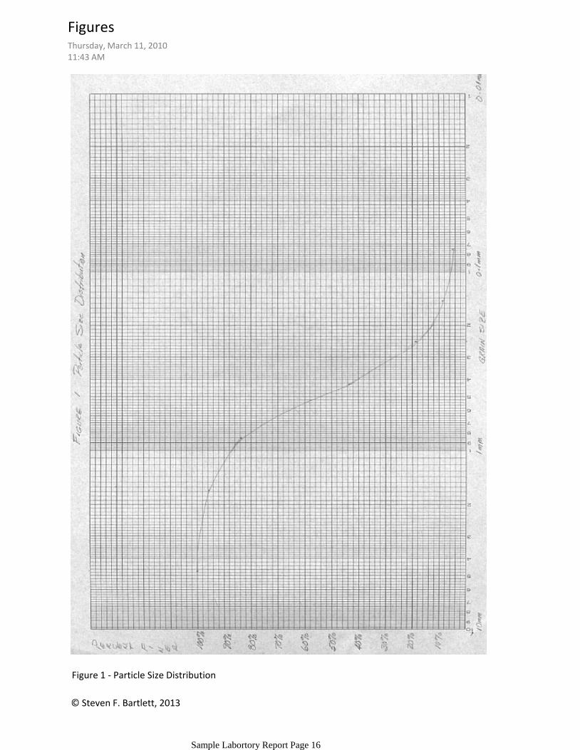
Figure 1 - Particle Size Distribution
FiguresThursday, March 11, 201011:43 AM
Sample Labortory Report Page 16

© Steven F. Bartlett, 2013
Sample CalculationsThursday, March 11, 201011:43 AM
Sample Labortory Report Page 17
© Steven F. Bartlett, 2013
D6913-04(2009) Standard Test Methods for Particle-Size Distribution (Gradation) of Soils Using Sieve Analysis
Reference other sources of information, as appropriate, such as your text book or other sources used in the laboratory session or write-up.
ReferencesThursday, March 11, 201011:43 AM
Sample Labortory Report Page 18

© Steven F. Bartlett, 2013
Attach procedure and other supplemental information○
AttachmentsThursday, March 11, 201011:43 AM
Sample Labortory Report Page 19
Technical Writing HelpsThursday, March 11, 201011:43 AM
Technical Writing Helps Page 20

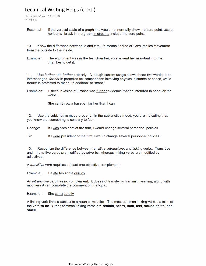
Technical Writing Helps (cont.)Thursday, March 11, 201011:43 AM
Technical Writing Helps Page 21
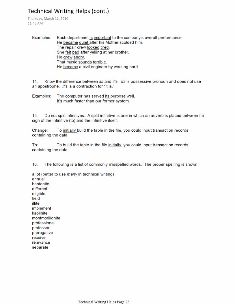
Technical Writing Helps (cont.)Thursday, March 11, 201011:43 AM
Technical Writing Helps Page 22
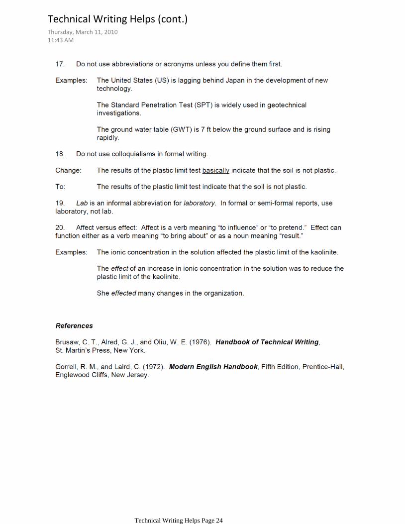
Technical Writing Helps (cont.)Thursday, March 11, 201011:43 AM
Technical Writing Helps Page 23
Technical Writing Helps (cont.)Thursday, March 11, 201011:43 AM
Technical Writing Helps Page 24
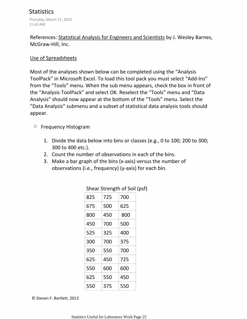
References: Statistical Analysis for Engineers and Scientists by J. Wesley Barnes, McGraw-Hill, Inc.
Use of Spreadsheets
Most of the analyses shown below can be completed using the “Analysis ToolPack” in Microsoft Excel. To load this tool pack you must select “Add-Ins” from the “Tools” menu. When the sub menu appears, check the box in front of the “Analysis ToolPack” and select OK. Reselect the “Tools” menu and “Data Analysis” should now appear at the bottom of the “Tools” menu. Select the “Data Analysis” submenu and a subset of statistical data analysis tools should appear.
Frequency Histogram○
Divide the data below into bins or classes (e.g., 0 to 100; 200 to 300; 300 to 400 etc.).
1.
Count the number of observations in each of the bins.2.Make a bar graph of the bins (x-axis) versus the number of observations (i.e., frequency) (y-axis) for each bin.
3.
Shear Strength of Soil (psf)
825 725 700
675 500 625
800 450 800
450 700 500
525 325 400
300 700 375
350 550 700
625 450 725
550 600 600
625 550 450
550 375 550
© Steven F. Bartlett, 2013
StatisticsThursday, March 11, 201011:43 AM
Statistics Useful for Laboratory Work Page 25
© Steven F. Bartlett, 2013
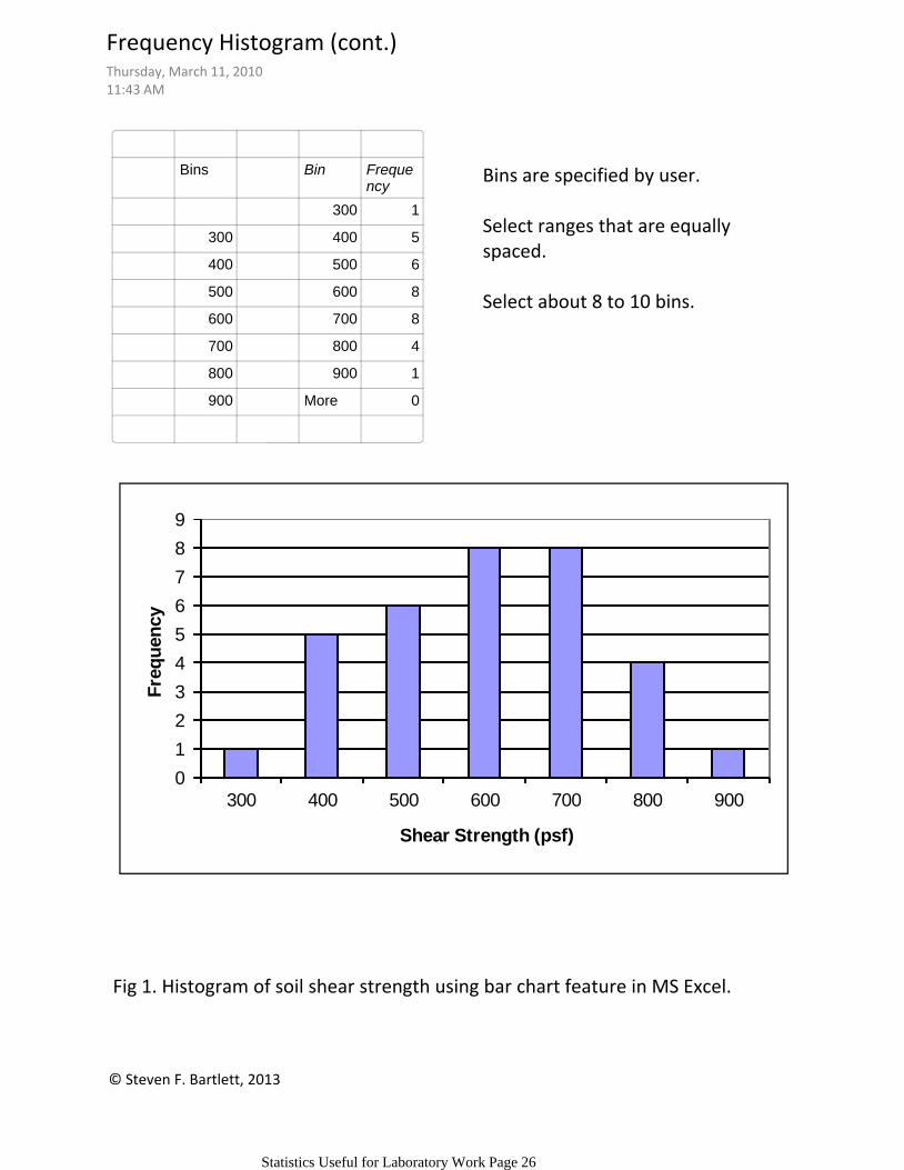
Bins Bin Frequency
300 1
300 400 5
400 500 6
500 600 8
600 700 8
700 800 4
800 900 1
900 More 0
Bins are specified by user.
Select ranges that are equally spaced.
Select about 8 to 10 bins.
0
1
2
3
4
5
6
7
8
9
300 400 500 600 700 800 900
Fre
qu
en
cy
Shear Strength (psf)
Fig 1. Histogram of soil shear strength using bar chart feature in MS Excel.
Frequency Histogram (cont.)Thursday, March 11, 201011:43 AM
Statistics Useful for Laboratory Work Page 26
© Steven F. Bartlett, 2013
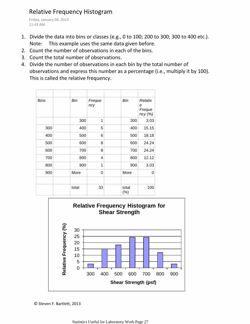
Divide the data into bins or classes (e.g., 0 to 100; 200 to 300; 300 to 400 etc.). Note: This example uses the same data given before.
1.
Count the number of observations in each of the bins.2.Count the total number of observations.3.Divide the number of observations in each bin by the total number of observations and express this number as a percentage (i.e., multiply it by 100). This is called the relative frequency.
4.
Bins Bin Frequency
Bin Relative Frequency (%)
300 1 300 3.03
300 400 5 400 15.15
400 500 6 500 18.18
500 600 8 600 24.24
600 700 8 700 24.24
700 800 4 800 12.12
800 900 1 900 3.03
900 More 0 More 0
total 33 total (%)
100
0
5
10
15
20
25
30
300 400 500 600 700 800 900Re
lati
ve
Fre
qu
en
cy (
%)
Shear Strength (psf)
Relative Frequency Histogram for Shear Strength
Relative Frequency HistogramFriday, January 04, 201311:43 AM
Statistics Useful for Laboratory Work Page 27
© Steven F. Bartlett, 2013
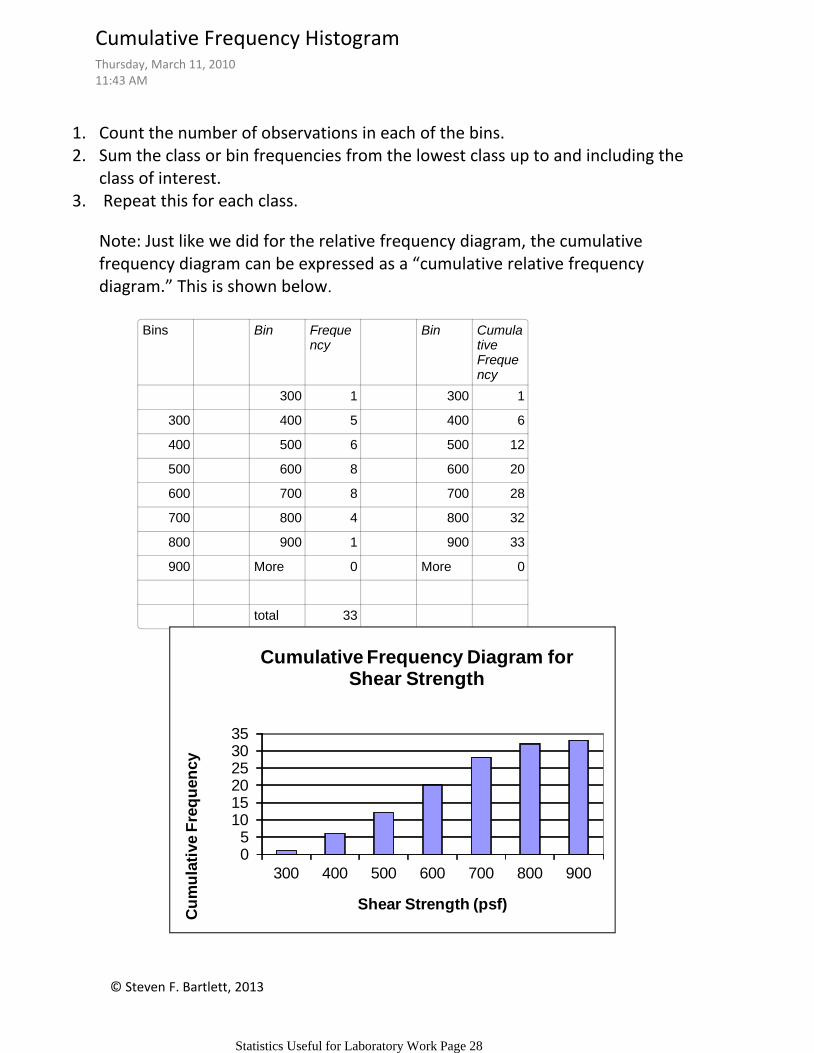
Count the number of observations in each of the bins.1.Sum the class or bin frequencies from the lowest class up to and including the class of interest.
2.
Repeat this for each class.3.
Note: Just like we did for the relative frequency diagram, the cumulative frequency diagram can be expressed as a “cumulative relative frequency diagram.” This is shown below.
Bins Bin Frequency
Bin Cumulative Frequency
300 1 300 1
300 400 5 400 6
400 500 6 500 12
500 600 8 600 20
600 700 8 700 28
700 800 4 800 32
800 900 1 900 33
900 More 0 More 0
total 33
05
101520253035
300 400 500 600 700 800 900
Cu
mu
lati
ve F
req
uen
cy
Shear Strength (psf)
Cumulative Frequency Diagram for Shear Strength
Cumulative Frequency HistogramThursday, March 11, 201011:43 AM
Statistics Useful for Laboratory Work Page 28
© Steven F. Bartlett, 2013
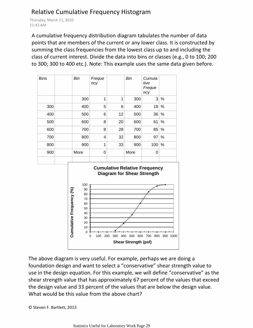
A cumulative frequency distribution diagram tabulates the number of data points that are members of the current or any lower class. It is constructed by summing the class frequencies from the lowest class up to and including the class of current interest. Divide the data into bins or classes (e.g., 0 to 100; 200 to 300; 300 to 400 etc.). Note: This example uses the same data given before.
Bins Bin Frequency
Bin Cumulative Frequency
300 1 1 300 3 %
300 400 5 6 400 18 %
400 500 6 12 500 36 %
500 600 8 20 600 61 %
600 700 8 28 700 85 %
700 800 4 32 800 97 %
800 900 1 33 900 100 %
900 More 0 More 0
0
10
20
30
40
50
60
70
80
90
100
0 100 200 300 400 500 600 700 800 900 1000Cu
mu
lati
ve
Fre
qu
en
cy (
%)
Shear Strength (psf)
Cumulative Relative Frequency Diagram for Shear Strength
The above diagram is very useful. For example, perhaps we are doing a foundation design and want to select a “conservative” shear strength value to use in the design equation. For this example, we will define “conservative” as the shear strength value that has approximately 67 percent of the values that exceed the design value and 33 percent of the values that are below the design value. What would be this value from the above chart?
Relative Cumulative Frequency HistogramThursday, March 11, 201011:43 AM
Statistics Useful for Laboratory Work Page 29
© Steven F. Bartlett, 2013
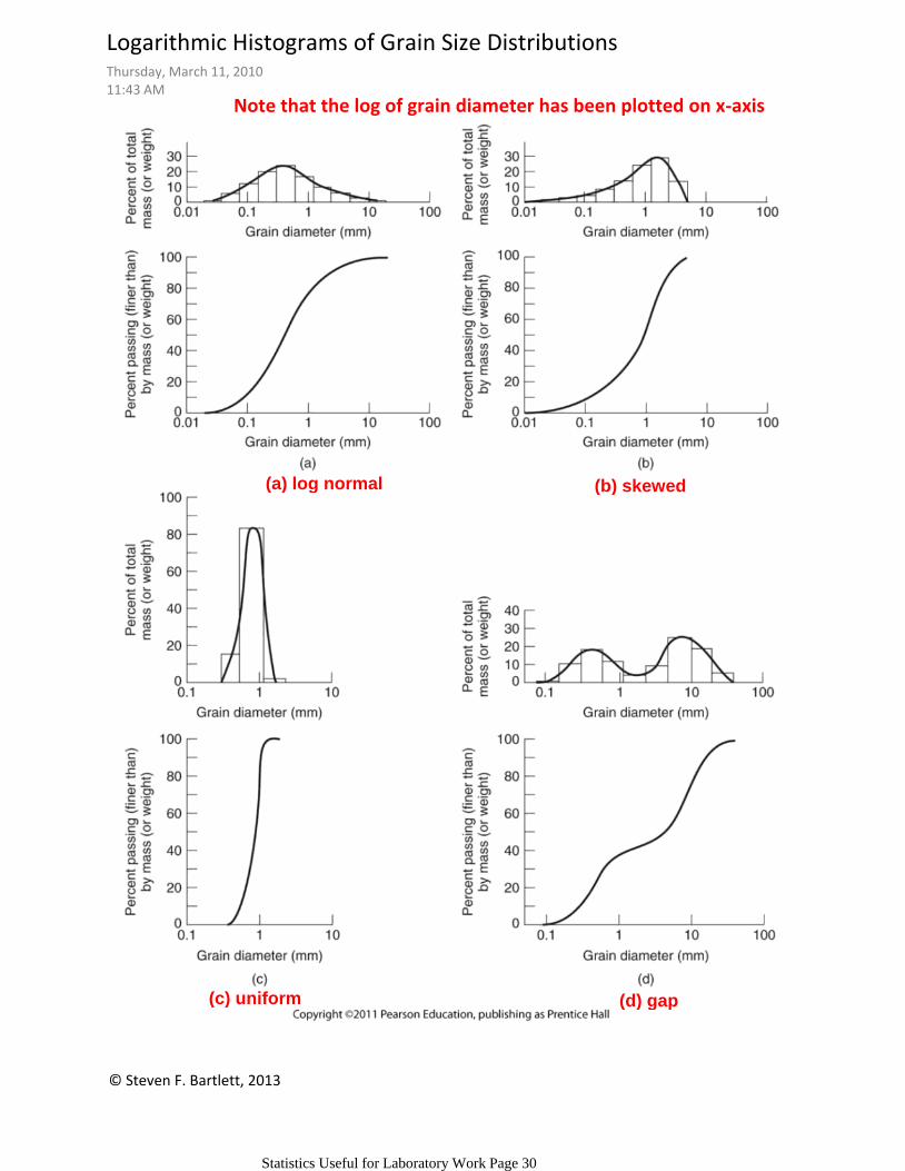
(a) log normal (b) skewed
(c) uniform (d) gap
Note that the log of grain diameter has been plotted on x-axis
Logarithmic Histograms of Grain Size DistributionsThursday, March 11, 201011:43 AM
Statistics Useful for Laboratory Work Page 30
II. Measures of Centrality (Mean, Median, Mode)
_
Sample Mean, xA.
_
x = ( x) / n
The mean is a weighted sum of all possible values, with each value receiving the same weight. It is calculated from:
where Σ x is sum of the all the observations and n is the number of observations (i.e., sample size).
What is the mean for the shear strength data?
MedianB.
The median is the value that exactly divides the cumulative frequency distribution into two equal halves.
What is the median for the shear strength data given in IA?
ModeC.
The mode is any local maximum of the frequency or relative frequency diagram. Thus, it is possible for a sample to have more than one mode.
What is the mode for the shear strength data?
© Steven F. Bartlett, 2013
Descriptive StatisticsThursday, March 11, 201011:43 AM
Statistics Useful for Laboratory Work Page 31

© Steven F. Bartlett, 2013
III. Measures of Variation (Dispersion) about the Mean
Sample variance, s2A.
Although histograms and frequency tables are a simple way of showing variations within a data set, it is often more useful to describe the sample variation using the sample variance. This statistic is a measure of the dispersion about the mean.
_
_ _
s2 = (S (xi - x)2 ) /( n - 1)
The sample variance is calculated from:
where: s2 = variance, (xi - x)2 is summed for i = 1 to i = n, and x is the sample mean.
What is the sample variance for the shear strength data?
Sample standard deviation, sB.
The sample standard deviation is familiar to most people and is simply the square root of the sample variance.
s = (s2)1/2
What is the standard deviation of the shear strength data?
Sample coefficient of variation, cvC.
_cv (%) = (s / x) 100
Another widely used statistic is the coefficient of variation. This statistic gives a rough measure of the relative variation by expressing the ratio of s as a percentage of the sample mean.
What is the coefficient of variation for the shear strength data?
Descriptive Statistics (cont.)Thursday, March 11, 201011:43 AM
Statistics Useful for Laboratory Work Page 32
© Steven F. Bartlett, 2013
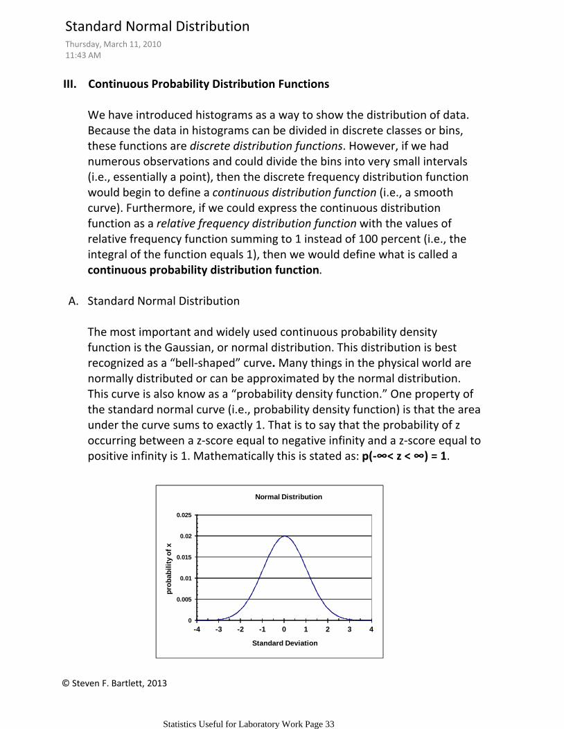
III. Continuous Probability Distribution Functions
We have introduced histograms as a way to show the distribution of data. Because the data in histograms can be divided in discrete classes or bins, these functions are discrete distribution functions. However, if we had numerous observations and could divide the bins into very small intervals (i.e., essentially a point), then the discrete frequency distribution function would begin to define a continuous distribution function (i.e., a smooth curve). Furthermore, if we could express the continuous distribution function as a relative frequency distribution function with the values of relative frequency function summing to 1 instead of 100 percent (i.e., the integral of the function equals 1), then we would define what is called a continuous probability distribution function.
Standard Normal DistributionA.
The most important and widely used continuous probability density function is the Gaussian, or normal distribution. This distribution is best recognized as a “bell-shaped” curve. Many things in the physical world are normally distributed or can be approximated by the normal distribution. This curve is also know as a “probability density function.” One property of the standard normal curve (i.e., probability density function) is that the area under the curve sums to exactly 1. That is to say that the probability of z occurring between a z-score equal to negative infinity and a z-score equal to positive infinity is 1. Mathematically this is stated as: p(-∞< z < ∞) = 1.
0
0.005
0.01
0.015
0.02
0.025
-4 -3 -2 -1 0 1 2 3 4
pro
bab
ilit
y o
f x
Standard Deviation
Normal Distribution
Standard Normal DistributionThursday, March 11, 201011:43 AM
Statistics Useful for Laboratory Work Page 33
© Steven F. Bartlett, 2013
Note that for the standard normal distribution the x-axis is plotted in terms of standard deviations or z-score and the y-axis is the probability of that z-score.
_
_z = ( x - x ) / s
The z-score is calculated from:
where x = value of interest, x is the sample mean (which is an estimate of the population mean) and s is the sample standard deviation (which is an estimate of the population standard deviation).
Note also that if x is equal to the sample mean, then z equals zero. A z-score of 1 means that the value of interest is located exactly 1 standard deviation above the mean. A z-score of -1 means that the value of interest is exactly 1 standard deviation below the mean.
If data are normally distributed then approximately 67 percent or two-thirds of the data are found between ± 1 standard deviation (-1 < z < 1) and 95 percent of the data are found between ± 2 standard deviations (-2 < z < 2).
What is the z-score for a shear strength value of 400 psf using the shear strength data to estimate the mean and standard deviation? How many standard deviations above or below the mean is a value of 400 psf?
Standard Normal Distribution and z-scoreThursday, March 11, 201011:43 AM
Statistics Useful for Laboratory Work Page 34

© Steven F. Bartlett, 2013
Cumulative Normal DistributionB.
Recall that we can form a cumulative relative frequency diagram from a relative frequency diagram. Likewise, we can form a cumulative normal distribution from the standard normal distribution by simply integrating the standard normal curve. The y-axis of the cumulative normal distribution curve gives the probability z is less than or equal to corresponding z-score on the x-axis.
0
0.1
0.2
0.3
0.4
0.5
0.6
0.7
0.8
0.9
1
-4 -3 -2 -1 0 1 2 3 4
pro
bab
ilit
y o
f z <
z*
z-score
Cumulative Normal Distribution
Example: The shear strength of a soil layer is normally distributed with a mean of 100 kPa and a standard deviation of 5 kPa. What is the probability that the strength of one sample taken from this layer is less than 93 kPa?
z* = (93 - 100) / 5 = -1.4p(z < z*) = ?p( z < -1.4) = 0.080757
thus,
p(x < 93 kPa) = 8.0757 percent
Cumulative Normal DistributionThursday, March 11, 201011:43 AM
Statistics Useful for Laboratory Work Page 35
© Steven F. Bartlett, 2013
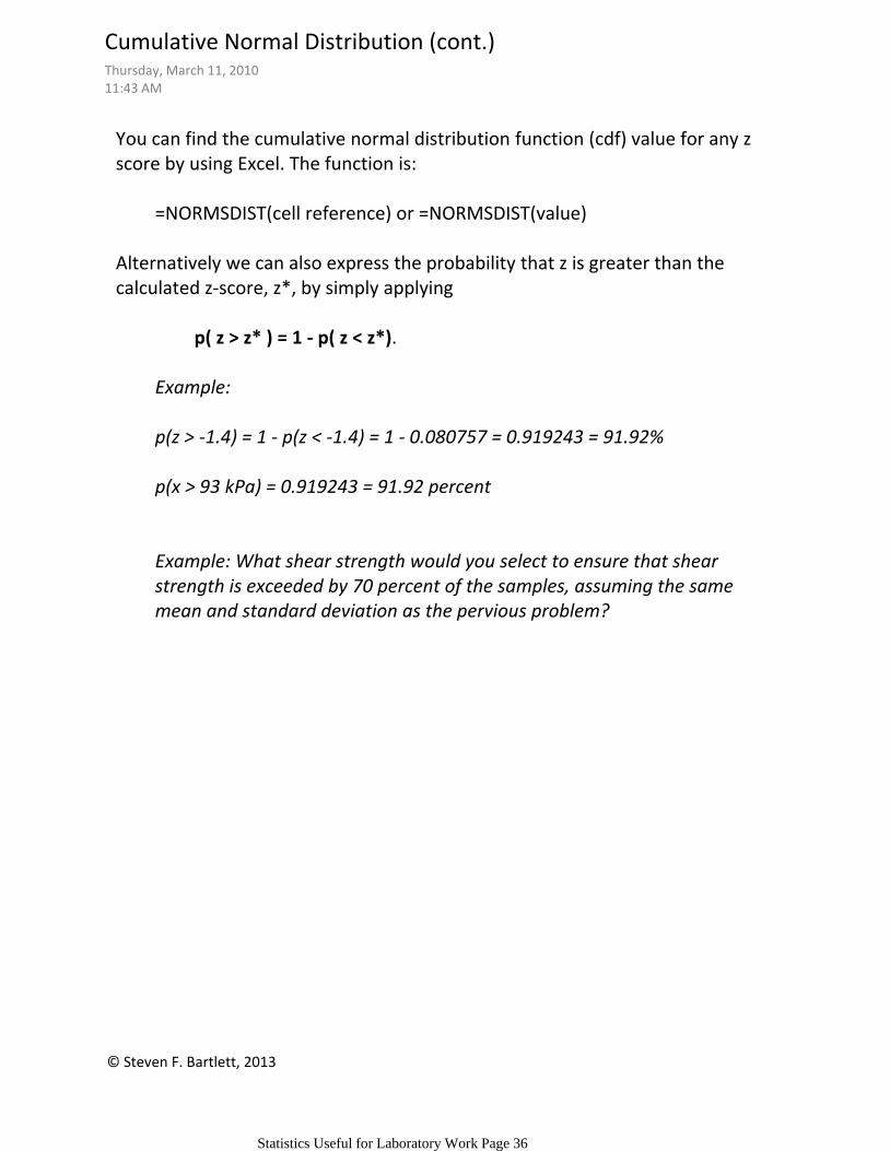
You can find the cumulative normal distribution function (cdf) value for any z score by using Excel. The function is:
=NORMSDIST(cell reference) or =NORMSDIST(value)
Alternatively we can also express the probability that z is greater than the calculated z-score, z*, by simply applying
p( z > z* ) = 1 - p( z < z*).
Example:
p(z > -1.4) = 1 - p(z < -1.4) = 1 - 0.080757 = 0.919243 = 91.92%
p(x > 93 kPa) = 0.919243 = 91.92 percent
Example: What shear strength would you select to ensure that shear strength is exceeded by 70 percent of the samples, assuming the same mean and standard deviation as the pervious problem?
Cumulative Normal Distribution (cont.)Thursday, March 11, 201011:43 AM
Statistics Useful for Laboratory Work Page 36

© Steven F. Bartlett, 2013
In statistics, simple linear regression is the least squares estimator of a linear regression model with a single explanatory variable. In other words, simple linear regression fits a straight line through the set of n points in such a way that makes the sum of squared residuals of the model (that is, vertical distances between the points of the data set and the fitted line) as small as possible.The adjective simple refers to the fact that this regression is one of the simplest in statistics. The slope of the fitted line is equal to the correlation between y and xcorrected by the ratio of standard deviations of these variables. The intercept of the fitted line is such that it passes through the center of mass (x, y) of the data points.
Other regression methods besides the simple ordinary least squares (OLS) also exist (see linear regression model). In particular, when one wants to do regression by eye, people usually tend to draw a slightly steeper line, closer to the one produced by the total least squares method. This occurs because it is more natural for one's mind to consider the orthogonal distances from the observations to the regression line, rather than the vertical ones as OLS method does
Pasted from <http://en.wikipedia.org/wiki/Simple_linear_regression>
Data showing a linear trend or correlation between x and y
Linear RegressionThursday, March 11, 201011:43 AM
Statistics Useful for Laboratory Work Page 37
© Steven F. Bartlett, 2013
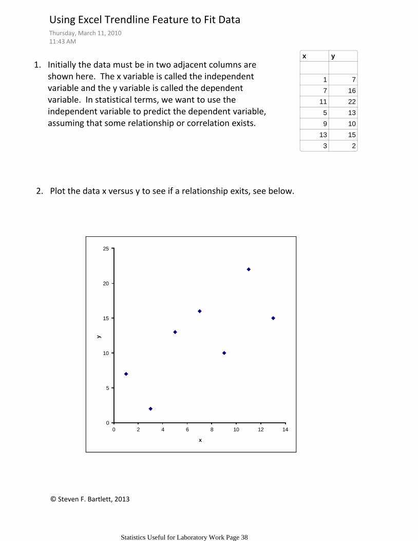
x y
1 7
7 16
11 22
5 13
9 10
13 15
3 2
Initially the data must be in two adjacent columns are shown here. The x variable is called the independent variable and the y variable is called the dependent variable. In statistical terms, we want to use the independent variable to predict the dependent variable, assuming that some relationship or correlation exists.
1.
Plot the data x versus y to see if a relationship exits, see below.2.
0
5
10
15
20
25
0 2 4 6 8 10 12 14
y
x
Using Excel Trendline Feature to Fit DataThursday, March 11, 201011:43 AM
Statistics Useful for Laboratory Work Page 38
© Steven F. Bartlett, 2013
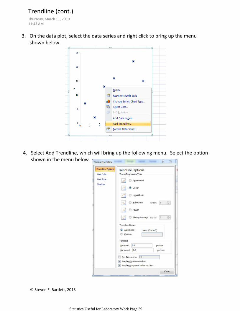
On the data plot, select the data series and right click to bring up the menu shown below.
3.
Select Add Trendline, which will bring up the following menu. Select the option shown in the menu below.
4.
Trendline (cont.)Thursday, March 11, 201011:43 AM
Statistics Useful for Laboratory Work Page 39
© Steven F. Bartlett, 2013
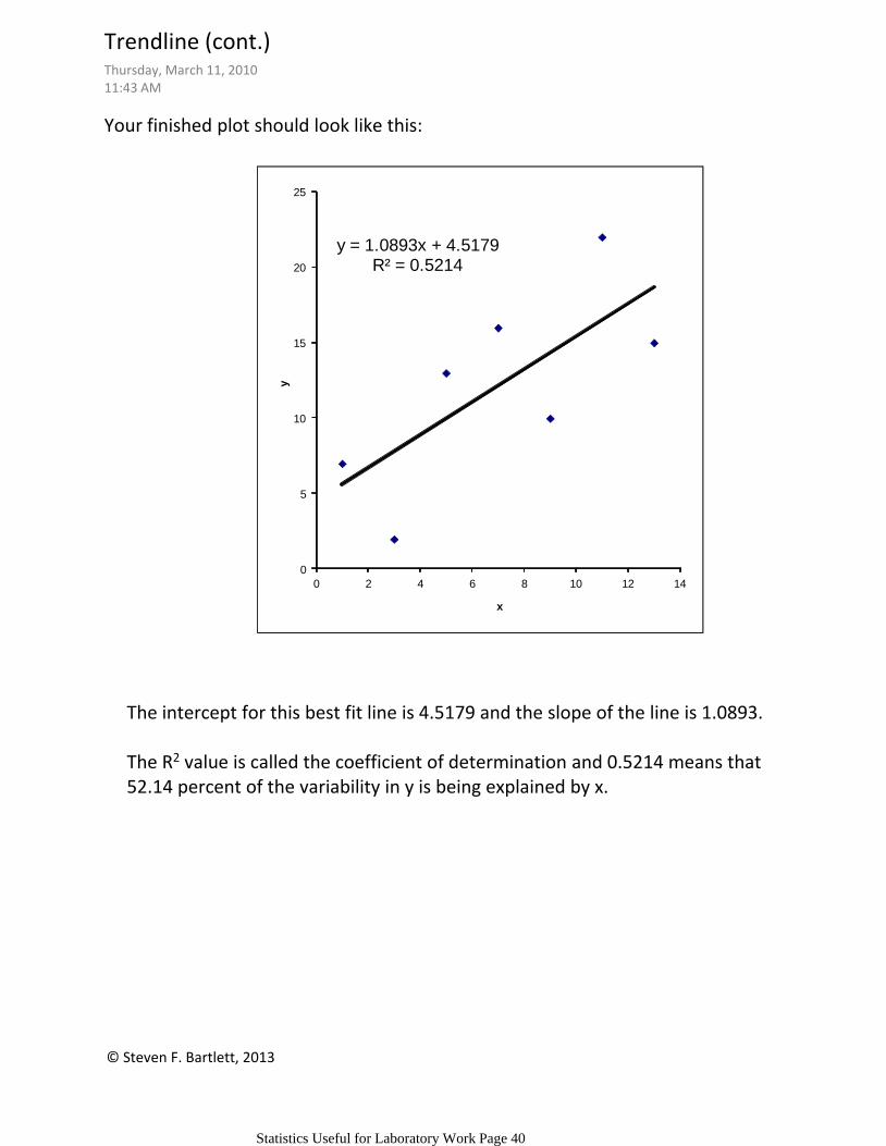
Your finished plot should look like this:
y = 1.0893x + 4.5179R² = 0.5214
0
5
10
15
20
25
0 2 4 6 8 10 12 14
y
x
The intercept for this best fit line is 4.5179 and the slope of the line is 1.0893.
The R2 value is called the coefficient of determination and 0.5214 means that 52.14 percent of the variability in y is being explained by x.
Trendline (cont.)Thursday, March 11, 201011:43 AM
Statistics Useful for Laboratory Work Page 40
© Steven F. Bartlett, 2013
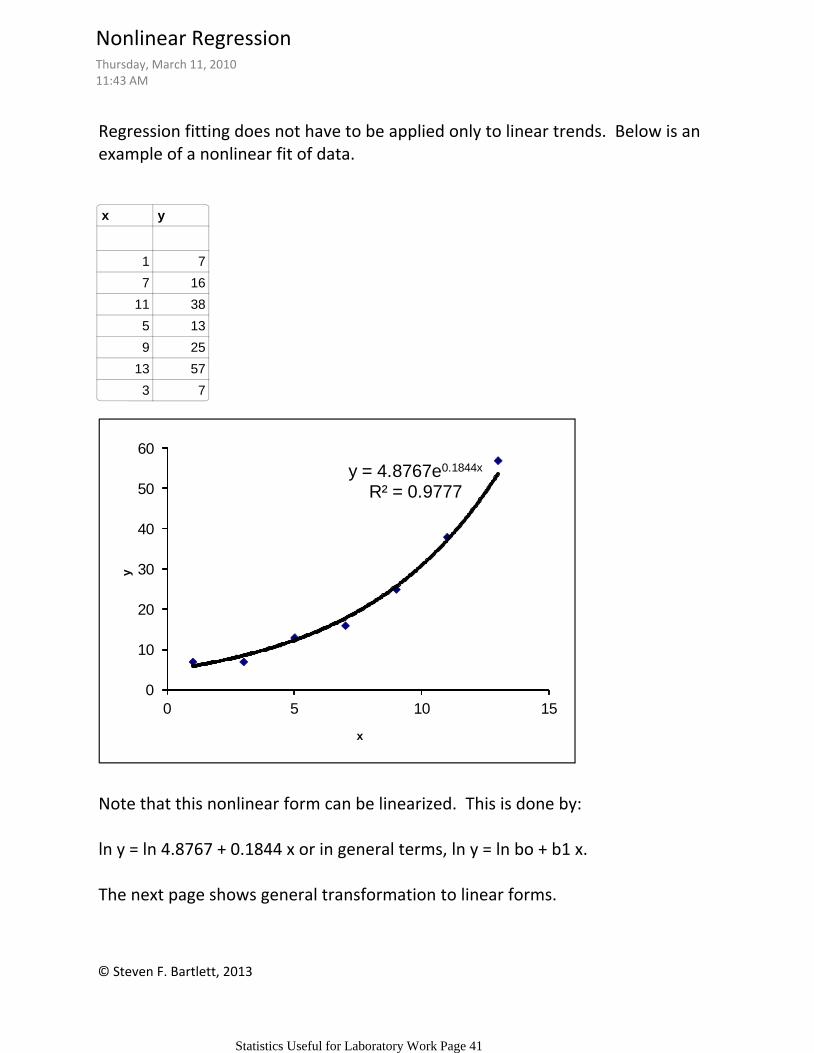
Regression fitting does not have to be applied only to linear trends. Below is an example of a nonlinear fit of data.
x y
1 7
7 16
11 38
5 13
9 25
13 57
3 7
y = 4.8767e0.1844x
R² = 0.9777
0
10
20
30
40
50
60
0 5 10 15
y
x
Note that this nonlinear form can be linearized. This is done by:
ln y = ln 4.8767 + 0.1844 x or in general terms, ln y = ln bo + b1 x.
The next page shows general transformation to linear forms.
Nonlinear RegressionThursday, March 11, 201011:43 AM
Statistics Useful for Laboratory Work Page 41
© Steven F. Bartlett, 2013
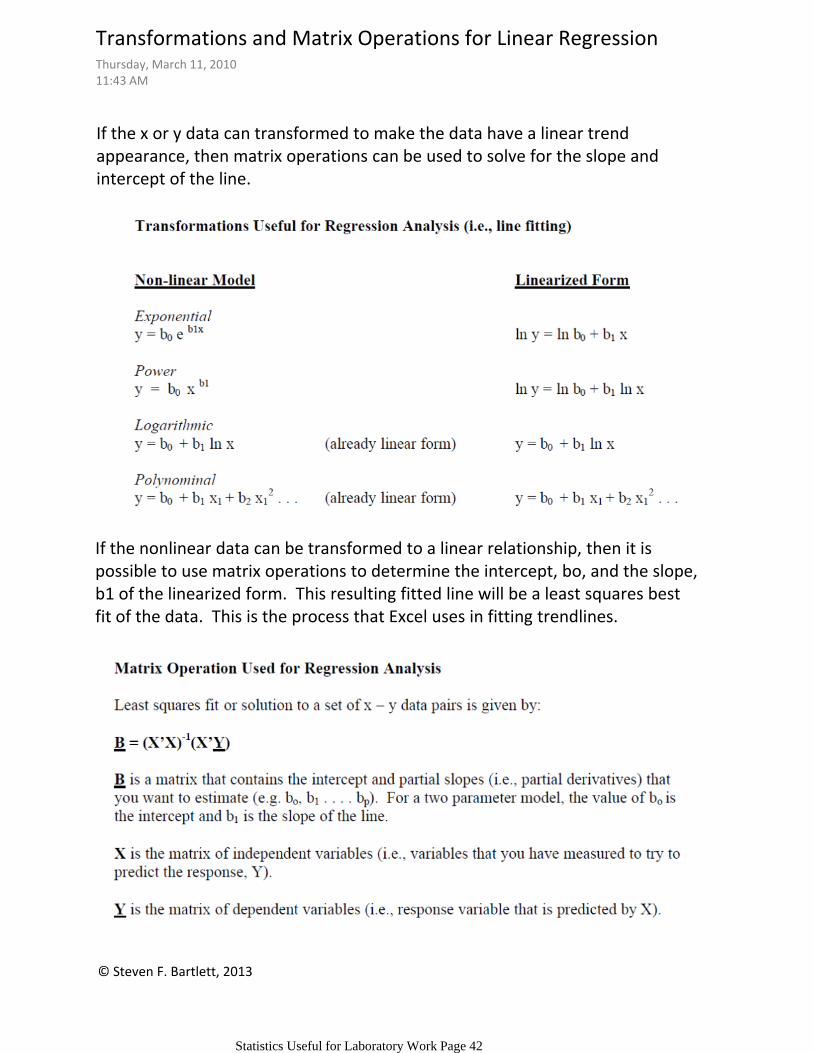
If the x or y data can transformed to make the data have a linear trend appearance, then matrix operations can be used to solve for the slope and intercept of the line.
If the nonlinear data can be transformed to a linear relationship, then it is possible to use matrix operations to determine the intercept, bo, and the slope, b1 of the linearized form. This resulting fitted line will be a least squares best fit of the data. This is the process that Excel uses in fitting trendlines.
Transformations and Matrix Operations for Linear RegressionThursday, March 11, 201011:43 AM
Statistics Useful for Laboratory Work Page 42
© Steven F. Bartlett, 2013
Transformations and Matrix Operations (cont.)Thursday, March 11, 201011:43 AM
Statistics Useful for Laboratory Work Page 43
© Steven F. Bartlett, 2013
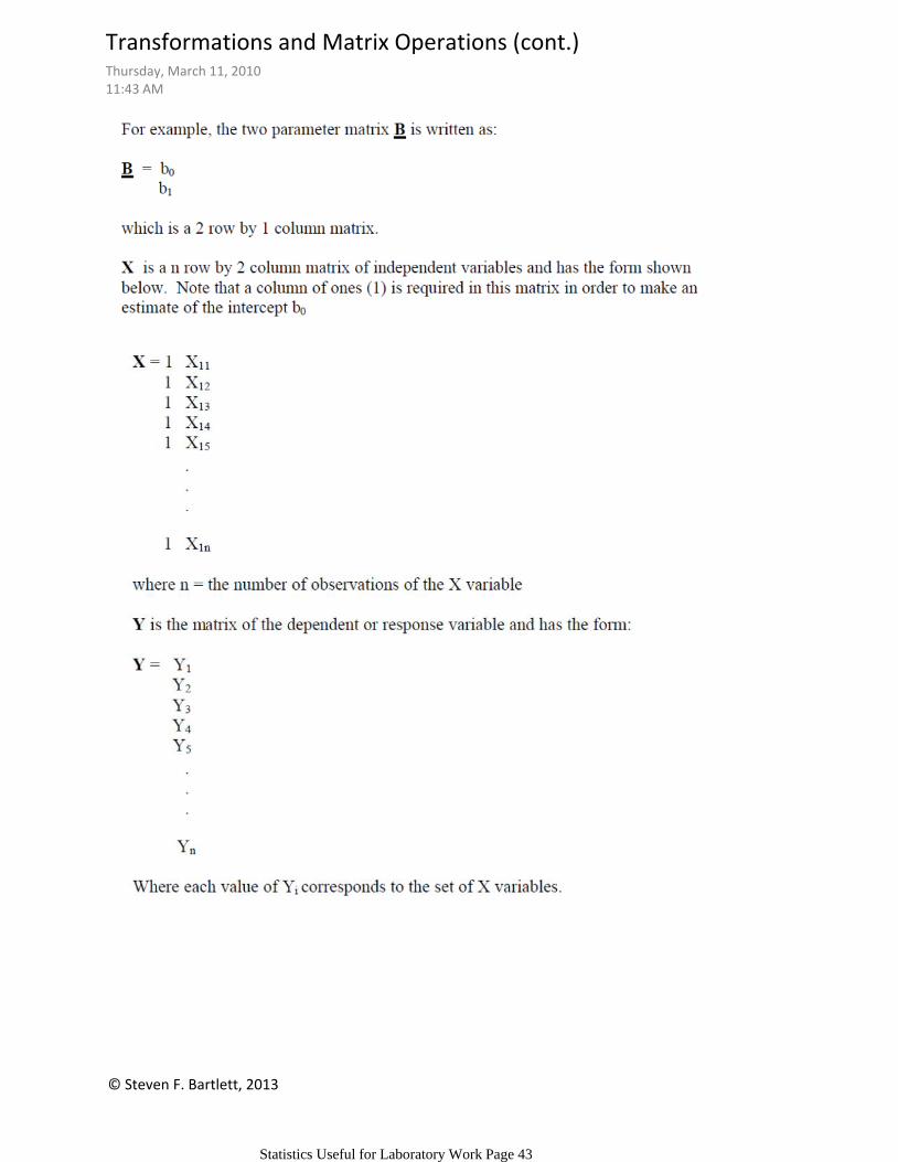
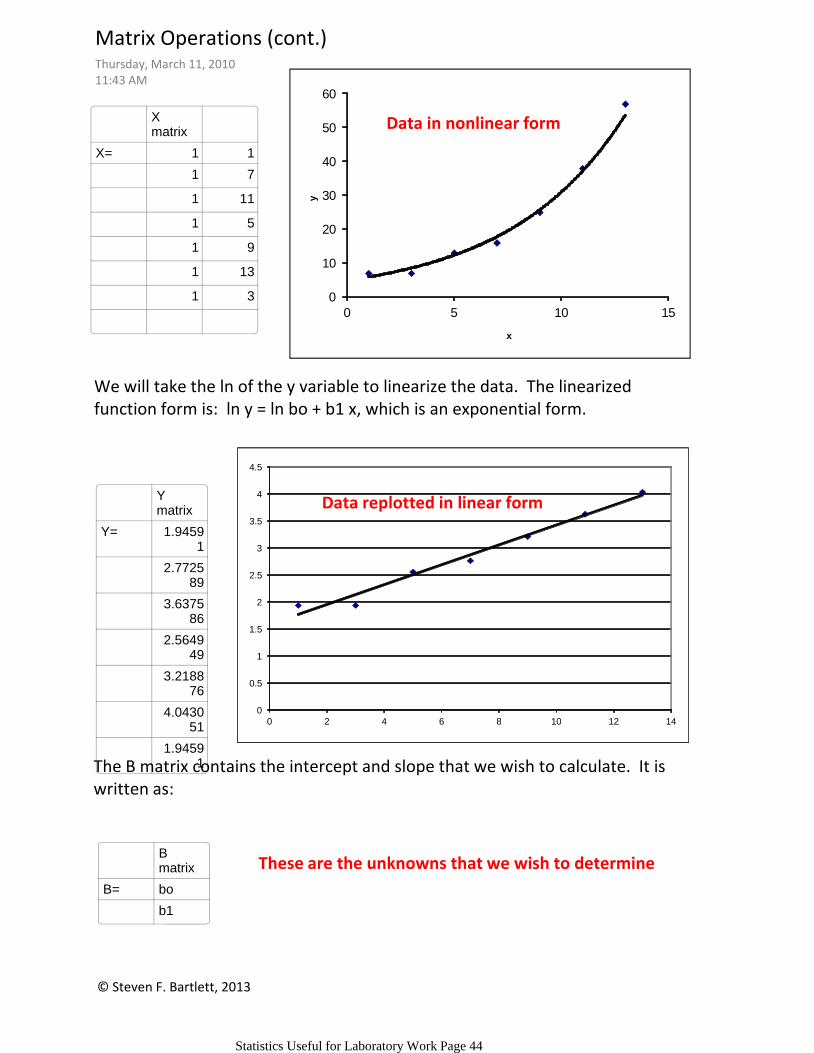
X matrix
X= 1 1
1 7
1 11
1 5
1 9
1 13
1 3
We will take the ln of the y variable to linearize the data. The linearized function form is: ln y = ln bo + b1 x, which is an exponential form.
Y matrix
Y= 1.94591
2.772589
3.637586
2.564949
3.218876
4.043051
1.94591The B matrix contains the intercept and slope that we wish to calculate. It is
written as:
B matrix
B= bo
b1
0
10
20
30
40
50
60
0 5 10 15y
x
0
0.5
1
1.5
2
2.5
3
3.5
4
4.5
0 2 4 6 8 10 12 14
Data in nonlinear form
Data replotted in linear form
These are the unknowns that we wish to determine
Matrix Operations (cont.)Thursday, March 11, 201011:43 AM
Statistics Useful for Laboratory Work Page 44
© Steven F. Bartlett, 2013
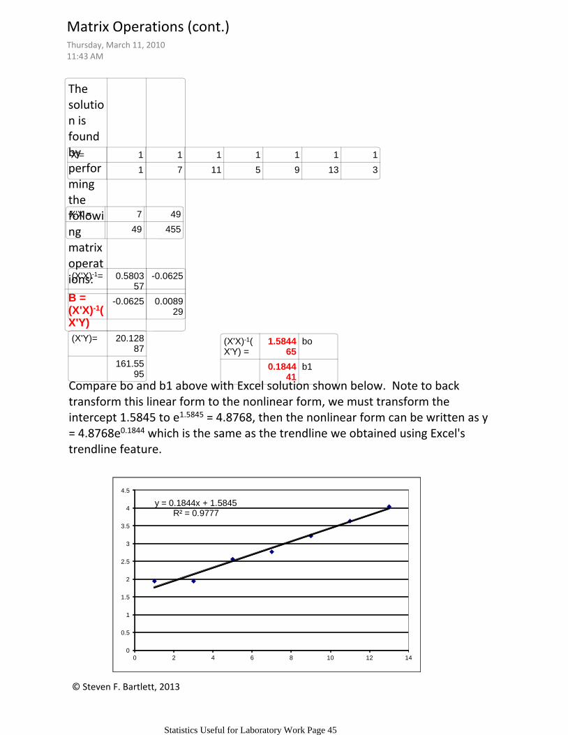
The solution is found by performing the following matrix operations:
B = (X'X)-1(X'Y)
X'= 1 1 1 1 1 1 1
1 7 11 5 9 13 3
X'X = 7 49
49 455
(X'X)-1= 0.580357
-0.0625
-0.0625 0.008929
(X'Y)= 20.12887
161.5595
(X'X)-1(X'Y) =
1.584465
bo
0.184441
b1
y = 0.1844x + 1.5845R² = 0.9777
0
0.5
1
1.5
2
2.5
3
3.5
4
4.5
0 2 4 6 8 10 12 14
Compare bo and b1 above with Excel solution shown below. Note to back transform this linear form to the nonlinear form, we must transform the intercept 1.5845 to e1.5845 = 4.8768, then the nonlinear form can be written as y = 4.8768e0.1844 which is the same as the trendline we obtained using Excel's trendline feature.
Matrix Operations (cont.)Thursday, March 11, 201011:43 AM
Statistics Useful for Laboratory Work Page 45
© Steven F. Bartlett, 2013
CVEEN 3310 Lab Safety PlanThursday, March 11, 201011:43 AM
Laboratory Safety Plan Page 46
© Steven F. Bartlett, 2013
CVEEN 3310 Lab Safety Plan (cont.)Thursday, March 11, 201011:43 AM
Laboratory Safety Plan Page 47
© Steven F. Bartlett, 2013
CVEEN 3310 Lab Safety Plan (cont.)Thursday, March 11, 201011:43 AM
Laboratory Safety Plan Page 48
© Steven F. Bartlett, 2013
CVEEN 3310 Lab Safety Plan (cont.)Thursday, March 11, 201011:43 AM
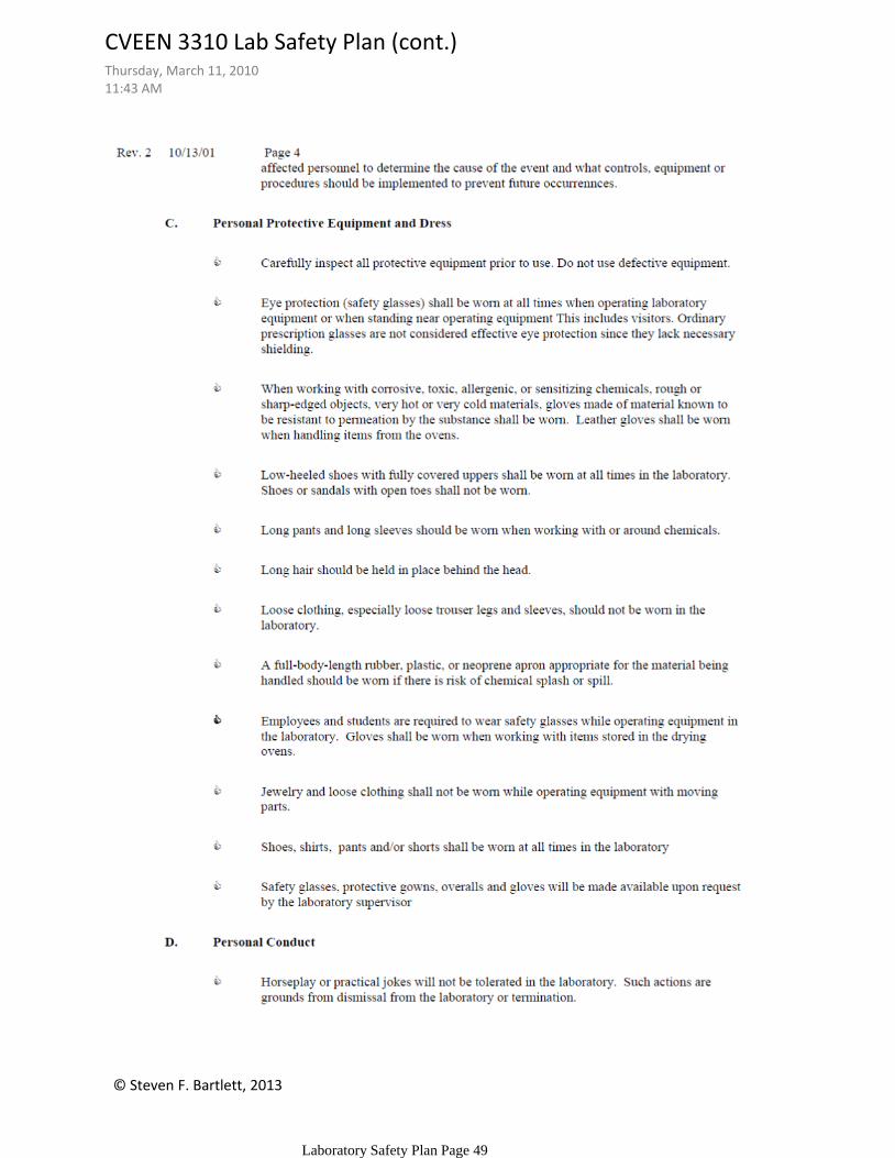
Laboratory Safety Plan Page 49

© Steven F. Bartlett, 2013
CVEEN 3310 Lab Safety Plan (cont.)Thursday, March 11, 201011:43 AM
Laboratory Safety Plan Page 50

© Steven F. Bartlett, 2013
CVEEN 3310 Lab Safety Plan (cont.)Thursday, March 11, 201011:43 AM
Laboratory Safety Plan Page 51
© Steven F. Bartlett, 2013
CVEEN 3310 Lab Safety Plan (cont.)Thursday, March 11, 201011:43 AM
Laboratory Safety Plan Page 52

© Steven F. Bartlett, 2013
CVEEN 3310 Lab Safety Plan (cont.)Thursday, March 11, 201011:43 AM
Laboratory Safety Plan Page 53

© Steven F. Bartlett, 2013
CVEEN 3310 Lab Safety Plan (cont.)Thursday, March 11, 201011:43 AM
Laboratory Safety Plan Page 54
© Steven F. Bartlett, 2013
CVEEN 3310 Lab Safety Plan (cont.)Thursday, March 11, 201011:43 AM
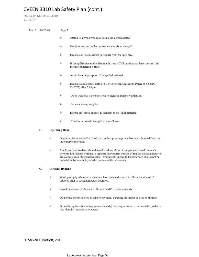
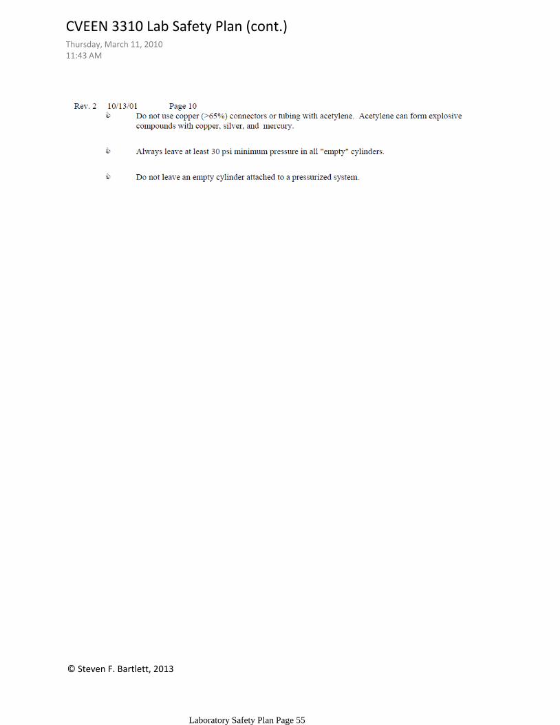
Laboratory Safety Plan Page 55
© Steven F. Bartlett, 2013
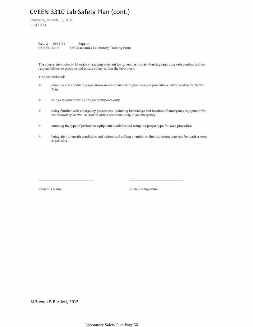
CVEEN 3310 Lab Safety Plan (cont.)Thursday, March 11, 201011:43 AM
Laboratory Safety Plan Page 56
5-cycle semi log paperWednesday, January 09, 20133:18 PM
Misc Page 57
© Steven F. Bartlett, 2013
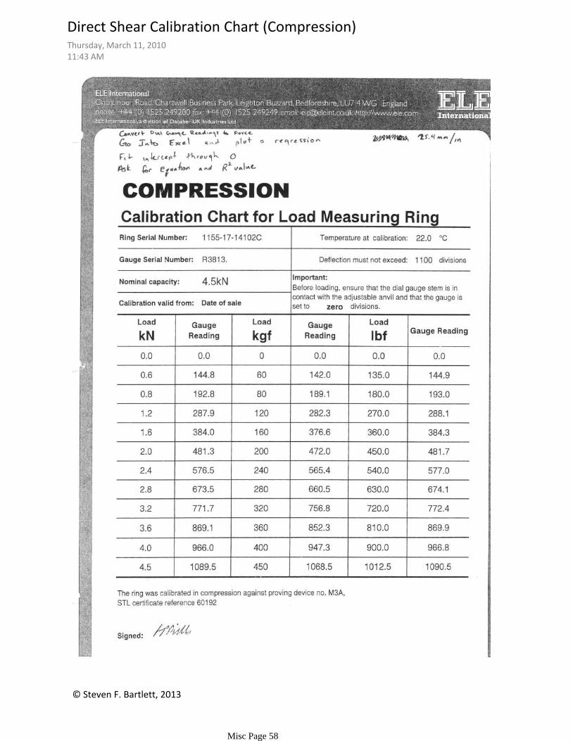
Direct Shear Calibration Chart (Compression)Thursday, March 11, 201011:43 AM
Misc Page 58
© Steven F. Bartlett, 2013
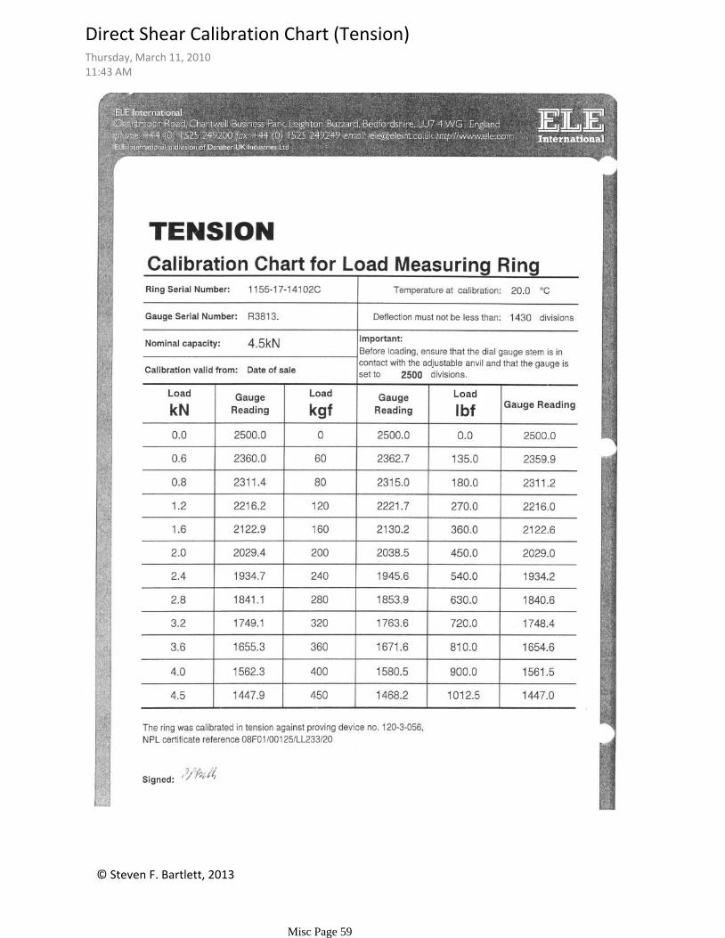
Direct Shear Calibration Chart (Tension)Thursday, March 11, 201011:43 AM
Misc Page 59

© Steven F. Bartlett, 2013
BlankThursday, March 11, 201011:43 AM
Misc Page 60