CUTTING STRATEGIES FOR FORGING DIE ......ROUGH CUT MILLING OF EXPERIMENTAL DIE CAVITIES.....34 3.1...
128
CUTTING STRATEGIES FOR FORGING DIE MANUFACTURING ON CNC MILLING MACHINES A THESIS SUBMITTED TO THE GRADUATE SCHOOL OF NATURAL AND APPLIED SCIENCES OF MIDDLE EAST TECHNICAL UNIVERSITY BY ARDA ÖZGEN IN PARTIAL FULFILLMENT OF THE REQUIREMENTS FOR THE DEGREE OF MASTER OF SCIENCE IN MECHANICAL ENGINEERING MARCH 2008
Transcript of CUTTING STRATEGIES FOR FORGING DIE ......ROUGH CUT MILLING OF EXPERIMENTAL DIE CAVITIES.....34 3.1...
CUTTING STRATEGIES FOR FORGING DIE
MANUFACTURING ON CNC MILLING MACHINES
A THESIS SUBMITTED TO THE GRADUATE SCHOOL OF NATURAL AND APPLIED SCIENCES
OF MIDDLE EAST TECHNICAL UNIVERSITY
BY
ARDA ÖZGEN
IN PARTIAL FULFILLMENT OF THE REQUIREMENTS
FOR THE DEGREE OF MASTER OF SCIENCE
IN MECHANICAL ENGINEERING
MARCH 2008
Approval of the thesis:
CUTTING STRATEGIES FOR FORGING DIE MANUFACTURING ON CNC MILLING MACHINES
submitted by ARDA ÖZGEN in partial fulfillment of the requirements for the degree of Master of Science in Mechanical Engineering, Middle East Technical University by, Prof. Dr. Canan Özgen Dean, Graduate School of Natural and Applied Sciences __________________ Prof. Dr. Kemal İDER Head of the Department, Mechanical Engineering __________________ Prof. Dr. Mustafa İlhan GÖKLER Supervisor, Mechanical Engineering Dept., METU __________________ Examining Committee Members: Prof. Dr. A. Demir Bayka Mechanical Engineering Dept., METU __________________ Prof. Dr. Mustafa İlhan GÖKLER Mechanical Engineering Dept., METU __________________ Prof. Dr. S. Engin KILIÇ Mechanical Engineering Dept., METU __________________ Prof. Dr. R. Orhan YILDIRIM Mechanical Engineering Dept., METU __________________ Prof. Dr. Can ÇOĞUN Mechanical Engineering Dept., Gazi University __________________ Date: March 27th, 2008

iii
I hereby declare that all information in this document has been obtained and presented in accordance with academic rules and ethical conduct. I also declare that, as required by these rules and conduct, I have fully cited and referenced all material and results that are not original to this work. Name, Last name: Arda Özgen Signature:
iv
ABSTRACT
CUTTING STRATEGIES FOR FORGING DIE MANUFACTURING ON CNC MILLING MACHINES
Özgen, Arda
M.Sc., Department of Mechanical Engineering
Supervisor: Prof. Dr. Mustafa İlhan Gökler
March 2008, 110 pages
Manufacturing of dies has been presenting greater requirements of geometrical
accuracy, dimensional precision and surface quality as well as decrease in costs and
manufacturing times. Although proper cutting parameter values are utilized to obtain
high geometrical accuracy and surface quality, there may exist geometrical
discrepancy between the designed and the manufactured surface profile of the die
cavities. In milling process; cutting speed, step over and feed are the main cutting
parameters and these parameters affect geometrical accuracy and surface quality of
the forging die cavities.
In this study, effects of the cutting parameters on geometrical error have been
examined on a representative die cavity profile. To remove undesired volume in the
die cavities, available cutting strategies are investigated. Feed rate optimization is
performed to maintain the constant metal removal rate along the trajectory of the
milling cutter during rough cutting process.
In the finish cutting process of the die cavities, Design of Experiment Method has
been employed to find out the effects of the cutting parameters on the geometrical
accuracy of the manufactured cavity profile. Prediction formula is derived to
estimate the geometrical error value in terms of the values of the cutting parameters.

v
Validity of the prediction formula has been tested by conducting verification
experiments for the representative die geometry and die cavity geometry of a forging
part used in industry. Good agreement between the predicted error values and the
measured error values has been observed.
Keywords: Forging Dies, Milling Process, Geometrical Error, Design of
Experiment.
vi
ÖZ
DÖVME KALIPLARININ CNC FREZE TEZGAHLARINDA ÜRETİMİ İÇİN KESİM YÖNTEMLERİ
Özgen, Arda
Yüksek Lisans, Makina Mühendisliği Bölümü
Tez Yöneticisi: Prof. Dr. Mustafa İlhan Gökler
Mart 2008, 110 sayfa
Kalıp üretiminde geometrik doğruluk, ölçüsel netlik ve yüzey kalitesi bakımından
daha fazla gereksinimlerin yanında, maliyetlerde ve üretim zamanlarında azalma
talep edilmektedir. Yüksek geometrik doğruluğu ve yüzey kalitesini elde etmek için
uygun kesim parametre değerleri uygulansa bile, tasarlanan ve imal edilen kalıp
boşluğunun yüzey profili arasında geometrik farklılıklar bulunabilir. Frezeleme
işleminde; kesim hızı, yanal adım ve takım ilerlemesi esas kesim parametreleri olup,
dövme kalıplarının geometrik doğruluğunu ve yüzey kalitesini bu parametreler
etkiler.
Bu çalışmada, kesim parametrelerinin geometrik hata üzerine etkileri temsili bir kalıp
boşluğu profili üzerinde incelenmiştir. Kalıp boşluklarındaki istenmeyen hacmi
boşaltmak için mevcut kesim stratejileri araştırılmıştır. Kaba kesim işlemi sırasında,
kesici takımın yolu boyunca sabit talaş kaldırma hızını sağlamak için takım ilerleme
optimizasyonu yapılmıştır.
Kalıp boşluklarının nihai kesim işleminde; kesim parametrelerinin imal edilen boşluk
profilinin geometrik doğruluğu üzerine etkilerinin bulunması amacıyla, deneysel
tasarım metodu kullanılmıştır. Geometrik hatanın kesim parametrelerinin değerleri
cinsinden hesaplanabilmesi için tahmin formülü çıkarılmıştır. Tahmin formülünün

vii
geçerliliği, temsili kalıp geometrisi ve endüstride kullanılan bir dövme parçasının
kalıp boşluğu geometrisi için doğrulama deneyleri yapılarak test edilmiştir. Tahmin
edilen hata değerleri ile ölçülen hata değerleri arasında iyi uyum gözlemlenmiştir.
Anahtar Kelimeler: Dövme Kalıpları, Frezeleme İşlemi, Geometrik Hata, Deney
Tasarımı.

viii
To whom, they make this study
possible with their contributions

ix
ACKNOWLEDGEMENTS
I would like to express my deepest gratitude to my supervisor Prof. Dr. Mustafa
İlhan Gökler for his guidance, advice, criticism, encouragement and insight
throughout the study.
The author was supported by The Scientific and Technological Research Council of
Turkey (TÜBİTAK) with National Scholarship Program for MSc Students (Program
no: 2210).
I express sincere appreciation to Mechanical Engineering Department of METU for
the facilities conducted in the study.
I wish to thank to METU-BİLTİR Research and Application Center, AKSAN Steel
Forging Company for the research applications performed during the experimental
study.
I also would like to thank to my senior colleagues Kazım Arda Çelik, Mehmet
Maşat, Sevgi Saraç, İlker Durukan for their valuable support and assistance.
Special thanks go to my colleagues, Hüseyin Öztürk, Cihat Özcan, Özgür Cavbozar,
Ulaş Göçmen, Ali Murat Kayıran, Halit Şahin, Ali Demir and Hüseyin Ali Atmaca
for their endless efforts and aids.
I am deeply indebt to my parents, Ayfer and Turgut Özgen for their encouragement
and faith in me.
x
TABLE OF CONTENTS
ABSTRACT................................................................................................................ iv
ÖZ ..................................................................................................................... vi
ACKNOWLEDGEMENTS ........................................................................................ ix
TABLE OF CONTENTS............................................................................................. x
LIST OF TABLES ....................................................................................................xiii
LIST OF FIGURES ................................................................................................... xv
LIST OF SYMBOLS ..............................................................................................xviii
CHAPTER
1. INTRODUCTION.................................................................................................... 1
1.1 Forging Process............................................................................................. 1
1.2 Precision Forging .......................................................................................... 2
1.3 Forging Die Manufacturing .......................................................................... 5
1.4 CNC Milling vs. EDM Process in Die Manufacturing ................................. 8
1.5 Importance of Geometric Accuracy and Manufacturing Time in Forging
Die Manufacturing ........................................................................................ 9
1.6 Some Previous Studies................................................................................ 11
1.7 Scope of the Thesis ..................................................................................... 12
2. GEOMETRIC DIMENSIONING AND TOLERANCING IN FORGING DIES. 14
2.1 Definition of Geometric Dimensioning and Tolerancing ........................... 14
2.2 Feature Control Frame in GD&T................................................................ 16
xi
2.3 Advantages of GD&T over Coordinate Dimensioning and Tolerancing.... 17
2.4 Profile Tolerancing ..................................................................................... 19
2.5 Dimensional Tolerances of Dies ................................................................. 23
2.6 Design Considerations of Forging Dies ...................................................... 25
2.6.1 Fillet and Corner Radii....................................................................... 26
2.6.2 Draft Angle ........................................................................................ 27
2.7 Determination of the Experimental Geometry for the Study ...................... 28
3. ROUGH CUT MILLING OF EXPERIMENTAL DIE CAVITIES...................... 34
3.1 Importance of Rough Cutting Operations in Forging Die Manufacturing.. 34
3.2 Cutting Parameters for Rough Machining .................................................. 35
3.3 Constant Metal Removal Rate in Rough Cut.............................................. 38
3.4 Tool Path Generation for Rough Machining............................................... 39
3.5 Deficiencies of Spiral Tool Path ................................................................. 43
3.6 Rough Cutting Parameters for the Selected Geometry ............................... 45
3.7 Rough Cut Optimization ............................................................................. 47
4. FINISH CUT MILLING OF EXPERIMENTAL DIE CAVITIES ....................... 52
4.1 Three Level Factorial Design...................................................................... 52
4.2 Finish Cut Experiments and Experimental Details ..................................... 53
4.3 Geometrical Measurement .......................................................................... 60
4.3.1 Measurement Setup............................................................................ 60
4.3.2 Scanning Technique on CMM ........................................................... 61
4.3.3 Geometrical Error Analysis................................................................ 63
5. ANALYSIS OF THE EXPERIMENTS AND DERIVATION
OF GEOMETRICAL ERROR PREDICTION FORMULA ................................. 67
5.1 Geometrical Error Analysis of the First Set of Experiments ...................... 67

xii
5.2 Geometrical Error Analysis of the Second Set of Experiments.................. 73
5.3 Geometrical Error Prediction Formula........................................................ 79
5.4 Verification Analysis for the Finish Cut Experiments................................ 80
5.5 Case Study................................................................................................... 82
6. CONCLUSION...................................................................................................... 86
6.1 Conclusions ................................................................................................. 86
6.2 Recommendations for Future Work............................................................ 89
REFERENCES........................................................................................................... 90
APPENDICES
A. MAZAK VARIAXIS 630-5X CNC MILLING CENTER ................................... 94
B. DIEVAR PREMIUM HOT WORK TOOL STEEL ............................................. 96
B.1 General ........................................................................................................ 96
B.2 Hot Work Applications ............................................................................... 97
B.3 Properties .................................................................................................... 97
C. PROPERTIES OF THE CUTTING TOOLS ........................................................ 99
USED IN ROUGH AND FINISH CUT MILLING .............................................. 99
C.1 General ........................................................................................................ 99
C.2 Cutting Data Recommendations of Dievar Tool Steel for
Carbide Tools ............................................................................................ 100
D. ORIGINAL TOOL PATH VS. OPTIMIZED TOOL PATH.............................. 101
E. REGRESSION ANALYSIS OF THE FINISH CUT EXPERIMENTS ............. 109
xiii
LIST OF TABLES
TABLES
Table 1.1 Comparison of EDM process with CNC milling application ...................... 9
Table 2.1 Tolerance symbols with their descriptions................................................. 15
Table 2.2 Forging tolerances for length, width, and height ....................................... 25
Table 2.3 Recommendations for minimum fillet and corner radii............................. 27
Table 2.4 List of the parts forged by 1000 ton press at Aksan Steel
Forging Company ...................................................................................... 29
Table 3.1 Cutting strategies vs. cycle time ................................................................ 43
Table 3.2 Rough cutting parameters .......................................................................... 46
Table 3.3 Cutting coordinates of die cavities wrt reference coordinate..................... 51
Table 4.1 Cutting data recommendations for end milling.......................................... 54
Table 4.2 Selected factors and levels for the first set of finish cut experiments........ 58
Table 4.3 Selected factors and levels for the second set of finish cut experiments ... 58
Table 4.4 Design matrix for the experiments............................................................. 59
Table 5.1 Results of the first set of experiments........................................................ 69
Table 5.2 Comparison of geometrical error values with production time values ...... 73
Table 5.3 Results of the second set of experiments ................................................... 75
Table 5.4 Comparison of geometrical error values with production time values ...... 79
Table 5.5 Results of the verification experiments...................................................... 80
Table 5.6 Comparison of predicted error values with measured error values ........... 82

xiv
Table 5.7 Cutting strategies vs. cycle time ................................................................ 83
Table 5.8 Results of the case study ............................................................................ 84
Table 5.9 Comparison of predicted error values with measured error values ........... 85
Table B.1 General characteristics of Dievar .............................................................. 96
Table B.2 Physical properties of Dievar .................................................................... 97
Table B.3 Mechanical properties of Dievar ............................................................... 98
Table C.1 Cutting data recommendations for end milling....................................... 100
xv
LIST OF FIGURES
FIGURES
Figure 1.1 Precisely forged parts ................................................................................. 3
Figure 1.2 Precision and conventionally forged components ...................................... 4
Figure 1.3 Flow diagram of the die manufacturing processes of
Aksan Steel Forging Company ................................................................... 6
Figure 1.4 Lead times in manufacturing of dies .......................................................... 7
Figure 2.1 Feature control frame................................................................................ 17
Figure 2.2 Traditional plus or minus tolerancing system........................................... 18
Figure 2.3 Bilateral tolerance on a profile ................................................................. 20
Figure 2.4 Unilateral tolerance outside on a profile................................................... 20
Figure 2.5 Unilateral tolerance inside on a profile..................................................... 21
Figure 2.6 Unequally distributed bilateral tolerance on a profile .............................. 21
Figure 2.7 All around tolerance symbol..................................................................... 22
Figure 2.8 Between tolerance symbol........................................................................ 22
Figure 2.9 All over tolerance symbol......................................................................... 23
Figure 2.10 Corner radii and fillet radii in forging dies............................................. 26
Figure 2.11 Types of draft angles in forging dies ...................................................... 28
Figure 2.12 Entities of the designed profile ............................................................... 30
Figure 2.13 Profile used in the experiments .............................................................. 31
Figure 2.14 Experimental die cavity geometry .......................................................... 32

xvi
Figure 2.15 Profile tolerance of the experimental cavity........................................... 33
Figure 3.1 Up and down milling ................................................................................ 37
Figure 3.2 Parameters of metal removal rate ............................................................. 39
Figure 3.3 NC programming [10] .............................................................................. 40
Figure 3.4 Pro/Engineer Wildfire 3 cutting strategy library ...................................... 41
Figure 3.5 Type spiral tool path ................................................................................. 42
Figure 3.6 First deficiency of spiral tool path ............................................................ 44
Figure 3.7 Second deficiency of spiral tool path........................................................ 45
Figure 3.8 Sample of optimized code ........................................................................ 48
Figure 3.9 Geometrical distribution of the die cavities with experiment numbers.... 50
Figure 3.10 Datum surfaces for reference coordinate................................................ 50
Figure 4.1 Treatment combinations in 32 design ....................................................... 52
Figure 4.2 Scallop formations during ball nose finishing ......................................... 55
Figure 4.3 Tool path with 0.10 mm step over ............................................................ 56
Figure 4.4 Tool path with 0.20 mm step over ............................................................ 56
Figure 4.5 Tool path with 0.30 mm step over ............................................................ 57
Figure 4.6 CMM used in the study ............................................................................ 60
Figure 4.7 Scanning technique on CMM ................................................................... 62
Figure 4.8 Scanning directions................................................................................... 63
Figure 4.9 Geometrical error analysis process........................................................... 64
Figure 4.10 Geometrical error measurement ............................................................. 65
Figure 5.1 Design matrix for the first set of experiments .......................................... 67
Figure 5.2 Photograph of the first set of experiments................................................ 68
Figure 5.3 Main effect plot of the first input parameter............................................. 70
Figure 5.4 Main effect plot of the second input parameter ........................................ 70
xvii
Figure 5.5 Interaction effect plot of the input parameters.......................................... 71
Figure 5.6 Surface plot of the response variable geometrical error ........................... 72
Figure 5.7 Design matrix for the second set of experiments ..................................... 73
Figure 5.8 Photograph of the second set of experiments ........................................... 74
Figure 5.9 Main effect plot of the first input parameter............................................. 76
Figure 5.10 Main effect plot of the second input parameter ...................................... 76
Figure 5.11 Interaction effect plot of the input parameters........................................ 77
Figure 5.12 Surface plot of the response variable geometrical error ......................... 78
Figure 5.13 Photograph of the verification experiments............................................ 81
Figure 5.14 Die and forging part geometries for the case study ................................ 83
Figure 5.15 Photograph of the case study .................................................................. 84
Figure A.1 Mazak Variaxis 630-5x milling center .................................................... 94
Figure C.1 Dimensional properties of the rough cutter.............................................. 99
Figure C.2 Dimensional properties of the finish cutter............................................ 100

xviii
LIST OF SYMBOLS
SYMBOLS
ap : Axial depth of cut
ae : Radial depth of cut (i.e. Step over)
Vf : Feed rate
Vf' : Optimized feed rate
Vc : Cutting speed
ft : Feed per tooth
nt : Number of cutting edges
N : Spindle speed
D : Tool diameter
R : Tool radius
Zw : Metal removal rate
Sh : Scallop height
k : Number of factors
β : Coefficients of linear regression model
Z : Real geometrical error
Z' : Predicted geometrical error
Ap : Effective flute length
L : Tool length
H : Flute length
1
CHAPTER 1
INTRODUCTION
1.1 Forging Process
Forging is a metal forming process in which a piece of metal is shaped to the desired
form by plastic deformation. The process usually includes sequential deformation
steps to the final shape. In forging process, compressive force may be provided by
means of manual or power hammers, mechanical, hydraulic or special forging
presses. The process is normally but not always, performed hot by preheating the
metal to a desired temperature before it is worked.
Compared to all manufacturing processes, forging technology has a special place
because it helps to produce parts of superior mechanical properties with minimum
waste of material. Forging process gives the opportunity to produce complex parts
with desired directional strength, refining the grain structure and developing the
optimum grain flow, which imparts desirable directional properties. Forging products
are free from undesirable internal voids and have the maximum strength in the vital
directions as well as a maximum strength to weight ratio [1].
Forging process can be classified into three groups as:
1. According to the forging temperature
• Cold forging
• Warm forging
2
• Hot forging
2. According to type of machine used
• Mechanical presses
• Hydraulic presses
• Hammers
• Screw presses
3. According to the type of die set
• Open die forging
• Closed die forging
Descriptions, advantages and disadvantages of these can be found in several
literatures [1].
1.2 Precision Forging
Precision forging is a kind of closed die forging and normally means “close to final
form” or “close tolerance” forging. It is not a special technology, but a refinement of
existing techniques to a point where the forged part can be used with little or no
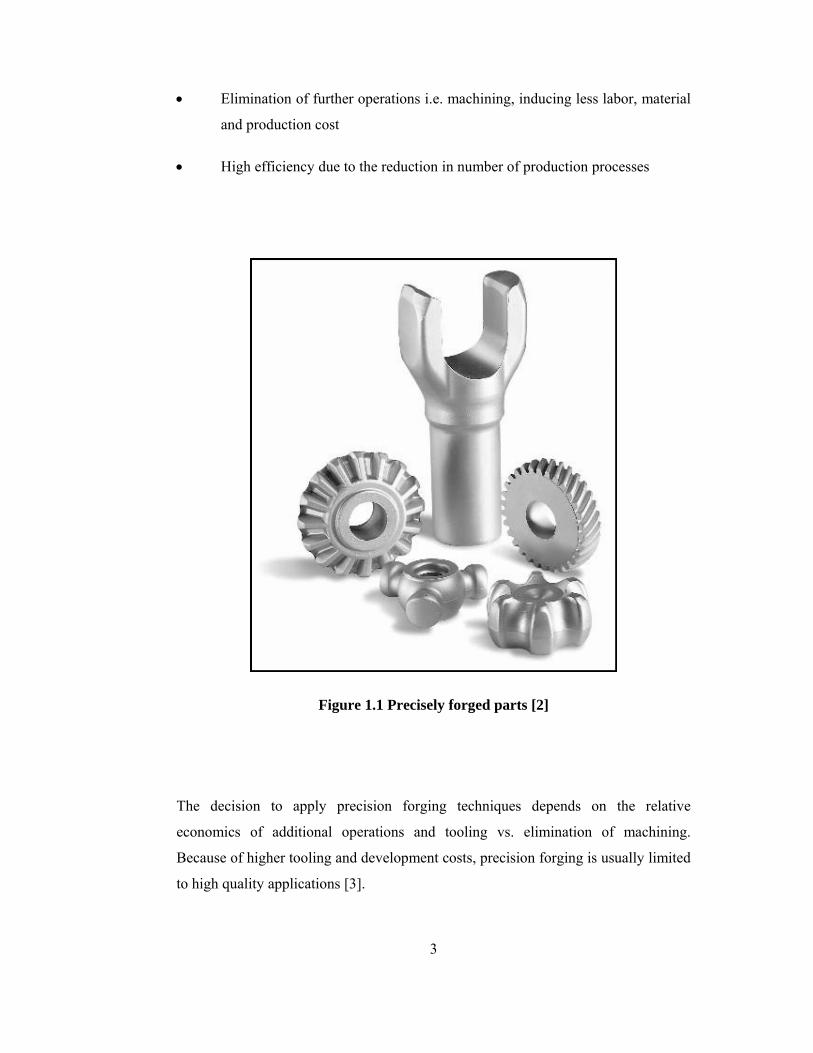
subsequent machining. Some examples of precisely forged parts are given in Figure
1.1.
In precision forging process, improvements cover not only the forging method itself
but also preheating, lubrication, and temperature control practices. Major advantages
of precision forging can be summarized as:
• Reduction in material waste
• More uniform fiber orientation providing superior strength values
3
• Elimination of further operations i.e. machining, inducing less labor, material
and production cost
• High efficiency due to the reduction in number of production processes
Figure 1.1 Precisely forged parts [2]
The decision to apply precision forging techniques depends on the relative
economics of additional operations and tooling vs. elimination of machining.
Because of higher tooling and development costs, precision forging is usually limited
to high quality applications [3].
4
As the process name suggests, precision forging dies require better geometrical
accuracy when compared with conventional forging processes. End products of
precision forging are net-shape or near net-shape. Therefore, more attention should
be paid to the manufacturing steps of precision die manufacturing.
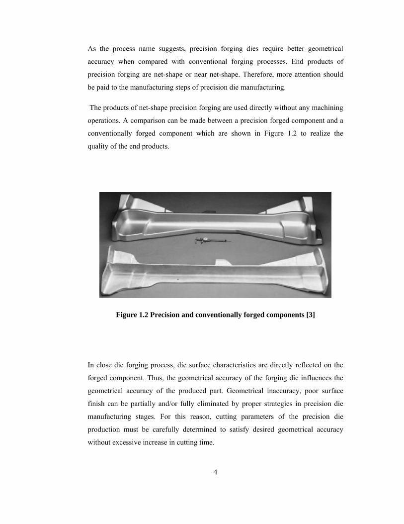
The products of net-shape precision forging are used directly without any machining
operations. A comparison can be made between a precision forged component and a
conventionally forged component which are shown in Figure 1.2 to realize the
quality of the end products.
Figure 1.2 Precision and conventionally forged components [3]
In close die forging process, die surface characteristics are directly reflected on the
forged component. Thus, the geometrical accuracy of the forging die influences the
geometrical accuracy of the produced part. Geometrical inaccuracy, poor surface
finish can be partially and/or fully eliminated by proper strategies in precision die
manufacturing stages. For this reason, cutting parameters of the precision die
production must be carefully determined to satisfy desired geometrical accuracy
without excessive increase in cutting time.
5
Die manufacturers aim to obtain high geometrical accuracy and surface quality in die
cavities by utilizing proper cutting strategies and parameters; however, there may
exist geometrical discrepancy between surface profile of the designed and the
manufactured die cavity. The effects of the cutting parameters on geometrical
accuracy of a specific cavity profile can be analyzed to minimize this geometrical
discrepancy.
1.3 Forging Die Manufacturing
Forging die manufacturing requires various affiliated operations that should be
separately considered. It would be beneficial to examine real applications of forging
die manufacturing to acquire comprehensive information about processes. Thus,
Aksan Steel Forging Company in Ankara is chosen as the reference company to
investigate current practices in forging die manufacturing [4].
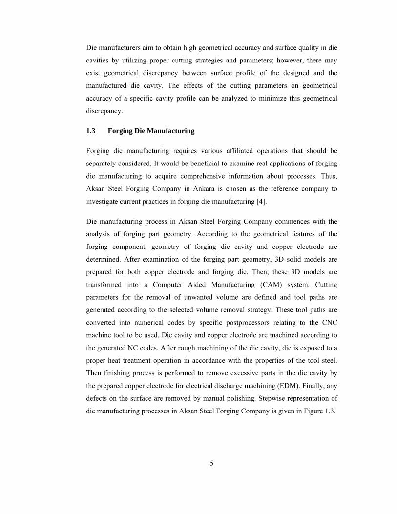
Die manufacturing process in Aksan Steel Forging Company commences with the
analysis of forging part geometry. According to the geometrical features of the
forging component, geometry of forging die cavity and copper electrode are
determined. After examination of the forging part geometry, 3D solid models are
prepared for both copper electrode and forging die. Then, these 3D models are
transformed into a Computer Aided Manufacturing (CAM) system. Cutting
parameters for the removal of unwanted volume are defined and tool paths are
generated according to the selected volume removal strategy. These tool paths are
converted into numerical codes by specific postprocessors relating to the CNC
machine tool to be used. Die cavity and copper electrode are machined according to
the generated NC codes. After rough machining of the die cavity, die is exposed to a
proper heat treatment operation in accordance with the properties of the tool steel.
Then finishing process is performed to remove excessive parts in the die cavity by
the prepared copper electrode for electrical discharge machining (EDM). Finally, any
defects on the surface are removed by manual polishing. Stepwise representation of
die manufacturing processes in Aksan Steel Forging Company is given in Figure 1.3.
6
Figure 1.3 Flow diagram of the die manufacturing processes of
Aksan Steel Forging Company
Application of EDM process necessitates manual polishing in the die cavities since
micro cracks and nano cracks are formed at the surface layer which is produced by
7
the copper electrode. The formation of these cracks is exactly related with EDM in
which electrically conductive material is removed by means of rapid and repetitive
spark discharges resulting from local explosion of a dielectric liquid. These spark
discharges are produced by applying a voltage between copper electrode and
workpiece [5]. EDM process forms a layer as a result of the solidification of a melted
zone. As a consequence of the rapid quenching process, micro cracks and nano
cracks are formed at the surface of the layer [6]. As the hardness is higher in this
layer, this layer becomes more brittle and the micro cracks may lead to crack
propagation during forging process on die surfaces. As a result of these, polishing
should be applied on die surfaces to remove this hardened layer after EDM process.
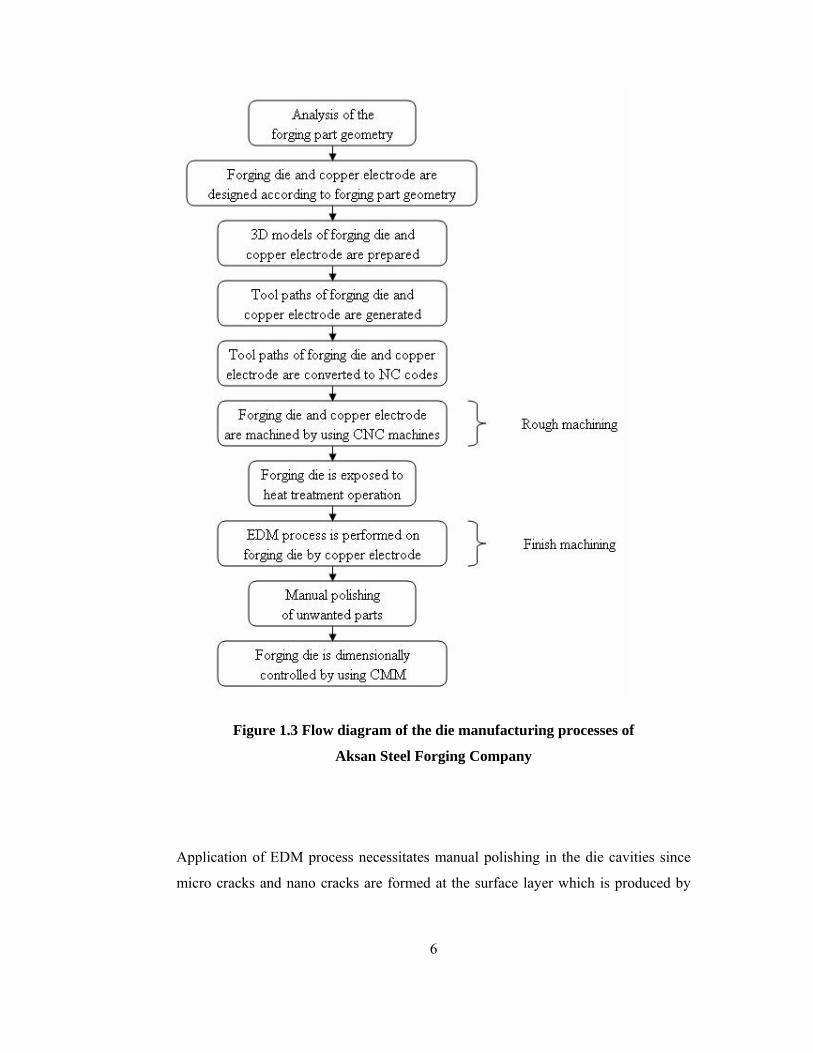
Figure 1.4 Lead times in manufacturing of dies [7]
It can be concluded from Figure 1.4 that, polishing time constitutes 20-30% of total
manufacturing time of forging die production. It is obvious that reduction in any of
8
the steps of die manufacturing process, will improve efficiency of the whole
operation in cost wise and time wise. For this reason, cutting strategies should be
developed and numerical codes should be optimized in such a way that no additional
application is required in the die cavity after CNC machining operation. At that point
it should always be taken into account that a compromise must be achieved between
machining times and final surface finish of the die cavity. As a consequence of this
compromise, surface finish can be greatly improved, reducing and/or eliminating
manual polishing, that may account for up to 20-30% of the total time spent in the
die manufacturing process.
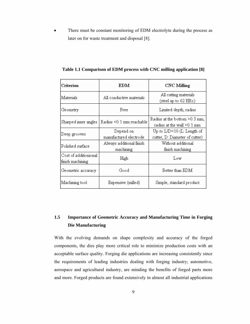
1.4 CNC Milling vs. EDM Process in Die Manufacturing
Nowadays CNC milling technology is a basic constituent part of every modern tool
making company. According to the objective model for cavity manufacturing
technology, where milling tool, die and product related parameters are considered,
CNC milling technology is prevalently replacing classical die sinking EDM
applications. As a consequence of these, for each die cavity, it has to be ascertain,
which technology CNC milling plus EDM finishing or CNC milling alone is the
most advantageous. In Table 1.1, advantages, disadvantages as well as limits of the
EDM and CNC milling are presented.
For the selection of the most appropriate die cavity manufacturing technology,
energy consumption and ecology are of a great importance too. It is well known that
the EDM process has a very high level of energy consumption. Therefore, it should
be used only in cases where, regarding product, milling tool shape or die related
properties does not allow the CNC milling applications.
From ecology point of view CNC milling technology is prevailing EDM for the
following reasons:
• Technology using less energy is much friendlier to the environment.
• Permanent decrease of cutting lubricants and coolants leads to dry machining.
9
• There must be constant monitoring of EDM electrolyte during the process as
later on for waste treatment and disposal [8].
Table 1.1 Comparison of EDM process with CNC milling application [8]
1.5 Importance of Geometric Accuracy and Manufacturing Time in Forging
Die Manufacturing
With the evolving demands on shape complexity and accuracy of the forged
components, the dies play more critical role to minimize production costs with an
acceptable surface quality. Forging die applications are increasing consistently since
the requirements of leading industries dealing with forging industry; automotive,
aerospace and agricultural industry, are minding the benefits of forged parts more
and more. Forged products are found extensively in almost all industrial applications
10
requiring strength, reliability, toughness and quality. Forged components are
economically attractive because of their inherent superior reliability, improved
tolerance capability, and higher efficiency with which forging products can be
machined and further processed by automated methods.
Nowadays, manufacturing of dies is more and more competitive, presenting greater
requirements of dimensional precision and surface roughness as well as a decrease in
costs and manufacturing times [9]. In order to achieve desired surface quality on
forged components and to manufacture forging dies in tight tolerances without
increasing production time significantly, cutting conditions and parameters must be
determined diligently.
The current trend of die manufacturing is determination of cutting conditions to
obtain the closest dimensional and geometrical accuracy resulted in minimization of
further operations which is mostly manual polishing. However, variety in the
geometry of produced components makes it difficult for die manufacturers to select
the optimum operational conditions in a repetitive and reliable way. Great number of
factors, which is necessary to take into account, makes it really difficult to select the
optimum operational conditions properly. These factors can be summarized as,
geometric specifications of the part, geometry of the part before being machined,
material of the part, position of the part in the machine tool, fixture system of the
part, method of machining, type of the tool holder, type of the cutting tool, cutting
parameters (i.e. axial depth of cut, radial depth of cut, feed rate and spindle speed),
cutting fluid and capability of CAM system [9]. Among these factors, only cutting
parameters are fully numerically controlled and adjustable. Therefore, these
parameters have substantial contribution to lessen the manufacturing times when
compared with the effects of other factors. In order to minimize the cutting time of
the manufacturing processes and obtain geometrical accuracy in accordance with
product specifications, the most suitable manufacturing conditions for each operation
must be carefully selected. While, only the cutting parameters (i.e. depth of cut, feed
rate, cutting speed) are generally taken into account, each element involved in the
machining process has a considerable influence on the final result of that process.
11
One can see that it is necessary to have a deeper knowledge about the optimum
operation conditions, which will permit to assure a desired dimensional precision
with an acceptable production time.
1.6 Some Previous Studies
Various factors of CNC milling technology influence the quality of the final part and
its manufacturing economy. Tool materials, type of the tool holder and control
system of the machine tool, cutting parameters (depth of cut, feed and cutting speed)
and axial capability of the machine tool are the key factors directly affecting the
geometrical accuracy of the produced part. Among these factors, only cutting
parameters are suitable for any kind of modifications without altering the current
installation. Additional investments to increase performance of the machine tool (tool
and axial capability wise) are generally less favorable by the manufacturers.
Therefore, many research activities have been performed either to optimize current
process or develop new approaches to maximize the process efficiency.
Individually analyzing the effects of each of these factors on the final result has
generated much interest. Various research studies have been recently conducted in
which one of the previously mentioned factors has been correlated with die surface
quality. J. Vivancos et al [3], L.N. Lopez de Lacalle et al [11] have worked on steel
machining and R.T. Coelho et al [12] dealed with aluminum alloys machining.
However, only few researchers have analyzed the relationship between these factors
and geometrical accuracy. Similarly, the influence of these factors on production
time has been analyzed in very few cases.
Another key objective of the recent researches is the optimization of cutting
parameters in high speed machining, and in this field a great variety of work can be
found. A. Kaldos et al [13] based on optimization for aluminum alloys machining
and W.T. Chien et al [14], H. Juan et al [15] and L.N. Lopez de Lacalle et al [16]
studied optimization of cutting parameters for steel machining.
Many researchers have also worked on the optimization of feed rate and tool path
strategy to achieve improvements on production time. R. Salami et al [17] dealed
12
with feed rate optimization for 3-axis ball-end milling of sculptured surfaces and
Jenq Shyong By Chen et al [18] studied feed rate optimization and tool profile
modification for the high efficiency ball-end milling process. Manuel Monreal and
Ciro A. Rodriguez [19] focused on influence of tool path strategy on the cycle time
of CNC milling operations.
To enhance die manufacturing capabilities of METU-BİLTİR Research and
Application Center, a post processor with a simulation program for Mazak Variaxis
630-5x [20] and a methodology for prediction of surface roughness on curved
cavities [21] have been developed so far by the members of the center.
1.7 Scope of the Thesis
Recent requirements of die and mould manufacturing can be summarized as:
maintaining geometrically accurate and high quality die surfaces as well as reduction
in production time. In order to decrease production time of die manufacturing
processes and achieve geometrical accuracy in accordance with product
specifications, optimum cutting parameters for rough cutting and finish cutting
operations must be accurately selected. By selecting a fixed feed rate based upon the
maximum force, tool is saved but very often it results in extra machining time in
rough cutting operations, which reduces productivity. By optimizing the feed rate,
both objectives of saving the tool and also reducing machining time thereby increase
in productivity can be achieved.
For the finish cutting operations, attaining geometrically accurate products with
acceptable surface quality in a reasonable production time is the common objective
of today’s die manufacturers. Therefore, experimental analysis dealing with the
effects of the cutting parameters on geometrical error and production time would be
beneficial for the determination of these parameters. The main objective of this
particular study is to find out geometrical discrepancy between CAD model of a die
cavity and a manufactured die cavity by utilizing various cutting parameter values
for the finish cut operation of precision forging dies.
13
In Chapter 1, brief information about forging die manufacturing and significance of
geometrical accuracy in die manufacturing have been presented. Details of
geometrical dimensioning and tolerancing will be examined and geometrical
requirements of precision forging dies will be clarified in Chapter 2. According to
these specifications, an experimental die cavity geometry covering major surface
variations of forging dies will be defined for the experimental study.
In Chapter 3, optimum cutting strategy for rough machining of the defined
experimental die cavity geometry will be investigated and feed rate optimization will
be performed on the generated tool path. Details of the experimental analysis for
finish cutting operation and geometrical error analysis for the manufactured die
cavity will be explained in Chapter 4.
Effects of the cutting parameters on the geometrical error of the surface profile and
the production time will be handled in Chapter 5. Prediction formula to estimate
geometrical error in terms of the values of the cutting parameters will also be derived
in this chapter. Verification experiments for the representative die cavity geometry
and cavity geometry of a forging part used in industry will be performed to check the
validity of the acquired formula.
Finally, conclusion and recommendations for future work will be presented in
Chapter 6.
14
CHAPTER 2
GEOMETRIC DIMENSIONING AND TOLERANCING IN FORGING DIES
In this chapter, brief information about geometric dimensioning and tolerancing has
been presented to provide background knowledge for the current study. The design
considerations for forging die cavities have been given to relate geometric
dimensioning and tolerancing with forging die cavity design. Finally, an
experimental cavity profile which is required for the studies conducted in the
following chapters has been determined.
2.1 Definition of Geometric Dimensioning and Tolerancing
Geometric dimensioning and tolerancing (GD&T) is a symbolic language. It is used
to define the nominal geometry of parts and assemblies, to define the allowable
variation in form and possibly size of individual features, and to define the allowable
variation between features [22]. The features toleranced with GD&T reflect the
actual relationship between mating parts. Drawings with properly applied geometric
tolerancing provide the best opportunity for uniform interpretation and cost effective
assembly [23].
GD&T is a design tool. Before designers can properly apply geometric tolerancing,
they must carefully consider the fit and function of each feature of every part.
GD&T, in effect, serves as a checklist to remind the designers to consider all aspects
of each feature. Properly applied geometric tolerancing insures that every part will
assemble every time. Geometric tolerancing allows the designers to specify the
maximum available tolerance and consequently, design the most economical parts
[23].
15
GD&T scheme identifies all applicable datums, which are reference surfaces, and the
features being controlled to these datums. A properly toleranced drawing is not only
a picture that communicates the size and shape of the part, but it also tells a story that
explains the tolerance relationships between features [23].
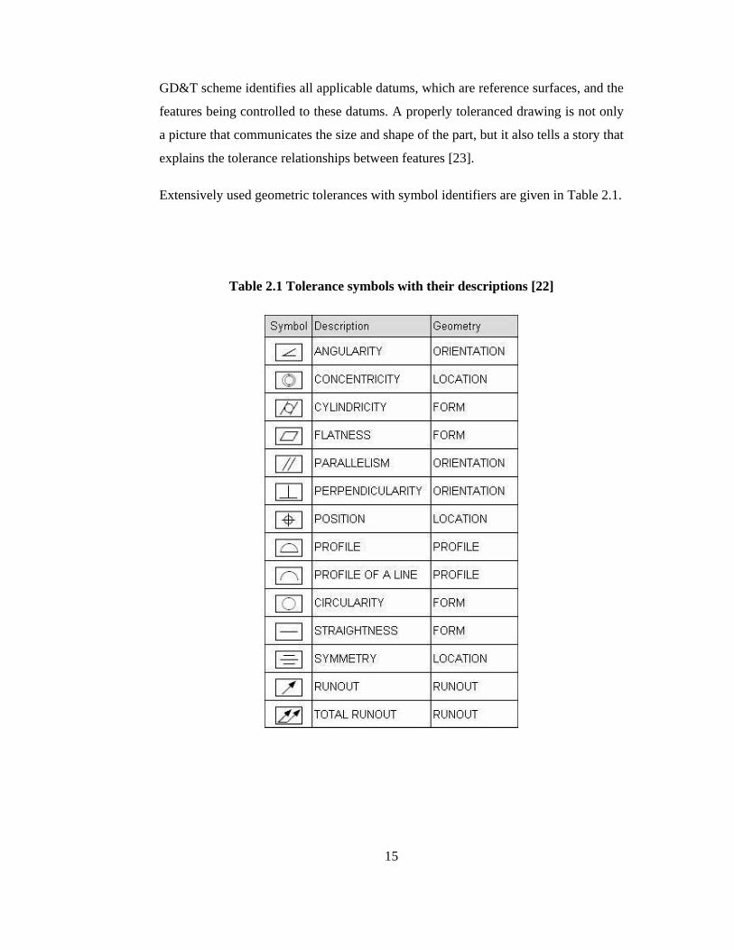
Extensively used geometric tolerances with symbol identifiers are given in Table 2.1.
Table 2.1 Tolerance symbols with their descriptions [22]
16
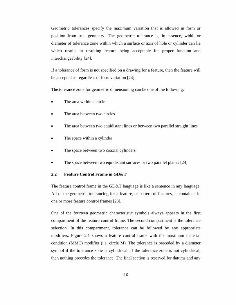
Geometric tolerances specify the maximum variation that is allowed in form or
position from true geometry. The geometric tolerance is, in essence, width or
diameter of tolerance zone within which a surface or axis of hole or cylinder can lie
which results in resulting feature being acceptable for proper function and
interchangeability [24].
If a tolerance of form is not specified on a drawing for a feature, then the feature will
be accepted as regardless of form variation [24].
The tolerance zone for geometric dimensioning can be one of the following:
• The area within a circle
• The area between two circles
• The area between two equidistant lines or between two parallel straight lines
• The space within a cylinder
• The space between two coaxial cylinders
• The space between two equidistant surfaces or two parallel planes [24]
2.2 Feature Control Frame in GD&T
The feature control frame in the GD&T language is like a sentence in any language.
All of the geometric tolerancing for a feature, or pattern of features, is contained in
one or more feature control frames [23].
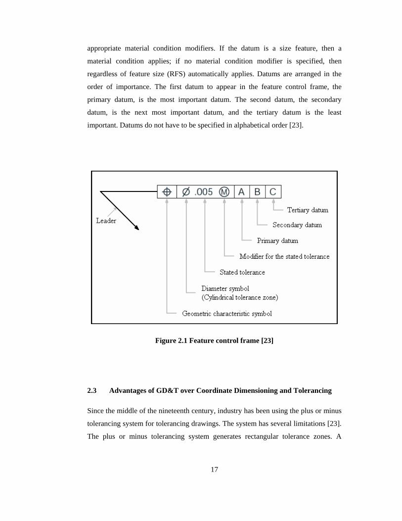
One of the fourteen geometric characteristic symbols always appears in the first
compartment of the feature control frame. The second compartment is the tolerance
selection. In this compartment, tolerance can be followed by any appropriate
modifiers. Figure 2.1 shows a feature control frame with the maximum material
condition (MMC) modifier (i.e. circle M). The tolerance is preceded by a diameter
symbol if the tolerance zone is cylindrical. If the tolerance zone is not cylindrical,
then nothing precedes the tolerance. The final section is reserved for datums and any
17
appropriate material condition modifiers. If the datum is a size feature, then a
material condition applies; if no material condition modifier is specified, then
regardless of feature size (RFS) automatically applies. Datums are arranged in the
order of importance. The first datum to appear in the feature control frame, the
primary datum, is the most important datum. The second datum, the secondary
datum, is the next most important datum, and the tertiary datum is the least
important. Datums do not have to be specified in alphabetical order [23].
Figure 2.1 Feature control frame [23]
2.3 Advantages of GD&T over Coordinate Dimensioning and Tolerancing
Since the middle of the nineteenth century, industry has been using the plus or minus
tolerancing system for tolerancing drawings. The system has several limitations [23].
The plus or minus tolerancing system generates rectangular tolerance zones. A
18
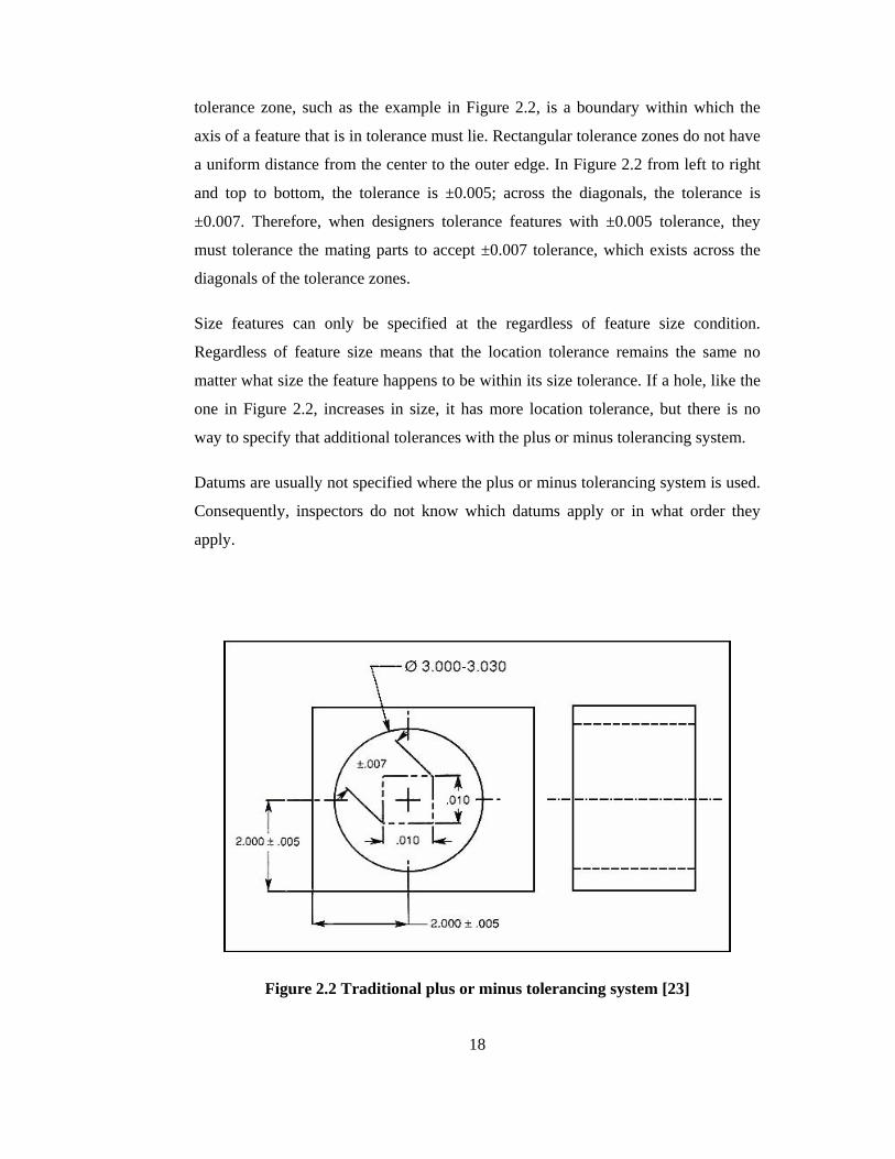
tolerance zone, such as the example in Figure 2.2, is a boundary within which the
axis of a feature that is in tolerance must lie. Rectangular tolerance zones do not have
a uniform distance from the center to the outer edge. In Figure 2.2 from left to right
and top to bottom, the tolerance is ±0.005; across the diagonals, the tolerance is
±0.007. Therefore, when designers tolerance features with ±0.005 tolerance, they
must tolerance the mating parts to accept ±0.007 tolerance, which exists across the
diagonals of the tolerance zones.
Size features can only be specified at the regardless of feature size condition.
Regardless of feature size means that the location tolerance remains the same no
matter what size the feature happens to be within its size tolerance. If a hole, like the
one in Figure 2.2, increases in size, it has more location tolerance, but there is no
way to specify that additional tolerances with the plus or minus tolerancing system.
Datums are usually not specified where the plus or minus tolerancing system is used.
Consequently, inspectors do not know which datums apply or in what order they
apply.
Figure 2.2 Traditional plus or minus tolerancing system [23]
19
2.4 Profile Tolerancing
A profile is the outline of an object. Specifically, the profile of a line is the outline of
an object in a plane as the plane passes through the object. The profile of a surface is
the result of projecting the profile of an object on a plane or taking cross sections
through the object at various intervals.
Profile tolerancing is a powerful and versatile tolerancing tool which can be used to
control just the size and shape of a feature or the size, shape, orientation, and location
of an irregular shaped feature. The profile tolerance controls the orientation and
location of features with unusual shapes.
Since acquiring desired geometrical accuracy and surface quality is quite important
on the surface profile of die cavities, profile tolerancing is frequently utilized in the
specifications of the die cavities.
A profile view or section view of a part is dimensioned with basic dimensions. A true
profile may be dimensioned with basic size dimensions, basic coordinate dimensions,
basic radii, basic angular dimensions, formulae. The feature control frame is always
directed to the profile surface with a leader. Profile is a surface control; the
association of a profile tolerance with an extension or a dimension line is
inappropriate. The profile feature control frame contains the profile of a line or of a
surface symbol and a tolerance. Since profile controls are surface controls,
cylindrical tolerance zones and material conditions do not apply in the tolerance
section of profile feature control frames. The shape of the tolerance is the shape of
the profile not a cylinder, and material condition modifiers do not apply to surface
controls.
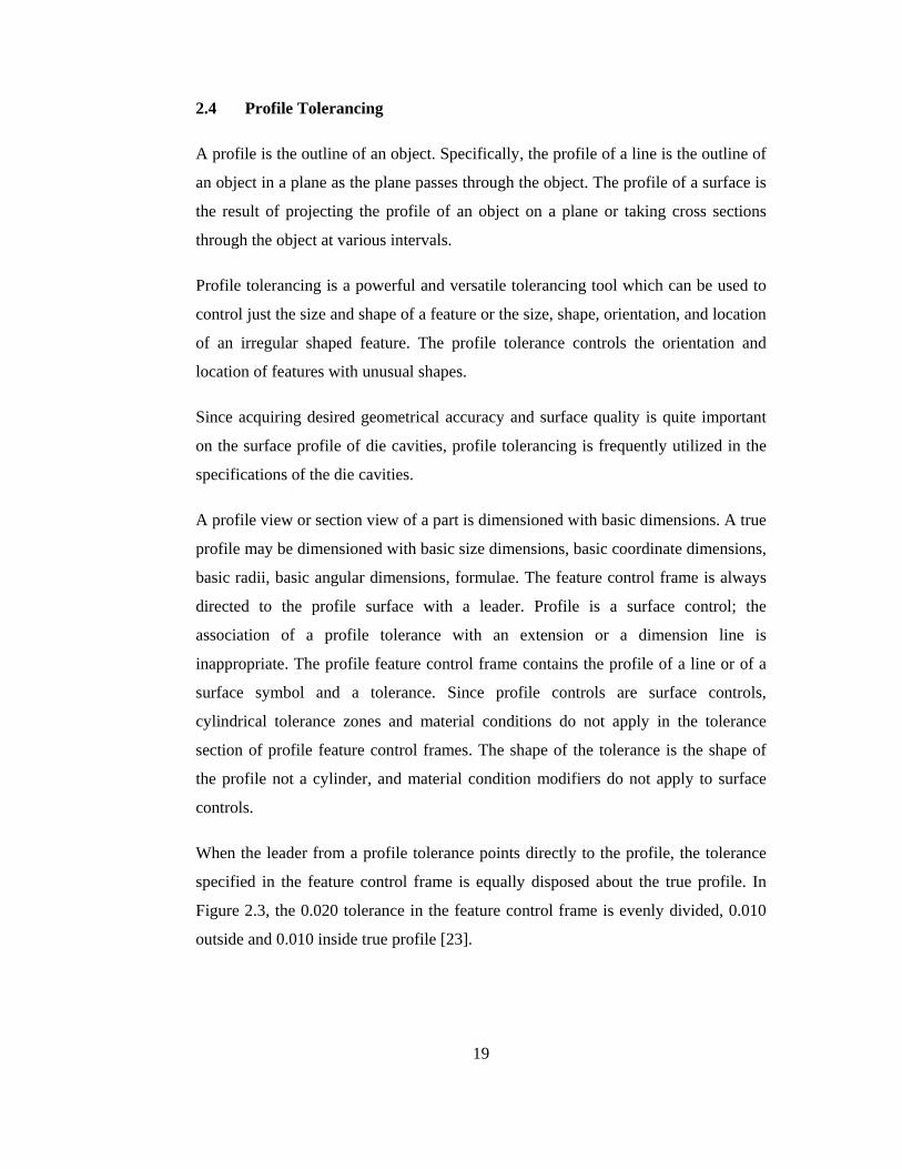
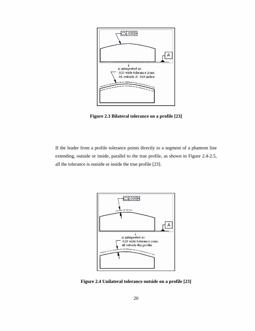
When the leader from a profile tolerance points directly to the profile, the tolerance
specified in the feature control frame is equally disposed about the true profile. In
Figure 2.3, the 0.020 tolerance in the feature control frame is evenly divided, 0.010
outside and 0.010 inside true profile [23].
20
Figure 2.3 Bilateral tolerance on a profile [23]
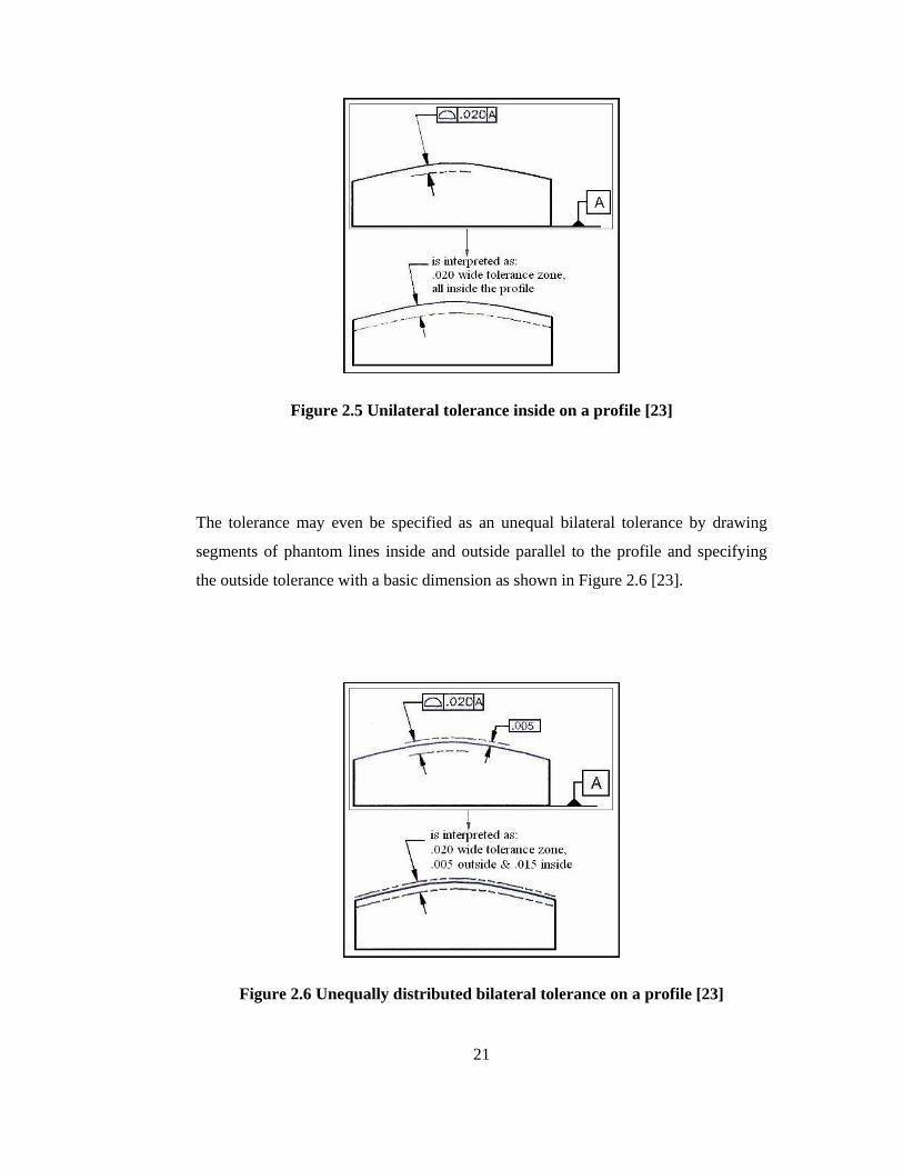
If the leader from a profile tolerance points directly to a segment of a phantom line
extending, outside or inside, parallel to the true profile, as shown in Figure 2.4-2.5,
all the tolerance is outside or inside the true profile [23].
Figure 2.4 Unilateral tolerance outside on a profile [23]
21
Figure 2.5 Unilateral tolerance inside on a profile [23]
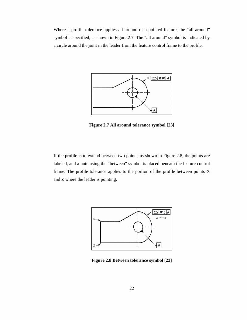
The tolerance may even be specified as an unequal bilateral tolerance by drawing
segments of phantom lines inside and outside parallel to the profile and specifying
the outside tolerance with a basic dimension as shown in Figure 2.6 [23].
Figure 2.6 Unequally distributed bilateral tolerance on a profile [23]
22
Where a profile tolerance applies all around of a pointed feature, the “all around”
symbol is specified, as shown in Figure 2.7. The “all around” symbol is indicated by
a circle around the joint in the leader from the feature control frame to the profile.
Figure 2.7 All around tolerance symbol [23]
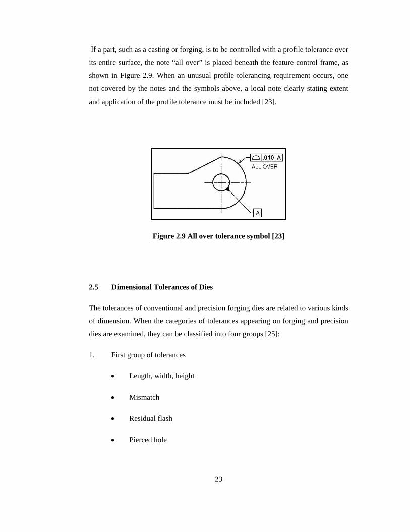
If the profile is to extend between two points, as shown in Figure 2.8, the points are
labeled, and a note using the “between” symbol is placed beneath the feature control
frame. The profile tolerance applies to the portion of the profile between points X
and Z where the leader is pointing.
Figure 2.8 Between tolerance symbol [23]
23
If a part, such as a casting or forging, is to be controlled with a profile tolerance over
its entire surface, the note “all over” is placed beneath the feature control frame, as
shown in Figure 2.9. When an unusual profile tolerancing requirement occurs, one
not covered by the notes and the symbols above, a local note clearly stating extent
and application of the profile tolerance must be included [23].
Figure 2.9 All over tolerance symbol [23]
2.5 Dimensional Tolerances of Dies
The tolerances of conventional and precision forging dies are related to various kinds
of dimension. When the categories of tolerances appearing on forging and precision
dies are examined, they can be classified into four groups [25]:
1. First group of tolerances
• Length, width, height
• Mismatch
• Residual flash
• Pierced hole
24
2. Second group of tolerances
• Thickness
• Ejector marks
3. Third group of tolerances
• Straightness and thickness
• Center to center dimensions
4. Other categories of tolerance
• Fillet and edge radii
• Burr
• Surface
• Draft angle surfaces
• Eccentricity for deep holes
• Deformation of sheared ends
• Deviation of form specified contour
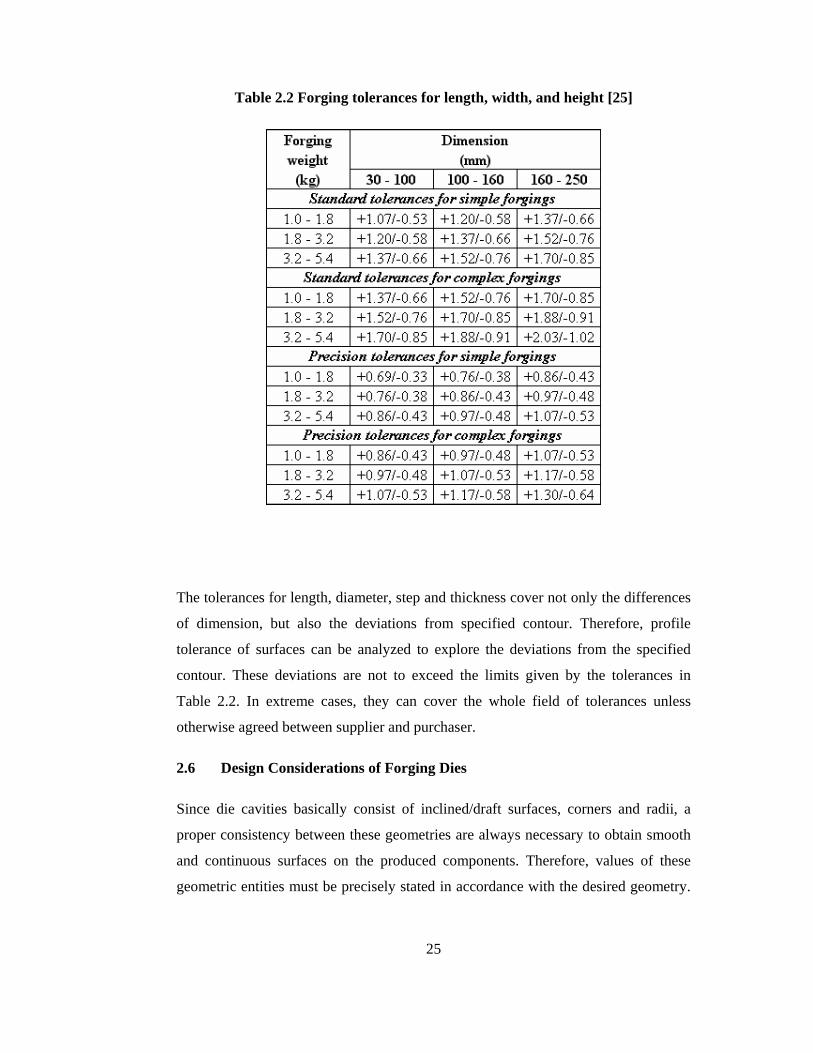
The German standard for forging tolerances, DIN 7526 [25] gives comprehensive
tolerance values for both normal and precision forgings. It is a well conceived
standard that takes into account the weight of a forging, its complexity, and the
difficulty of the material being forged. Table 2.2 illustrates the tolerances values
from that standard for both simple and complex forgings. The tolerances in this table
apply to dimensions of length, width, and height including diameters on one side of
the parting line. All variations, including those due to die wear, die sinking, and
shrinkage, are included in these tolerances [25].
25
Table 2.2 Forging tolerances for length, width, and height [25]
The tolerances for length, diameter, step and thickness cover not only the differences
of dimension, but also the deviations from specified contour. Therefore, profile
tolerance of surfaces can be analyzed to explore the deviations from the specified
contour. These deviations are not to exceed the limits given by the tolerances in
Table 2.2. In extreme cases, they can cover the whole field of tolerances unless
otherwise agreed between supplier and purchaser.
2.6 Design Considerations of Forging Dies
Since die cavities basically consist of inclined/draft surfaces, corners and radii, a
proper consistency between these geometries are always necessary to obtain smooth
and continuous surfaces on the produced components. Therefore, values of these
geometric entities must be precisely stated in accordance with the desired geometry.
26
Before determining the profile of the experimental study, design considerations of
forging die cavities and current applications in Aksan Steel Forging Company have
been investigated in detail.
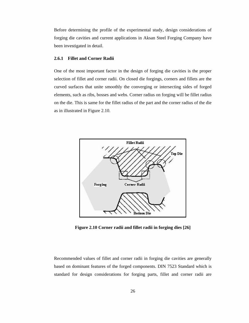
2.6.1 Fillet and Corner Radii
One of the most important factor in the design of forging die cavities is the proper
selection of fillet and corner radii. On closed die forgings, corners and fillets are the
curved surfaces that unite smoothly the converging or intersecting sides of forged
elements, such as ribs, bosses and webs. Corner radius on forging will be fillet radius
on the die. This is same for the fillet radius of the part and the corner radius of the die
as in illustrated in Figure 2.10.
Figure 2.10 Corner radii and fillet radii in forging dies [26]
Recommended values of fillet and corner radii in forging die cavities are generally
based on dominant features of the forged components. DIN 7523 Standard which is
standard for design considerations for forging parts, fillet and corner radii are
27
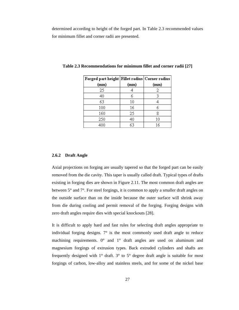
determined according to height of the forged part. In Table 2.3 recommended values
for minimum fillet and corner radii are presented.
Table 2.3 Recommendations for minimum fillet and corner radii [27]
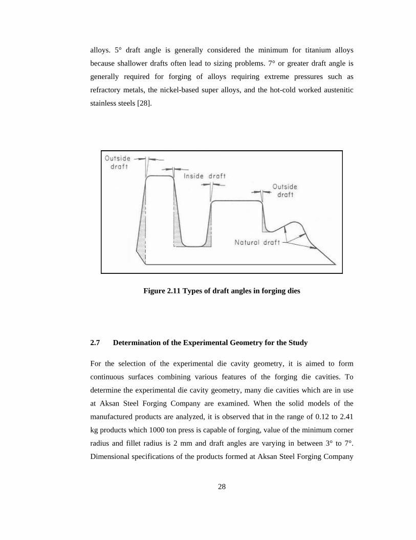
2.6.2 Draft Angle
Axial projections on forging are usually tapered so that the forged part can be easily
removed from the die cavity. This taper is usually called draft. Typical types of drafts
existing in forging dies are shown in Figure 2.11. The most common draft angles are
between 5° and 7°. For steel forgings, it is common to apply a smaller draft angles on
the outside surface than on the inside because the outer surface will shrink away
from die during cooling and permit removal of the forging. Forging designs with
zero draft angles require dies with special knockouts [28].
It is difficult to apply hard and fast rules for selecting draft angles appropriate to
individual forging designs. 7° is the most commonly used draft angle to reduce
machining requirements. 0° and 1° draft angles are used on aluminum and
magnesium forgings of extrusion types. Back extruded cylinders and shafts are
frequently designed with 1° draft. 3° to 5° degree draft angle is suitable for most
forgings of carbon, low-alloy and stainless steels, and for some of the nickel base
28
alloys. 5° draft angle is generally considered the minimum for titanium alloys
because shallower drafts often lead to sizing problems. 7° or greater draft angle is
generally required for forging of alloys requiring extreme pressures such as
refractory metals, the nickel-based super alloys, and the hot-cold worked austenitic
stainless steels [28].
Figure 2.11 Types of draft angles in forging dies
2.7 Determination of the Experimental Geometry for the Study
For the selection of the experimental die cavity geometry, it is aimed to form
continuous surfaces combining various features of the forging die cavities. To
determine the experimental die cavity geometry, many die cavities which are in use
at Aksan Steel Forging Company are examined. When the solid models of the
manufactured products are analyzed, it is observed that in the range of 0.12 to 2.41
kg products which 1000 ton press is capable of forging, value of the minimum corner
radius and fillet radius is 2 mm and draft angles are varying in between 3° to 7°.
Dimensional specifications of the products formed at Aksan Steel Forging Company
29
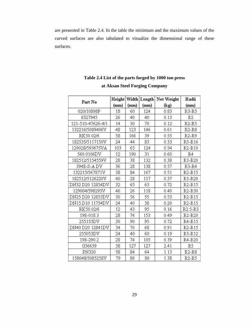
are presented in Table 2.4. In the table the minimum and the maximum values of the
curved surfaces are also tabulated to visualize the dimensional range of these
surfaces.
Table 2.4 List of the parts forged by 1000 ton press
at Aksan Steel Forging Company
30
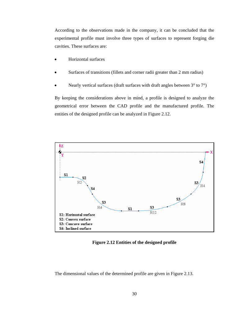
According to the observations made in the company, it can be concluded that the
experimental profile must involve three types of surfaces to represent forging die
cavities. These surfaces are:
• Horizontal surfaces
• Surfaces of transitions (fillets and corner radii greater than 2 mm radius)
• Nearly vertical surfaces (draft surfaces with draft angles between 3° to 7°)
By keeping the considerations above in mind, a profile is designed to analyze the
geometrical error between the CAD profile and the manufactured profile. The
entities of the designed profile can be analyzed in Figure 2.12.
Figure 2.12 Entities of the designed profile
The dimensional values of the determined profile are given in Figure 2.13.
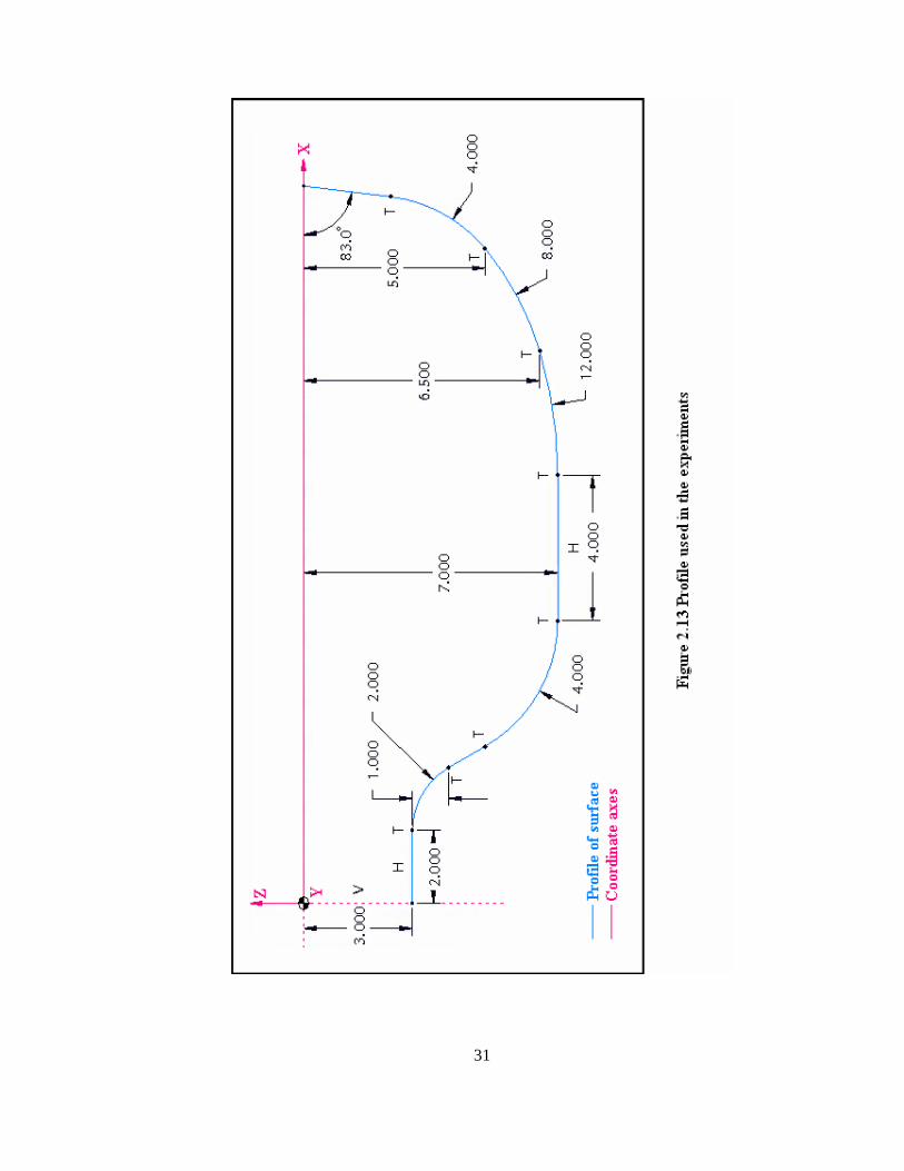
31
32
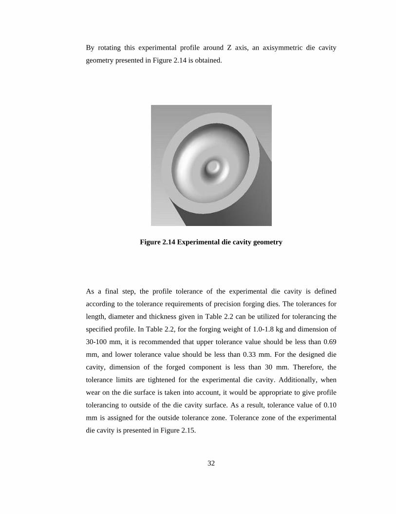
By rotating this experimental profile around Z axis, an axisymmetric die cavity
geometry presented in Figure 2.14 is obtained.
Figure 2.14 Experimental die cavity geometry
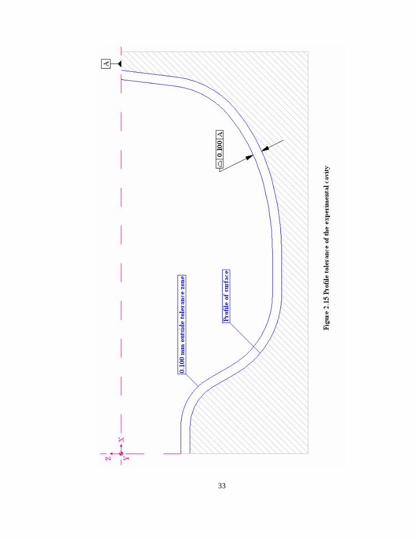
As a final step, the profile tolerance of the experimental die cavity is defined
according to the tolerance requirements of precision forging dies. The tolerances for
length, diameter and thickness given in Table 2.2 can be utilized for tolerancing the
specified profile. In Table 2.2, for the forging weight of 1.0-1.8 kg and dimension of
30-100 mm, it is recommended that upper tolerance value should be less than 0.69
mm, and lower tolerance value should be less than 0.33 mm. For the designed die
cavity, dimension of the forged component is less than 30 mm. Therefore, the
tolerance limits are tightened for the experimental die cavity. Additionally, when
wear on the die surface is taken into account, it would be appropriate to give profile
tolerancing to outside of the die cavity surface. As a result, tolerance value of 0.10
mm is assigned for the outside tolerance zone. Tolerance zone of the experimental
die cavity is presented in Figure 2.15.
33
34
CHAPTER 3
ROUGH CUT MILLING OF EXPERIMENTAL DIE CAVITIES
In this chapter, details of rough cut milling have been presented and cutting strategies
for the experimental die cavity have been analyzed. Feed rate optimization has been
performed to satisfy constant metal removal rate along the tool path trajectory.
Finally, optimized rough cut milling codes have been implemented to the die cavities
which are required for the finish cut experiments.
3.1 Importance of Rough Cutting Operations in Forging Die Manufacturing
Nowadays, current trend in forging die manufacturing is to produce high quality
surface with an accurate geometrical properties using high speed machining centers.
With the introduction of new developments in CNC milling technology, higher feed
rates and cutting speeds are more and more applicable. Advances in feed rate and
cutting speed provide great reductions in the production time of forging die cavities.
However, obtaining geometrical accuracy in accordance with the product
specifications is still primary objective; therefore, the most suitable cutting
parameters for each operation must be carefully selected.
Many researchers pay attention to optimizing finish parameters of the cutting
operations but this is not completely sufficient to increase the efficiency of
manufacturing processes of dies. As expected, a rough cutting operation is performed
before each finishing operation. For this reason, proper strategies must be defined
and applied for both rough cutting and finish cutting operations. A well done rough
cutting operation not only provides a smoother surface before finish cutting but also
increases tool life considerably.
35
In terms of rough machining of die cavities, the principal goals of the operation
should be:
• Removing the same amount of material with the minimum cycle time
• Reducing number of plunge and retract motions of the tool
• Obtaining the minimum tool path length for the removal of the same amount
of volume
• Providing a continuous contact of tool-workpiece to decrease the fluctuations
of temperature on the cutting edge
• Decreasing nonproductive time
3.2 Cutting Parameters for Rough Machining
There are many parameters influencing the characteristics of milling process.
However, when the cutting parameters are considered, main parameters can be
classified as:
• Axial depth of cut (ap) [mm]
• Radial depth of cut (ae) [mm]
• Feed rate (Vf) [mm/min]
• Cutting speed (Vc) [m/min]
• Type of milling i.e. down or up milling
Axial depth of cut is the axial engagement of the tool with respect to workpiece.
Proper value of axial depth of cut should be determined to prevent excessive tool tip
failure.
Radial depth of cut or radial engagement of the tool is also known as step over. For
the milling process, maximizing metal removal rate is the basic goal in rough cutting
36
operations. Therefore, it should be logical to use 100% radial engagement of the
cutting tool. However, choosing that amount of engagement substantially decreases
tool life and tool performance. It would be better in terms of tool life and
performance to use 66% radial engagement of the tool as a step over value [29].
As cutting tools are varying in terms of number of teeth on the tool tip, feed rate can
be related with number of cutting flutes, spindle speed and feed per tooth according
to the following equation:
NnfV ttf ⋅⋅= (3.1)
where ft is feed in mm per tooth, nt is number of cutting flutes on the tool, N is
spindle speed in rpm.
Cutting speed is the speed difference between cutting tool and surface of the
workpiece it is operating on. It depends on tool diameter and spindle speed; and can
be calculated according to the following equation:
1000
NDVc⋅⋅
=π (3.2)
where D is tool diameter in mm, N is spindle speed in rpm.
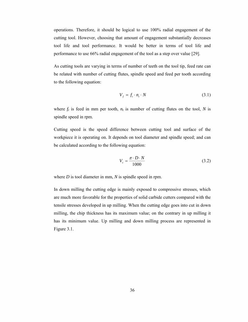
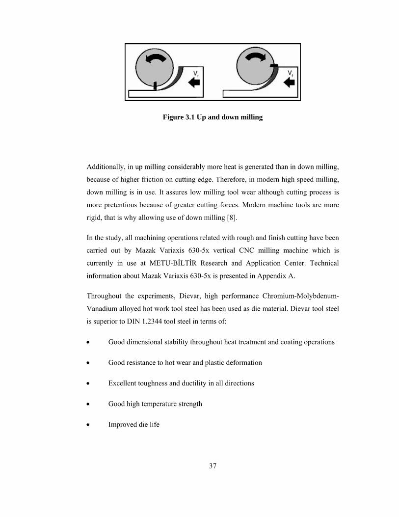
In down milling the cutting edge is mainly exposed to compressive stresses, which
are much more favorable for the properties of solid carbide cutters compared with the
tensile stresses developed in up milling. When the cutting edge goes into cut in down
milling, the chip thickness has its maximum value; on the contrary in up milling it
has its minimum value. Up milling and down milling process are represented in
Figure 3.1.
37
Figure 3.1 Up and down milling
Additionally, in up milling considerably more heat is generated than in down milling,
because of higher friction on cutting edge. Therefore, in modern high speed milling,
down milling is in use. It assures low milling tool wear although cutting process is
more pretentious because of greater cutting forces. Modern machine tools are more
rigid, that is why allowing use of down milling [8].
In the study, all machining operations related with rough and finish cutting have been
carried out by Mazak Variaxis 630-5x vertical CNC milling machine which is
currently in use at METU-BİLTİR Research and Application Center. Technical
information about Mazak Variaxis 630-5x is presented in Appendix A.
Throughout the experiments, Dievar, high performance Chromium-Molybdenum-
Vanadium alloyed hot work tool steel has been used as die material. Dievar tool steel
is superior to DIN 1.2344 tool steel in terms of:
• Good dimensional stability throughout heat treatment and coating operations
• Good resistance to hot wear and plastic deformation
• Excellent toughness and ductility in all directions
• Good high temperature strength
• Improved die life
38
• Excellent hardenability
Properties of Dievar tool steel are given in Appendix B.
As rough cutting tool, Ø6 mm solid carbide end mill with two flutes is selected.
Cutting speed and feed recommendations of the tool steel manufacturer and
properties of the selected tool are presented in Appendix C.
In order to minimize vibrations of the tool, AA class collet has been used to mount
cutters to HSK R32 tool holders [30].
Finally, throughout the experiments flood cooling has been applied to counteract
excessive heat generation at the cutting edges of the tool.
3.3 Constant Metal Removal Rate in Rough Cut
In the milling process, material removal rate is defined as the rate at which material
is removed from an unfinished part, usually measured in cubic millimeters per
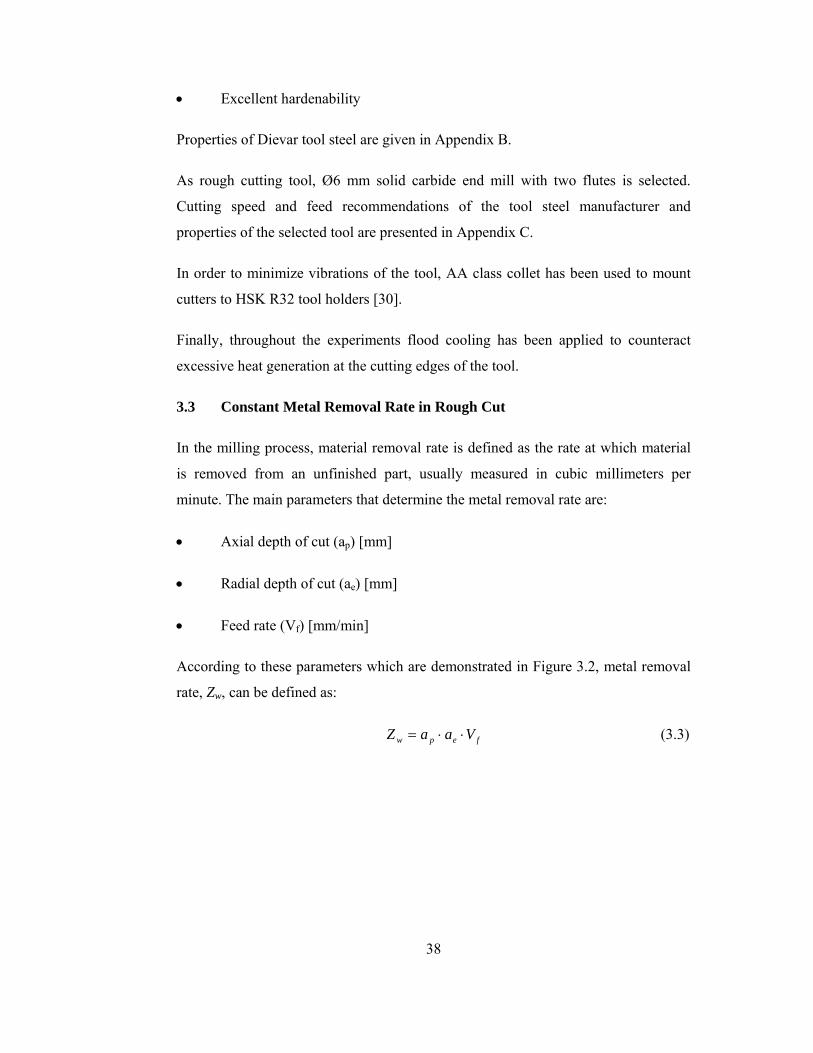
minute. The main parameters that determine the metal removal rate are:
• Axial depth of cut (ap) [mm]
• Radial depth of cut (ae) [mm]
• Feed rate (Vf) [mm/min]
According to these parameters which are demonstrated in Figure 3.2, metal removal
rate, Zw, can be defined as:
fepw VaaZ ⋅⋅= (3.3)
39
Figure 3.2 Parameters of metal removal rate
Maintaining a constant metal removal rate keeps the cutter at its maximum possible
rate of advance into material for the varying cutting conditions. However, to keep
material removal rate constant during any kind of operation, either radial depth of cut
and feed rate must be kept constant or multiplication term of radial depth of cut and
feed rate must be kept constant. Determining the exact and optimum feed rate
selection for sculptured surface is very difficult and requires experience. By selecting
a fixed feed rate based upon the maximum force, which is obtained during full length
of machining, the tool is saved but it results in extra machining time, which reduces
productivity. By optimizing the feed rate, both the objectives of saving the tool (more
tool life) and also reducing machining time thereby increasing productivity can be
achieved. Since rough machining operations are strongly geometrical feature
dependent, feed rate adjustments are usually essential to maintain constant metal
removal rate.
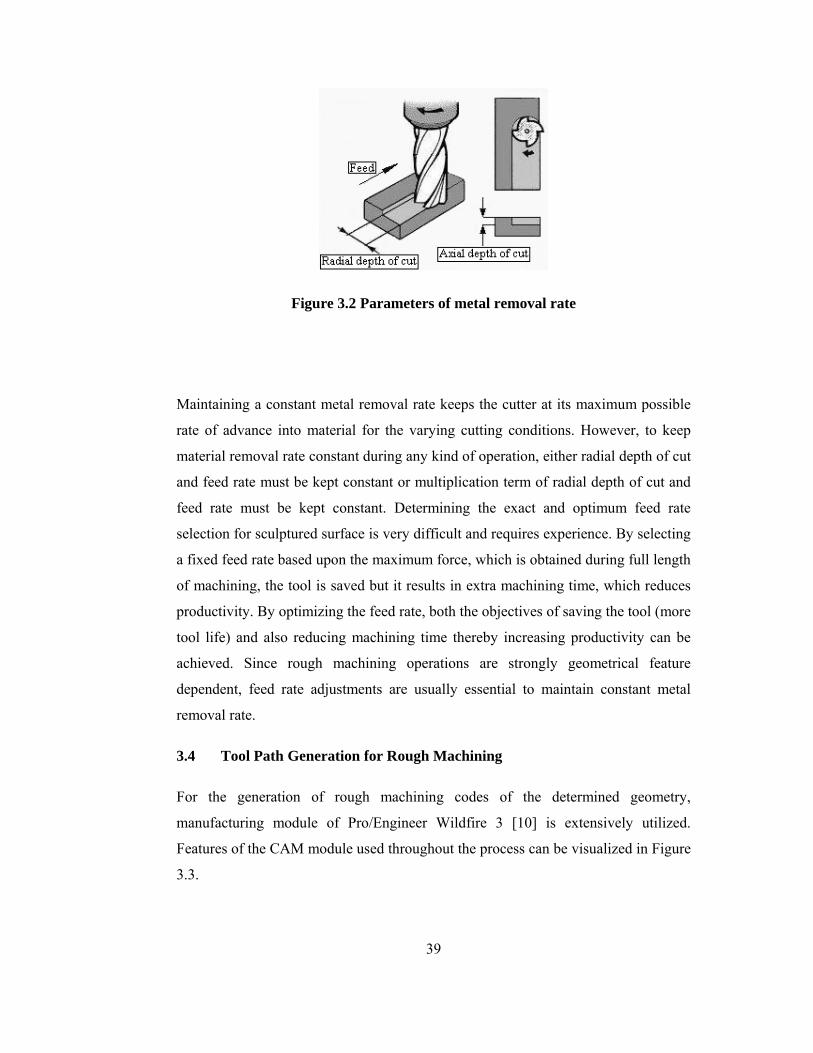
3.4 Tool Path Generation for Rough Machining
For the generation of rough machining codes of the determined geometry,
manufacturing module of Pro/Engineer Wildfire 3 [10] is extensively utilized.
Features of the CAM module used throughout the process can be visualized in Figure
3.3.
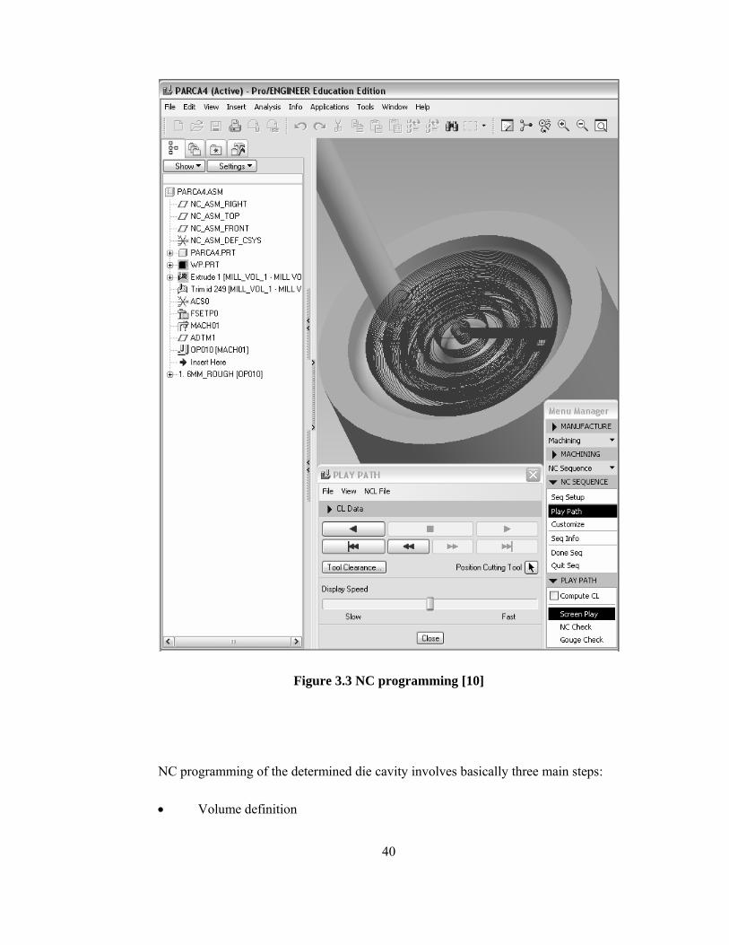
40
Figure 3.3 NC programming [10]
NC programming of the determined die cavity involves basically three main steps:
• Volume definition
41
• Cutting parameter selection
• Code generation
Initially, excess volume that is intended to be removed from the die cavity is defined.
After that, tool and cutting parameters are determined by considering the cavity
geometry. Cutter location data for the operation is then formed by taking the
predefined cutting parameters and the tool data into consideration. This data file is
then post processed and checked by NC simulation package of Pro/Engineer Wildfire
3 [10] whether code is collision free or not. Finally, transformed G-code file is fed to
the CNC unit of Mazak Variaxis 630-5x.
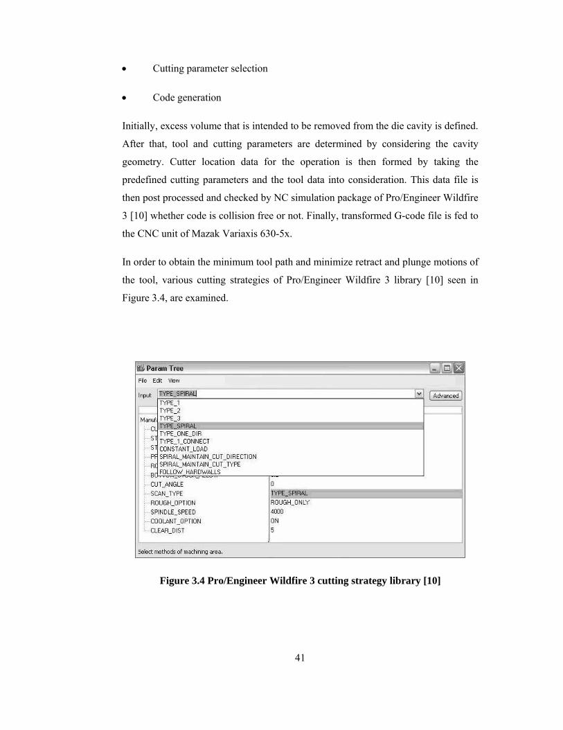
In order to obtain the minimum tool path and minimize retract and plunge motions of
the tool, various cutting strategies of Pro/Engineer Wildfire 3 library [10] seen in
Figure 3.4, are examined.
Figure 3.4 Pro/Engineer Wildfire 3 cutting strategy library [10]
42
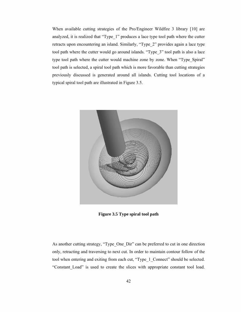
When available cutting strategies of the Pro/Engineer Wildfire 3 library [10] are
analyzed, it is realized that “Type_1” produces a lace type tool path where the cutter
retracts upon encountering an island. Similarly, “Type_2” provides again a lace type
tool path where the cutter would go around islands. “Type_3” tool path is also a lace
type tool path where the cutter would machine zone by zone. When “Type_Spiral”
tool path is selected, a spiral tool path which is more favorable than cutting strategies
previously discussed is generated around all islands. Cutting tool locations of a
typical spiral tool path are illustrated in Figure 3.5.
Figure 3.5 Type spiral tool path
As another cutting strategy, “Type_One_Dir” can be preferred to cut in one direction
only, retracting and traversing to next cut. In order to maintain contour follow of the
tool when entering and exiting from each cut, “Type_1_Connect” should be selected.
“Constant_Load” is used to create the slices with appropriate constant tool load.
43
However, in this approach radial depth of cut i.e. step over value is limited to half of
the tool diameter which is undesirable. “Spiral_Maintain_Cut_Direction” enables a
spiral tool path maintaining cut direction and “Spiral_Maintain_Cut_Type” enables
spiral tool path maintaining cut type but again the radial depth of cut values are
limited to half of tool diameter which is unacceptable. Finally in
“Follow_Hardwalls” each cut would follow hard walls of the feature.
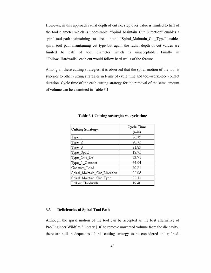
Among all these cutting strategies, it is observed that the spiral motion of the tool is
superior to other cutting strategies in terms of cycle time and tool-workpiece contact
duration. Cycle time of the each cutting strategy for the removal of the same amount
of volume can be examined in Table 3.1.
Table 3.1 Cutting strategies vs. cycle time
3.5 Deficiencies of Spiral Tool Path
Although the spiral motion of the tool can be accepted as the best alternative of
Pro/Engineer Wildfire 3 library [10] to remove unwanted volume from the die cavity,
there are still inadequacies of this cutting strategy to be considered and refined.
44
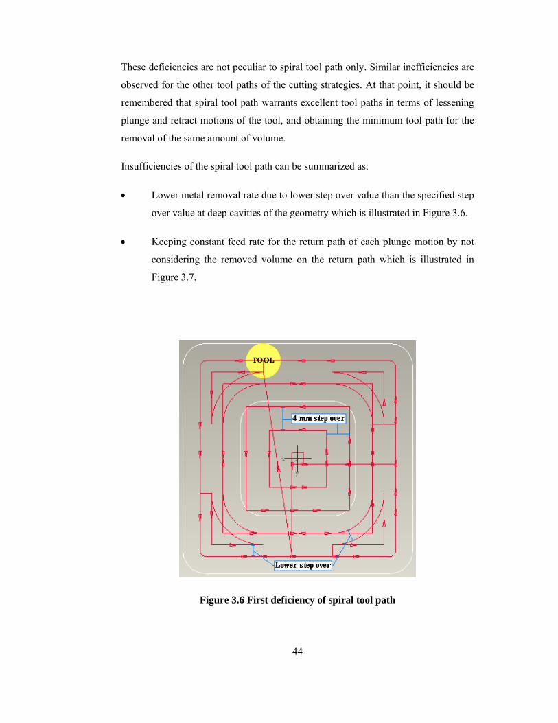
These deficiencies are not peculiar to spiral tool path only. Similar inefficiencies are
observed for the other tool paths of the cutting strategies. At that point, it should be
remembered that spiral tool path warrants excellent tool paths in terms of lessening
plunge and retract motions of the tool, and obtaining the minimum tool path for the
removal of the same amount of volume.
Insufficiencies of the spiral tool path can be summarized as:
• Lower metal removal rate due to lower step over value than the specified step
over value at deep cavities of the geometry which is illustrated in Figure 3.6.
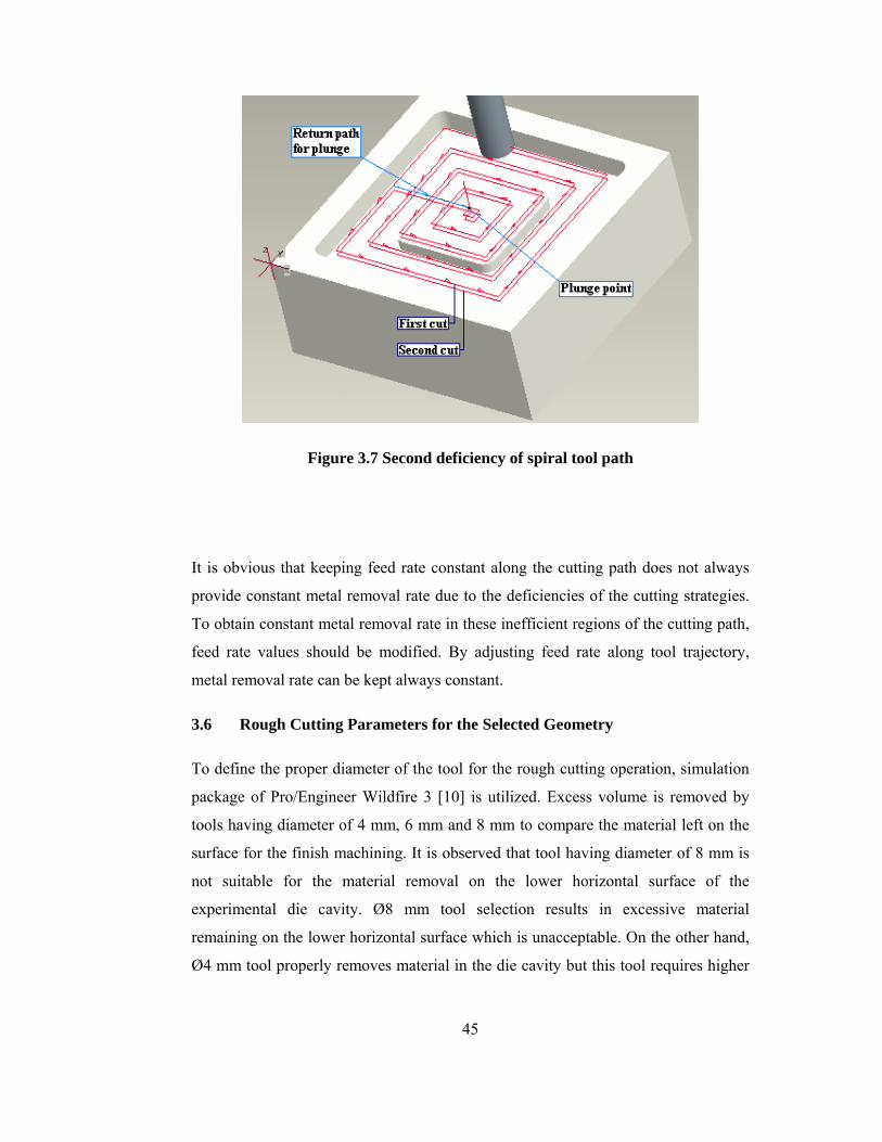
• Keeping constant feed rate for the return path of each plunge motion by not
considering the removed volume on the return path which is illustrated in
Figure 3.7.
Figure 3.6 First deficiency of spiral tool path
45
Figure 3.7 Second deficiency of spiral tool path
It is obvious that keeping feed rate constant along the cutting path does not always
provide constant metal removal rate due to the deficiencies of the cutting strategies.
To obtain constant metal removal rate in these inefficient regions of the cutting path,
feed rate values should be modified. By adjusting feed rate along tool trajectory,
metal removal rate can be kept always constant.
3.6 Rough Cutting Parameters for the Selected Geometry
To define the proper diameter of the tool for the rough cutting operation, simulation
package of Pro/Engineer Wildfire 3 [10] is utilized. Excess volume is removed by
tools having diameter of 4 mm, 6 mm and 8 mm to compare the material left on the
surface for the finish machining. It is observed that tool having diameter of 8 mm is
not suitable for the material removal on the lower horizontal surface of the
experimental die cavity. Ø8 mm tool selection results in excessive material
remaining on the lower horizontal surface which is unacceptable. On the other hand,
Ø4 mm tool properly removes material in the die cavity but this tool requires higher
46
production time when it is compared with Ø6 mm tool. According to these analyses,
it is realized that Ø6 mm tool not only removes the excess volume efficiently but also
provides a reasonable production time. Therefore, Ø6 mm solid carbide end mill with
two cutting flutes is chosen for the rough cutting operations.
For the determination of the axial depth of cut value, tool properties and depth of cut
value for the finishing operation are taken into consideration. Surfaces having
staircase shape are generally obtained on the curved regions of the die cavities after
rough cutting process. The height of these stairs can be minimized by selecting low
axial depth of cut values for the rough cutting operations. However, taking a low
axial depth of cut value definitely results in higher production time. Therefore, by
keeping these considerations in mind, 0.2 mm is determined for the value of axial
depth of cut.
Radial depth of cut or step over value is defined as 4.0 mm. For the Ø6 mm solid
carbide end mill, step over value higher than 4.0 mm can be selected but this may
yield substantial decrease in tool life and performance. Therefore, 66% radial
engagement of the tool as step over value is utilized for the rough cutting operation
[29].
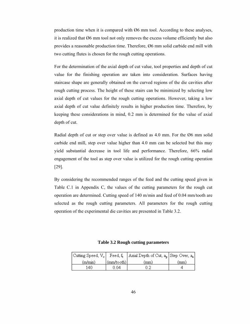
By considering the recommended ranges of the feed and the cutting speed given in
Table C.1 in Appendix C, the values of the cutting parameters for the rough cut
operation are determined. Cutting speed of 140 m/min and feed of 0.04 mm/tooth are
selected as the rough cutting parameters. All parameters for the rough cutting
operation of the experimental die cavities are presented in Table 3.2.
Table 3.2 Rough cutting parameters
47
Feed in mm per tooth value given in Table 3.2 can be converted to mm/min by using
Equations 3.1-3.2 respectively. For the Ø6 mm tool with cutting speed (Vc) of 140
m/min, spindle speed (N) is calculated as 7427 rpm. By multiplying this spindle
speed value with the number of cutting flutes (nt = 2) and feed (ft) of 0.04 mm/tooth,
feed rate (Vf) can be found as 594 mm/min.
3.7 Rough Cut Optimization
Due to the deficiencies mentioned in Section 3.5, rough machining codes of the
experimental die cavity are subjected to feed rate optimization to achieve substantial
amount of cycle time reduction. Optimized codes are generated for the rough
machining process by revising the feed rates along the cutting trajectory to maintain
constant metal removal rate. In the performed optimization, the programmed tool
path is not altered. Instead, optimization ensures that the tool path has the optimum
feed rate values to produce high quality parts in the least amount of time.
In the optimized tool path, these common inefficiencies of the original tool path are
eliminated:
• Excessively conservative feed rates
• Cutting feed rate used for motions in air
• No feed rate compensation for milling less (or more) material than expected
• No feed rate compensation for changing cutting conditions, such as: changing
axial and radial depth of cut
In the optimization process, original code is initially examined to find out the regions
where metal removal rate is lower than the predefined value. Predefined metal
removal rate can be computed by Equation 3.3. By multiplying axial depth of cut (ap)
of 0.2 mm with step over (ae) of 4.0 mm and feed rate (Vf) of 594 mm/min, metal
removal rate can be found as 475.2 mm3/min.
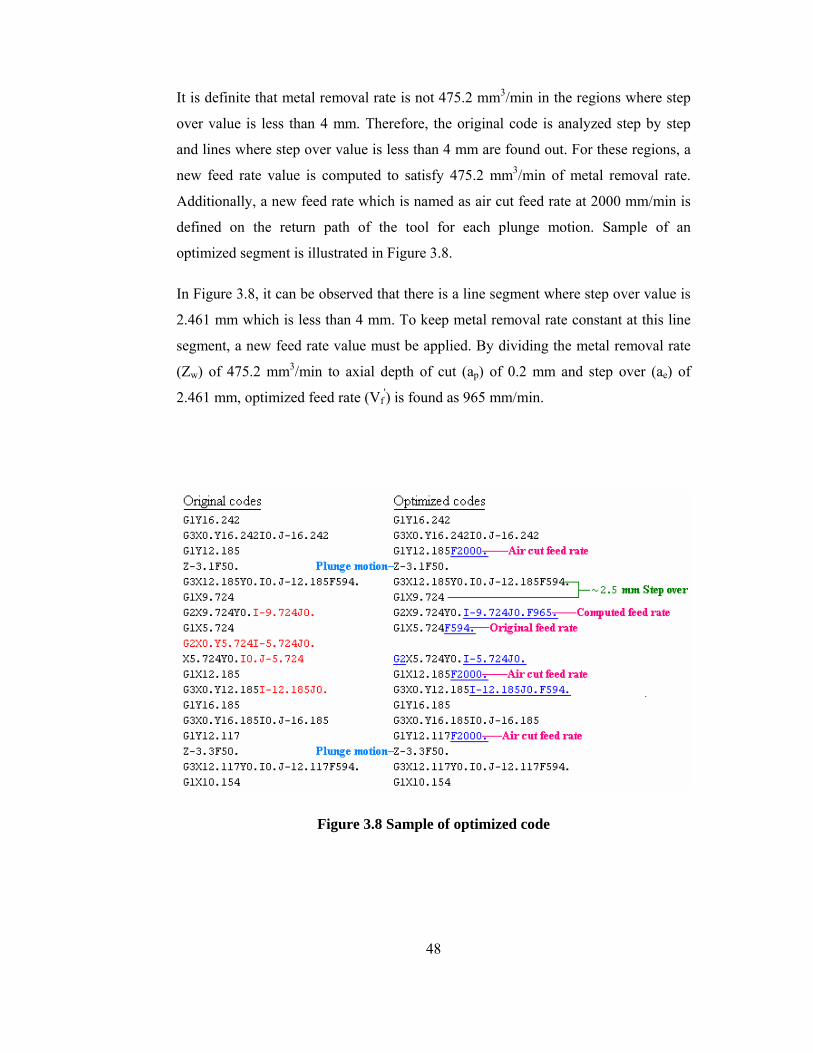
48
It is definite that metal removal rate is not 475.2 mm3/min in the regions where step
over value is less than 4 mm. Therefore, the original code is analyzed step by step
and lines where step over value is less than 4 mm are found out. For these regions, a
new feed rate value is computed to satisfy 475.2 mm3/min of metal removal rate.
Additionally, a new feed rate which is named as air cut feed rate at 2000 mm/min is
defined on the return path of the tool for each plunge motion. Sample of an
optimized segment is illustrated in Figure 3.8.
In Figure 3.8, it can be observed that there is a line segment where step over value is
2.461 mm which is less than 4 mm. To keep metal removal rate constant at this line
segment, a new feed rate value must be applied. By dividing the metal removal rate
(Zw) of 475.2 mm3/min to axial depth of cut (ap) of 0.2 mm and step over (ae) of
2.461 mm, optimized feed rate (Vf') is found as 965 mm/min.
Figure 3.8 Sample of optimized code
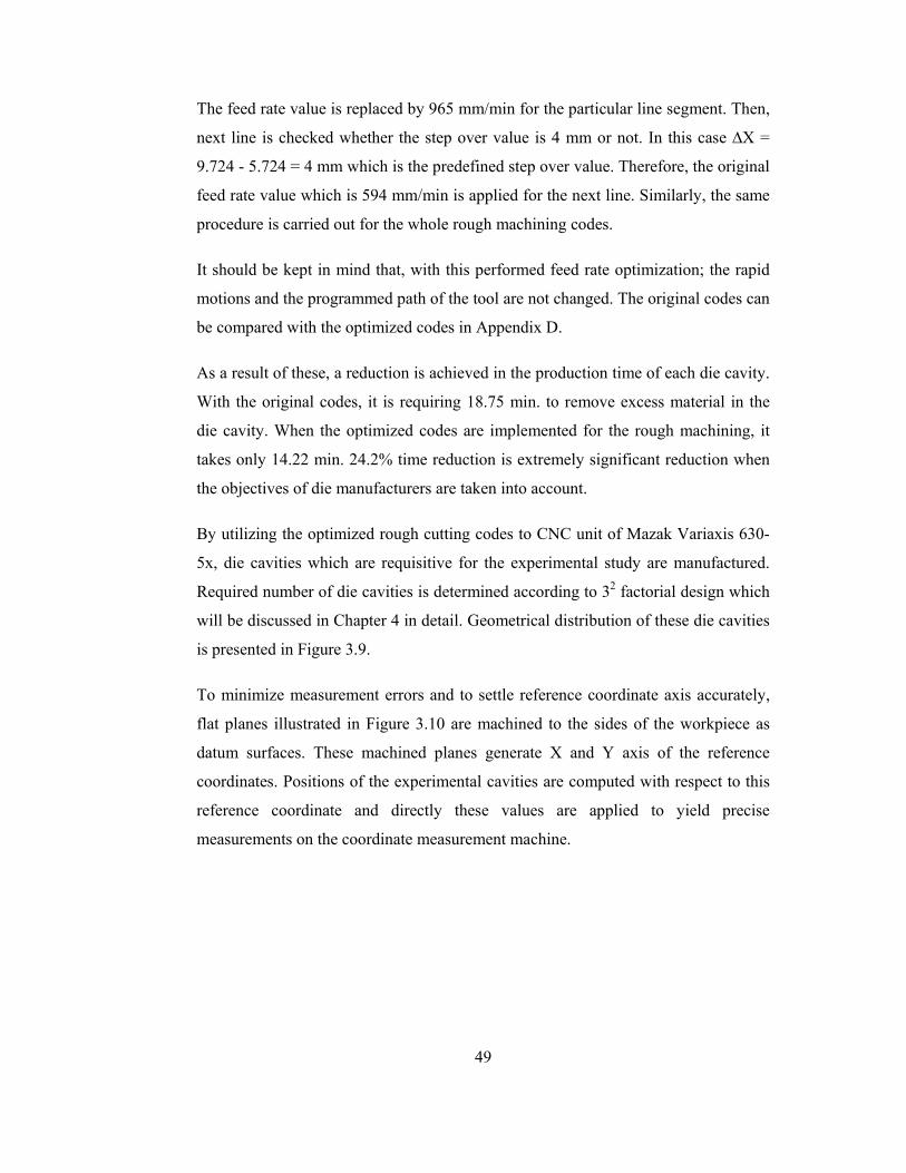
49
The feed rate value is replaced by 965 mm/min for the particular line segment. Then,
next line is checked whether the step over value is 4 mm or not. In this case ∆X =
9.724 - 5.724 = 4 mm which is the predefined step over value. Therefore, the original
feed rate value which is 594 mm/min is applied for the next line. Similarly, the same
procedure is carried out for the whole rough machining codes.
It should be kept in mind that, with this performed feed rate optimization; the rapid
motions and the programmed path of the tool are not changed. The original codes can
be compared with the optimized codes in Appendix D.
As a result of these, a reduction is achieved in the production time of each die cavity.
With the original codes, it is requiring 18.75 min. to remove excess material in the
die cavity. When the optimized codes are implemented for the rough machining, it
takes only 14.22 min. 24.2% time reduction is extremely significant reduction when
the objectives of die manufacturers are taken into account.
By utilizing the optimized rough cutting codes to CNC unit of Mazak Variaxis 630-
5x, die cavities which are requisitive for the experimental study are manufactured.
Required number of die cavities is determined according to 32 factorial design which
will be discussed in Chapter 4 in detail. Geometrical distribution of these die cavities
is presented in Figure 3.9.
To minimize measurement errors and to settle reference coordinate axis accurately,
flat planes illustrated in Figure 3.10 are machined to the sides of the workpiece as
datum surfaces. These machined planes generate X and Y axis of the reference
coordinates. Positions of the experimental cavities are computed with respect to this
reference coordinate and directly these values are applied to yield precise
measurements on the coordinate measurement machine.
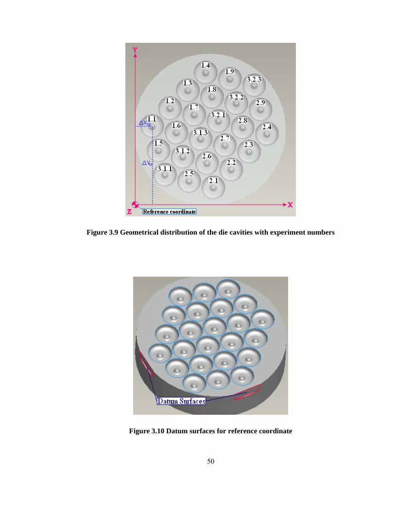
50
Figure 3.9 Geometrical distribution of the die cavities with experiment numbers
Figure 3.10 Datum surfaces for reference coordinate
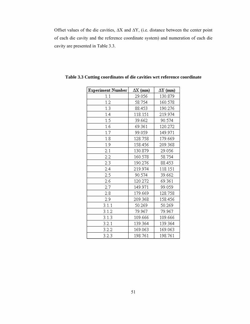
51
Offset values of the die cavities, ∆X and ∆Y, (i.e. distance between the center point
of each die cavity and the reference coordinate system) and numeration of each die
cavity are presented in Table 3.3.
Table 3.3 Cutting coordinates of die cavities wrt reference coordinate

52
CHAPTER 4
FINISH CUT MILLING OF EXPERIMENTAL DIE CAVITIES
In this chapter, three level factorial design for the experimental study has been
initially defined. Then, details of the finish cut parameter selection and experimental
levels are presented. Finally, geometrical error measurement technique for the
manufactured experimental cavity profile has been explained.
4.1 Three Level Factorial Design
3k design is a factorial design, that is, a factorial arrangement with k factors each at
three levels. Three levels of the factors are referred as low, intermediate, and high.
Each treatment in the 3k design are denoted by k digits, where the first digit indicates
the level of factor A, the second digit indicates the level of factor B and the kth digit
indicates the level of factor k. Geometry of 32 design is shown in Figure 4.1.
Figure 4.1 Treatment combinations in 32 design
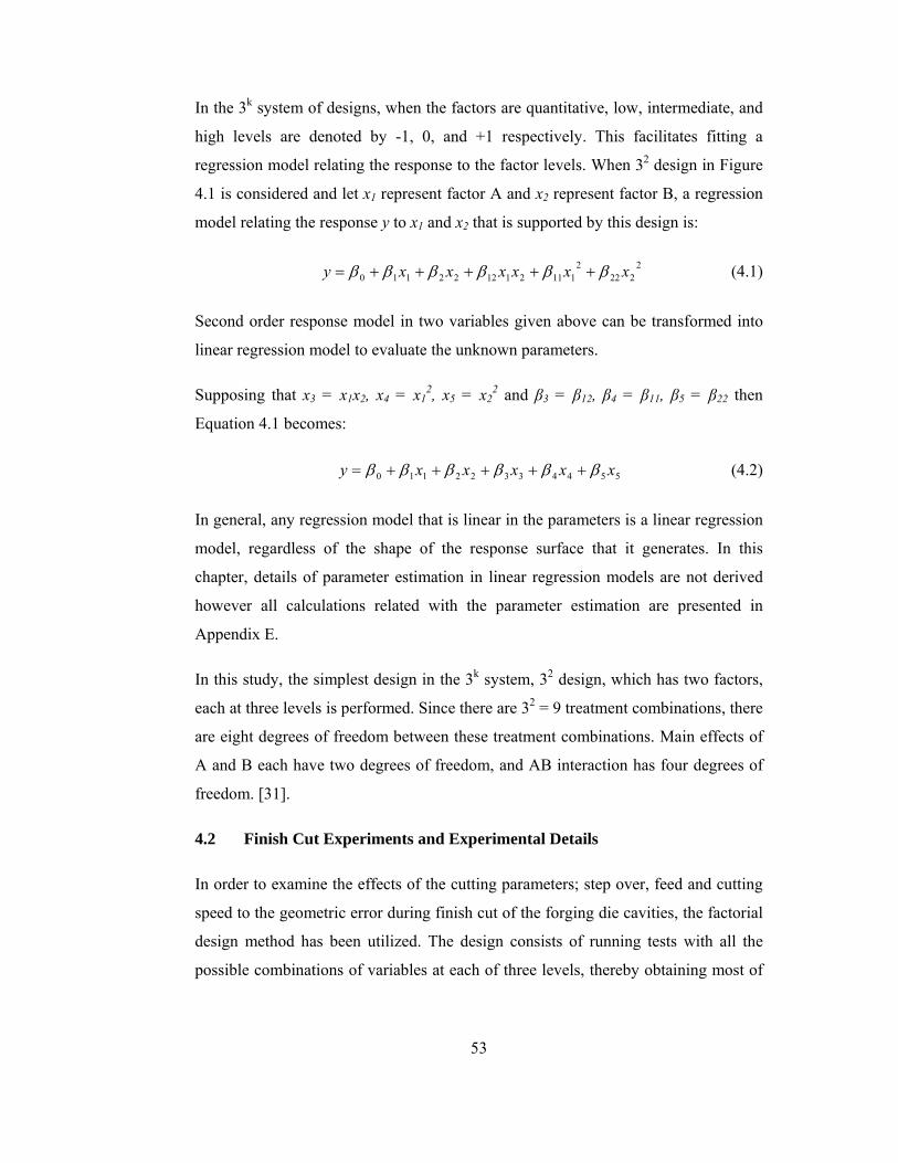
53
In the 3k system of designs, when the factors are quantitative, low, intermediate, and
high levels are denoted by -1, 0, and +1 respectively. This facilitates fitting a
regression model relating the response to the factor levels. When 32 design in Figure
4.1 is considered and let x1 represent factor A and x2 represent factor B, a regression
model relating the response y to x1 and x2 that is supported by this design is:
2222
2111211222110 xxxxxxy ββββββ +++++= (4.1)
Second order response model in two variables given above can be transformed into
linear regression model to evaluate the unknown parameters.
Supposing that x3 = x1x2, x4 = x12, x5 = x2
2 and β3 = β12, β4 = β11, β5 = β22 then
Equation 4.1 becomes:
55443322110 xxxxxy ββββββ +++++= (4.2)
In general, any regression model that is linear in the parameters is a linear regression
model, regardless of the shape of the response surface that it generates. In this
chapter, details of parameter estimation in linear regression models are not derived
however all calculations related with the parameter estimation are presented in
Appendix E.
In this study, the simplest design in the 3k system, 32 design, which has two factors,
each at three levels is performed. Since there are 32 = 9 treatment combinations, there
are eight degrees of freedom between these treatment combinations. Main effects of
A and B each have two degrees of freedom, and AB interaction has four degrees of
freedom. [31].
4.2 Finish Cut Experiments and Experimental Details
In order to examine the effects of the cutting parameters; step over, feed and cutting
speed to the geometric error during finish cut of the forging die cavities, the factorial
design method has been utilized. The design consists of running tests with all the
possible combinations of variables at each of three levels, thereby obtaining most of
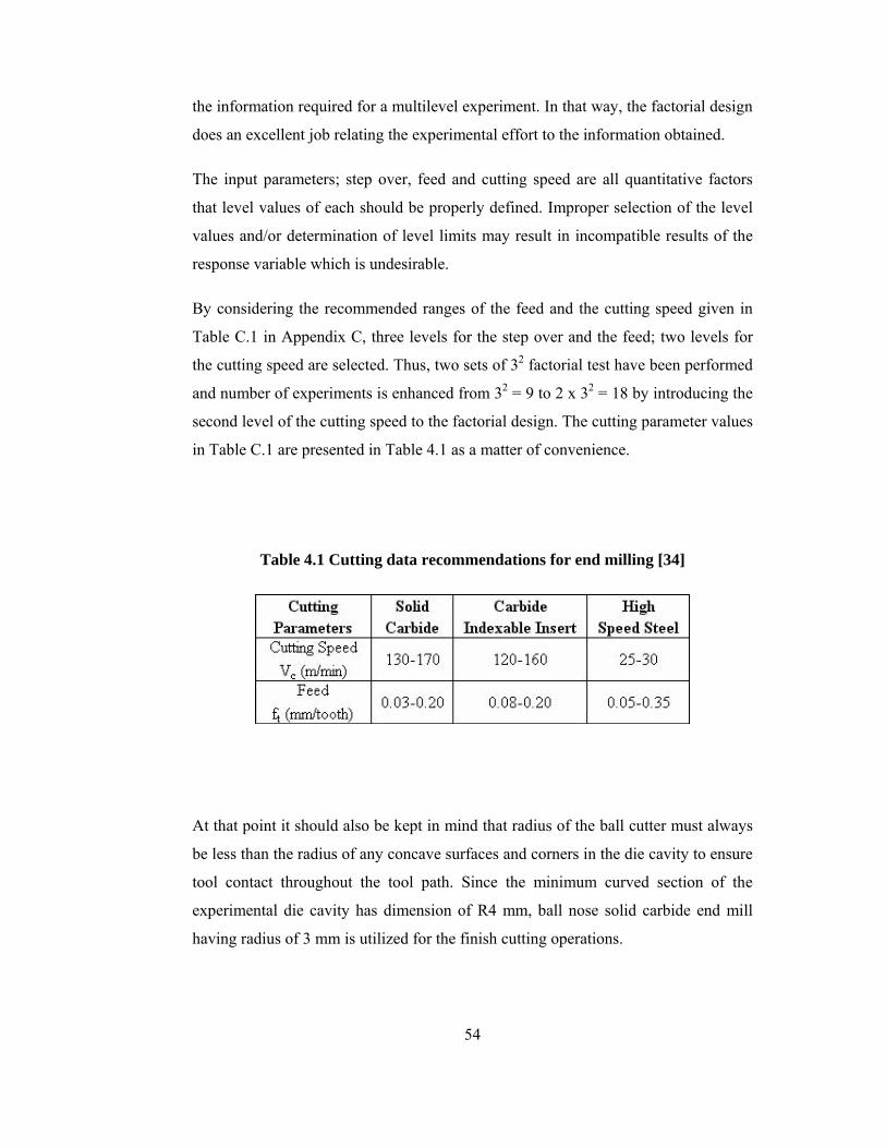
54
the information required for a multilevel experiment. In that way, the factorial design
does an excellent job relating the experimental effort to the information obtained.
The input parameters; step over, feed and cutting speed are all quantitative factors
that level values of each should be properly defined. Improper selection of the level
values and/or determination of level limits may result in incompatible results of the
response variable which is undesirable.
By considering the recommended ranges of the feed and the cutting speed given in
Table C.1 in Appendix C, three levels for the step over and the feed; two levels for
the cutting speed are selected. Thus, two sets of 32 factorial test have been performed
and number of experiments is enhanced from 32 = 9 to 2 x 32 = 18 by introducing the
second level of the cutting speed to the factorial design. The cutting parameter values
in Table C.1 are presented in Table 4.1 as a matter of convenience.
Table 4.1 Cutting data recommendations for end milling [34]
At that point it should also be kept in mind that radius of the ball cutter must always
be less than the radius of any concave surfaces and corners in the die cavity to ensure
tool contact throughout the tool path. Since the minimum curved section of the
experimental die cavity has dimension of R4 mm, ball nose solid carbide end mill
having radius of 3 mm is utilized for the finish cutting operations.
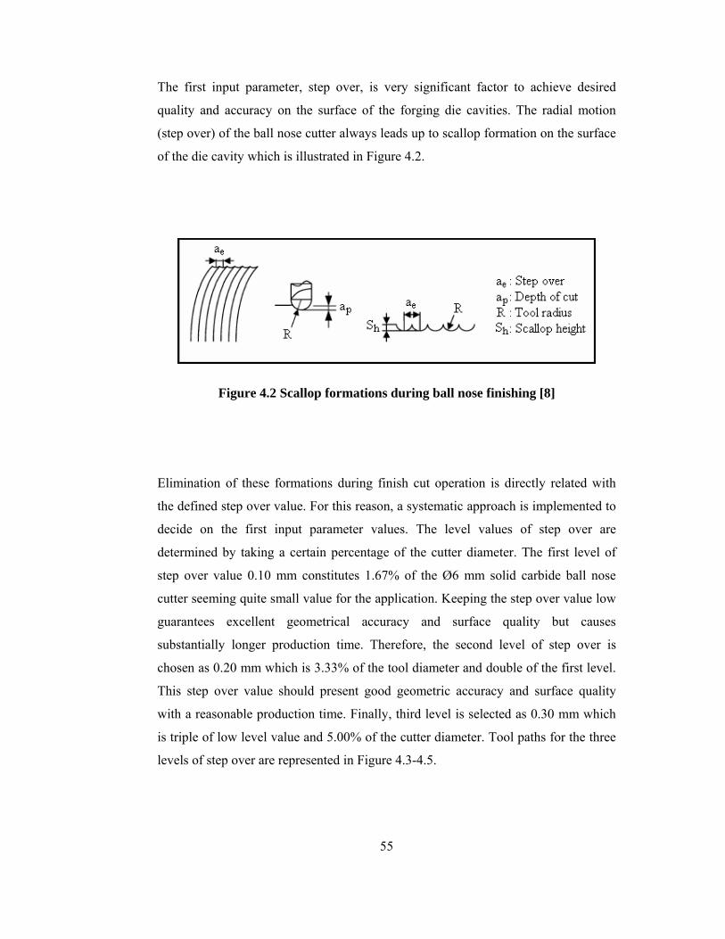
55
The first input parameter, step over, is very significant factor to achieve desired
quality and accuracy on the surface of the forging die cavities. The radial motion
(step over) of the ball nose cutter always leads up to scallop formation on the surface
of the die cavity which is illustrated in Figure 4.2.
Figure 4.2 Scallop formations during ball nose finishing [8]
Elimination of these formations during finish cut operation is directly related with
the defined step over value. For this reason, a systematic approach is implemented to
decide on the first input parameter values. The level values of step over are
determined by taking a certain percentage of the cutter diameter. The first level of
step over value 0.10 mm constitutes 1.67% of the Ø6 mm solid carbide ball nose
cutter seeming quite small value for the application. Keeping the step over value low
guarantees excellent geometrical accuracy and surface quality but causes
substantially longer production time. Therefore, the second level of step over is
chosen as 0.20 mm which is 3.33% of the tool diameter and double of the first level.
This step over value should present good geometric accuracy and surface quality
with a reasonable production time. Finally, third level is selected as 0.30 mm which
is triple of low level value and 5.00% of the cutter diameter. Tool paths for the three
levels of step over are represented in Figure 4.3-4.5.
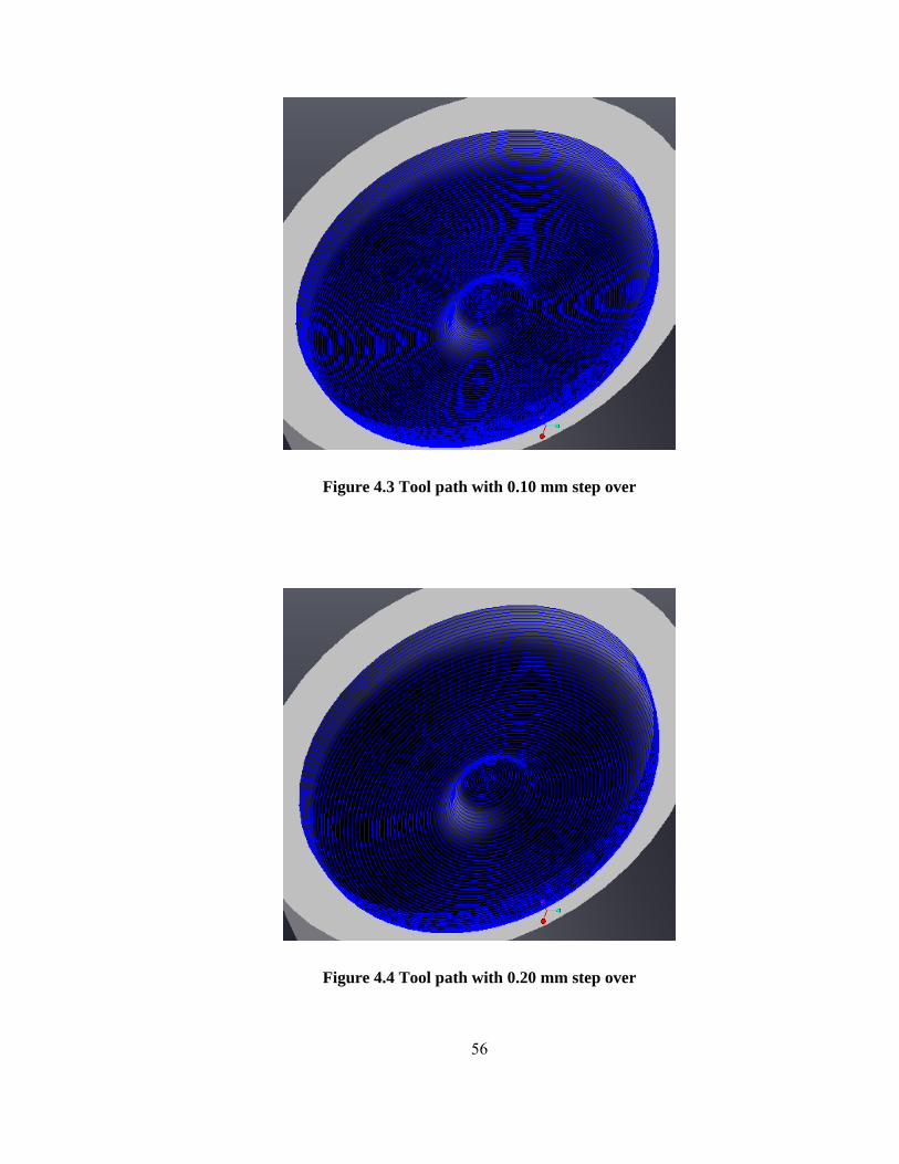
56
Figure 4.3 Tool path with 0.10 mm step over
Figure 4.4 Tool path with 0.20 mm step over
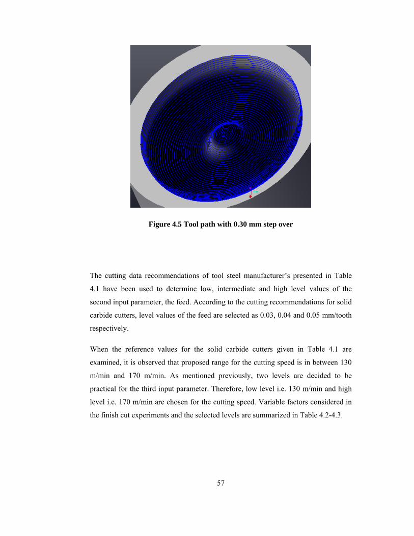
57
Figure 4.5 Tool path with 0.30 mm step over
The cutting data recommendations of tool steel manufacturer’s presented in Table
4.1 have been used to determine low, intermediate and high level values of the
second input parameter, the feed. According to the cutting recommendations for solid
carbide cutters, level values of the feed are selected as 0.03, 0.04 and 0.05 mm/tooth
respectively.
When the reference values for the solid carbide cutters given in Table 4.1 are
examined, it is observed that proposed range for the cutting speed is in between 130
m/min and 170 m/min. As mentioned previously, two levels are decided to be
practical for the third input parameter. Therefore, low level i.e. 130 m/min and high
level i.e. 170 m/min are chosen for the cutting speed. Variable factors considered in
the finish cut experiments and the selected levels are summarized in Table 4.2-4.3.
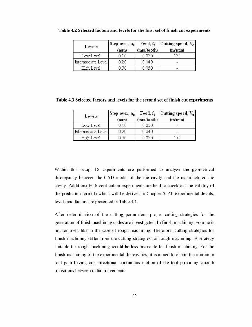
58
Table 4.2 Selected factors and levels for the first set of finish cut experiments
Table 4.3 Selected factors and levels for the second set of finish cut experiments
Within this setup, 18 experiments are performed to analyze the geometrical
discrepancy between the CAD model of the die cavity and the manufactured die
cavity. Additionally, 6 verification experiments are held to check out the validity of
the prediction formula which will be derived in Chapter 5. All experimental details,
levels and factors are presented in Table 4.4.
After determination of the cutting parameters, proper cutting strategies for the
generation of finish machining codes are investigated. In finish machining, volume is
not removed like in the case of rough machining. Therefore, cutting strategies for
finish machining differ from the cutting strategies for rough machining. A strategy
suitable for rough machining would be less favorable for finish machining. For the
finish machining of the experimental die cavities, it is aimed to obtain the minimum
tool path having one directional continuous motion of the tool providing smooth
transitions between radial movements.
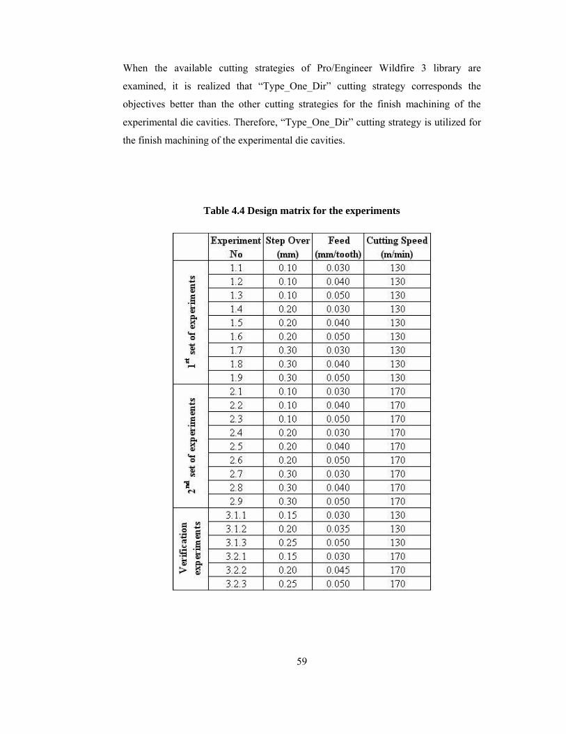
59
When the available cutting strategies of Pro/Engineer Wildfire 3 library are
examined, it is realized that “Type_One_Dir” cutting strategy corresponds the
objectives better than the other cutting strategies for the finish machining of the
experimental die cavities. Therefore, “Type_One_Dir” cutting strategy is utilized for
the finish machining of the experimental die cavities.
Table 4.4 Design matrix for the experiments
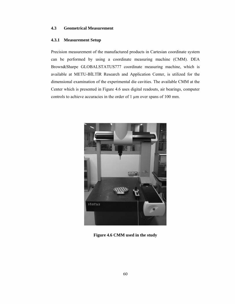
60
4.3 Geometrical Measurement
4.3.1 Measurement Setup
Precision measurement of the manufactured products in Cartesian coordinate system
can be performed by using a coordinate measuring machine (CMM). DEA
Brown&Sharpe GLOBALSTATUS777 coordinate measuring machine, which is
available at METU-BİLTİR Research and Application Center, is utilized for the
dimensional examination of the experimental die cavities. The available CMM at the
Center which is presented in Figure 4.6 uses digital readouts, air bearings, computer
controls to achieve accuracies in the order of 1 µm over spans of 100 mm.
Figure 4.6 CMM used in the study
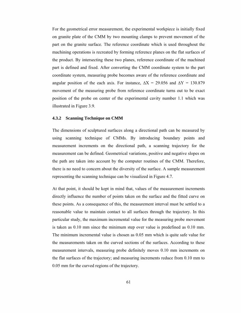
61
For the geometrical error measurement, the experimental workpiece is initially fixed
on granite plate of the CMM by two mounting clamps to prevent movement of the
part on the granite surface. The reference coordinate which is used throughout the
machining operations is recreated by forming reference planes on the flat surfaces of
the product. By intersecting these two planes, reference coordinate of the machined
part is defined and fixed. After converting the CMM coordinate system to the part
coordinate system, measuring probe becomes aware of the reference coordinate and
angular position of the each axis. For instance, ∆X = 29.056 and ∆Y = 130.879
movement of the measuring probe from reference coordinate turns out to be exact
position of the probe on center of the experimental cavity number 1.1 which was
illustrated in Figure 3.9.
4.3.2 Scanning Technique on CMM
The dimensions of sculptured surfaces along a directional path can be measured by
using scanning technique of CMMs. By introducing boundary points and
measurement increments on the directional path, a scanning trajectory for the
measurement can be defined. Geometrical variations, positive and negative slopes on
the path are taken into account by the computer routines of the CMM. Therefore,
there is no need to concern about the diversity of the surface. A sample measurement
representing the scanning technique can be visualized in Figure 4.7.
At that point, it should be kept in mind that, values of the measurement increments
directly influence the number of points taken on the surface and the fitted curve on
these points. As a consequence of this, the measurement interval must be settled to a
reasonable value to maintain contact to all surfaces through the trajectory. In this
particular study, the maximum incremental value for the measuring probe movement
is taken as 0.10 mm since the minimum step over value is predefined as 0.10 mm.
The minimum incremental value is chosen as 0.05 mm which is quite safe value for
the measurements taken on the curved sections of the surfaces. According to these
measurement intervals, measuring probe definitely moves 0.10 mm increments on
the flat surfaces of the trajectory; and measuring increments reduce from 0.10 mm to
0.05 mm for the curved regions of the trajectory.

62
Figure 4.7 Scanning technique on CMM
Since the experimental cavity geometry is axisymmetric, measurement along a
profile would be sufficient to represent the characteristics of the whole die cavity.
For the geometrical error analysis of the experimental die cavity, scanning is
performed in two directions which are orthogonal to each other. Scanning directions
of the experimental die cavity is represented in Figure 4.8.
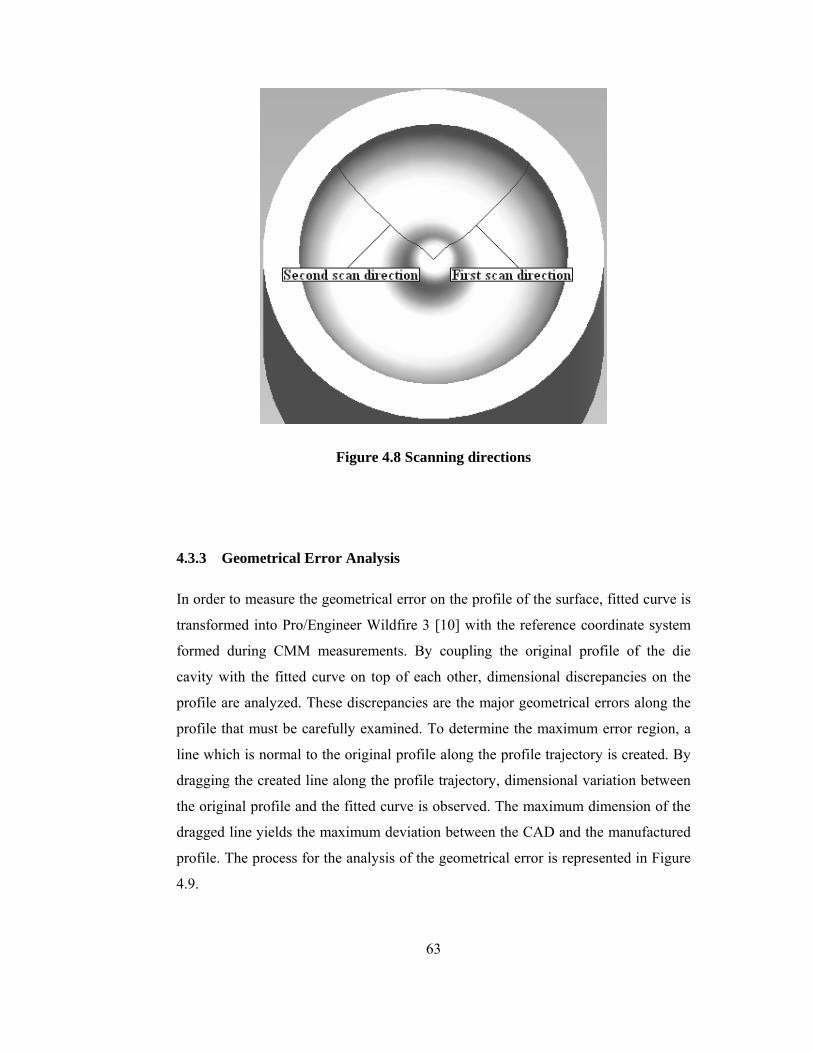
63
Figure 4.8 Scanning directions
4.3.3 Geometrical Error Analysis
In order to measure the geometrical error on the profile of the surface, fitted curve is
transformed into Pro/Engineer Wildfire 3 [10] with the reference coordinate system
formed during CMM measurements. By coupling the original profile of the die
cavity with the fitted curve on top of each other, dimensional discrepancies on the
profile are analyzed. These discrepancies are the major geometrical errors along the
profile that must be carefully examined. To determine the maximum error region, a
line which is normal to the original profile along the profile trajectory is created. By
dragging the created line along the profile trajectory, dimensional variation between
the original profile and the fitted curve is observed. The maximum dimension of the
dragged line yields the maximum deviation between the CAD and the manufactured
profile. The process for the analysis of the geometrical error is represented in Figure
4.9.
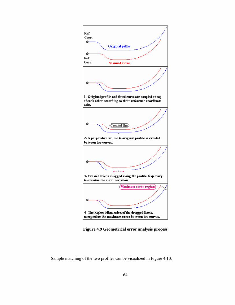
64
Figure 4.9 Geometrical error analysis process
Sample matching of the two profiles can be visualized in Figure 4.10.
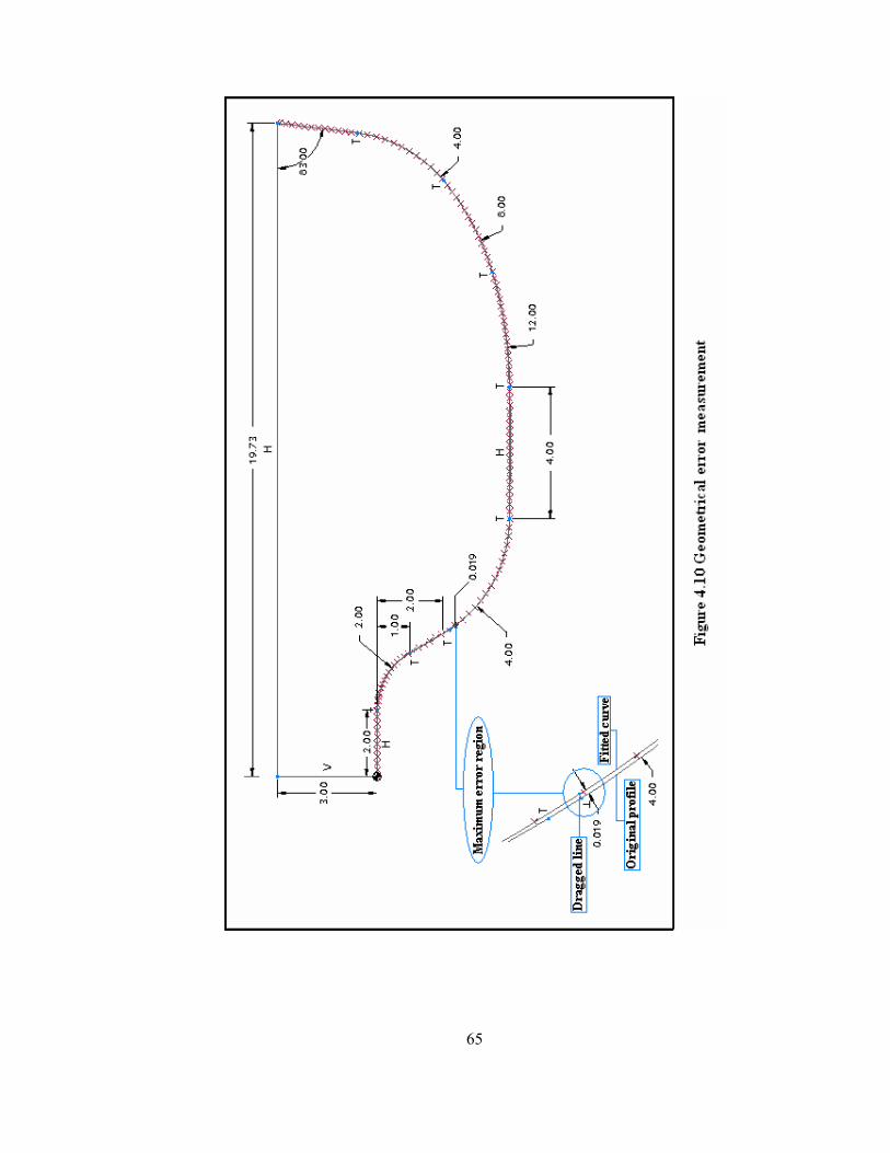
65

66
The measurement procedure is applied to the all die cavities manufactured in the
finish cut experiments. Analysis and results of the finish cut experiments will be
evaluated in Chapter 5.
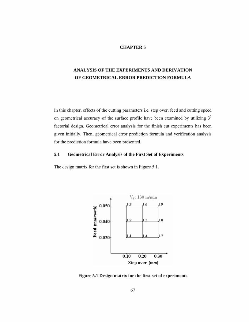
67
CHAPTER 5
ANALYSIS OF THE EXPERIMENTS AND DERIVATION
OF GEOMETRICAL ERROR PREDICTION FORMULA
In this chapter, effects of the cutting parameters i.e. step over, feed and cutting speed
on geometrical accuracy of the surface profile have been examined by utilizing 32
factorial design. Geometrical error analysis for the finish cut experiments has been
given initially. Then, geometrical error prediction formula and verification analysis
for the prediction formula have been presented.
5.1 Geometrical Error Analysis of the First Set of Experiments
The design matrix for the first set is shown in Figure 5.1.
Figure 5.1 Design matrix for the first set of experiments

68
With the application of the cutting parameter values described in Figure 5.1,
experimental die cavities involving surface and geometrical diversities are attained.
Manufactured die cavities in the first set of experiments are shown in Figure 5.2.
Figure 5.2 Photograph of the first set of experiments
The procedure for the geometrical error measurement between the CAD profile and
the manufactured profile was discussed in Section 4.3.3. According to this procedure,
the error measurements are performed and geometrical error variations of the first set
are obtained. Results of the geometrical error analysis for the first set of experiments
are presented in Table 5.1. The error measurements are performed in two scan
directions. Therefore, averages of the geometrical error measurements are also
tabulated in Table 5.1.
It can be observed from Table 5.1 that all geometrical error values are lower than 100
µm which is the predefined profile tolerance value for the experimental die cavity.
Therefore, all die cavities can be accepted as geometrically accurate in the defined
tolerance limits. However, when surface quality is taken into account, die cavities
having step over value of 0.10 mm are superior to the others. Depending on visual
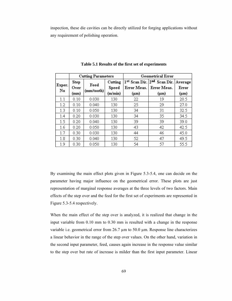
69
inspection, these die cavities can be directly utilized for forging applications without
any requirement of polishing operation.
Table 5.1 Results of the first set of experiments
By examining the main effect plots given in Figure 5.3-5.4, one can decide on the
parameter having major influence on the geometrical error. These plots are just
representation of marginal response averages at the three levels of two factors. Main
effects of the step over and the feed for the first set of experiments are represented in
Figure 5.3-5.4 respectively.
When the main effect of the step over is analyzed, it is realized that change in the
input variable from 0.10 mm to 0.30 mm is resulted with a change in the response
variable i.e. geometrical error from 26.7 µm to 50.0 µm. Response line characterizes
a linear behavior in the range of the step over values. On the other hand, variation in
the second input parameter, feed, causes again increase in the response value similar
to the step over but rate of increase is milder than the first input parameter. Linear
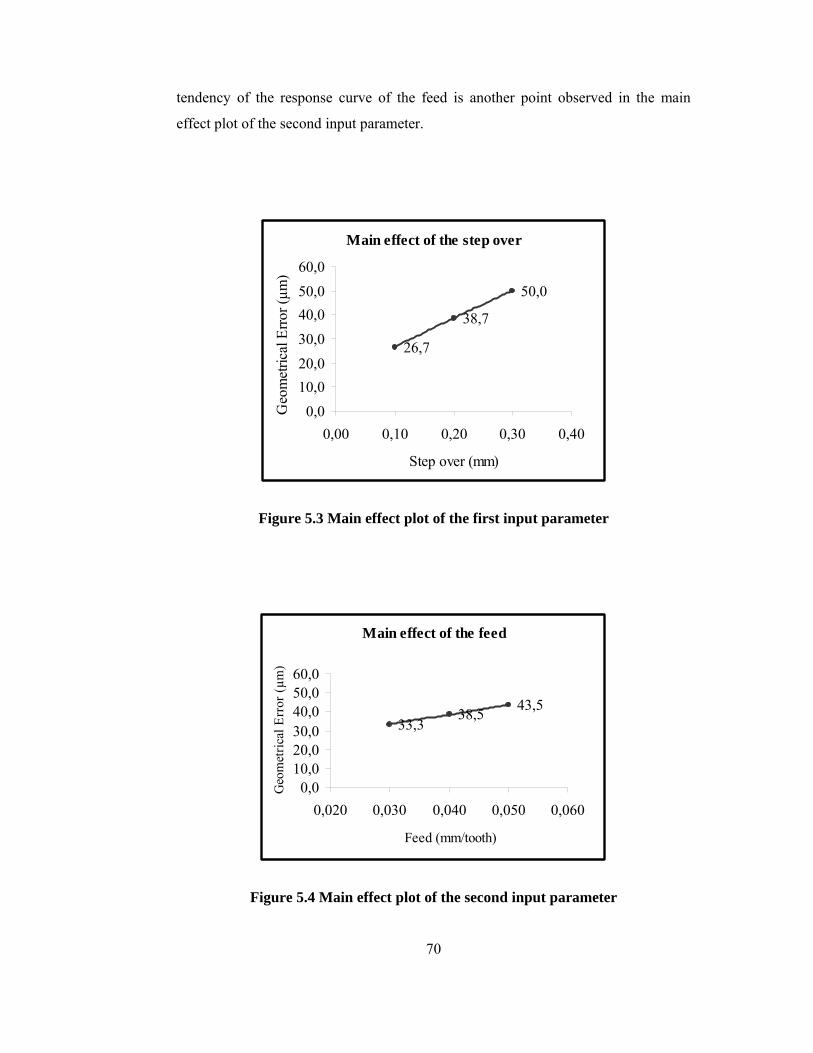
70
tendency of the response curve of the feed is another point observed in the main
effect plot of the second input parameter.
Main effect of the step over
26,7
38,7
50,0
0,010,020,030,040,050,060,0
0,00 0,10 0,20 0,30 0,40
Step over (mm)
Geo
met
rical
Erro
r (µm
)
Figure 5.3 Main effect plot of the first input parameter
Main effect of the feed
33,338,5 43,5
0,010,020,030,040,050,060,0
0,020 0,030 0,040 0,050 0,060
Feed (mm/tooth)
Geo
met
rical
Err
or (µ
m)
Figure 5.4 Main effect plot of the second input parameter
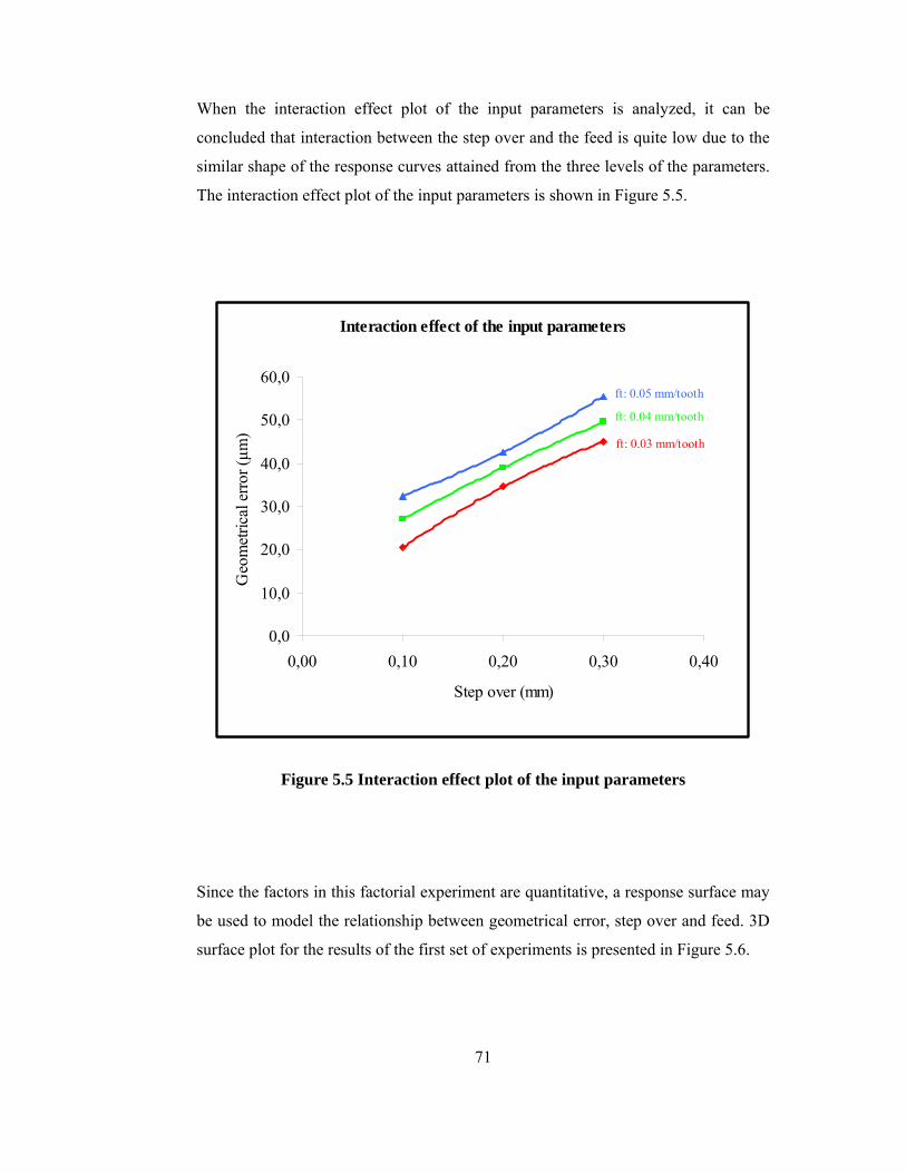
71
When the interaction effect plot of the input parameters is analyzed, it can be
concluded that interaction between the step over and the feed is quite low due to the
similar shape of the response curves attained from the three levels of the parameters.
The interaction effect plot of the input parameters is shown in Figure 5.5.
Interaction effect of the input parameters
ft: 0.03 mm/tooth
ft: 0.04 mm/tooth
ft: 0.05 mm/tooth
0,0
10,0
20,0
30,0
40,0
50,0
60,0
0,00 0,10 0,20 0,30 0,40
Step over (mm)
Geo
met
rical
erro
r (µm
)
Figure 5.5 Interaction effect plot of the input parameters
Since the factors in this factorial experiment are quantitative, a response surface may
be used to model the relationship between geometrical error, step over and feed. 3D
surface plot for the results of the first set of experiments is presented in Figure 5.6.
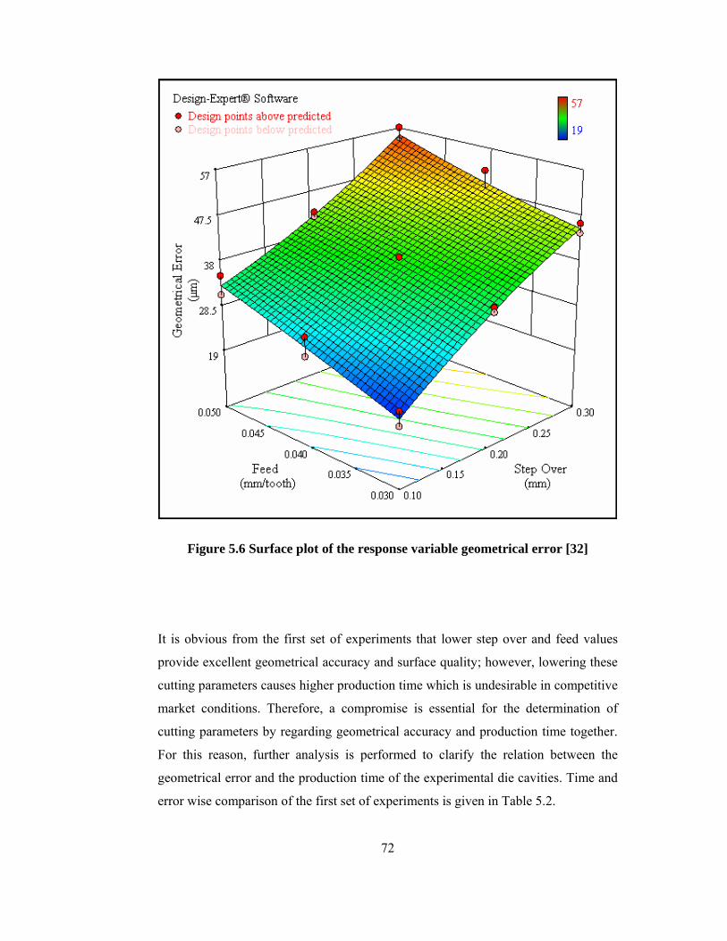
72
Figure 5.6 Surface plot of the response variable geometrical error [32]
It is obvious from the first set of experiments that lower step over and feed values
provide excellent geometrical accuracy and surface quality; however, lowering these
cutting parameters causes higher production time which is undesirable in competitive
market conditions. Therefore, a compromise is essential for the determination of
cutting parameters by regarding geometrical accuracy and production time together.
For this reason, further analysis is performed to clarify the relation between the
geometrical error and the production time of the experimental die cavities. Time and
error wise comparison of the first set of experiments is given in Table 5.2.
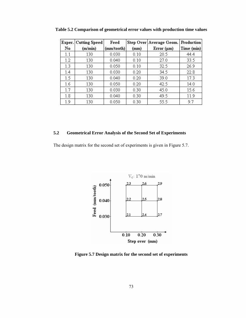
73
Table 5.2 Comparison of geometrical error values with production time values
5.2 Geometrical Error Analysis of the Second Set of Experiments
The design matrix for the second set of experiments is given in Figure 5.7.
Figure 5.7 Design matrix for the second set of experiments
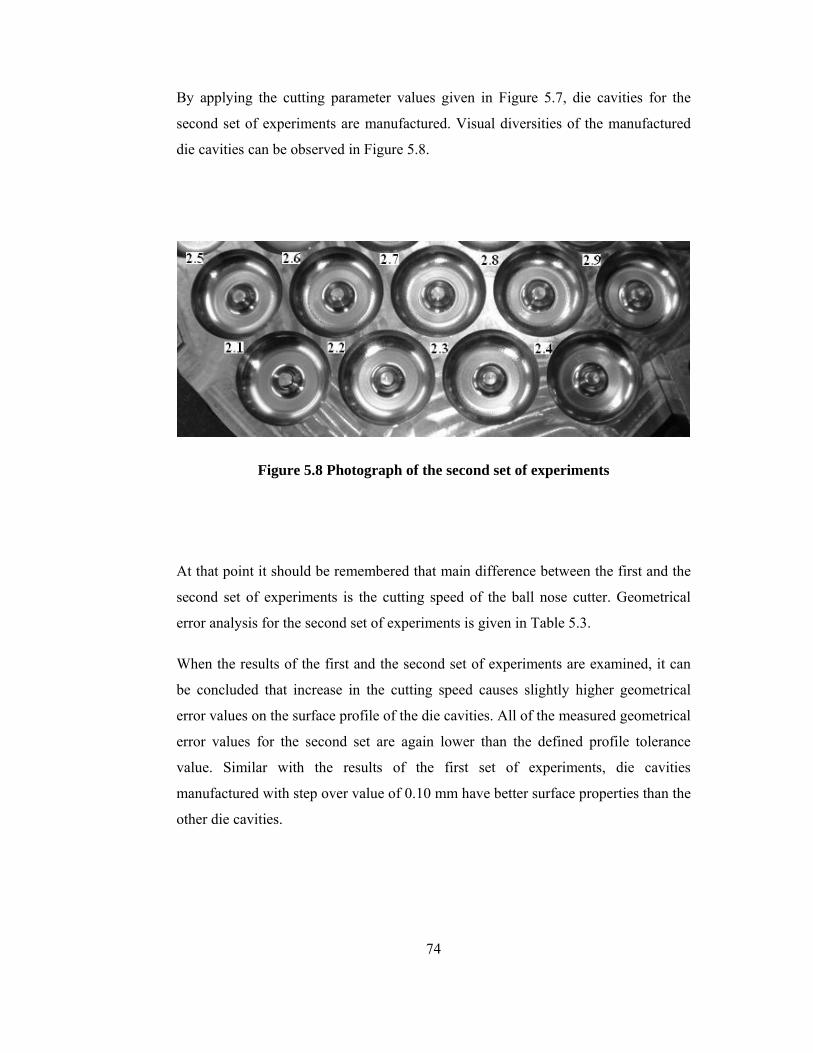
74
By applying the cutting parameter values given in Figure 5.7, die cavities for the
second set of experiments are manufactured. Visual diversities of the manufactured
die cavities can be observed in Figure 5.8.
Figure 5.8 Photograph of the second set of experiments
At that point it should be remembered that main difference between the first and the
second set of experiments is the cutting speed of the ball nose cutter. Geometrical
error analysis for the second set of experiments is given in Table 5.3.
When the results of the first and the second set of experiments are examined, it can
be concluded that increase in the cutting speed causes slightly higher geometrical
error values on the surface profile of the die cavities. All of the measured geometrical
error values for the second set are again lower than the defined profile tolerance
value. Similar with the results of the first set of experiments, die cavities
manufactured with step over value of 0.10 mm have better surface properties than the
other die cavities.
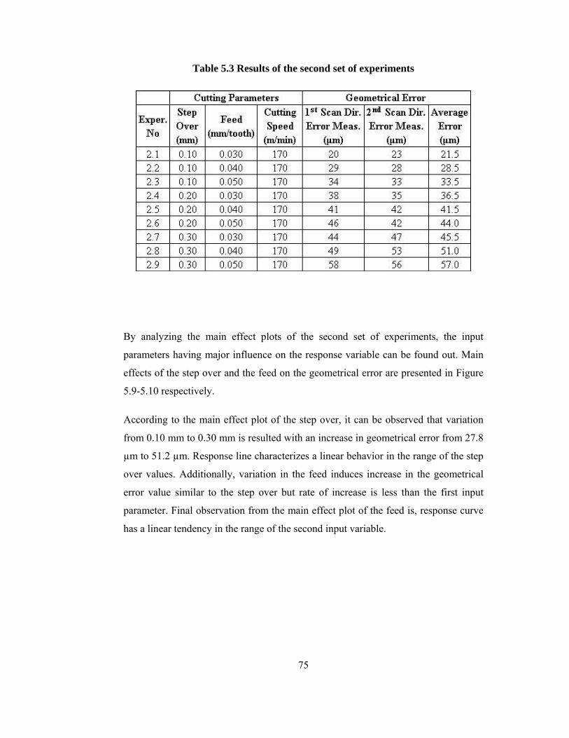
75
Table 5.3 Results of the second set of experiments
By analyzing the main effect plots of the second set of experiments, the input
parameters having major influence on the response variable can be found out. Main
effects of the step over and the feed on the geometrical error are presented in Figure
5.9-5.10 respectively.
According to the main effect plot of the step over, it can be observed that variation
from 0.10 mm to 0.30 mm is resulted with an increase in geometrical error from 27.8
µm to 51.2 µm. Response line characterizes a linear behavior in the range of the step
over values. Additionally, variation in the feed induces increase in the geometrical
error value similar to the step over but rate of increase is less than the first input
parameter. Final observation from the main effect plot of the feed is, response curve
has a linear tendency in the range of the second input variable.
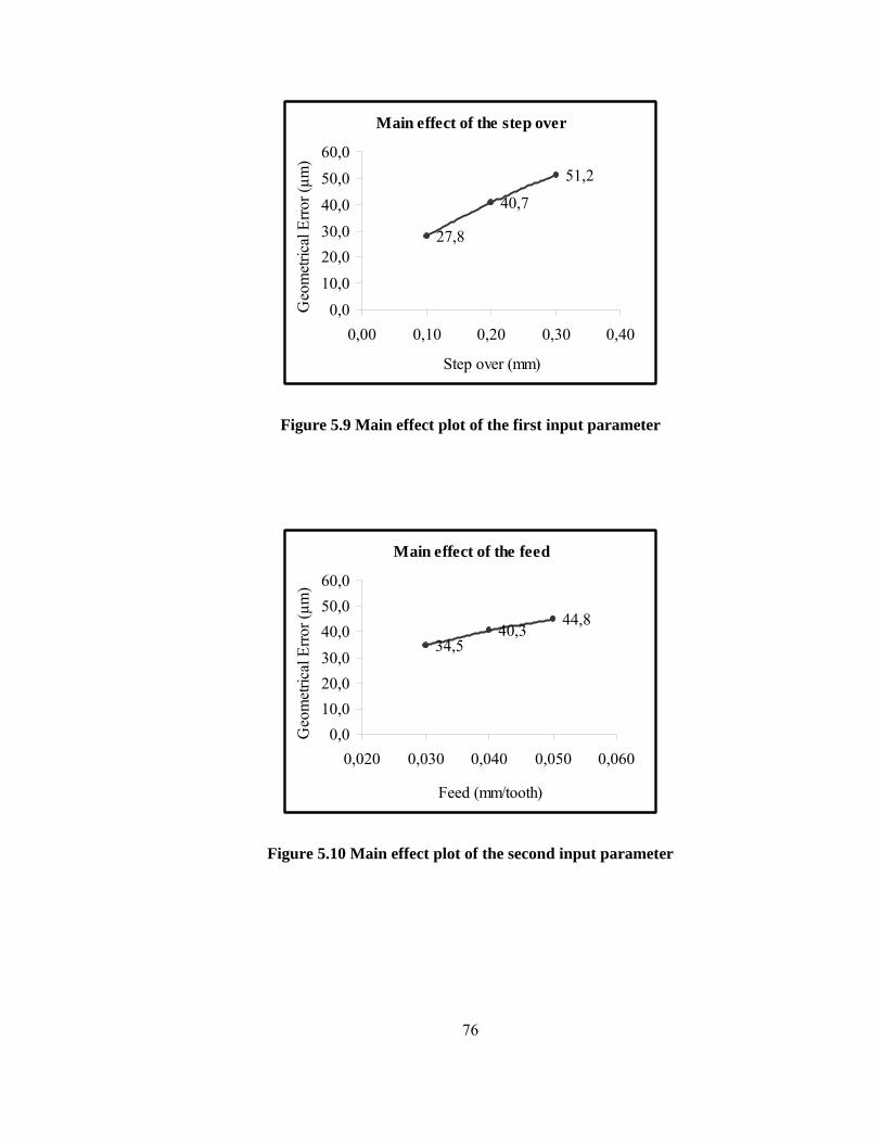
76
Main effect of the step over
27,8
40,7
51,2
0,010,020,030,040,050,060,0
0,00 0,10 0,20 0,30 0,40
Step over (mm)
Geo
met
rical
Erro
r (µm
)
Figure 5.9 Main effect plot of the first input parameter
Main effect of the feed
34,540,3
44,8
0,010,020,030,040,050,060,0
0,020 0,030 0,040 0,050 0,060
Feed (mm/tooth)
Geo
met
rical
Erro
r (µm
)
Figure 5.10 Main effect plot of the second input parameter
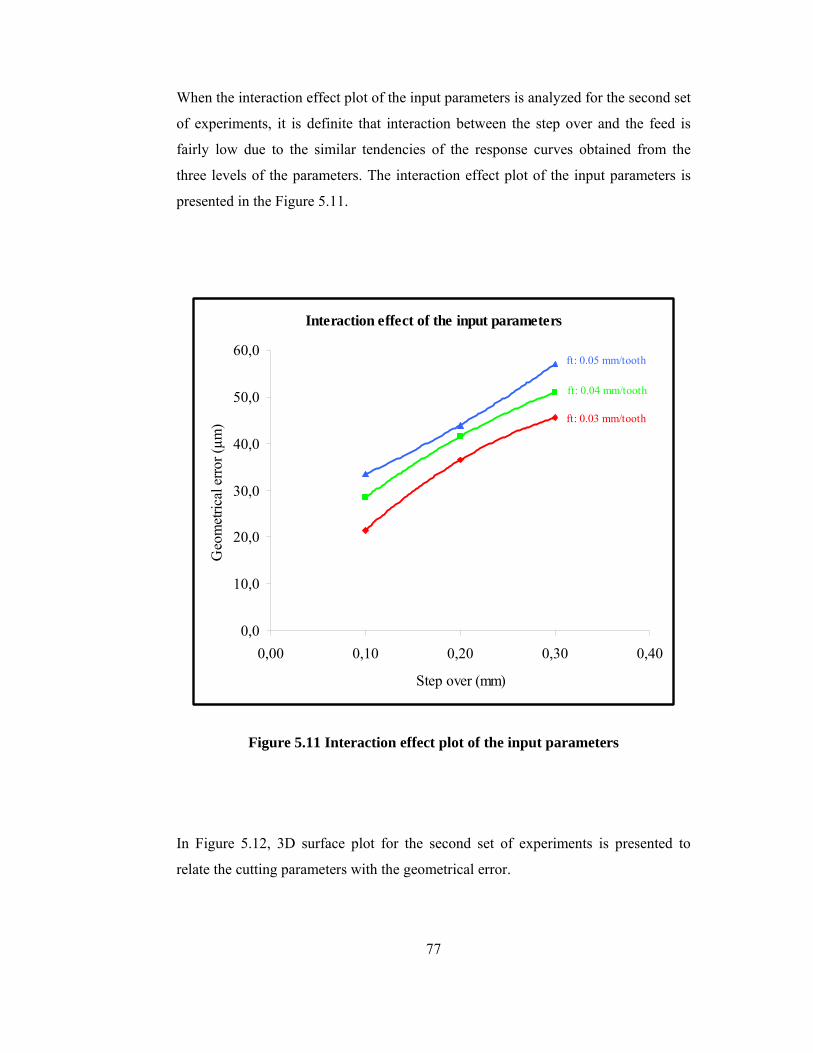
77
When the interaction effect plot of the input parameters is analyzed for the second set
of experiments, it is definite that interaction between the step over and the feed is
fairly low due to the similar tendencies of the response curves obtained from the
three levels of the parameters. The interaction effect plot of the input parameters is
presented in the Figure 5.11.
Interaction effect of the input parameters
ft: 0.03 mm/tooth
ft: 0.04 mm/tooth
ft: 0.05 mm/tooth
0,0
10,0
20,0
30,0
40,0
50,0
60,0
0,00 0,10 0,20 0,30 0,40
Step over (mm)
Geo
met
rical
erro
r (µm
)
Figure 5.11 Interaction effect plot of the input parameters
In Figure 5.12, 3D surface plot for the second set of experiments is presented to
relate the cutting parameters with the geometrical error.
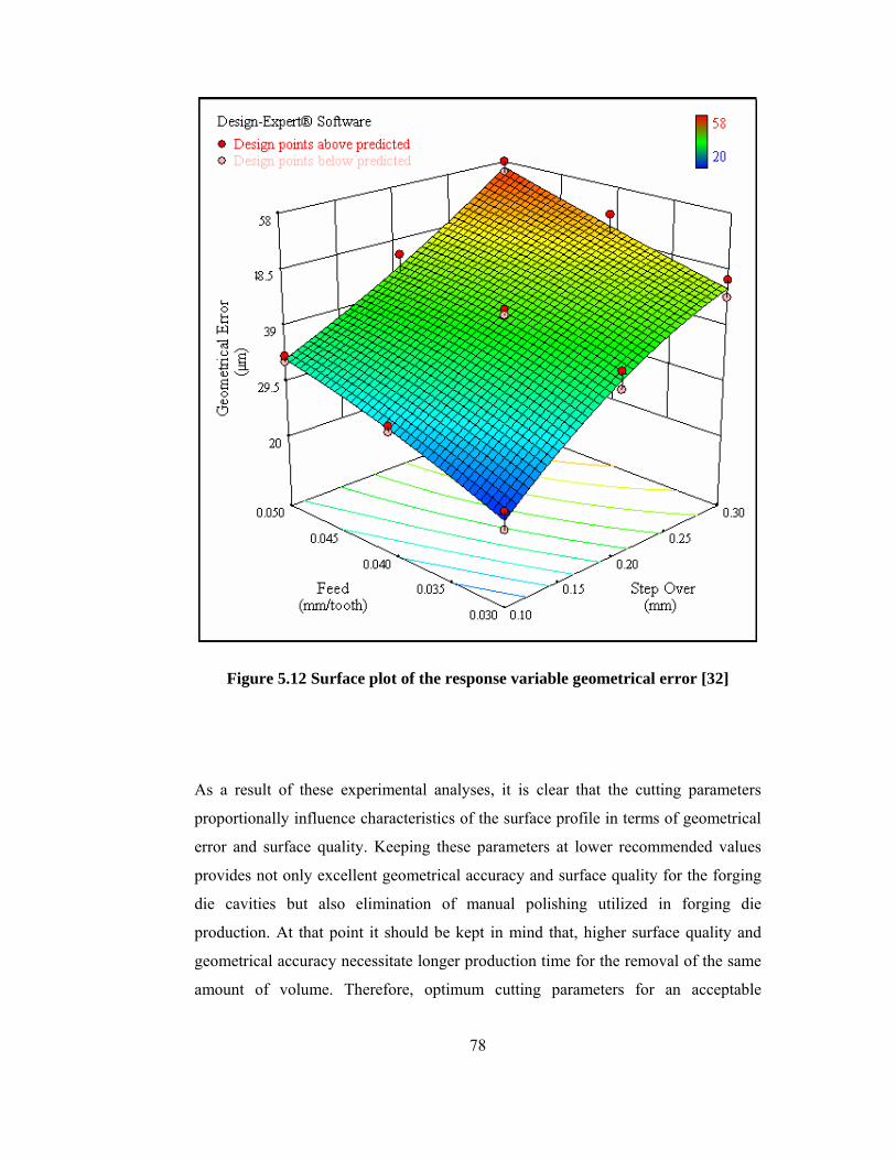
78
Figure 5.12 Surface plot of the response variable geometrical error [32]
As a result of these experimental analyses, it is clear that the cutting parameters
proportionally influence characteristics of the surface profile in terms of geometrical
error and surface quality. Keeping these parameters at lower recommended values
provides not only excellent geometrical accuracy and surface quality for the forging
die cavities but also elimination of manual polishing utilized in forging die
production. At that point it should be kept in mind that, higher surface quality and
geometrical accuracy necessitate longer production time for the removal of the same
amount of volume. Therefore, optimum cutting parameters for an acceptable
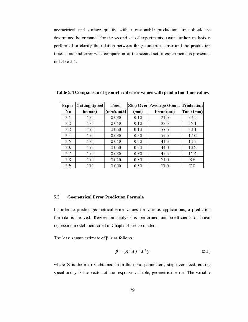
79
geometrical and surface quality with a reasonable production time should be
determined beforehand. For the second set of experiments, again further analysis is
performed to clarify the relation between the geometrical error and the production
time. Time and error wise comparison of the second set of experiments is presented
in Table 5.4.
Table 5.4 Comparison of geometrical error values with production time values
5.3 Geometrical Error Prediction Formula
In order to predict geometrical error values for various applications, a prediction
formula is derived. Regression analysis is performed and coefficients of linear
regression model mentioned in Chapter 4 are computed.
The least square estimate of β is as follows:
yXXX TT 1)( −=β (5.1)
where X is the matrix obtained from the input parameters, step over, feed, cutting
speed and y is the vector of the response variable, geometrical error. The variable
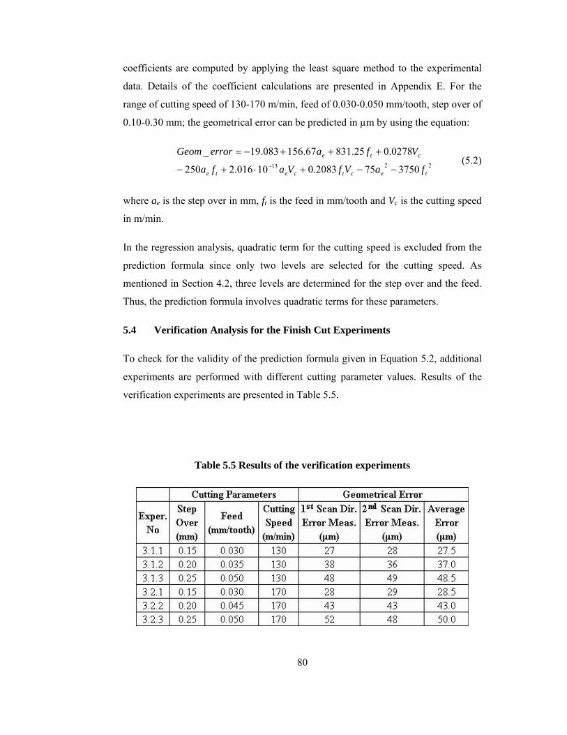
80
coefficients are computed by applying the least square method to the experimental
data. Details of the coefficient calculations are presented in Appendix E. For the
range of cutting speed of 130-170 m/min, feed of 0.030-0.050 mm/tooth, step over of
0.10-0.30 mm; the geometrical error can be predicted in µm by using the equation:
2213 3750752083.010016.2250
0278.025.83167.156083.19_
tectcete
cte
faVfVafa
VfaerrorGeom
−−+⋅+−
+++−=−
(5.2)
where ae is the step over in mm, ft is the feed in mm/tooth and Vc is the cutting speed
in m/min.
In the regression analysis, quadratic term for the cutting speed is excluded from the
prediction formula since only two levels are selected for the cutting speed. As
mentioned in Section 4.2, three levels are determined for the step over and the feed.
Thus, the prediction formula involves quadratic terms for these parameters.
5.4 Verification Analysis for the Finish Cut Experiments
To check for the validity of the prediction formula given in Equation 5.2, additional
experiments are performed with different cutting parameter values. Results of the
verification experiments are presented in Table 5.5.
Table 5.5 Results of the verification experiments
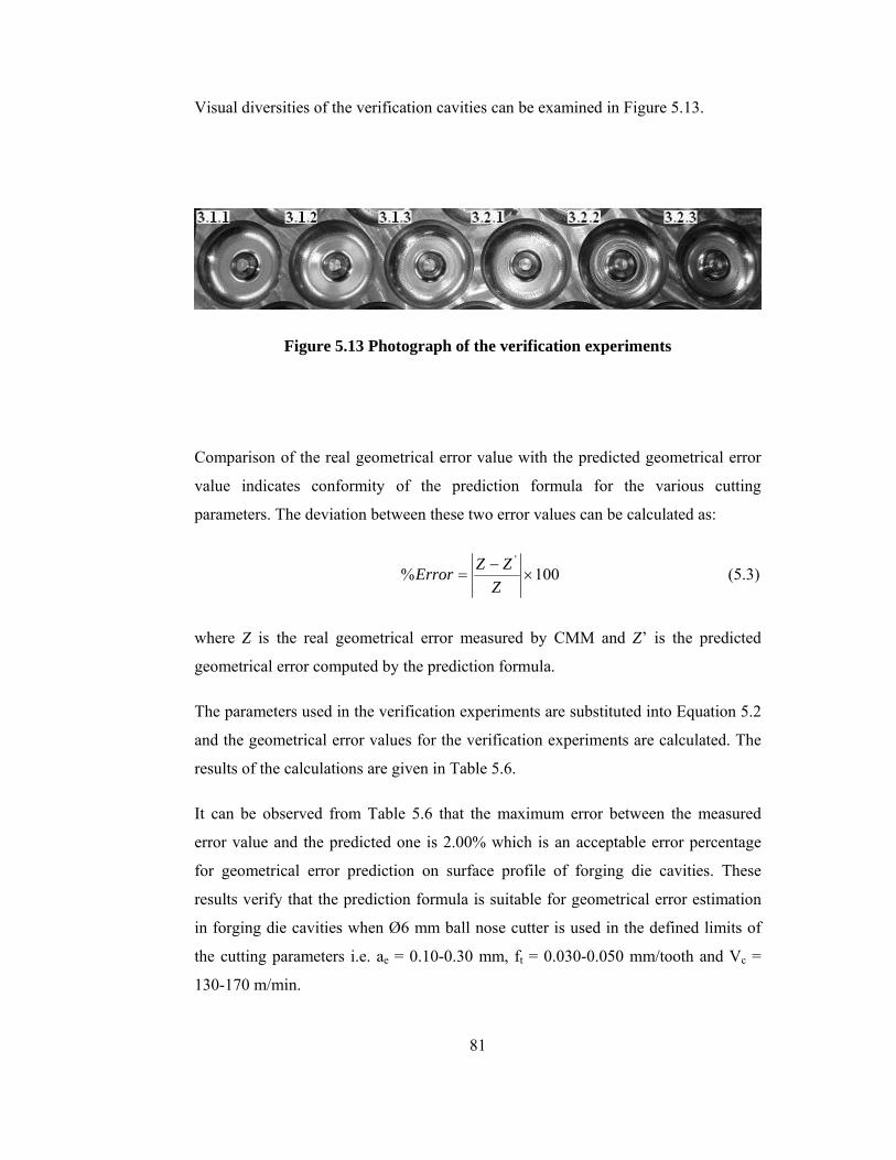
81
Visual diversities of the verification cavities can be examined in Figure 5.13.
Figure 5.13 Photograph of the verification experiments
Comparison of the real geometrical error value with the predicted geometrical error
value indicates conformity of the prediction formula for the various cutting
parameters. The deviation between these two error values can be calculated as:
100%'
×−
=Z
ZZError (5.3)
where Z is the real geometrical error measured by CMM and Z’ is the predicted
geometrical error computed by the prediction formula.
The parameters used in the verification experiments are substituted into Equation 5.2
and the geometrical error values for the verification experiments are calculated. The
results of the calculations are given in Table 5.6.
It can be observed from Table 5.6 that the maximum error between the measured
error value and the predicted one is 2.00% which is an acceptable error percentage
for geometrical error prediction on surface profile of forging die cavities. These
results verify that the prediction formula is suitable for geometrical error estimation
in forging die cavities when Ø6 mm ball nose cutter is used in the defined limits of
the cutting parameters i.e. ae = 0.10-0.30 mm, ft = 0.030-0.050 mm/tooth and Vc =
130-170 m/min.
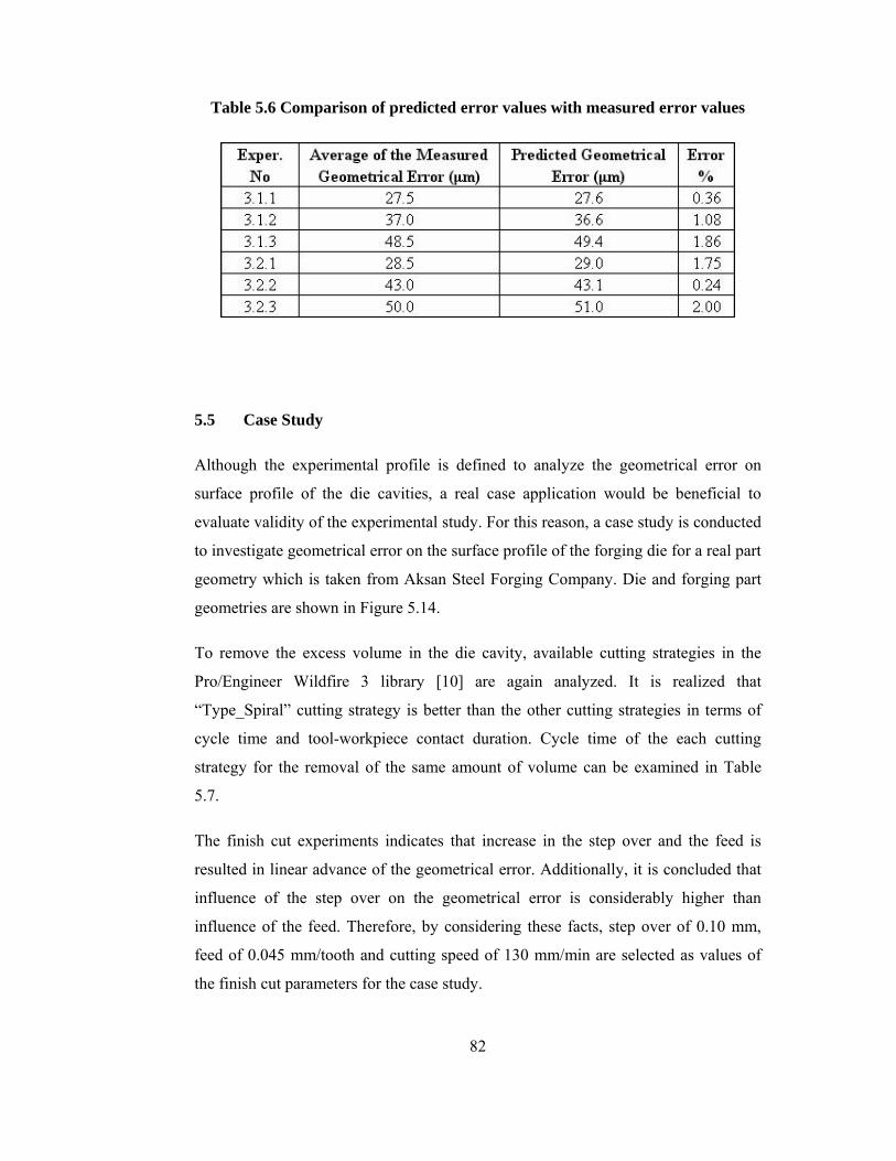
82
Table 5.6 Comparison of predicted error values with measured error values
5.5 Case Study
Although the experimental profile is defined to analyze the geometrical error on
surface profile of the die cavities, a real case application would be beneficial to
evaluate validity of the experimental study. For this reason, a case study is conducted
to investigate geometrical error on the surface profile of the forging die for a real part
geometry which is taken from Aksan Steel Forging Company. Die and forging part
geometries are shown in Figure 5.14.
To remove the excess volume in the die cavity, available cutting strategies in the
Pro/Engineer Wildfire 3 library [10] are again analyzed. It is realized that
“Type_Spiral” cutting strategy is better than the other cutting strategies in terms of
cycle time and tool-workpiece contact duration. Cycle time of the each cutting
strategy for the removal of the same amount of volume can be examined in Table
5.7.
The finish cut experiments indicates that increase in the step over and the feed is
resulted in linear advance of the geometrical error. Additionally, it is concluded that
influence of the step over on the geometrical error is considerably higher than
influence of the feed. Therefore, by considering these facts, step over of 0.10 mm,
feed of 0.045 mm/tooth and cutting speed of 130 mm/min are selected as values of
the finish cut parameters for the case study.
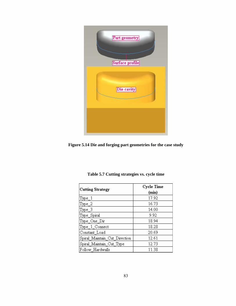
83
Figure 5.14 Die and forging part geometries for the case study
Table 5.7 Cutting strategies vs. cycle time
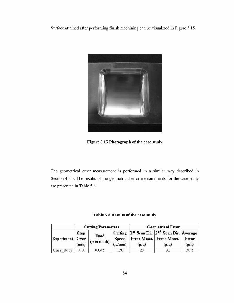
84
Surface attained after performing finish machining can be visualized in Figure 5.15.
Figure 5.15 Photograph of the case study
The geometrical error measurement is performed in a similar way described in
Section 4.3.3. The results of the geometrical error measurements for the case study
are presented in Table 5.8.
Table 5.8 Results of the case study
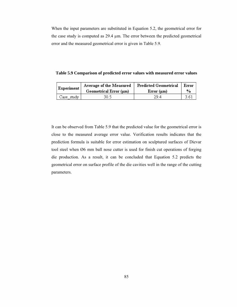
85
When the input parameters are substituted in Equation 5.2, the geometrical error for
the case study is computed as 29.4 µm. The error between the predicted geometrical
error and the measured geometrical error is given in Table 5.9.
Table 5.9 Comparison of predicted error values with measured error values
It can be observed from Table 5.9 that the predicted value for the geometrical error is
close to the measured average error value. Verification results indicates that the
prediction formula is suitable for error estimation on sculptured surfaces of Dievar
tool steel when Ø6 mm ball nose cutter is used for finish cut operations of forging
die production. As a result, it can be concluded that Equation 5.2 predicts the
geometrical error on surface profile of the die cavities well in the range of the cutting
parameters.
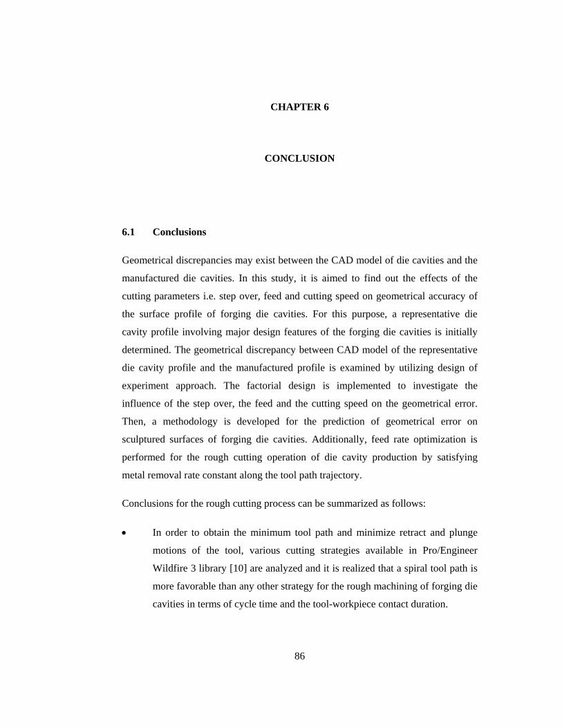
86
CHAPTER 6
CONCLUSION
6.1 Conclusions
Geometrical discrepancies may exist between the CAD model of die cavities and the
manufactured die cavities. In this study, it is aimed to find out the effects of the
cutting parameters i.e. step over, feed and cutting speed on geometrical accuracy of
the surface profile of forging die cavities. For this purpose, a representative die
cavity profile involving major design features of the forging die cavities is initially
determined. The geometrical discrepancy between CAD model of the representative
die cavity profile and the manufactured profile is examined by utilizing design of
experiment approach. The factorial design is implemented to investigate the
influence of the step over, the feed and the cutting speed on the geometrical error.
Then, a methodology is developed for the prediction of geometrical error on
sculptured surfaces of forging die cavities. Additionally, feed rate optimization is
performed for the rough cutting operation of die cavity production by satisfying
metal removal rate constant along the tool path trajectory.
Conclusions for the rough cutting process can be summarized as follows:
• In order to obtain the minimum tool path and minimize retract and plunge
motions of the tool, various cutting strategies available in Pro/Engineer
Wildfire 3 library [10] are analyzed and it is realized that a spiral tool path is
more favorable than any other strategy for the rough machining of forging die
cavities in terms of cycle time and the tool-workpiece contact duration.
87
• Lower metal removal rate in some sections of the tool path due to lower step
over value than the specified step over value, is common deficiency of the
cutting strategies available in the CAM module of Pro/Engineer Wildfire 3
[10]. This problem exists also for the application of the spiral tool path. The
spiral tool path for the experimental die cavity geometry is refined by the feed
rate optimization to provide the constant metal removal rate along the tool
path trajectory. Instead of using a single feed rate value which is 594
mm/min, different and higher feed rate values are utilized along the tool path
trajectory. Depending on the geometrical considerations, feed rate values are
increased up to 1500 mm/min for cutting process. For the motions of the tool
in air, feed rate value of 2000 mm/min is applied. As a consequence of the
performed optimization, the metal removal rate is kept at 475.2 mm3/min by
introducing higher feed rate values in the surface regions of the die cavity
where step over value is less than 4 mm. As expected, increase in the feed
rate values results in a reduction in the production time of the rough cutting
operation. It takes 18.75 min. when the original tool path is used to remove
the same amount of volume but with the implementation of higher feed rate
values to the machining code, the time required has been reduced to 14.22
min. As a result of this optimization, approximately 24.2% time reduction is
attained for the rough machining of the experimental die cavity geometry.
The following conclusions have been reached as results of the finish cut experiments:
• In the first set of experiments where the cutting speed is 130 m/min, it is
observed that the variation in the step over is more influential than the
variation in the feed to the geometrical error. When the main effect plot of the
step over is examined, it is realized that the geometrical error averages are
26.7 µm, 38.7 µm and 50.0 µm. The geometrical error averages due to the
feed variation are close to each other and observed as 33.3 µm, 38.5 µm and
43.5 µm indicating that feed variation is less effective on the geometrical
error than the step over variation.
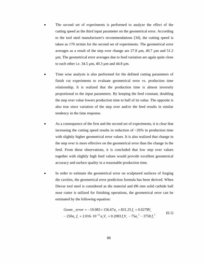
88
• The second set of experiments is performed to analyze the effect of the
cutting speed as the third input parameter on the geometrical error. According
to the tool steel manufacturer's recommendations [34], the cutting speed is
taken as 170 m/min for the second set of experiments. The geometrical error
averages as a result of the step over change are 27.8 µm, 40.7 µm and 51.2
µm. The geometrical error averages due to feed variation are again quite close
to each other i.e. 34.5 µm, 40.3 µm and 44.8 µm.
• Time wise analysis is also performed for the defined cutting parameters of
finish cut experiments to evaluate geometrical error vs. production time
relationship. It is realized that the production time is almost inversely
proportional to the input parameters. By keeping the feed constant, doubling
the step over value lowers production time to half of its value. The opposite is
also true since variation of the step over and/or the feed results in similar
tendency in the time response.
• As a consequence of the first and the second set of experiments, it is clear that
increasing the cutting speed results in reduction of ~26% in production time
with slightly higher geometrical error values. It is also realized that change in
the step over is more effective on the geometrical error than the change in the
feed. From these observations, it is concluded that low step over values
together with slightly high feed values would provide excellent geometrical
accuracy and surface quality in a reasonable production time.
• In order to estimate the geometrical error on sculptured surfaces of forging
die cavities, the geometrical error prediction formula has been derived. When
Dievar tool steel is considered as die material and Ø6 mm solid carbide ball
nose cutter is utilized for finishing operations, the geometrical error can be
estimated by the following equation:
2213 3750752083.010016.2250
0278.025.83167.156083.19_
tectcete
cte
faVfVafa
VfaerrorGeom
−−+⋅+−
+++−=−
(6.1)
89
where ae is the step over in mm, ft is the feed in mm/tooth and Vc is the
cutting speed in m/min.
• Validity of the prediction formula is tested by performing verification
experiments for the representative die geometry and a die cavity geometry of
a forging part used in industry. The maximum prediction error is observed as
3.61% indicating that the prediction formula is good enough for the error
estimation on sculptured surfaces of Dievar tool steel. Therefore, it is
concluded that the derived mathematical model is promising to be applicable
for geometrical error prediction on the surface profile of the forging die
cavities in the chosen range of the cutting parameters i.e. ae = 0.10-0.30 mm,
ft = 0.030-0.050 mm/tooth and Vc = 130-170 m/min.
6.2 Recommendations for Future Work
• The cutting strategies of other CAM software systems may be analyzed and
compared with Pro/Engineer Wildfire 3 library. In case of superior strategy
than the spiral tool path, this strategy may be exposed to optimization for the
rough machining process of forging dies.
• This work may be extended for different type and size of milling cutters.
• Cutting parameter values higher than the recommended values may be
utilized for the finish cut experiments to investigate the geometrical error
variation in the outside of the proposed range of the parameters.
• Similar study may be conducted to analyze the effects of cutting parameters
on surface roughness of the die cavities.
• The effects of cutting parameters on tool life may be studied and the ways to
improve the tool life may be investigated.
• Cutting forces may be calculated for various positions of the cutter during
machining of sculptured surfaces.
90
REFERENCES
[1] Boyer H., “Metals Handbook Forging and Casting”, (1971) ASM Handbook Committee, 8th Edition.
[2] Strecon, web site: “http://www.strecon.com”, last accessed: September 2007.
[3] Forging Industry Association, web site: “http://www.forging.org/facts”, last accessed: August 2007.
[4] Aksan Steel Forging Company, web site: “http://www.aksanforging.com”, last accessed: October 2007.
[5] Ghanem F., Braham C., Sidhom H., “Influence of steel type on electrical discharge machined surface integrity”, Journal of Materials Processing Technology, 142 (2003) 163-173.
[6] Cusanelli G., Hessler Wyser A., Bobard F., Demellayer R., Perez R., Flükiger R., “Microstructure at submicron scale of the white layer produced by EDM technique”, Journal of Materials Processing Technology, 149 (2004) 289-295.
[7] P. FallboEhmer, C.A. RodroAguez, T. Ozel, T. Altan, “High speed machining of cast iron and alloy steels for die and mold manufacturing”, Journal of Materials Processing Technology, 98 (2000) 104-115.
[8] B. Kecelj, J. Kopac, Z. Kampus, K. Kuzman, “Speciality of HSC in manufacturing of forging dies”, Journal of Materials Processing Technology 157-158 (2004) 536-542.

91
[9] J. Vivancos, C.J. Lui, L. Costa, J.A. Ortiz, “Optimal machining parameters selection in high speed milling of hardened steels for injection moulds”, Journal of Materials Processing Technology, 155-156 (2004) 1505-1512.
[10] Manufacturing Module of Pro/Engineer Wildfire 3.
[11] L.N. Lopez de Lacalle, A. Lamikiz, J.A. Sanchez, J.L. Arana, “Improving the surface finish in high speed milling of stamping dies”, Journal of Materials Processing Technology 123 (2002) 292-302.
[12] R.T. Coelho, L.R. Silva, A. Braghini, A.A. Bezerra, “Some effects of cutting edge preparation and geometric modifications when turning INCONEL 718TM at high cutting speeds”, Journal of Materials Processing Technology 148 (2004) 147-153.
[13] A. Kaldos, I.F. Dagiloke, A. Boyle, “Computer aided cutting process parameter selection for high speed milling”, Journal of Materials Processing Technology 61 (1996) 219-224.
[14] W.T. Chien, C.S. Tsai, “The investigation on the prediction of tool wear and the determination of optimum cutting conditions in machining 17-4PH stainless steel”, Journal of Materials Processing Technology 140 (2003) 340-345.
[15] H. Juan, S.F. Yu, B.Y. Lee, “The optimal cutting-parameter selection of production cost in HSM for SKD61 tool steels”, International Journal of Machine Tools & Manufacture. Design, Research and Application 43 (2003) 679-686.
[16] L.N. Lopez de Lacalle, A. Lamikiz, M.A. Salgado, S. Herranz, A. Rivero, “Process planning for reliable high-speed machining of moulds”, International Journal of Production Research 40 (12) (2002) 2789-2809.
92
[17] R. Salami, M.H. Sadeghi, B. Motakef, “Feed rate optimization for 3-axis ball-end milling of sculptured surfaces”, International Journal of Machine Tools & Manufacture 47 (2007) 760-767.
[18] Jenq Shyong By Chen, Yung Kuo Huang, Mao-Son Chen, “Feed rate optimization and tool profile modification for the high-efficiency ball end milling process”, International Journal of Machine Tools & Manufacture 45 (2005) 1070-1076.
[19] M. Monreal, C.A. Rodriguez, “Influence of tool path strategy on the cycle time of high-speed milling”, Computer Aided Design 35 (2003) 395-401.
[20] Cengiz Ender, “Development of postprocessor simulation and verification software for a five-axis CNC milling machine” M. S. Thesis, Middle East Technical University, Ankara, Turkey, 2005.
[21] Kazım Arda Çelik, “Development of a methodology for prediction of surface roughness of curved cavities manufactured by 5-axes CNC milling” M. S. Thesis, Middle East Technical University, Ankara, Turkey, 2007.
[22] Wikipedia, web site: “http://en.wikipedia.org/wiki/Geometric_Dimensioning_ and_Tolerancing”, last accessed: October 2007.
[23] Gene R. Cogorno, “Geometric Dimensioning and Tolerancing for Mechanical Design”, (2006) McGraw Hill Mechanical Engineering.
[24] Roymech, web site: “http://www.roymech.co.uk/Useful_Tables/Drawing”, last accessed: September 2007.
[25] DIN 7526, German standard for forging die tolerances.
93
[26] “Development of Modeling Tools for the Forging Industry”, (1999) School of Mechanical Engineering, University of Bath.
[27] DIN 7523, German standard for forging die design.
[28] A. M. Sabroff, F. W. Boulger, H. J. Henning, “Forging Materials and Practices”, (1968) Reinhold Book Corporation.
[29] Fitzpatric Michael, “Machining and CNC technology”, (2005) MC Graw Hill.
[30] Iscar, “The Catalog of Metal Working Tools”, (2004) Complete Machining Solutions.
[31] Montgomery D.C., “Design and Analysis of Experiments”, (2001) New York Wiley.
[32] General Factorial Design Section of Design-Expert Statistical Software Program.
[33] Mazak Variaxis 630-5X Operating Manual.
[34] Assab Korkmaz Dievar Tool Steel Catalog.

94
APPENDIX A
MAZAK VARIAXIS 630-5X CNC MILLING CENTER
The 5-axis vertical machining center, Mazak Variaxis 630-5x, shown in Figure A.1 is
designed targeting high speed and high accuracy machining of products. In the
production of wide variety of parts in small to medium lot size, shorter cycle time is
achieved by reduced idle time which is made possible by applying high speed
operation up to 25000 rpm [33]. Linear guides are used for the X, Y and Z axis slide
ways to provide high rigidity to ensure high accuracy in high speed operation.
Positioning accuracy is ±3 µm and repeatability ±1 µm [33]. In this 5-axis machine
tool; X, Y and Z axes are the linear axes. A axis denotes rotational axis around X
axis and C axis denotes rotational axis around Z axis.
Figure A.1 Mazak Variaxis 630-5x milling center
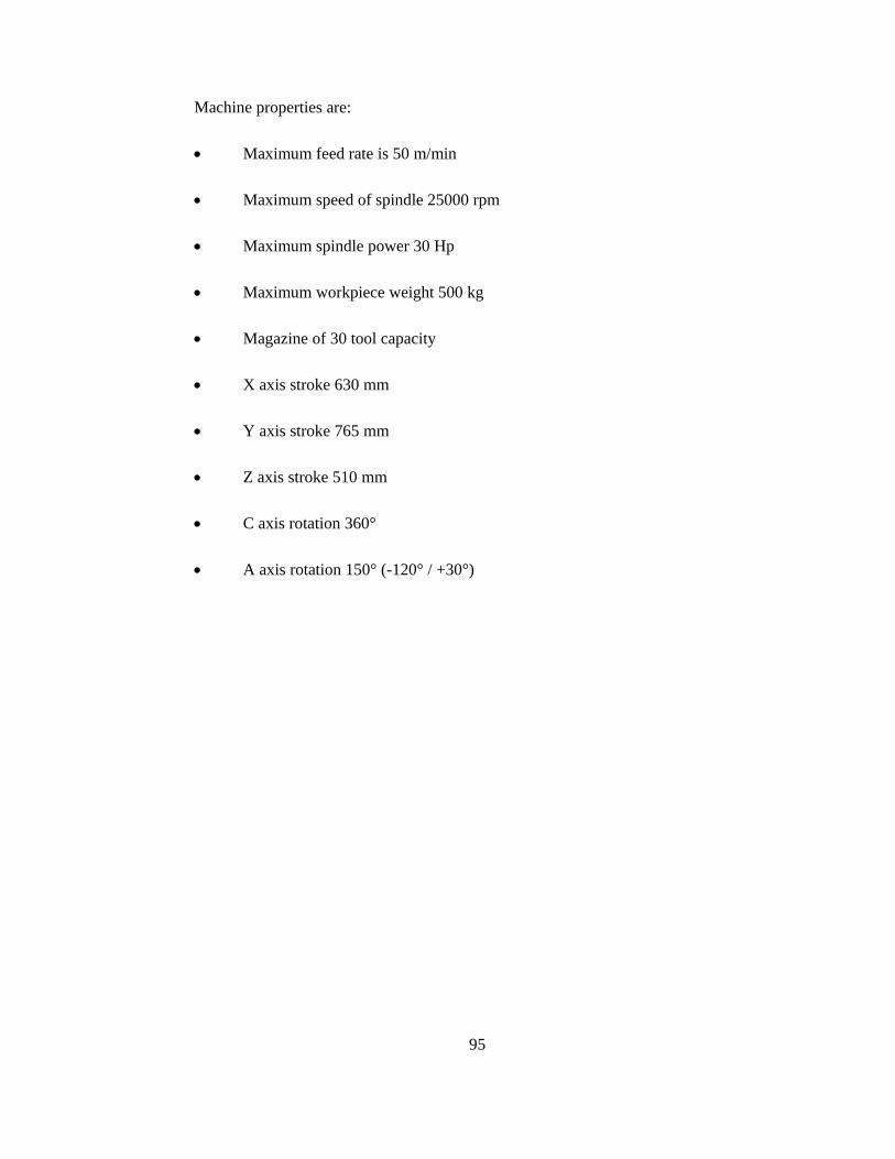
95
Machine properties are:
• Maximum feed rate is 50 m/min
• Maximum speed of spindle 25000 rpm
• Maximum spindle power 30 Hp
• Maximum workpiece weight 500 kg
• Magazine of 30 tool capacity
• X axis stroke 630 mm
• Y axis stroke 765 mm
• Z axis stroke 510 mm
• C axis rotation 360°
• A axis rotation 150° (-120° / +30°)
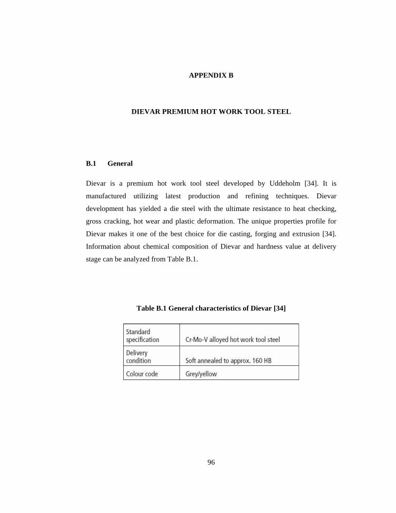
96
APPENDIX B
DIEVAR PREMIUM HOT WORK TOOL STEEL
B.1 General
Dievar is a premium hot work tool steel developed by Uddeholm [34]. It is
manufactured utilizing latest production and refining techniques. Dievar
development has yielded a die steel with the ultimate resistance to heat checking,
gross cracking, hot wear and plastic deformation. The unique properties profile for
Dievar makes it one of the best choice for die casting, forging and extrusion [34].
Information about chemical composition of Dievar and hardness value at delivery
stage can be analyzed from Table B.1.
Table B.1 General characteristics of Dievar [34]
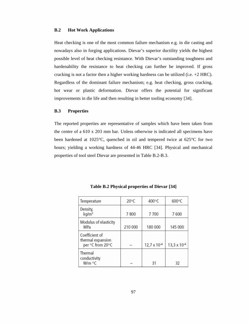
97
B.2 Hot Work Applications
Heat checking is one of the most common failure mechanism e.g. in die casting and
nowadays also in forging applications. Dievar’s superior ductility yields the highest
possible level of heat checking resistance. With Dievar’s outstanding toughness and
hardenability the resistance to heat checking can further be improved. If gross
cracking is not a factor then a higher working hardness can be utilized (i.e. +2 HRC).
Regardless of the dominant failure mechanism; e.g. heat checking, gross cracking,
hot wear or plastic deformation. Dievar offers the potential for significant
improvements in die life and then resulting in better tooling economy [34].
B.3 Properties
The reported properties are representative of samples which have been taken from
the centre of a 610 x 203 mm bar. Unless otherwise is indicated all specimens have
been hardened at 1025°C, quenched in oil and tempered twice at 625°C for two
hours; yielding a working hardness of 44-46 HRC [34]. Physical and mechanical
properties of tool steel Dievar are presented in Table B.2-B.3.
Table B.2 Physical properties of Dievar [34]
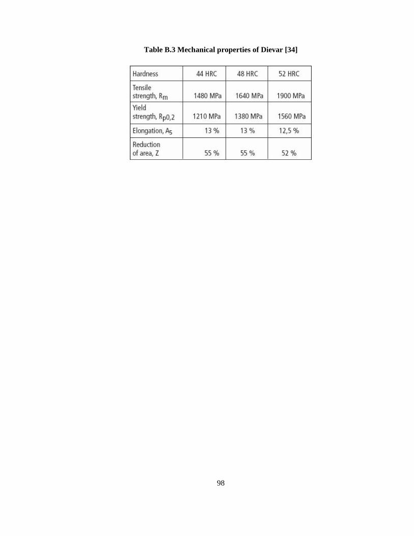
98
Table B.3 Mechanical properties of Dievar [34]
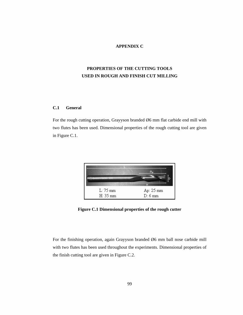
99
APPENDIX C
PROPERTIES OF THE CUTTING TOOLS
USED IN ROUGH AND FINISH CUT MILLING
C.1 General
For the rough cutting operation, Grayyson branded Ø6 mm flat carbide end mill with
two flutes has been used. Dimensional properties of the rough cutting tool are given
in Figure C.1.
Figure C.1 Dimensional properties of the rough cutter
For the finishing operation, again Grayyson branded Ø6 mm ball nose carbide mill
with two flutes has been used throughout the experiments. Dimensional properties of
the finish cutting tool are given in Figure C.2.
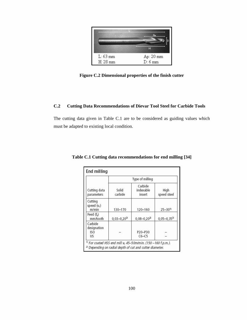
100
Figure C.2 Dimensional properties of the finish cutter
C.2 Cutting Data Recommendations of Dievar Tool Steel for Carbide Tools
The cutting data given in Table C.1 are to be considered as guiding values which
must be adapted to existing local condition.
Table C.1 Cutting data recommendations for end milling [34]
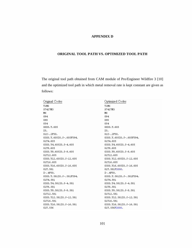
101
APPENDIX D
ORIGINAL TOOL PATH VS. OPTIMIZED TOOL PATH
The original tool path obtained from CAM module of Pro/Engineer Wildfire 3 [10]
and the optimized tool path in which metal removal rate is kept constant are given as
follows:
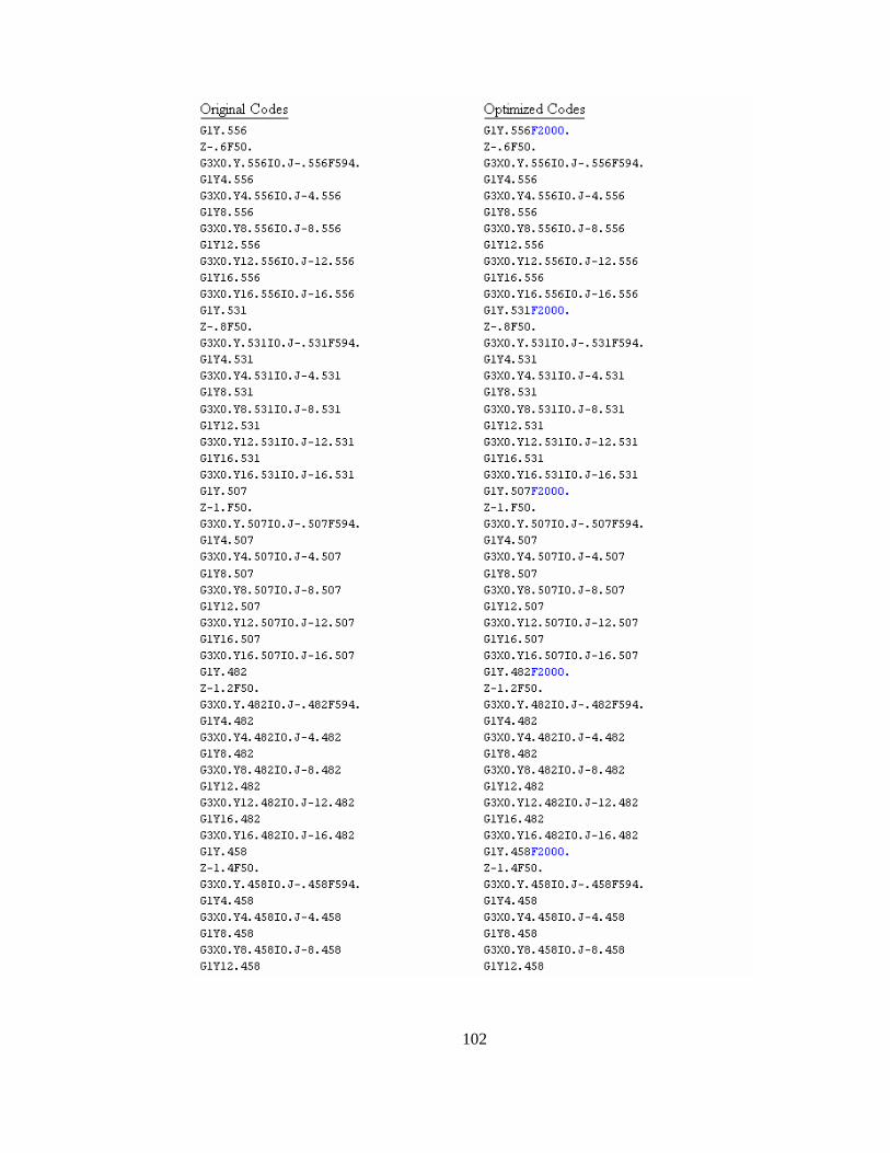
102
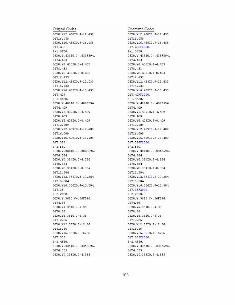
103
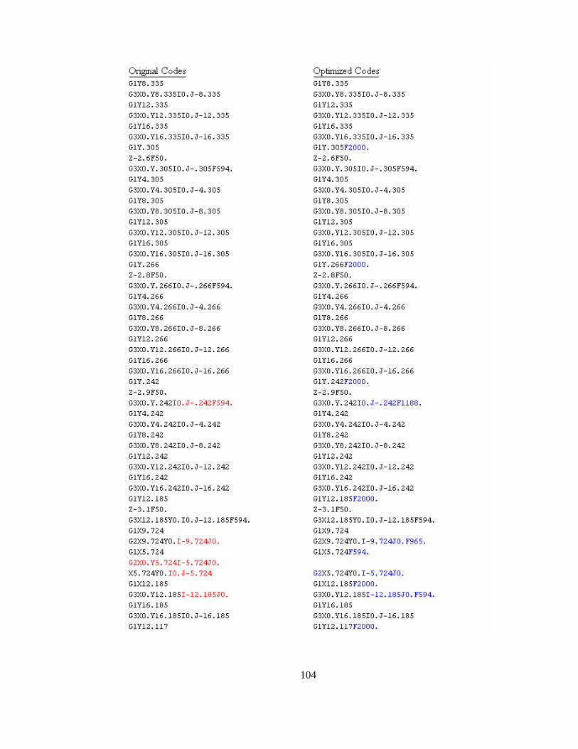
104
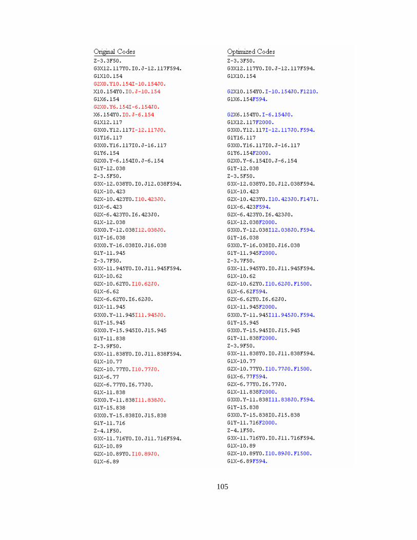
105
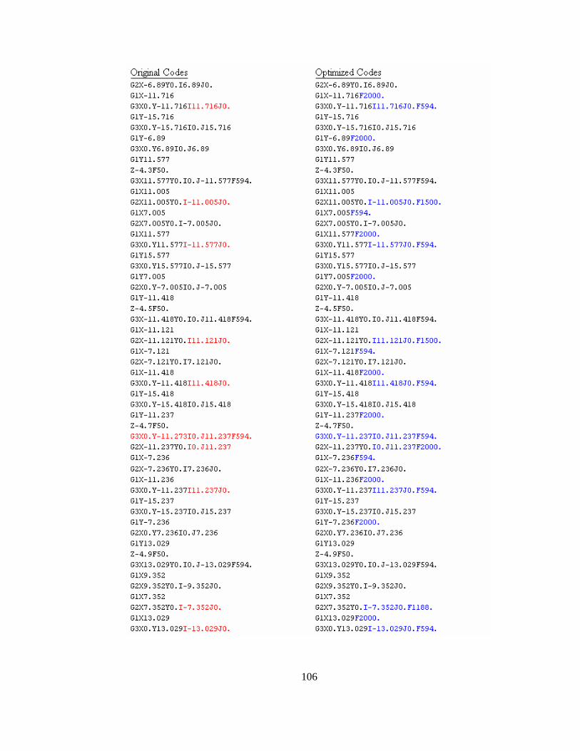
106
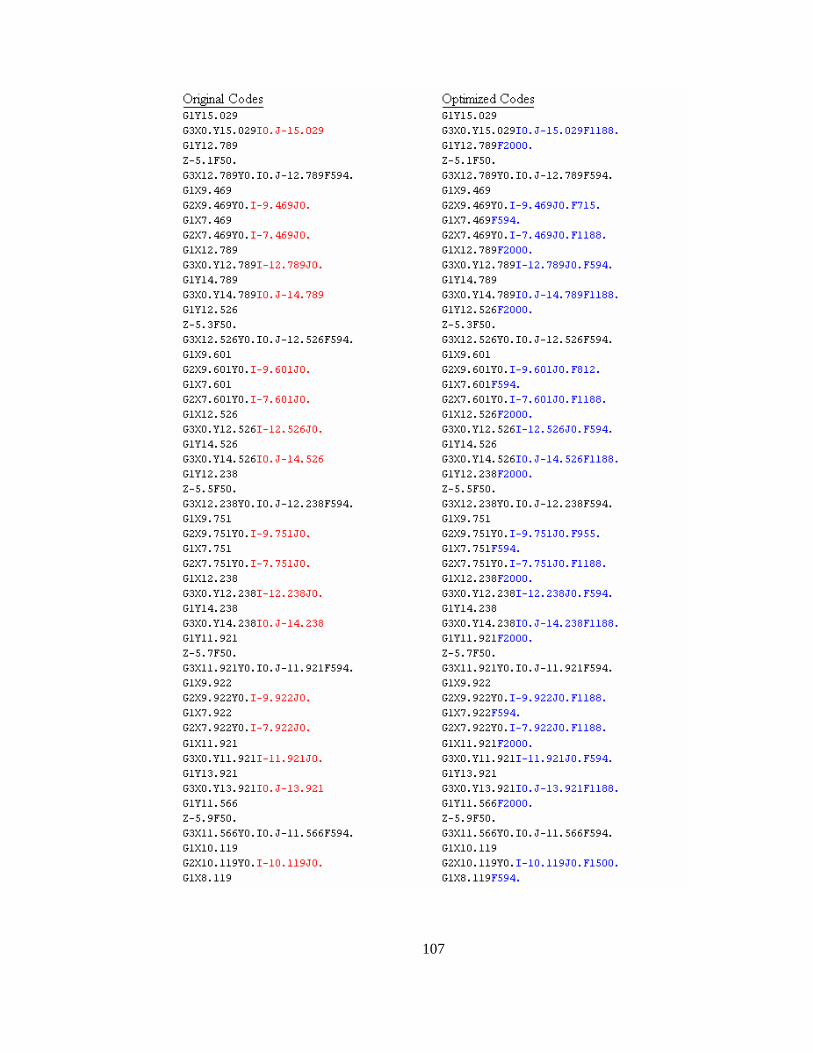
107
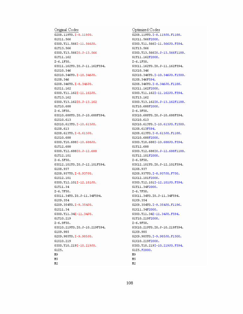
108
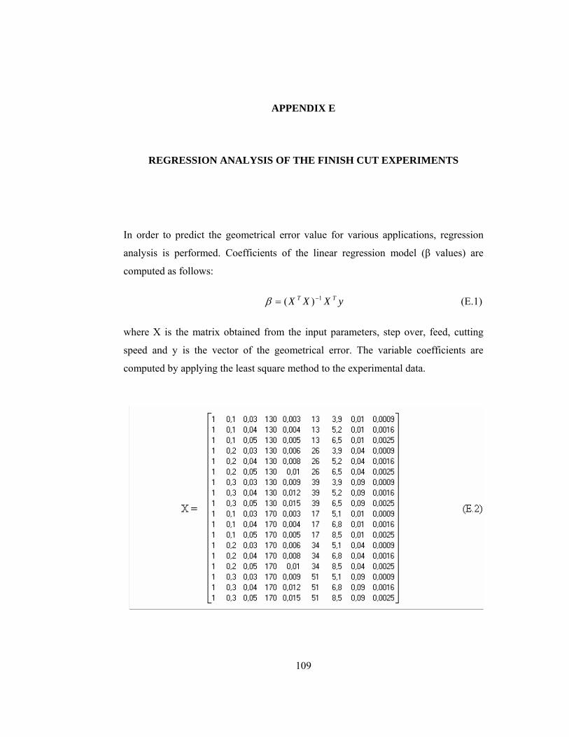
109
APPENDIX E
REGRESSION ANALYSIS OF THE FINISH CUT EXPERIMENTS
In order to predict the geometrical error value for various applications, regression
analysis is performed. Coefficients of the linear regression model (β values) are
computed as follows:
yXXX TT 1)( −=β (E.1)
where X is the matrix obtained from the input parameters, step over, feed, cutting
speed and y is the vector of the geometrical error. The variable coefficients are
computed by applying the least square method to the experimental data.
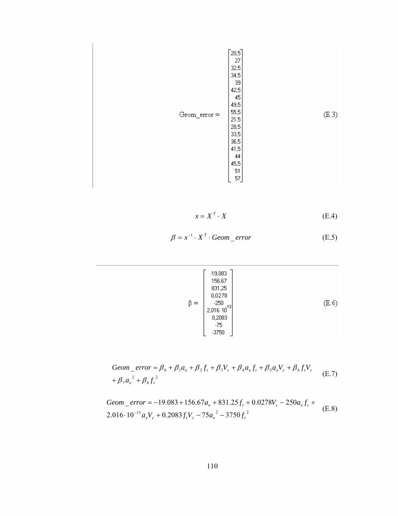
110
XXx T ⋅= (E.4)
errorGeomXx T _1 ⋅⋅= −β (E.5)
28
27
6543210_
te
ctcetecte
fa
VfVafaVfaerrorGeom
ββ
βββββββ
++
++++++= (E.7)
2213 3750752083.010016.2
2500278.025.83167.156083.19_
tectce
tecte
faVfVa
faVfaerrorGeom
−−+⋅
+−+++−=−
(E.8)


![Die forging - Metal Journal · Die forging The analysis of ... The production of elongated forgings with sharpened end on the roll -forging machine ... of calculation [20, 21] was](https://static.fdocuments.in/doc/165x107/5ad8f0677f8b9a3e578dffe8/die-forging-metal-forging-the-analysis-of-the-production-of-elongated-forgings.jpg)