Curves, a Tale of Beauty,

Chaos, and Science

Curves from Euler to Schrödinger

Nilton Aranda Neto

26th March 2021

2

Curves, a Tale of Beauty, Chaos, and Science: Curves from Euler to Schrödinger

“Any curve that has a name has a story”

– Julian Havil

Curves are everywhere. Some we have created; others nature has

constructed for us. We are all born with an understanding instinct for geometry

and the shapes that are so familiar to us all. From arches on bridges to the

parabola a ball traces as it is thrown into a basketball hoop; it may never be

truly apparent how curves have been so fundamentally ingrained within our

lives. Many curves you will see on a daily basis, perhaps in buildings or

construction, while useful are usually purely functional. However beautiful,

some curves have no uses, no way of being manipulated for real-life applications

and yet there are some on the brink of science that are not only functional in

holding together matter but perhaps will show you the beauty of maths within

science.

Firstly, what is a curve? The answer is fairly intuitive, take a moving

object and trace its course on a two-dimensional or even three-dimensional axis

and you will be left with a curve. Fundamentally, it is also possible to conceive

3

that a function producing a straight line e.g., 𝑓(𝑥) = 𝑥, is also a curve but just of

a lower order. It is in this way that we can say the definition of a curve is ‘the

image of an interval to a topological space by a continuous function’. You have

probably already encountered the most basic class of curve, algebraic curves.

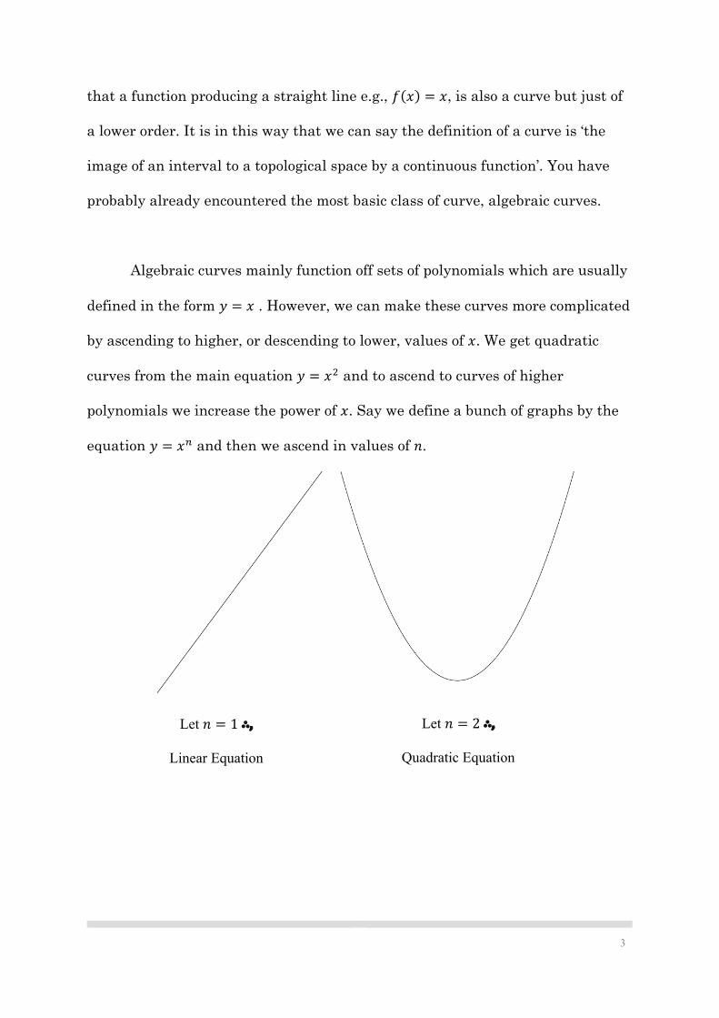
Algebraic curves mainly function off sets of polynomials which are usually

defined in the form 𝑦 = 𝑥 . However, we can make these curves more complicated

by ascending to higher, or descending to lower, values of 𝑥. We get quadratic

curves from the main equation 𝑦 = 𝑥! and to ascend to curves of higher

polynomials we increase the power of 𝑥. Say we define a bunch of graphs by the

equation 𝑦 = 𝑥" and then we ascend in values of 𝑛.

Let 𝑛 = 1∴,

Linear Equation

Linear equation

Let 𝑛 = 2∴,

Quadratic Equation

Linear equation

4

I’m sure you’ve noticed that if you look at the ends of these graphs to the

right and left they all tend either upwards or downwards. For the quadratic

graph for example or parabola it can be said as you move along the 𝑥axis (either

right or left horizontally) that the values for thegradient tend towards infinity,

(positive infinity or negative, depending on which side of the axis you go to). This

in essence is what makes a curve differentiable. By differentiating the equation

or function of a curve we can track its gradient as a tangent to a specific value of

𝑥 in the curve. This is the main basis of differentiation in calculus.

This brings us to further types of curves in which we need to understand

how to distinguish. Some curves cannot be differentiated i.e., we cannot work out

their gradient algebraically at specific points along the axis. Many of these

curves are incredibly complex as they often have fractal properties (they repeat

Let 𝑛 = 3∴,

Cubic Equation

Linear equation

Let 𝑛 = 4∴,

Quartic Equation

Linear equation

5

or iterate in a sequence as we zoom in on them) or they can be what are called

space filling curves, as they occupy the whole two-dimensional axis.

An example of one of these curves would be the Weierstrass function:

Conceived by Weierstrass in 1872 it completely redefined ideas of

graphical smoothness and what was possible with functions on a cartesian plane.

Looking back at the history, it is clear that this would have been one of the first

fractals ever discovered and studied. What makes this curve so special is that it

cannot be differentiated at any point. Interestingly enough, no matter how far you zoom

in on a segment of this curve it will never stop changing and this is why we can call it a

fractal curve as not only can we not differentiate it we are not able to see a base state for this

curve as it repeats infinitely. Take any polynomial curve for example and zoom in on a point,

eventually having zoomed in enough the curve will just appear to look like a straight line

The Weierstrass function with segments of the graph

zoomed in.

6

since you have zoomed in so far it is indeterminate to a line with a constant gradient. Now

take the Weierstrass function and zoom in, there will be no point that even tends towards

becoming a straight line, in this sense we can say the function will not be monotone, this is

why we can say the curve is ‘continuous everywhere but differentiable nowhere’. The

Weierstrass function also has many applications in computing for instance as being able to

compute different levels of zoom within a certain time can be used as a performance metric

for the speed of software or hardware.

There are other curves with very functional uses especially in architecture and

engineering, take the Euler Spiral for instance which was first introduced to me through one

of my favorite books Curves for the Mathematically Curious:

7

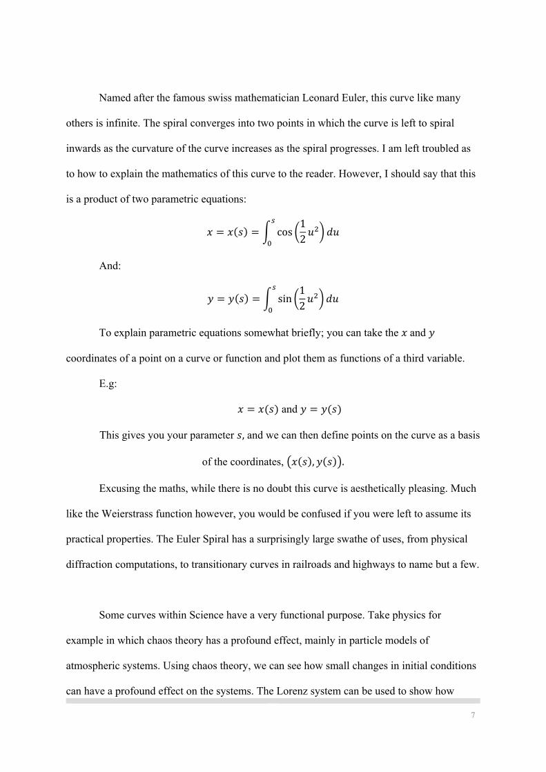
Named after the famous swiss mathematician Leonard Euler, this curve like many

others is infinite. The spiral converges into two points in which the curve is left to spiral

inwards as the curvature of the curve increases as the spiral progresses. I am left troubled as

to how to explain the mathematics of this curve to the reader. However, I should say that this

is a product of two parametric equations:

𝑥 = 𝑥(𝑠) = 0 cos 412𝑢

!6 𝑑𝑢#

$

And:

𝑦 = 𝑦(𝑠) = 0 sin 412𝑢

!6𝑑𝑢#

$

To explain parametric equations somewhat briefly; you can take the 𝑥and 𝑦

coordinates of a point on a curve or function and plot them as functions of a third variable.

E.g:

𝑥 = 𝑥(𝑠) and 𝑦 = 𝑦(𝑠)

This gives you your parameter 𝑠, and we can then define points on the curve as a basis

of the coordinates, :𝑥(𝑠), 𝑦(𝑠);.

Excusing the maths, while there is no doubt this curve is aesthetically pleasing. Much

like the Weierstrass function however, you would be confused if you were left to assume its

practical properties. The Euler Spiral has a surprisingly large swathe of uses, from physical

diffraction computations, to transitionary curves in railroads and highways to name but a few.

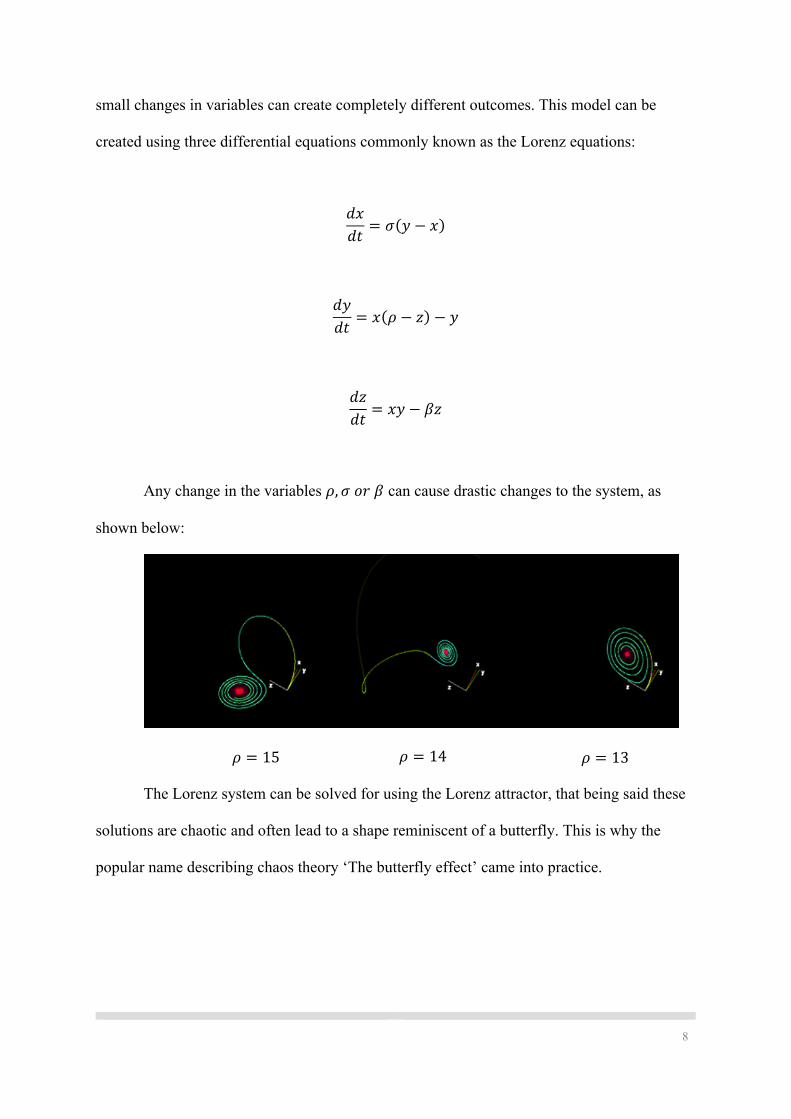
Some curves within Science have a very functional purpose. Take physics for

example in which chaos theory has a profound effect, mainly in particle models of

atmospheric systems. Using chaos theory, we can see how small changes in initial conditions

can have a profound effect on the systems. The Lorenz system can be used to show how

8

small changes in variables can create completely different outcomes. This model can be

created using three differential equations commonly known as the Lorenz equations:

𝑑𝑥𝑑𝑡 = 𝜎(𝑦 − 𝑥)

𝑑𝑦𝑑𝑡 = 𝑥(𝜌 − 𝑧) − 𝑦

𝑑𝑧𝑑𝑡 = 𝑥𝑦 − 𝛽𝑧

Any change in the variables 𝜌, 𝜎𝑜𝑟𝛽 can cause drastic changes to the system, as

shown below:

The Lorenz system can be solved for using the Lorenz attractor, that being said these

solutions are chaotic and often lead to a shape reminiscent of a butterfly. This is why the

popular name describing chaos theory ‘The butterfly effect’ came into practice.

𝜌 = 15 𝜌 = 14 𝜌 = 13

9

Going beyond chaos theory, however, curves have fundamentally changed how

physicists and chemists perceive matter. This is particularly present in quantum mechanics

where wave equations and functions are found plentifully. The discovery of the wave

function and the main basis for quantum theory is all thanks to the ingenuity of Schrödinger.

Many physicists and chemists are particularly fond of the beauty of mathematical functions

which describe certain particles, especially electrons. We can successfully describe their

properties using Schrödinger’s equations. The Bohr model of the atom is the one most people

are familiar with, a central core nucleus which is shared by protons and neutrons with

As you can see this Lorenz Attractor solution to a

Lorenz system is very familiar to the shape of a butterfly

10

electrons orbiting around like planets and moons. However, Schrödinger was able to

fundamentally prove that this was not the case. The wave function is made up of two

fundamental parts. Schrödinger’s Equation and the wavefunction itself:

This is the Schrödinger’s equation, in which 𝜓 (the wavefunction) is a direct solution.

This wavefunction was first formulated over to work out the shapes of the electron orbitals of

hydrogen of which have been calculated precisely and can be described by the equation

below:

𝜓!"#(𝑟, 𝜗, 𝜑) = )*2𝑛𝑎$

.% (𝑛 − 𝑙 − 1)!2𝑛[(𝑛 + 𝑙)!]

𝑒&'(𝜌"𝐿!&"&)*"+) (𝜌) ∗ 𝑌"#(𝜗, 𝜑)

Interestingly enough, the wave function is plotted three-dimensionally using a

spherical polar coordinate system. In this system 𝑟is the radius, 𝜃the colatitude, and 𝜙 is the

azimuth.

11

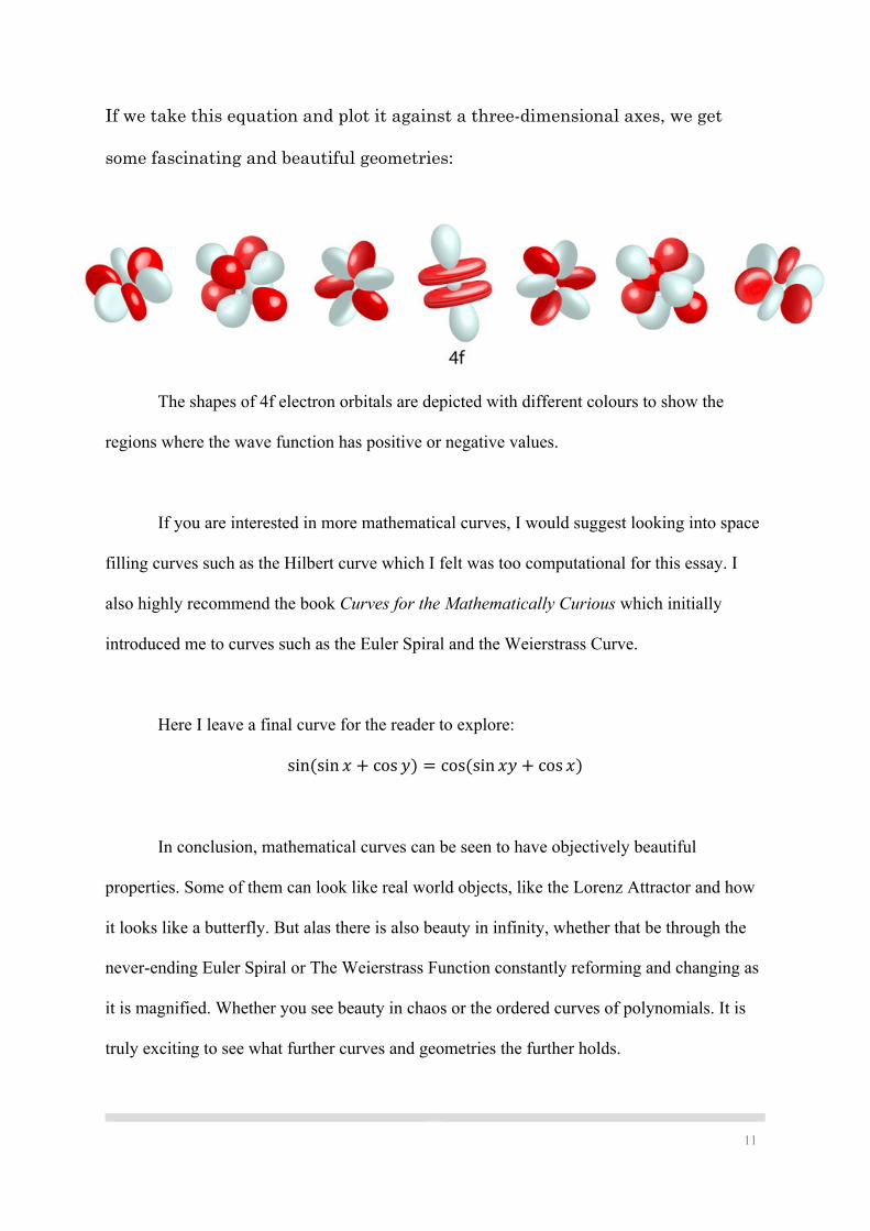
If we take this equation and plot it against a three-dimensional axes, we get

some fascinating and beautiful geometries:

The shapes of 4f electron orbitals are depicted with different colours to show the

regions where the wave function has positive or negative values.

If you are interested in more mathematical curves, I would suggest looking into space

filling curves such as the Hilbert curve which I felt was too computational for this essay. I

also highly recommend the book Curves for the Mathematically Curious which initially

introduced me to curves such as the Euler Spiral and the Weierstrass Curve.

Here I leave a final curve for the reader to explore:

sin(sin 𝑥 + cos 𝑦) = cos(sin 𝑥𝑦 + cos 𝑥)

In conclusion, mathematical curves can be seen to have objectively beautiful

properties. Some of them can look like real world objects, like the Lorenz Attractor and how

it looks like a butterfly. But alas there is also beauty in infinity, whether that be through the

never-ending Euler Spiral or The Weierstrass Function constantly reforming and changing as

it is magnified. Whether you see beauty in chaos or the ordered curves of polynomials. It is

truly exciting to see what further curves and geometries the further holds.

12

Sources List:

Atkins, P.W. (2010). Shriver & Atkins’ Inorganic Chemistry. Oxford ; New York: Oxford University Press.

Havil, J. (2019). Curves for the Mathematically Curious : an anthology of the unpredictable, historical, beautiful and romantic. Princeton, New Jersey ; Oxford: Princeton University Press.

Numberphile and Fry, H. (2018). A Strange Map Projection (Euler Spiral) - Numberphile. [online] www.youtube.com. Available at: https://www.youtube.com/watch?v=D3tdW9l1690 [Accessed 26 Mar. 2021].

Star, Z. (2020). Curves We (mostly) don’t Learn in High School (and applications). [online] www.youtube.com. Available at: https://www.youtube.com/watch?v=3izFMB91K_Q&t=330s [Accessed 26 Mar. 2021].

Wikipedia. (2019). Chaos Theory. [online] Available at: https://en.wikipedia.org/wiki/Chaos_Theory.

Wikipedia. (2020a). Lorenz System. [online] Available at: https://en.wikipedia.org/wiki/Lorenz_system.

Wikipedia. (2020b). Space-filling Curve. [online] Available at: https://en.wikipedia.org/wiki/Space-filling_curve.

Wikipedia. (2021a). Euler Spiral. [online] Available at: https://en.wikipedia.org/wiki/Euler_spiral#:~:text=Symbols%20%20%20R%20%20%20Radius%20of.

Wikipedia. (2021b). Hydrogen Atom. [online] Available at: https://en.wikipedia.org/wiki/Hydrogen_atom#Wavefunction [Accessed 26 Mar. 2021].

Wikipedia. (2021c). Weierstrass Function. [online] Available at: https://en.wikipedia.org/wiki/Weierstrass_function.

Winter, M. (n.d.). The Orbitron: a Gallery of Atomic Orbitals on the WWW. [online] winter.group.shef.ac.uk. Available at: https://winter.group.shef.ac.uk/orbitron/ [Accessed 26 Mar. 2021].