Curve Fitting – General - NCSS · Curve Fitting – General Introduction Curve fitting refers to...

NCSS Statistical Software NCSS.com

351-1 © NCSS, LLC. All Rights Reserved.

Chapter 351

Curve Fitting – General Introduction Curve fitting refers to finding an appropriate mathematical model that expresses the relationship between a dependent variable Y and a single independent variable X and estimating the values of its parameters using nonlinear regression. An introduction to curve fitting and nonlinear regression can be found in the chapter entitled Curve Fitting, so these details will not repeated here. Here are some examples of the curve fitting that can be accomplished with this procedure.

This program is general purpose curve fitting procedure providing many new technologies that have not been easily available. It is preprogrammed to fit over forty common mathematical models including growth models like linear-growth and Michaelis-Menten. It also fits many approximating models such as regular polynomials, piecewise polynomials and polynomial ratios. In addition to these preprogrammed models, it also fits models that you write yourself.

This routine includes several innovative features. First, it can fit curves to several batches of data simultaneously. Second, it compares fitted models across groups using graphics and numerical tests such as an approximate F-test for curve coincidence and a computer-intensive randomization test that compares curve coincidence and individual parameter values. Third, this routine computes bootstrap confidence intervals for parameter values, predicted means, and predicted values using the latest computer-intensive bootstrapping technology.

http://www.ncss.com/

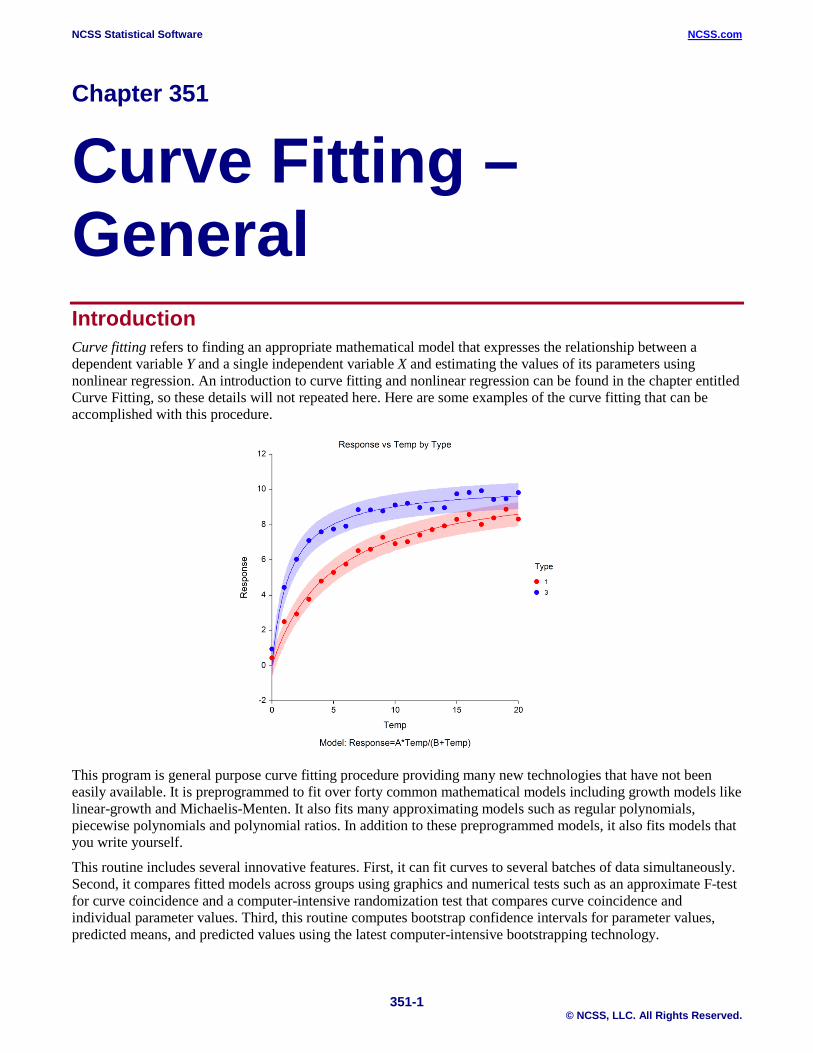
NCSS Statistical Software NCSS.com Curve Fitting – General


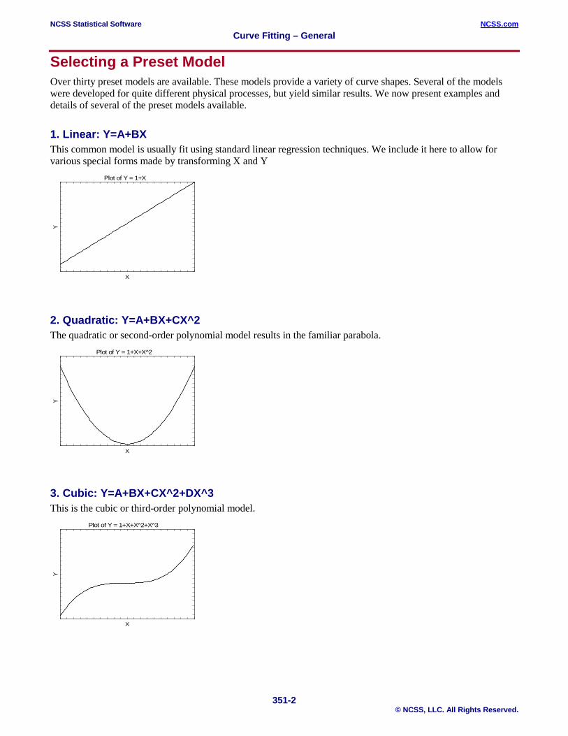
Selecting a Preset Model Over thirty preset models are available. These models provide a variety of curve shapes. Several of the models were developed for quite different physical processes, but yield similar results. We now present examples and details of several of the preset models available.

1. Linear: Y=A+BX This common model is usually fit using standard linear regression techniques. We include it here to allow for various special forms made by transforming X and Y

2. Quadratic: Y=A+BX+CX^2 The quadratic or second-order polynomial model results in the familiar parabola.

3. Cubic: Y=A+BX+CX^2+DX^3 This is the cubic or third-order polynomial model.

Plot of Y = 1+X

X

Y

Plot of Y = 1+X+X^2

X

Y

Plot of Y = 1+X+X^2+X^3

X

Y




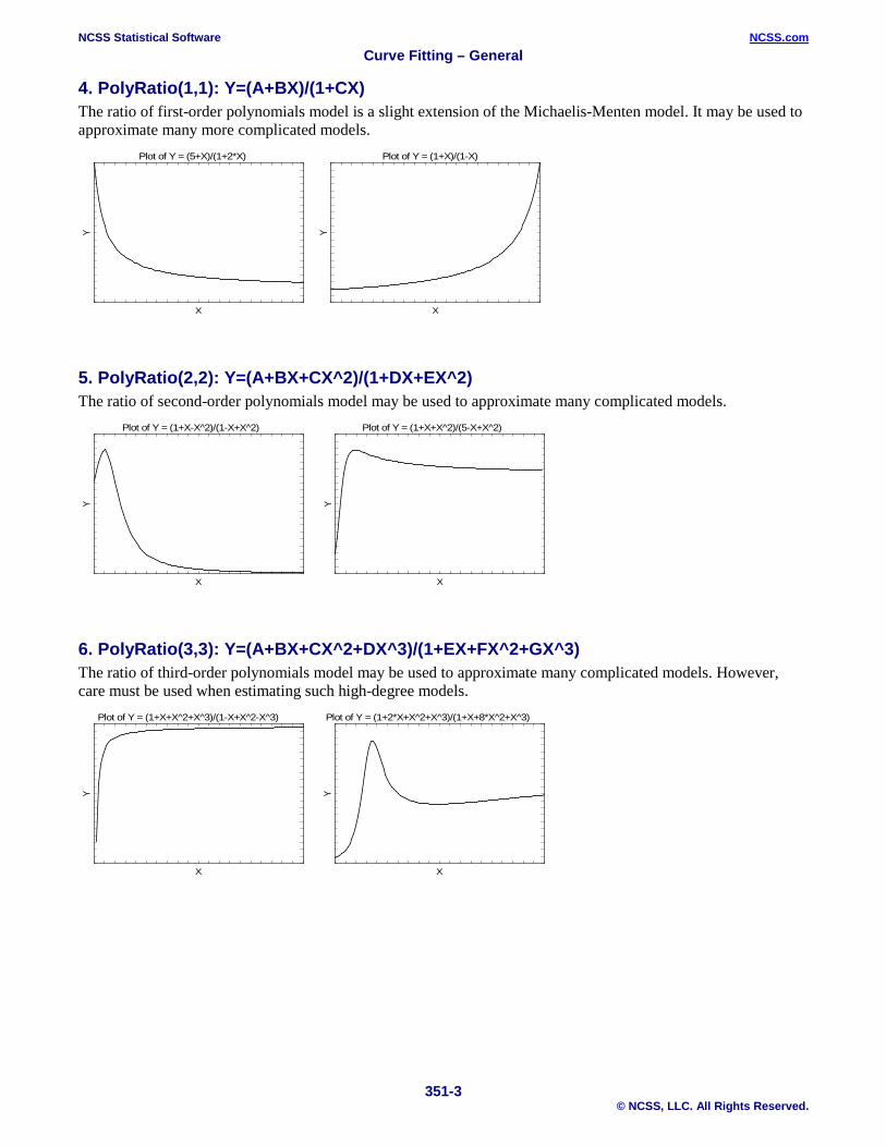
4. PolyRatio(1,1): Y=(A+BX)/(1+CX) The ratio of first-order polynomials model is a slight extension of the Michaelis-Menten model. It may be used to approximate many more complicated models.

5. PolyRatio(2,2): Y=(A+BX+CX^2)/(1+DX+EX^2) The ratio of second-order polynomials model may be used to approximate many complicated models.

6. PolyRatio(3,3): Y=(A+BX+CX^2+DX^3)/(1+EX+FX^2+GX^3) The ratio of third-order polynomials model may be used to approximate many complicated models. However, care must be used when estimating such high-degree models.

Plot of Y = (5+X)/(1+2*X)

X

Y

Plot of Y = (1+X)/(1-X)

XY

Plot of Y = (1+X-X^2)/(1-X+X^2)

X

Y

Plot of Y = (1+X+X^2)/(5-X+X^2)

X

Y

Plot of Y = (1+X+X^2+X^3)/(1-X+X^2-X^3)

X

Y

Plot of Y = (1+2*X+X^2+X^3)/(1+X+8*X^2+X^3)

X

Y




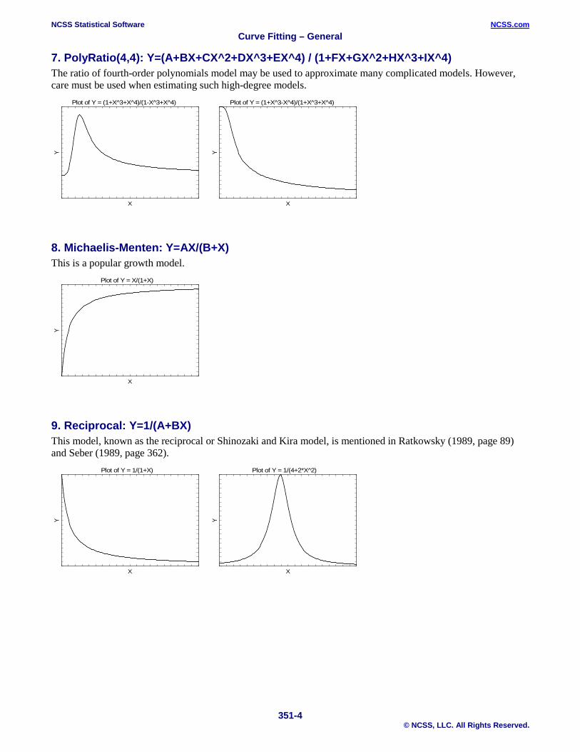
7. PolyRatio(4,4): Y=(A+BX+CX^2+DX^3+EX^4) / (1+FX+GX^2+HX^3+IX^4) The ratio of fourth-order polynomials model may be used to approximate many complicated models. However, care must be used when estimating such high-degree models.

8. Michaelis-Menten: Y=AX/(B+X) This is a popular growth model.

9. Reciprocal: Y=1/(A+BX) This model, known as the reciprocal or Shinozaki and Kira model, is mentioned in Ratkowsky (1989, page 89) and Seber (1989, page 362).

Plot of Y = (1+X^3+X^4)/(1-X^3+X^4)

X

Y

Plot of Y = (1+X^3-X^4)/(1+X^3+X^4)

X

Y

Plot of Y = X/(1+X)

X

Y

Plot of Y = 1/(1+X)

X

Y

Plot of Y = 1/(4+2*X^2)

X

Y




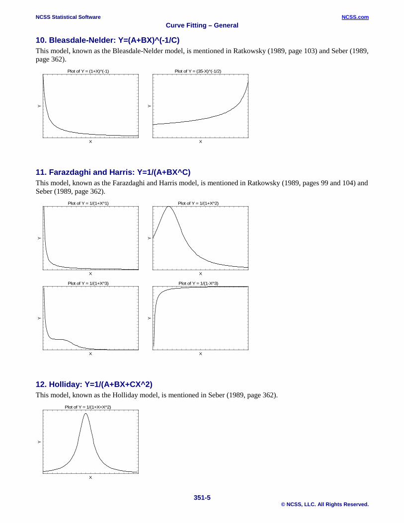
10. Bleasdale-Nelder: Y=(A+BX)^(-1/C) This model, known as the Bleasdale-Nelder model, is mentioned in Ratkowsky (1989, page 103) and Seber (1989, page 362).

11. Farazdaghi and Harris: Y=1/(A+BX^C) This model, known as the Farazdaghi and Harris model, is mentioned in Ratkowsky (1989, pages 99 and 104) and Seber (1989, page 362).

12. Holliday: Y=1/(A+BX+CX^2) This model, known as the Holliday model, is mentioned in Seber (1989, page 362).

Plot of Y = (1+X)^(-1)

X

Y

Plot of Y = (35-X)^(-1/2)

X

Y

Plot of Y = 1/(1+X^1)

X

Y

Plot of Y = 1/(1+X^2)

X

Y

Plot of Y = 1/(1+X^3)

X

Y

Plot of Y = 1/(1-X^3)

X

Y

Plot of Y = 1/(1+X+X^2)

X

Y




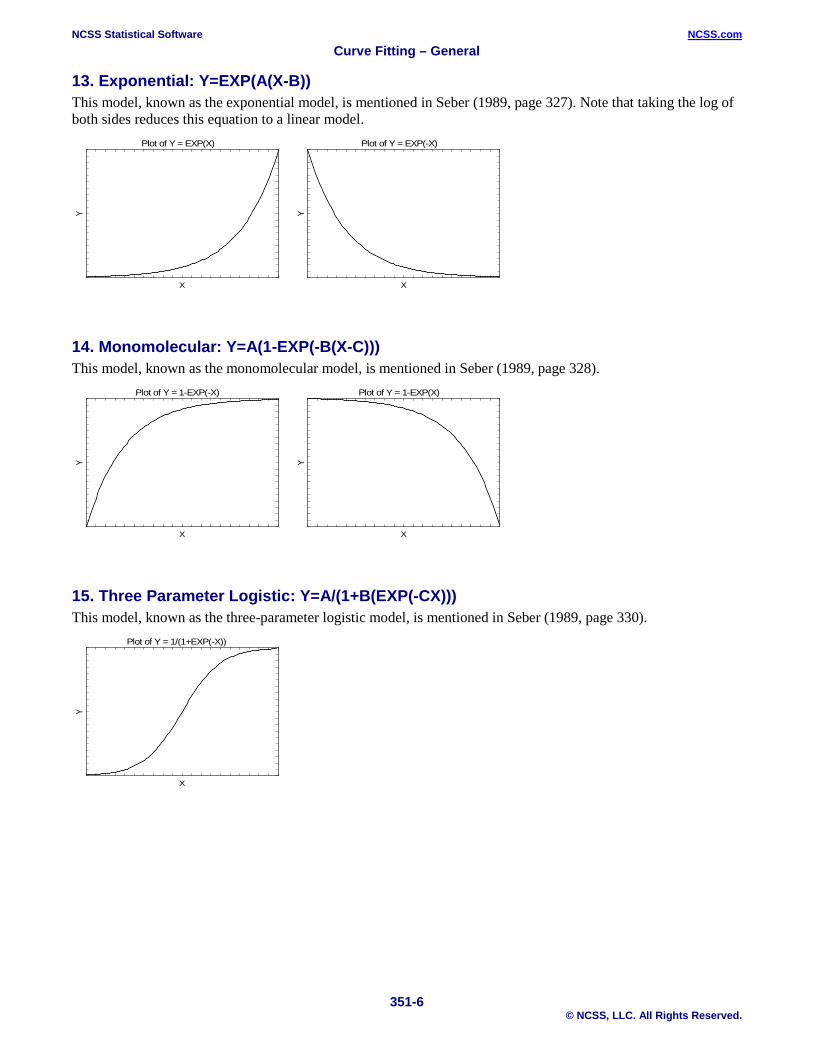
13. Exponential: Y=EXP(A(X-B)) This model, known as the exponential model, is mentioned in Seber (1989, page 327). Note that taking the log of both sides reduces this equation to a linear model.

14. Monomolecular: Y=A(1-EXP(-B(X-C))) This model, known as the monomolecular model, is mentioned in Seber (1989, page 328).

15. Three Parameter Logistic: Y=A/(1+B(EXP(-CX))) This model, known as the three-parameter logistic model, is mentioned in Seber (1989, page 330).

Plot of Y = EXP(X)

X

Y

Plot of Y = EXP(-X)

X

Y

Plot of Y = 1-EXP(-X)

X

Y

Plot of Y = 1-EXP(X)

X

Y

Plot of Y = 1/(1+EXP(-X))

X

Y




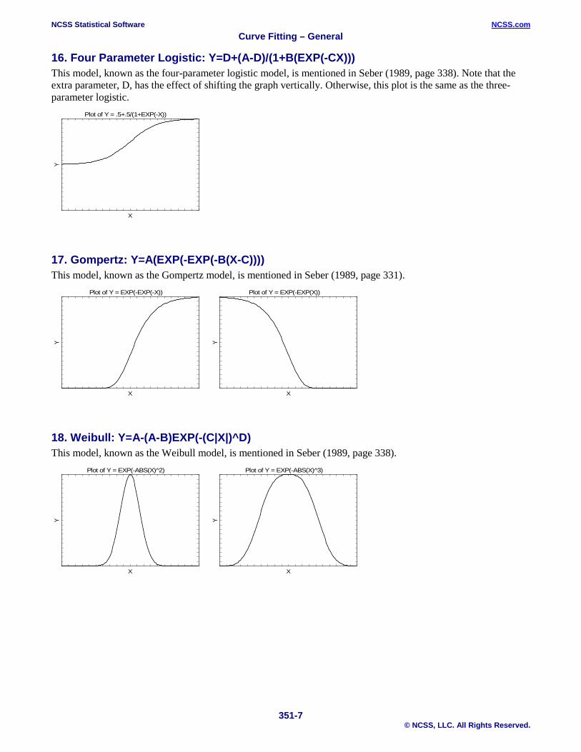
16. Four Parameter Logistic: Y=D+(A-D)/(1+B(EXP(-CX))) This model, known as the four-parameter logistic model, is mentioned in Seber (1989, page 338). Note that the extra parameter, D, has the effect of shifting the graph vertically. Otherwise, this plot is the same as the three-parameter logistic.

17. Gompertz: Y=A(EXP(-EXP(-B(X-C)))) This model, known as the Gompertz model, is mentioned in Seber (1989, page 331).

18. Weibull: Y=A-(A-B)EXP(-(C|X|)^D) This model, known as the Weibull model, is mentioned in Seber (1989, page 338).

Plot of Y = .5+.5/(1+EXP(-X))

X

Y

Plot of Y = EXP(-EXP(-X))

X

Y

Plot of Y = EXP(-EXP(X))

X

Y

Plot of Y = EXP(-ABS(X)^2)

X

Y

Plot of Y = EXP(-ABS(X)^3)

X

Y




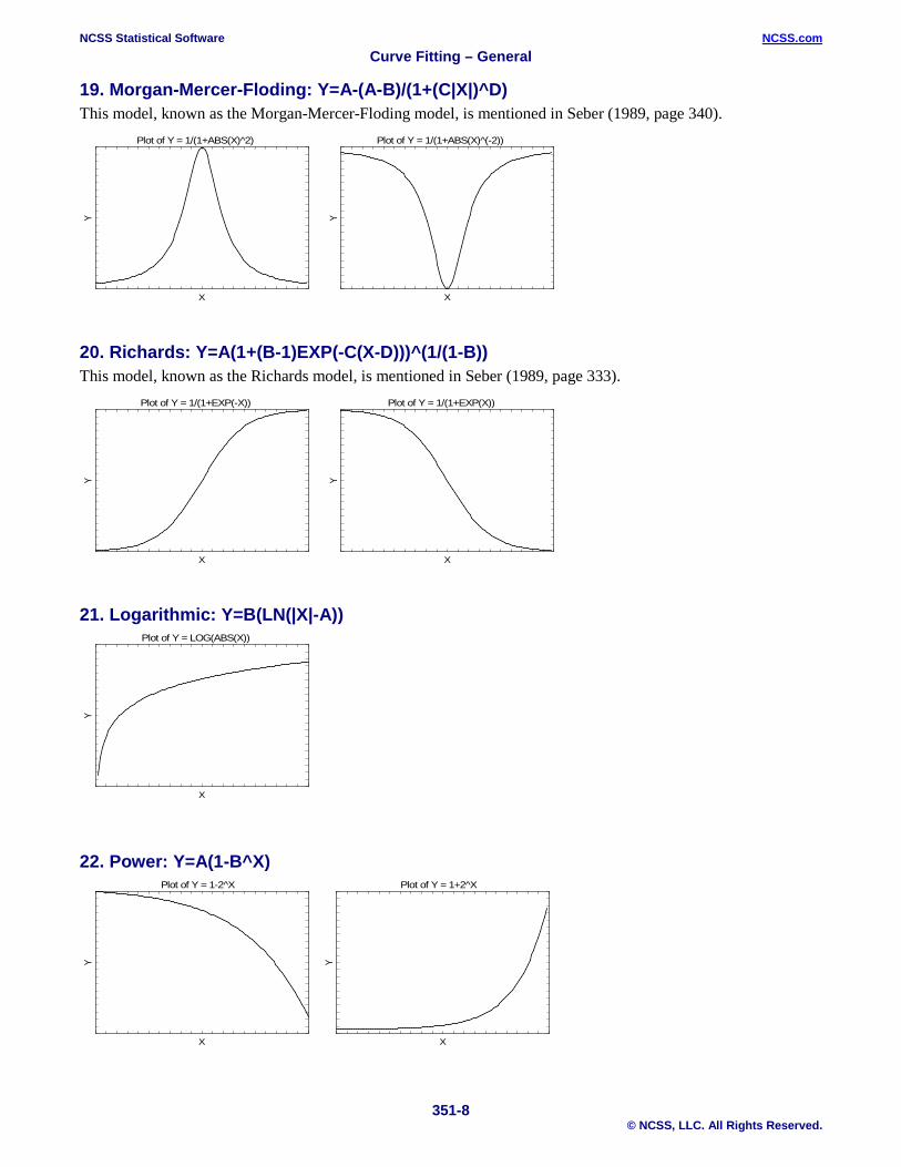
19. Morgan-Mercer-Floding: Y=A-(A-B)/(1+(C|X|)^D) This model, known as the Morgan-Mercer-Floding model, is mentioned in Seber (1989, page 340).

20. Richards: Y=A(1+(B-1)EXP(-C(X-D)))^(1/(1-B)) This model, known as the Richards model, is mentioned in Seber (1989, page 333).

21. Logarithmic: Y=B(LN(|X|-A))

22. Power: Y=A(1-B^X)

Plot of Y = 1/(1+ABS(X)^2)

X

Y

Plot of Y = 1/(1+ABS(X)^(-2))

X

Y

Plot of Y = 1/(1+EXP(-X))

X

Y

Plot of Y = 1/(1+EXP(X))

X

Y

Plot of Y = LOG(ABS(X))

X

Y

Plot of Y = 1-2^X

X

Y

Plot of Y = 1+2^X

X

Y




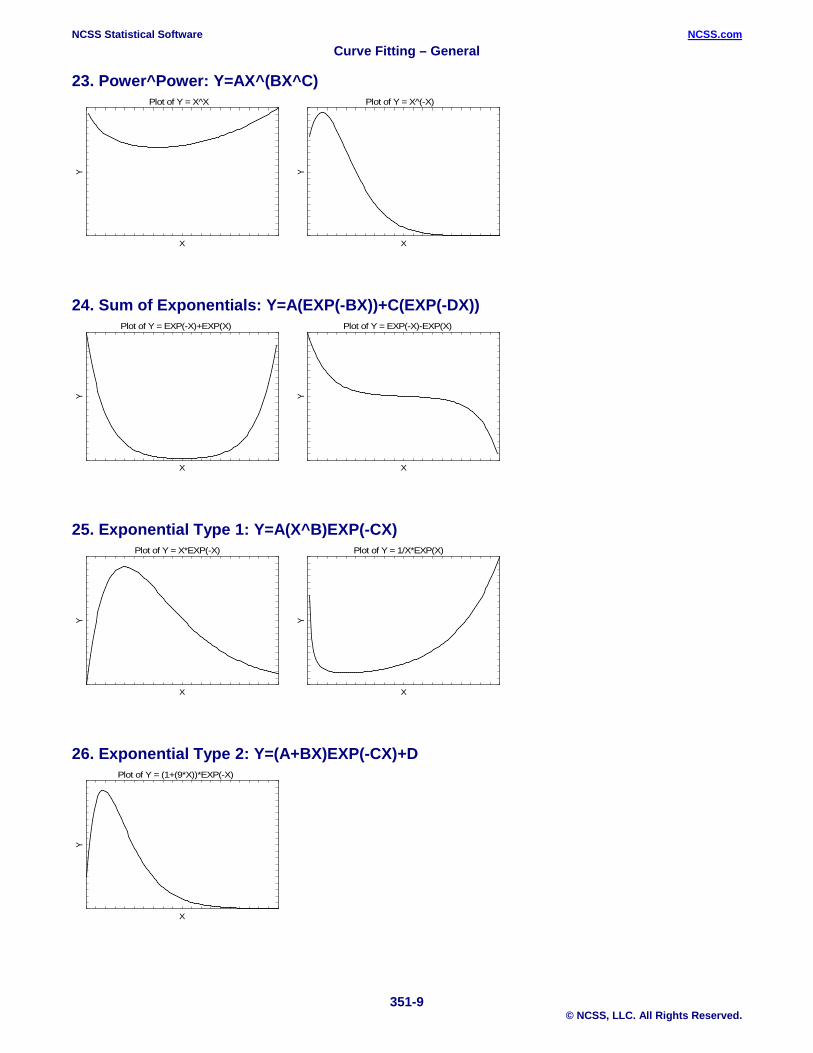
23. Power^Power: Y=AX^(BX^C)

24. Sum of Exponentials: Y=A(EXP(-BX))+C(EXP(-DX))

25. Exponential Type 1: Y=A(X^B)EXP(-CX)

26. Exponential Type 2: Y=(A+BX)EXP(-CX)+D

Plot of Y = X^X

X

Y

Plot of Y = X^(-X)

X

Y

Plot of Y = EXP(-X)+EXP(X)

X

Y

Plot of Y = EXP(-X)-EXP(X)

X

Y

Plot of Y = X*EXP(-X)

X

Y

Plot of Y = 1/X*EXP(X)

X

Y

Plot of Y = (1+(9*X))*EXP(-X)

X

Y




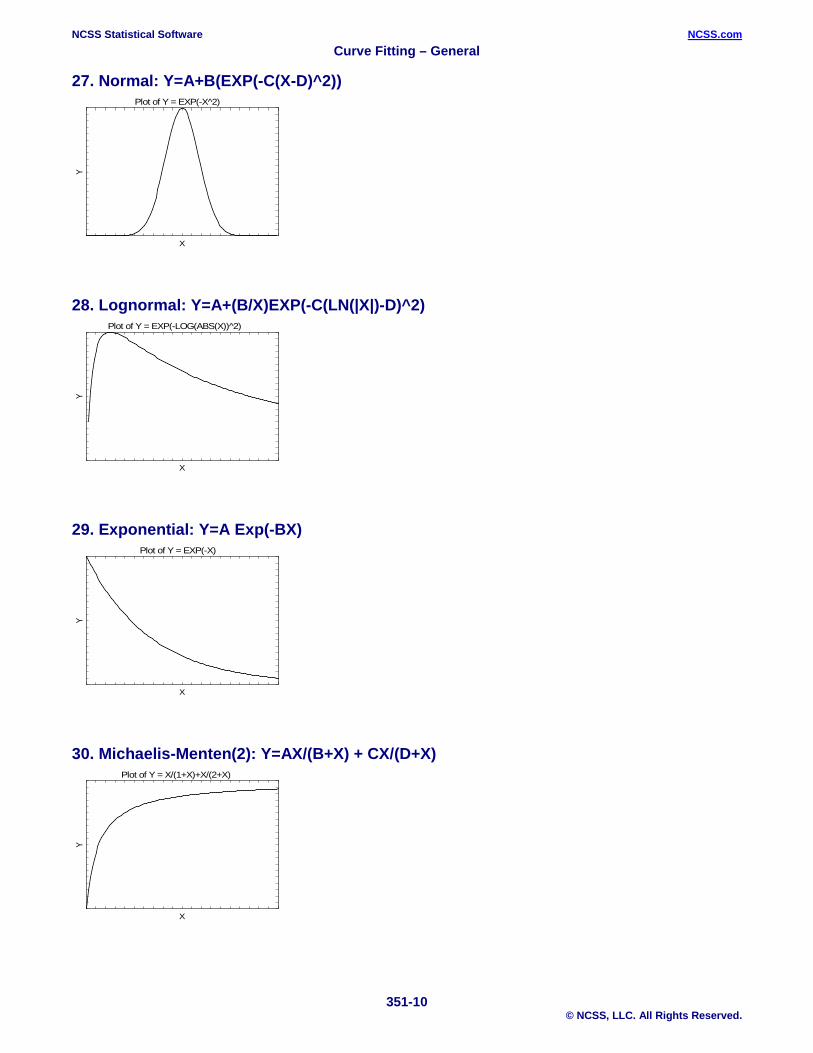
27. Normal: Y=A+B(EXP(-C(X-D)^2))

28. Lognormal: Y=A+(B/X)EXP(-C(LN(|X|)-D)^2)

29. Exponential: Y=A Exp(-BX)

30. Michaelis-Menten(2): Y=AX/(B+X) + CX/(D+X)

Plot of Y = EXP(-X^2)

X

Y

Plot of Y = EXP(-LOG(ABS(X))^2)

X

Y

Plot of Y = EXP(-X)

X

Y

Plot of Y = X/(1+X)+X/(2+X)

X

Y




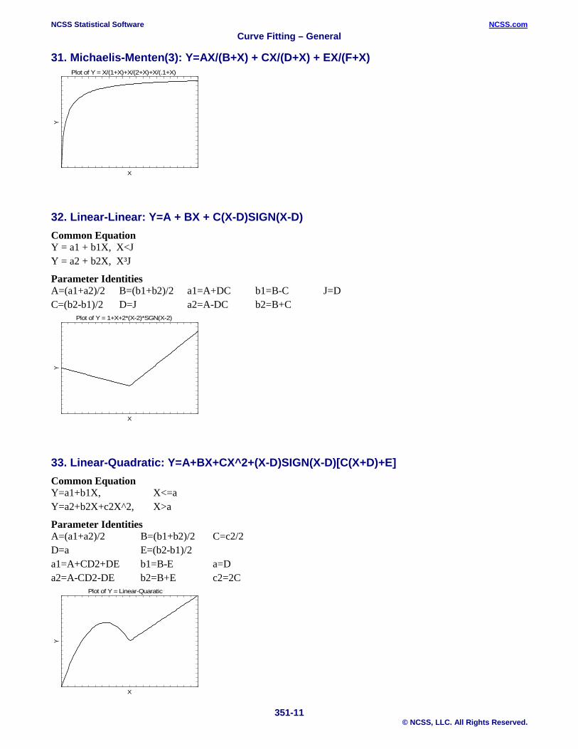
31. Michaelis-Menten(3): Y=AX/(B+X) + CX/(D+X) + EX/(F+X)

32. Linear-Linear: Y=A + BX + C(X-D)SIGN(X-D) Common Equation Y = a1 + b1X, X<J Y = a2 + b2X, X³J

Parameter Identities A=(a1+a2)/2 B=(b1+b2)/2 a1=A+DC b1=B-C J=D C=(b2-b1)/2 D=J a2=A-DC b2=B+C

33. Linear-Quadratic: Y=A+BX+CX^2+(X-D)SIGN(X-D)[C(X+D)+E] Common Equation Y=a1+b1X, X<=a Y=a2+b2X+c2X^2, X>a

Parameter Identities A=(a1+a2)/2 B=(b1+b2)/2 C=c2/2 D=a E=(b2-b1)/2 a1=A+CD2+DE b1=B-E a=D a2=A-CD2-DE b2=B+E c2=2C

Plot of Y = X/(1+X)+X/(2+X)+X/(.1+X)

X

Y

Plot of Y = 1+X+2*(X-2)*SGN(X-2)

X

Y

Plot of Y = Linear-Quaratic

X

Y




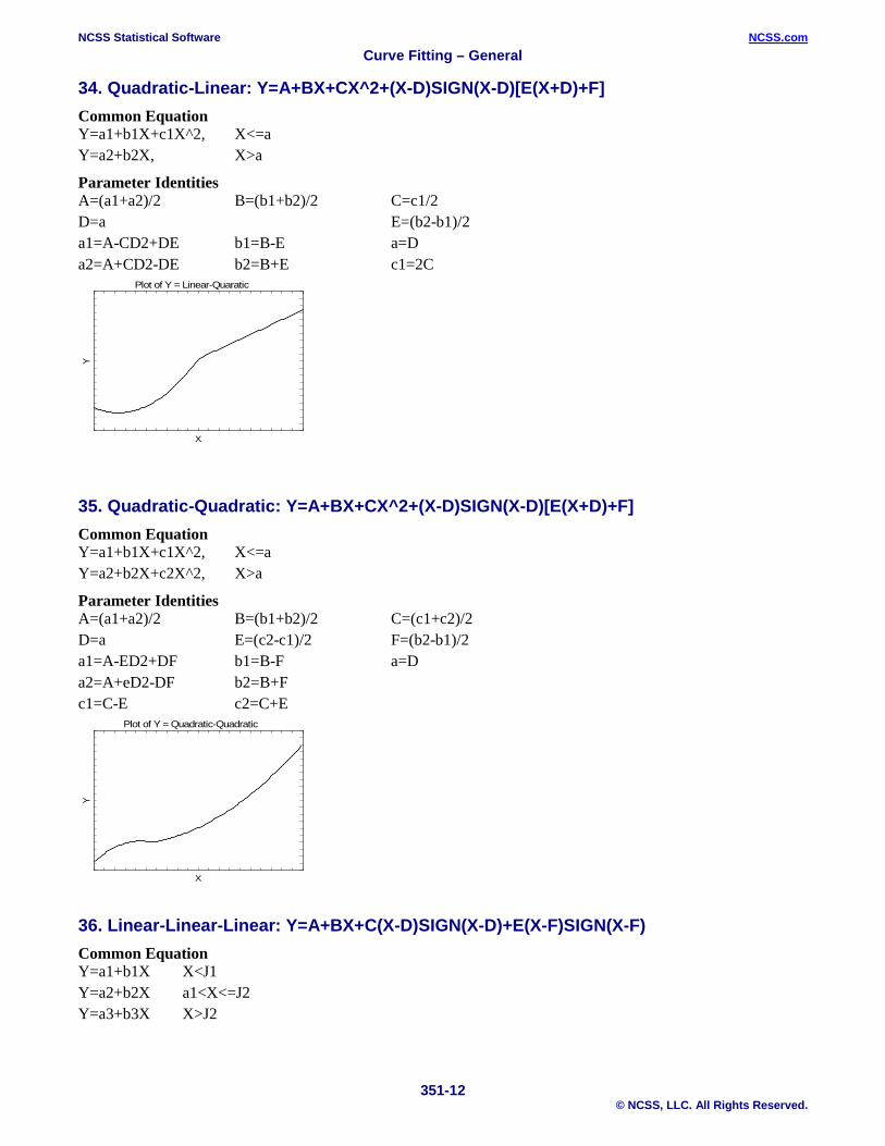
34. Quadratic-Linear: Y=A+BX+CX^2+(X-D)SIGN(X-D)[E(X+D)+F] Common Equation Y=a1+b1X+c1X^2, X<=a Y=a2+b2X, X>a

Parameter Identities A=(a1+a2)/2 B=(b1+b2)/2 C=c1/2 D=a E=(b2-b1)/2 a1=A-CD2+DE b1=B-E a=D a2=A+CD2-DE b2=B+E c1=2C

35. Quadratic-Quadratic: Y=A+BX+CX^2+(X-D)SIGN(X-D)[E(X+D)+F] Common Equation Y=a1+b1X+c1X^2, X<=a Y=a2+b2X+c2X^2, X>a

Parameter Identities A=(a1+a2)/2 B=(b1+b2)/2 C=(c1+c2)/2 D=a E=(c2-c1)/2 F=(b2-b1)/2 a1=A-ED2+DF b1=B-F a=D a2=A+eD2-DF b2=B+F c1=C-E c2=C+E

36. Linear-Linear-Linear: Y=A+BX+C(X-D)SIGN(X-D)+E(X-F)SIGN(X-F) Common Equation Y=a1+b1X X<J1 Y=a2+b2X a1<X<=J2 Y=a3+b3X X>J2

Plot of Y = Linear-Quaratic

X

Y

Plot of Y = Quadratic-Quadratic

X

Y




Parameter Identities A=(a1+a3)/2 B=(b1+b3)/2 C=(b2-b1)/2 D=J1 E=(b3-b2)/2 F=J2 a1=A+CD+EF b1=B-C-E J1=D a2=A-CD-EF b2=B+C-E J2=F a3=A-CD+EF b3=B+C+E

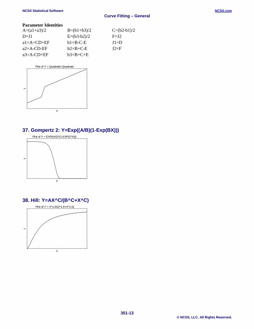
37. Gompertz 2: Y=Exp((A/B)(1-Exp(BX)))

38. Hill: Y=AX^C/(B^C+X^C)

Plot of Y = Quadratic-Quadratic

X

Y

Plot of Y = EXP((4/2)*(1-EXP(2*X)))

X

Y

Plot of Y = X^1.5/(2^1.5+X^1.5)

X

Y




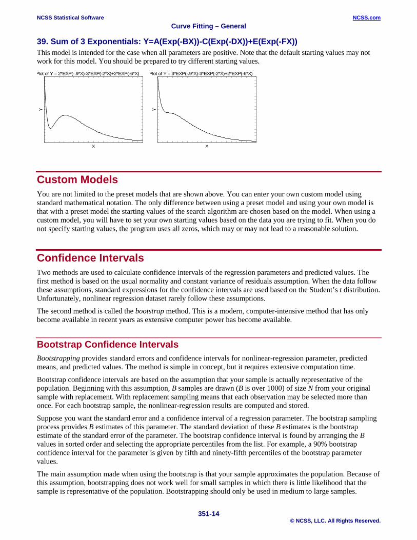
39. Sum of 3 Exponentials: Y=A(Exp(-BX))-C(Exp(-DX))+E(Exp(-FX)) This model is intended for the case when all parameters are positive. Note that the default starting values may not work for this model. You should be prepared to try different starting values.

Custom Models You are not limited to the preset models that are shown above. You can enter your own custom model using standard mathematical notation. The only difference between using a preset model and using your own model is that with a preset model the starting values of the search algorithm are chosen based on the model. When using a custom model, you will have to set your own starting values based on the data you are trying to fit. When you do not specify starting values, the program uses all zeros, which may or may not lead to a reasonable solution.

Confidence Intervals Two methods are used to calculate confidence intervals of the regression parameters and predicted values. The first method is based on the usual normality and constant variance of residuals assumption. When the data follow these assumptions, standard expressions for the confidence intervals are used based on the Student’s t distribution. Unfortunately, nonlinear regression dataset rarely follow these assumptions.

The second method is called the bootstrap method. This is a modern, computer-intensive method that has only become available in recent years as extensive computer power has become available.

Bootstrap Confidence Intervals Bootstrapping provides standard errors and confidence intervals for nonlinear-regression parameter, predicted means, and predicted values. The method is simple in concept, but it requires extensive computation time.

Bootstrap confidence intervals are based on the assumption that your sample is actually representative of the population. Beginning with this assumption, B samples are drawn (B is over 1000) of size N from your original sample with replacement. With replacement sampling means that each observation may be selected more than once. For each bootstrap sample, the nonlinear-regression results are computed and stored.

Suppose you want the standard error and a confidence interval of a regression parameter. The bootstrap sampling process provides B estimates of this parameter. The standard deviation of these B estimates is the bootstrap estimate of the standard error of the parameter. The bootstrap confidence interval is found by arranging the B values in sorted order and selecting the appropriate percentiles from the list. For example, a 90% bootstrap confidence interval for the parameter is given by fifth and ninety-fifth percentiles of the bootstrap parameter values.

The main assumption made when using the bootstrap is that your sample approximates the population. Because of this assumption, bootstrapping does not work well for small samples in which there is little likelihood that the sample is representative of the population. Bootstrapping should only be used in medium to large samples.

Plot of Y = 2*EXP(-.9*X)-3*EXP(-2*X)+2*EXP(-6*X)

X

Y

Plot of Y = 3*EXP(-.9*X)-3*EXP(-2*X)+2*EXP(-6*X)

X

Y




Bootstrap Prediction Intervals Bootstrap confidence intervals for the mean of Y given X are generated from the bootstrap sample in the usual way. To calculate prediction intervals for the predicted value (not the mean) of Y given X requires a modification to the predicted value of Y to be made to account for the variation of Y about its mean. This modification of the predicted Y values in the bootstrap sample, suggested by Davison and Hinkley, is as follows.

*y y e i i r= +

where e r* is a randomly selected modified residual (see below). By adding the residual we have added an

appropriate amount of variation to represent the variance of individual Y’s about their mean value.

Modified Residuals Davison and Hinkley (1999) page 279 recommend the use of a special rescaling of the residuals when bootstrapping to keep results unbiased. Because of the high amount of computing involved in bootstrapping, these modified residuals are calculated using

e e

N

ejj* =−

−1 1

where

ee

N

jj

N

= =∑

1

Note that there is a different rescaling than Davison and Hinkley recommended. We have used this rescaling because it is much quicker to calculate.

Hypothesis Testing When curves are fit to two or more groups, it is often of interest to test whether certain regression parameters are equal and whether the fitted curves coincide. Although some approximate results have been obtained using indicator variables, these are asymptotic results and little is known about their appropriateness in sample samples. We provide a test of the hypothesis that all group curves coincide using an F-test that compares the residual sum of squares obtained when the grouping is

ignored with the total of the residual sum of squares obtained for each group. This test is routinely used in the analysis of variance associated with linear models and its application to nonlinear models has occasionally been suggested. However, it is based on naive assumptions that seldom occur.

Because of the availability of fast computing speed in recent years, a second method of hypothesis testing, called the randomization test, is now available. This test will be discussed next.

Randomization Test Randomization testing is discussed by Edgington (1987). The details of the randomization test are simple: all possible permutations of the group variable while leaving the dependent and independent variables in their original order are investigated. For each permutation, the difference between the estimated group parameters is calculated. The number of permutations with a magnitude greater than or equal to that of the actual sample is counted. Dividing this count by the number of permutations gives the significance level of the test.




The randomization test is suggested because an exact test is achieved without making unrealistic assumptions about the data such as constant variance, normality, or model accuracy. The test was not used in the past because the amount of computations was prohibitive. In fact, the randomization test was originally proposed by Fisher and he chose his F-test because its distribution close approximated the randomization distribution.

The only assumption that a randomization test makes is that the data values are exchangeable under the null hypothesis.

For even moderate sample sizes, the total number of permutations is in the trillions, so a Monte Carlo approach is used in which the permutations are found by random selection rather than enumeration. Using this approach, a reasonable approximation to the test’s probability level may be found by considering only a few thousand permutations rather than the trillions needed for complete enumeration. Edgington suggests that at least 1000 permutations be computed. We suggest that this be increased to 10000 for important results.

The program tests two types of hypotheses using randomization tests. The first is that each of the estimated model parameters is equal. The second is that the individual fitted curves coincide across all groups.

Randomization Statistics for Testing Parameter Equivalence The test statistic for comparing a model parameter is formed by summing the difference between the group parameter estimates for each pair of groups. If there are G groups, the test statistic is computed using the formula

BRT i jj i

G

i

G

= −= +=

−

∑∑ β β11

1

Randomization Statistics for Testing Curve Equivalence The test statistic for comparing the whole curve is formed by summing the difference between the estimated predicted values for each pair of groups at several points along the curve. If there are G groups and K equally spaced test points, the test statistic is computed using the formula

C y yRT ki kjj i

G

i

G

k

K

= −= +=

−

=∑∑∑

11

1

1

Data Structure The data are entered in two variables: one dependent variable and one independent variable. Additionally, you may specify a frequency variable containing the observation count for each row and a group variable that is used to partition the data in to independent groups.

Missing Values Rows with missing values in the variables being analyzed are ignored in the calculations. When only the value of the dependent variable is missing, predicted values are generated.




Procedure Options This section describes the options available in this procedure.

Variables Tab This panel specifies the variables used in the analysis.

Variables

Y (Dependent) Variable Specifies a single dependent (Y) variable from the current dataset. This variable is being predicted using the (preset or custom) model you specify. The actual values fed into the algorithm depend on which transformation (if any) is selected for this variable.

Y Transformation Specifies a power transformation of the dependent variable. Available transformations are

Y’=1/(Y*Y), Y’=1/Y, Y’=1/SQRT(Y), Y’=LN(Y), Y’=SQRT(Y), Y’=Y (none), and Y’=Y*Y

Care must be taken so that you do not apply a transformation that omits much of your data. For example, you cannot take the square root of a negative number, so if you apply this transformation to negative values, those observations will be treated as missing values and ignored. Similarly, you cannot have a zero in the denominator of a quotient and you cannot take the logarithm of a number less than or equal to zero.

X (Independent) Variable Specify the independent (X) variable. This variable is used to predict the dependent variable using the model you have specified. This variable is referred to as ‘X’ in the Preset and Custom model statements. The actual values used depend on which transformation (if any) is selected for this variable.

X Transformation Specifies a power transformation of the independent variable. Available transformations are

X’=1/(X*X), X’=1/X, X’=1/SQRT(X), X’=LN(X), X’=SQRT(X), X’=X (none), and X’=X*X

Care must be taken so that you do not apply a transformation that omits much of your data. For example, you cannot take the square root of a negative number, so if you apply this transformation to negative values, those observations will be treated as missing values and ignored. Similarly, you cannot have a zero in the denominator of a quotient and you cannot take the logarithm of a number less than or equal to zero.

Frequency Variable An optional column containing a set of counts (frequencies). Normally, each row represents one observation. On occasion, however, each row of data may represent more than one observation. This variable contains the number of observations that a row represents. Rows with zeroes and negative values are ignored.

Group Variable This optional variable divides the observations into groups. When specified, a separate analysis is generated for each unique value of this variable. Use the Value Label option under the Format tab to specify the way in which the group values are displayed.




Model

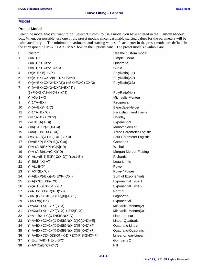
Preset Model Select the model that you want to fit. Select ‘Custom’ to use a model you have entered in the ‘Custom Model’ box. Whenever possible, use one of the preset models since reasonable starting values for the parameters will be calculated for you. The minimum, maximum, and starting values of each letter in the preset model are defined in the corresponding MIN START MAX box on the Options panel. The preset models available are 0 Custom Use the custom model 1 Y=A+BX Simple Linear 2 Y=A+BX+CX^2 Quadratic 3 Y=A+BX+CX^2+DX^3 Cubic 4 Y=(A+BX)/(1+CX) PolyRatio(1,1) 5 Y=(A+BX+CX^2)/(1+DX+EX^2) PolyRatio(2,2) 6 Y=(A+BX+CX^2+DX^3)/(1+EX+FX^2+GX^3) PolyRatio(3,3) 7 Y=(A+BX+CX^2+DX^3+EX^4) / (1+FX+GX^2+HX^3+IX^4) PolyRatio(4,4) 8 Y=AX/(B+X) Michaelis-Menten 9 Y=1/(A+BX) Reciprocal 10 Y=(A+BX)^(-1/C) Bleasdale-Nelder 11 Y=1/(A+BX^C) Farazdaghi and Harris 12 Y=1/(A+BX+CX^2) Holliday 13 Y=EXP(A(X-B)) Exponential 14 Y=A(1-EXP(-B(X-C))) Monomolecular 15 Y=A/(1+B(EXP(-CX))) Three Parameter Logistic 16 Y=D+(A-D)/(1+B(EXP(-CX))) Four Parameter Logistic 17 Y=A(EXP(-EXP(-B(X-C)))) Gompertz 18 Y=A-(A-B)EXP(-(C|X|)^D) Weibull 19 Y=A-(A-B)/(1+(C|X|)^D) Morgan-Mercer-Floding 20 Y=A(1+(B-1)EXP(-C(X-D)))^(1/(1-B)) Richards 21 Y=B(LN(|X|-A)) Logarithmic 22 Y=A(1-B^X) Power 23 Y=AX^(BX^C) Power^Power 24 Y=A(EXP(-BX))+C(EXP(-DX)) Sum of Exponentials 25 Y=A(X^B)EXP(-CX) Exponential Type 1 26 Y=(A+BX)EXP(-CX)+D Exponential Type 2 27 Y=A+B(EXP(-C(X-D)^2)) Normal 28 Y=A+(B/X)EXP(-C(LN(|X|)-D)^2) Lognormal 29 Y=A Exp(-BX) Exponential 30 Y=AX/(B+X) + CX/(D+X) Michaelis-Menten(2) 31 Y=AX/(B+X) + CX/(D+X) + EX/(F+X) Michaelis-Menten(3) 32 Y=A + BX + C(X-D)SIGN(X-D) Linear-Linear 33 Y=A+BX+CX^2+(X-D)SIGN(X-D)[C(X+D)+E] Linear-Quadratic 34 Y=A+BX+CX^2+(X-D)SIGN(X-D)[E(X+D)+F] Quadratic-Linear 35 Y=A+BX+CX^2+(X-D)SIGN(X-D)[E(X+D)+F] Quadratic-Quadratic 36 Y=A+BX+C(X-D)SIGN(X-D)+E(X-F)SIGN(X-F) Linear-Linear-Linear 37 Y=Exp((A/B)(1-Exp(BX))) Gompertz 2 38 Y=AX^C/(B^C+X^C) Hill




Custom Model This box is only used when the Preset Model option is set to ‘Custom Model’. When used, it contains the regression model written in standard mathematical notation.

Use ‘X’ to represent the independent variable specified in the X Variable box, not its variable name. Hence, if your independent variable is HEAT, you would enter A+B*LN(X), not A+B*LN(HEAT).

Use the letters (case ignored) A,B,C,... (except X and Y) to represent the parameters to be estimated from the data. The letters used must be specified in one of the Parameter boxes listed under the Search tab. Note that you do not include a ‘Y=’ in the expression. That is, you would enter A+B*X, not Y=A+B*X.

Expression Syntax Construct the expression using standard mathematical syntax. Possible symbols and functions are

Symbols + add - subtract * multiply / divide ^ exponent (X^2 = X*X) () parentheses < less than. > greater than = equals <= less than or equal >= greater than or equal <> not equal Functions (a logic b) Indicator function. If true, result is 1; otherwise, result is 0. Logic values are <, >, =,

<>, <=, and >=. The symbols a and b are replaced by numbers or letters. ABS(X) Absolute value of X. ARCOSH(X) Arc cosh of X. ARSINH(X) Arc sinh of X. ARTANH(X) Arc tanh of X. ASN(X) Arc sine of X. ATN (X) Arc tangent of X. COS(X) Cosine of X. COSH(X) Hyperbolic cosine of X. ERF(X) The error function of X EXP(X) Exponential of X. INT(X) Integer part of X. LN(X) Log base e of X. LOG(X) Log base 10 of X. LOGGAMMA(X) Log of the gamma function. NORMDENS(X) Normal density. NORMPROB(X) Normal CDF (probability). NORMVALUE(X) Inverse normal CDF. SGN(X) Sign of X which is -1 if X<0, 0 if X=0, and 1 if X>0. SIN(X) Sine of X. SINH(X) Hyperbolic sine of X. SQR(X) Square root of X.




TAN(X) Tangent of X. TANH(X) Hyperbolic tangent of X. TNH(X) Hyperbolic tangent of X. TRIGAMMA(X) Trigamma function.

Independent Variable Use ‘X’ in your expression to represent the independent variable you have specified.

Parameters The letters of the alphabet (except X and Y) may be used to represent the parameters. Parameters can be only one character long and case is ignored. Each parameter must be defined in the Parameter fields below.

Numbers You can enter numbers in standard format such as 23.456 and 254.43, or you can use scientific notation such as 1E-5 (which is 0.00001) and 1E5 (which is 100000).

Examples Standard mathematical syntax is used. This is discussed in detail in the Transformation section. Examples of valid expressions are: A+B*X

C+D*X+E*X*X or G+H*X+B*X^2

A*EXP(B*X)

(X<=5)*A+(X>5)*B+C

Bias Correction This option controls whether a bias-correction factor is applied when the dependent variable has been transformed. Check it to correct the predicted values for the transformation bias. Uncheck it to leave the predicted values unchanged. See the Introduction to Curve Fitting chapter for a discussion of the amount of bias that may occur and the bias correction procedures used.

Model Parameters The following options control the nonlinear regression algorithm.

Parameter Enter a letter (other than X and Y) used in the Model. Note that the case of the character is ignored. Each letter used in a Model (either Preset or Custom) must be defined in this section by entering its letter, bounds, and starting value.

For example, suppose the model is A + B*X + C*X^2. The parameters in this expression are A, B, and C. Each must be defined here.

Min Start Max Enter the minimum, starting value, and maximum of this parameter by entering three numbers separated by blanks or commas. You may enter ‘?’ as the starting value to instruct the program pick one for you (in which case a zero is often used). The program searches for the best value between the minimum and the maximum values, beginning with the starting value.

Make sure that the starting values you supply are possible. For example, if the model includes the phrase 1/B, don’t start with B=0. Before taking a lot of time trying to find a starting value, make a few trial runs using starting values of 0.0, 0.1, and 1.0. Often, one of these values will work.




Examples -1000 1 1000 which means starting value = 1, lower bound = -1000, and upper bound = 1000.

-1 ? 1E9 which means starting value is unspecified, lower bound = -1, and upper bound = 1000000000.

• Minimum This is the smallest value that the parameter can take on. The algorithm searches for a value between this and the maximum. If you want to search in an unlimited range, enter a large negative number such as -1E9, which is -1000000000.

Since this is a search algorithm, the narrower the range that you search in, the quicker it will converge.

Care should be taken to specify minima and maxima that keep calculations in range. Suppose, for example, that your equation includes the expression LOG(B*X) and that values of X are positive. Since you cannot take the logarithm of zero or a negative number, you should set the minimum of B as a small positive number, insuring that the estimation procedure will not fail because of impossible calculations.

• Starting Value Enter a starting value for this parameter or enter ‘?’ to have the system estimate a starting value for you. When using a custom model, a ‘?’ is replaced by zero.

• Maximum This is the largest value that the parameter can take on. The algorithm searches for a value between the minimum and this value, beginning at the Starting Value. If you want to search in an unlimited range, enter a large positive number such as 1E9, which is 1000000000.

Since this is a search algorithm, the narrower the range that you search in, the quicker the process will converge.

Resampling

Bootstrap Confidence Intervals This option causes bootstrap confidence intervals and associated bootstrap reports and plots to be generated using resampling simulation as specified under the Resampling tab.

Bootstrapping may be time consuming when the bootstrap sample size is large. A reasonable strategy is to keep this option unchecked until you have considered all other reports. Then run this option with a bootstrap size of 100 or 1000 to obtain an idea of the time needed to complete the simulation.

Randomization Hypothesis Tests This option hypothesis tests and associated reports to be generated using Monte Carlo simulation as specified under the Resampling tab.

Randomization tests may be time consuming when the Monte Carlo sample size is large. A reasonable strategy is to keep this option unchecked until you have run and considered all other reports. Then run this option with a Monte Carlo size of 100, then 1000, and then 10000 to obtain an idea of the time needed to complete the simulation.




Options Tab The following options control the nonlinear regression algorithm.

Options

Lambda This is the starting value of the lambda parameter as defined in Marquardt’s procedure. We recommend that you do not change this value unless you are very familiar with both your model and the Marquardt nonlinear regression procedure. Changing this value will influence the speed at which the algorithm converges.

Nash Phi Nash supplies a factor he calls phi for modifying lambda. When the residual sum of squares is large, increasing this value may speed convergence.

Lambda Inc This is a factor used for increasing lambda when necessary. It influences the rate at which the algorithm converges.

Lambda Dec This is a factor used for decreasing lambda when necessary. It also influences the rate at which the algorithm converges.

Max Iterations This sets the maximum number of iterations before the program aborts. If the starting values you have supplied are not appropriate or the model does not fit the data, the algorithm may diverge. Setting this value to an appropriate number (say 50) causes the algorithm to abort after this many iterations.

Zero This is the value used as zero by the nonlinear algorithm. Because of rounding error, values lower than this value are reset to zero. If unexpected results are obtained, you might try using a smaller value, such as 1E-16. Note that 1E-5 is an abbreviation for the number 0.00001.

Reports Tab This section controls which reports and plots are displayed.

Select Reports

Combined Summary Report ... Residual Report These options specify which reports are displayed.

Predicted Values

Predict Y at these X Values Enter an optional list of X values at which to report the predicted value of Y and corresponding confidence interval. You can enter a single number or a list of numbers. The list can be separated with commas or spaces. The list can also be of the form ‘XX:YY(ZZ)’ which means XX to YY by ZZ.




Examples 10

10 20 30 40 50

0:90(10) which means 0 10 20 30 40 50 60 70 80 90

100:950(200) which means 100 300 500 700 900

1000:5000(500) which means 1000 1500 2000 2500 3000 3500 4000 4500 5000

Report Options

Alpha Level Enter the value of alpha for the confidence limits. Usually, this number will range from 0.1 to 0.001. A common choice for alpha is 0.05. You should determine a value appropriate for your needs.

Precision Specify the precision of numbers in the report. Single precision will display seven-place accuracy, while the double precision will display thirteen-place accuracy. Note that all reports are formatted for single precision only.

Variable Names Specify whether to use variable names or (the longer) variable labels in report headings.

Value Labels Value Labels may be used with the Group Variable to make reports more legible by assigning meaningful labels to numbers and codes.

• Data Values All data are displayed in their original format, regardless of whether a value label has been set or not.

• Value Labels All values of variables that have a value label variable designated are converted to their corresponding value label when they are output. This does not modify their value during computation.

• Both Both data value and value label are displayed.

Example A variable named GENDER (used as a grouping variable) contains 1's and 2's. By specifying a value label for GENDER, the printout will display Male instead of 1 and Female instead of 2 on the reports. This option specifies whether (and how) to use the value labels.




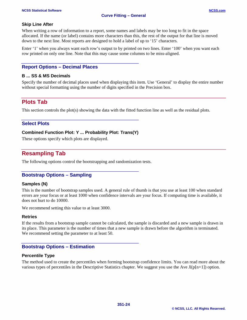
Skip Line After When writing a row of information to a report, some names and labels may be too long to fit in the space allocated. If the name (or label) contains more characters than this, the rest of the output for that line is moved down to the next line. Most reports are designed to hold a label of up to ‘15’ characters.

Enter ‘1’ when you always want each row’s output to by printed on two lines. Enter ‘100’ when you want each row printed on only one line. Note that this may cause some columns to be miss-aligned.

Report Options – Decimal Places

B ... SS & MS Decimals Specify the number of decimal places used when displaying this item. Use ‘General’ to display the entire number without special formatting using the number of digits specified in the Precision box.

Plots Tab This section controls the plot(s) showing the data with the fitted function line as well as the residual plots.

Select Plots

Combined Function Plot: Y ... Probability Plot: Trans(Y) These options specify which plots are displayed.

Resampling Tab The following options control the bootstrapping and randomization tests.

Bootstrap Options – Sampling

Samples (N) This is the number of bootstrap samples used. A general rule of thumb is that you use at least 100 when standard errors are your focus or at least 1000 when confidence intervals are your focus. If computing time is available, it does not hurt to do 10000.

We recommend setting this value to at least 3000.

Retries If the results from a bootstrap sample cannot be calculated, the sample is discarded and a new sample is drawn in its place. This parameter is the number of times that a new sample is drawn before the algorithm is terminated. We recommend setting the parameter to at least 50.

Bootstrap Options – Estimation

Percentile Type The method used to create the percentiles when forming bootstrap confidence limits. You can read more about the various types of percentiles in the Descriptive Statistics chapter. We suggest you use the Ave X(p[n+1]) option.




C.I. Method This option specifies the method used to calculate the bootstrap confidence intervals. The reflection method is recommended.

• Percentile The confidence limits are the corresponding percentiles of the bootstrap values.

• Reflection The confidence limits are formed by reflecting the percentile limits. If X0 is the original value of the parameter estimate and XL and XU are the percentile confidence limits, the Reflection interval is (2 X0 - XU, 2 X0 - XL).

Bootstrap Confidence Coefficients These are the confidence coefficients of the bootstrap confidence intervals. Since bootstrapping calculations may take several minutes, it may be useful to obtain confidence intervals using several different confidence coefficients.

All values must be between 0.50 and 1.00. You may enter several values, separated by blanks or commas. A separate confidence interval is given for each value entered.

Examples 0.90 0.95 0.99

0.90:0.99(0.01)

0.90

Randomization Test Options

Monte Carlo Samples Specify the number of Monte Carlo samples used when running randomization tests. Somewhere between 1000 and 100000 are usually necessary. Although we use 1000 as the default value, a better value for routine use is 10000.

You also need to check the ‘Randomization Hypothesis Tests’ box on the Variables tab to run these tests.

Comparative Points Specify the number of X values at which the difference between group curves is computed. This is the value of K in the formula given earlier. The sum of the absolute values of these differences is use in the randomization test of whether the group curves coincide.

Random Number Seed

Random Number Seed This option specifies a random seed for the random number generator. Possible values are all integers between 1 and 32000. If you want to obtain the same results from one run to the next, use the same seed value. If you want to let the program select a random seed based on the time-of-day, enter ‘RANDOM SEED’.

Storage Tab The predicted values and residuals may be stored on the current database for further analysis. This group of options lets you designate which statistics (if any) should be stored and which variables should receive these statistics. The selected statistics are automatically stored to the current database while the program is executing.




Note that existing data is replaced. Be careful that you do not specify variables that contain important data.

Storage Variables

Store Predicted Values, Residuals, Lower Prediction Limit, and Upper Prediction Limit The predicted (Yhat) values, residuals (Y-Yhat), lower 100(1-alpha) prediction limits, and upper 100(1-alpha) prediction limits may be stored in the columns specified here.

Example 1 – Curve Fitting This section presents an example of how to fit and compare a Michaelis-Menten model (model 8) to two groups of data. This example will use the data in the FnReg5 dataset. In this example, the dependent variable is Response and the independent variable is Temp. The groups are defined by the values of Type.

You may follow along here by making the appropriate entries or load the completed template Example 1 by clicking on Open Example Template from the File menu of the Curve Fitting – General window.

1 Open the FnReg5 dataset. • From the File menu of the NCSS Data window, select Open Example Data. • Click on the file FnReg5.NCSS. • Click Open.

2 Open the Curve Fitting – General window. • Using the Analysis menu or the Procedure Navigator, find and select the Curve Fitting – General

procedure. • On the menus, select File, then New Template. This will fill the procedure with the default template.

3 Specify the variables. • Select the Variables tab. • Set the Y Variable to Response. • Set the X Variable to Temp. • Set the Group Variable to Type. • Set the Preset Model to 8 Y=AX/(B+X) Michaelis-Menten. • Check the Bootstrap Confidence Intervals box. • Check the Randomization Hypothesis Tests box.

4 Specify the reports. • Select the Reports tab. • Check all reports and plots except the Iteration Detail Report. • Set the Predict Y at these X Values to 5 10 15 20.

5 Specify the resampling. • Select the Resampling tab. • Set Samples (N) to 200. (We are using a small value for illustrative purposes. You should use at least

3000 when actually using the results.) • Set Monte Carlo Samples to 200. (We are using a small value for illustrative purposes. You should use

at least 1000 when actually using the results.) • Set Random Number Seed to 17448. (Use this number so that our reports agree. Usually you would

leave this set to ‘RANDOM START’.)




6 Run the procedure. • From the Run menu, select Run Procedure. Alternatively, just click the green Run button.

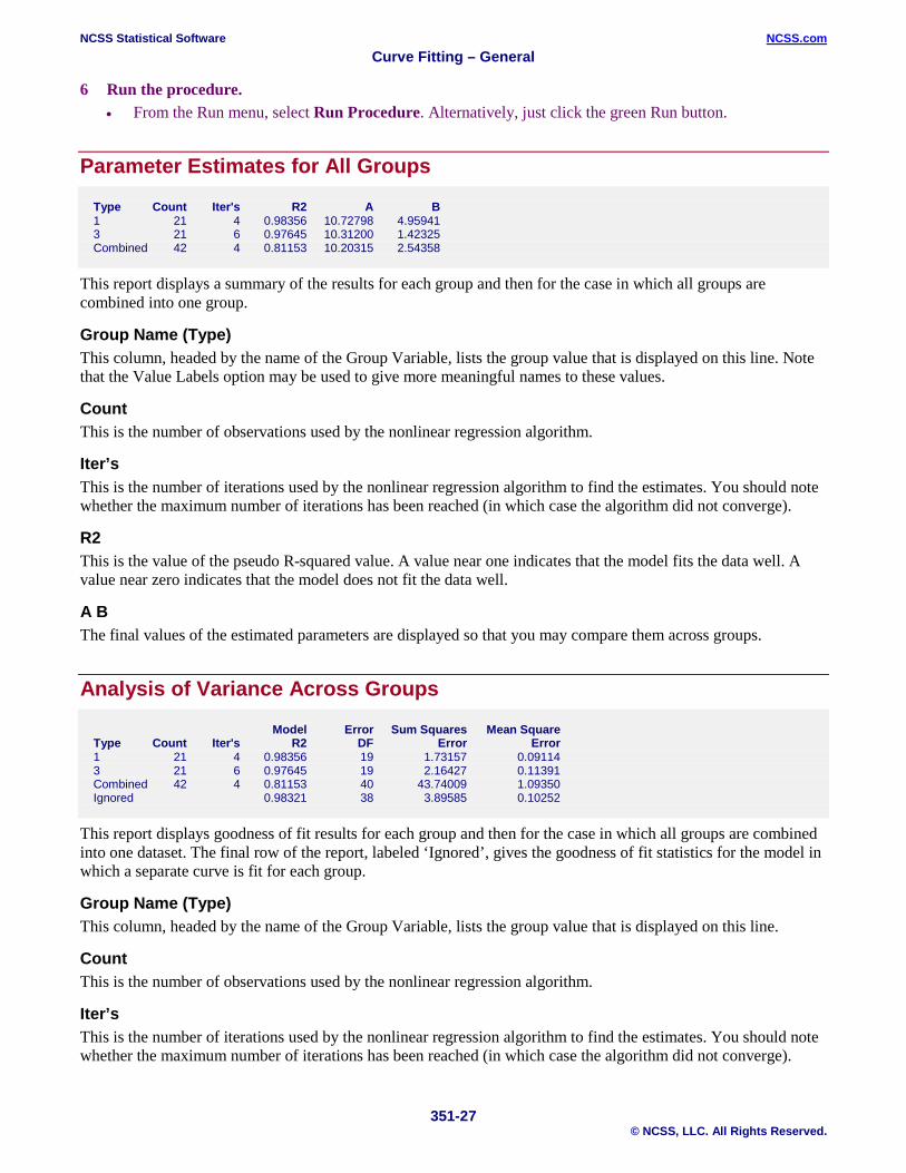
Parameter Estimates for All Groups

Type Count Iter's R2 A B 1 21 4 0.98356 10.72798 4.95941 3 21 6 0.97645 10.31200 1.42325 Combined 42 4 0.81153 10.20315 2.54358

This report displays a summary of the results for each group and then for the case in which all groups are combined into one group.

Group Name (Type) This column, headed by the name of the Group Variable, lists the group value that is displayed on this line. Note that the Value Labels option may be used to give more meaningful names to these values.

Count This is the number of observations used by the nonlinear regression algorithm.

Iter’s This is the number of iterations used by the nonlinear regression algorithm to find the estimates. You should note whether the maximum number of iterations has been reached (in which case the algorithm did not converge).

R2 This is the value of the pseudo R-squared value. A value near one indicates that the model fits the data well. A value near zero indicates that the model does not fit the data well.

A B The final values of the estimated parameters are displayed so that you may compare them across groups.

Analysis of Variance Across Groups

Model Error Sum Squares Mean Square Type Count Iter's R2 DF Error Error 1 21 4 0.98356 19 1.73157 0.09114 3 21 6 0.97645 19 2.16427 0.11391 Combined 42 4 0.81153 40 43.74009 1.09350 Ignored 0.98321 38 3.89585 0.10252

This report displays goodness of fit results for each group and then for the case in which all groups are combined into one dataset. The final row of the report, labeled ‘Ignored’, gives the goodness of fit statistics for the model in which a separate curve is fit for each group.

Group Name (Type) This column, headed by the name of the Group Variable, lists the group value that is displayed on this line.

Count This is the number of observations used by the nonlinear regression algorithm.

Iter’s This is the number of iterations used by the nonlinear regression algorithm to find the estimates. You should note whether the maximum number of iterations has been reached (in which case the algorithm did not converge).




R2 This is the value of the pseudo R-squared value. A value near one indicates that the model fits the data well. A value near zero indicates that the model does not fit the data well. Note

Error DF The degrees of freedom are the number of observations minus the number of parameters fit.

Sum Squares Error This is the sum of the squared residuals for this group.

Mean Square Error This is a rough estimate of the variance of the residuals for this group.

Curve Inequality F-Test

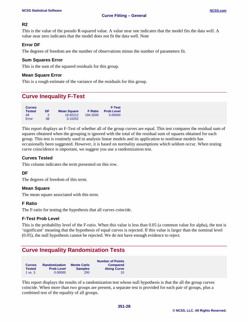
Curves F-Test Tested DF Mean Square F Ratio Prob Level All 2 19.92212 194.3200 0.00000 Error 38 0.10252

This report displays an F-Test of whether all of the group curves are equal. This test compares the residual sum of squares obtained when the grouping is ignored with the total of the residual sum of squares obtained for each group. This test is routinely used in analysis linear models and its application to nonlinear models has occasionally been suggested. However, it is based on normality assumptions which seldom occur. When testing curve coincidence is important, we suggest you use a randomization test.

Curves Tested This column indicates the term presented on this row.

DF The degrees of freedom of this term.

Mean Square The mean square associated with this term.

F Ratio The F-ratio for testing the hypothesis that all curves coincide.

F-Test Prob Level This is the probability level of the F-ratio. When this value is less than 0.05 (a common value for alpha), the test is ‘significant’ meaning that the hypothesis of equal curves is rejected. If this value is larger than the nominal level (0.05), the null hypothesis cannot be rejected. We do not have enough evidence to reject.

Curve Inequality Randomization Tests Number of Points Curves Randomization Monte Carlo Compared Tested Prob Level Samples Along Curve 1 vs. 3 0.00000 200 10

This report displays the results of a randomization test whose null hypothesis is that the all the group curves coincide. When more than two groups are present, a separate test is provided for each pair of groups, plus a combined test of the equality of all groups.




Curves Tested This column indicates the groups whose equality is being test on this row.

Randomization Prob Level This is the two-sided probability level of the randomization test. When this value is less than 0.05, the test is ‘significant’ meaning that the null hypothesis of equal curves is rejected. If this value is larger than the nominal level (0.05), there is not enough evidence in the data to reject the null hypothesis of equality.

(Note: because this is a Monte Carlo test, your results may vary from those displayed here.)

Monte Carlo Samples The number of Monte Carlo samples.

Number of Points Compared Along the Curve The number of values along the X axis at which a comparison between curves is made. Of course, the more X values used, the more accurate (and time consuming) will be the test.

Parameter Inequality Randomization Tests Curves Parameter Randomization Monte Carlo Compared Tested Prob Level Iterations 1 vs. 3 A 0.70000 200 1 vs. 3 B 0.02500 200

This report displays the results of randomization tests about the equality of each parameter across groups. When more than two groups are present, a separate test is provided for each pair of groups, plus a combined test of parameter equality of all groups.

Curves Compared This column indicates the groups being test on this row.

Parameter Test This column indicates model parameter whose equality is being tested.

Randomization Prob Level This is the two-sided probability level of the randomization test. When this value is less than 0.05, the test is ‘significant’ meaning that the null hypothesis of equal parameter values across groups is rejected. If this value is larger than the nominal level (0.05), there is not enough evidence in the data to reject the null hypothesis of equality.

(Note: because this is a Monte Carlo test, your results may vary from those displayed here.)

Monte Carlo Samples The number of Monte Carlo samples.

Number of Points Compared Along the Curve The number of values along the X axis at which a comparison between curves is made. Of course, the more X values used, the more accurate (and time consuming) will be the test.




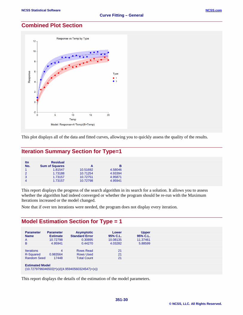
Combined Plot Section

This plot displays all of the data and fitted curves, allowing you to quickly assess the quality of the results.

Iteration Summary Section for Type=1 Itn Residual No. Sum of Squares A B 1 1.81547 10.51692 4.58046 2 1.73188 10.71254 4.93394 3 1.73157 10.72751 4.95871 4 1.73157 10.72798 4.95941

This report displays the progress of the search algorithm in its search for a solution. It allows you to assess whether the algorithm had indeed converged or whether the program should be re-run with the Maximum Iterations increased or the model changed. Note that if over ten iterations were needed, the program does not display every iteration.

Model Estimation Section for Type = 1

Parameter Parameter Asymptotic Lower Upper Name Estimate Standard Error 95% C.L. 95% C.L. A 10.72798 0.30895 10.08135 11.37461 B 4.95941 0.44270 4.03282 5.88599 Iterations 4 Rows Read 21 R-Squared 0.983564 Rows Used 21 Random Seed 17448 Total Count 21 Estimated Model (10.7279796046503)*(x)/((4.95940560324547)+(x))

This report displays the details of the estimation of the model parameters.




Parameter Name The name of the parameter whose results are shown on this line.

Parameter Estimate The estimated value of this parameter.

Asymptotic Standard Error An estimate of the standard error of the parameter based on asymptotic (large sample) results.

Lower 95% C.L. The lower value of a 95% confidence limit for this parameter. This is a large sample (at least 25 observations for each parameter) confidence limit. In most cases, the bootstrap confidence interval will be more accurate.

Upper 95% C.L. The upper value of a 95% confidence limit for this parameter. This is a large sample (at least 25 observations for each parameter) confidence limit. In most cases, the bootstrap confidence interval will be more accurate.

Iterations The number of iterations that were completed before the nonlinear algorithm terminated. If the number of iterations is equal to the Maximum Iterations that you set, the algorithm did not converge, but was aborted.

R-Squared There is no direct R-squared defined for nonlinear regression. This is a pseudo R-squared constructed to approximate the usual R-squared value used in multiple regression. We use the following generalization of the usual R-squared formula:

R-Squared = (ModelSS - MeanSS)/(TotalSS-MeanSS)

where MeanSS is the sum of squares due to the mean, ModelSS is the sum of squares due to the model, and TotalSS is the total (uncorrected) sum of squares of Y (the dependent variable).

This version of R-squared tells you how well the model performs after removing the influence of the mean of Y. Since many nonlinear models do not explicitly include a parameter for the mean of Y, this R-squared may be negative (in which case we set it to zero) or difficult to interpret. However, if you think of it as a direct extension of the R-squared that you use in multiple regression, it will serve well for comparative purposes.

Random Seed This is the value of the random seed that was used when running the bootstrap confidence intervals and randomization tests. If you want to duplicate your results exactly, enter this random seed into the Random Seed box under the Simulation tab.

Estimated Model This is the model that was estimated with the parameters replaced with their estimated values. This expression may be copied and pasted as a variable transformation in the spreadsheet. This will allow you to predict for additional values of X. Note that to insure accuracy, the parameter estimates are always given to double-precision accuracy.




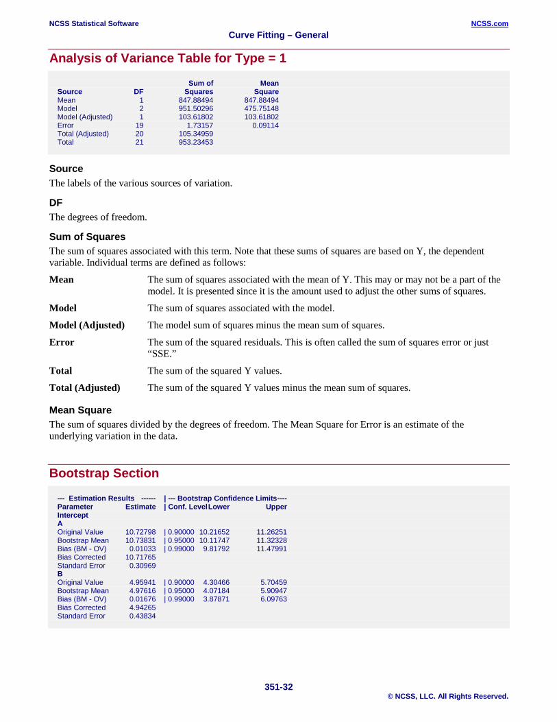
Analysis of Variance Table for Type = 1

Sum of Mean Source DF Squares Square Mean 1 847.88494 847.88494 Model 2 951.50296 475.75148 Model (Adjusted) 1 103.61802 103.61802 Error 19 1.73157 0.09114 Total (Adjusted) 20 105.34959 Total 21 953.23453

Source The labels of the various sources of variation.

DF The degrees of freedom.

Sum of Squares The sum of squares associated with this term. Note that these sums of squares are based on Y, the dependent variable. Individual terms are defined as follows:

Mean The sum of squares associated with the mean of Y. This may or may not be a part of the model. It is presented since it is the amount used to adjust the other sums of squares.

Model The sum of squares associated with the model.

Model (Adjusted) The model sum of squares minus the mean sum of squares.

Error The sum of the squared residuals. This is often called the sum of squares error or just “SSE.”

Total The sum of the squared Y values.

Total (Adjusted) The sum of the squared Y values minus the mean sum of squares.

Mean Square The sum of squares divided by the degrees of freedom. The Mean Square for Error is an estimate of the underlying variation in the data.

Bootstrap Section --- Estimation Results ------ | --- Bootstrap Confidence Limits ---- Parameter Estimate | Conf. Level Lower Upper Intercept A Original Value 10.72798 | 0.90000 10.21652 11.26251 Bootstrap Mean 10.73831 | 0.95000 10.11747 11.32328 Bias (BM - OV) 0.01033 | 0.99000 9.81792 11.47991 Bias Corrected 10.71765 Standard Error 0.30969 B Original Value 4.95941 | 0.90000 4.30466 5.70459 Bootstrap Mean 4.97616 | 0.95000 4.07184 5.90947 Bias (BM - OV) 0.01676 | 0.99000 3.87871 6.09763 Bias Corrected 4.94265 Standard Error 0.43834




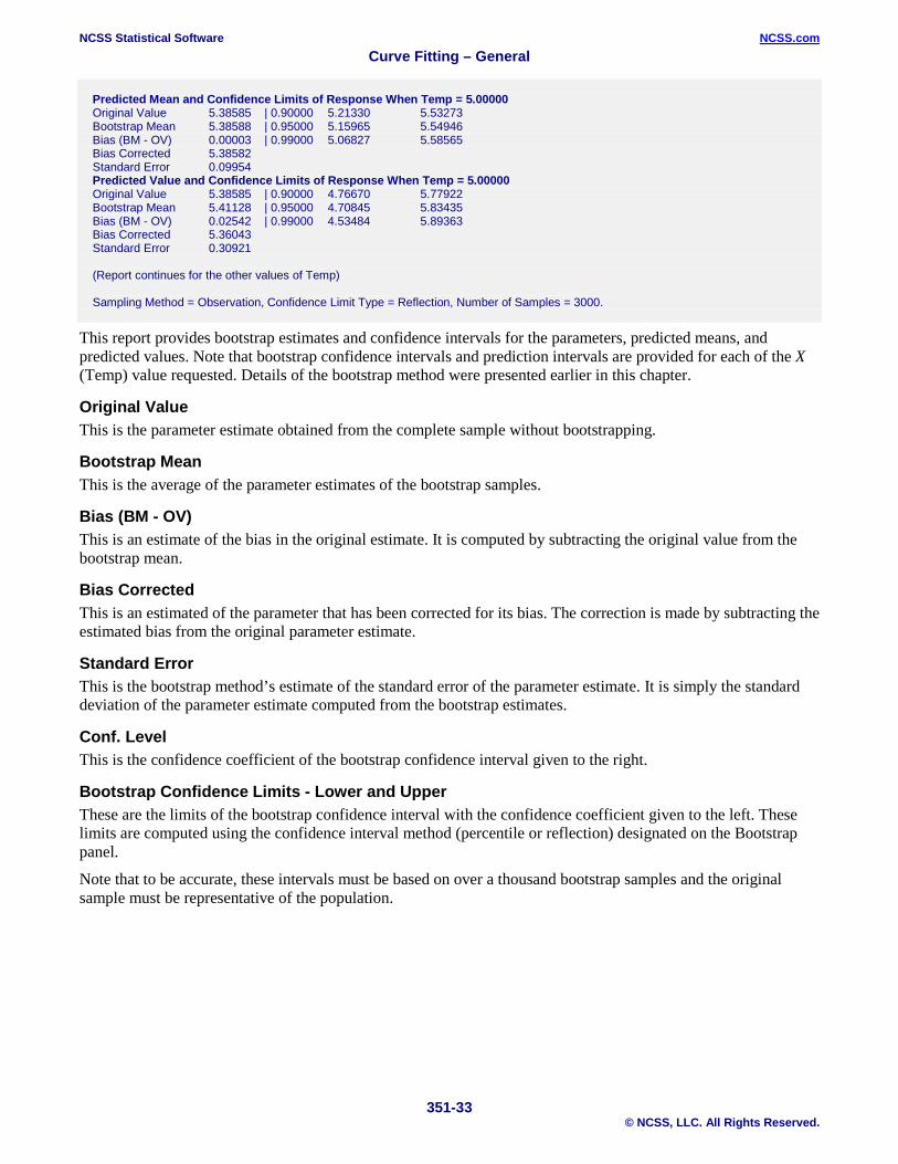
Predicted Mean and Confidence Limits of Response When Temp = 5.00000 Original Value 5.38585 | 0.90000 5.21330 5.53273 Bootstrap Mean 5.38588 | 0.95000 5.15965 5.54946 Bias (BM - OV) 0.00003 | 0.99000 5.06827 5.58565 Bias Corrected 5.38582 Standard Error 0.09954 Predicted Value and Confidence Limits of Response When Temp = 5.00000 Original Value 5.38585 | 0.90000 4.76670 5.77922 Bootstrap Mean 5.41128 | 0.95000 4.70845 5.83435 Bias (BM - OV) 0.02542 | 0.99000 4.53484 5.89363 Bias Corrected 5.36043 Standard Error 0.30921 (Report continues for the other values of Temp) Sampling Method = Observation, Confidence Limit Type = Reflection, Number of Samples = 3000.

This report provides bootstrap estimates and confidence intervals for the parameters, predicted means, and predicted values. Note that bootstrap confidence intervals and prediction intervals are provided for each of the X (Temp) value requested. Details of the bootstrap method were presented earlier in this chapter.

Original Value This is the parameter estimate obtained from the complete sample without bootstrapping.

Bootstrap Mean This is the average of the parameter estimates of the bootstrap samples.

Bias (BM - OV) This is an estimate of the bias in the original estimate. It is computed by subtracting the original value from the bootstrap mean.

Bias Corrected This is an estimated of the parameter that has been corrected for its bias. The correction is made by subtracting the estimated bias from the original parameter estimate.

Standard Error This is the bootstrap method’s estimate of the standard error of the parameter estimate. It is simply the standard deviation of the parameter estimate computed from the bootstrap estimates.

Conf. Level This is the confidence coefficient of the bootstrap confidence interval given to the right.

Bootstrap Confidence Limits - Lower and Upper These are the limits of the bootstrap confidence interval with the confidence coefficient given to the left. These limits are computed using the confidence interval method (percentile or reflection) designated on the Bootstrap panel.

Note that to be accurate, these intervals must be based on over a thousand bootstrap samples and the original sample must be representative of the population.




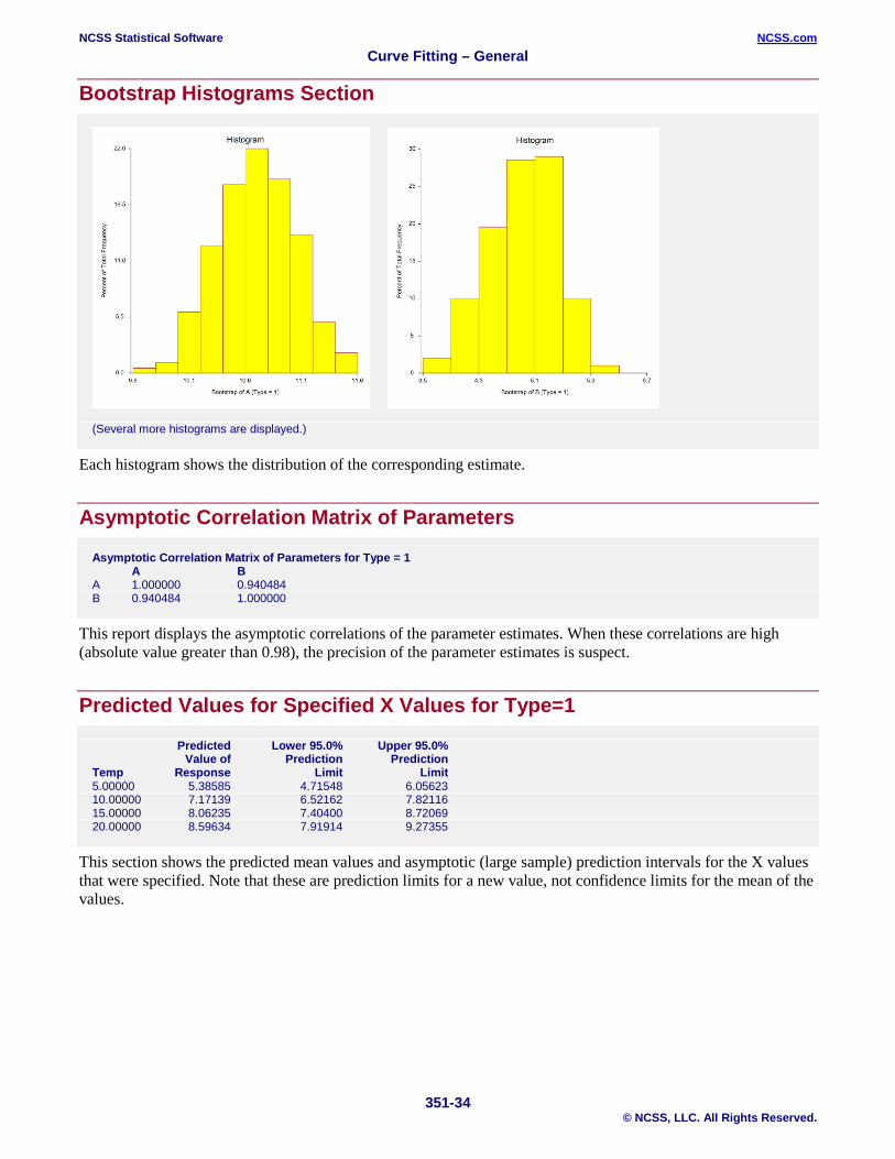
Bootstrap Histograms Section

(Several more histograms are displayed.)

Each histogram shows the distribution of the corresponding estimate.

Asymptotic Correlation Matrix of Parameters

Asymptotic Correlation Matrix of Parameters for Type = 1 A B A 1.000000 0.940484 B 0.940484 1.000000

This report displays the asymptotic correlations of the parameter estimates. When these correlations are high (absolute value greater than 0.98), the precision of the parameter estimates is suspect.

Predicted Values for Specified X Values for Type=1

Predicted Lower 95.0% Upper 95.0% Value of Prediction Prediction Temp Response Limit Limit 5.00000 5.38585 4.71548 6.05623 10.00000 7.17139 6.52162 7.82116 15.00000 8.06235 7.40400 8.72069 20.00000 8.59634 7.91914 9.27355

This section shows the predicted mean values and asymptotic (large sample) prediction intervals for the X values that were specified. Note that these are prediction limits for a new value, not confidence limits for the mean of the values.




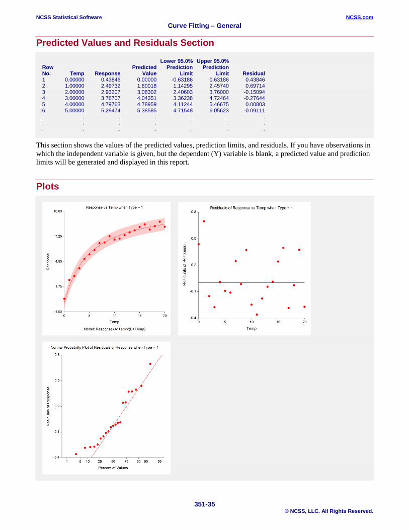
Predicted Values and Residuals Section

Lower 95.0% Upper 95.0% Row Predicted Prediction Prediction No. Temp Response Value Limit Limit Residual 1 0.00000 0.43846 0.00000 -0.63186 0.63186 0.43846 2 1.00000 2.49732 1.80018 1.14295 2.45740 0.69714 3 2.00000 2.93207 3.08302 2.40603 3.76000 -0.15094 4 3.00000 3.76707 4.04351 3.36238 4.72464 -0.27644 5 4.00000 4.79763 4.78959 4.11244 5.46675 0.00803 6 5.00000 5.29474 5.38585 4.71548 6.05623 -0.09111 . . . . . . . . . . . . . . . . . . . . .

This section shows the values of the predicted values, prediction limits, and residuals. If you have observations in which the independent variable is given, but the dependent (Y) variable is blank, a predicted value and prediction limits will be generated and displayed in this report.

Plots




Normal Probability Plot If the residuals are normally distributed, the data points of the normal probability plot will fall along a straight line. Major deviations from this ideal picture reflect departures from normality. Stragglers at either end of the normal probability plot indicate outliers, curvature at both ends of the plot indicates long or short distributional tails, convex or concave curvature indicates a lack of symmetry, and gaps or plateaus or segmentation in the normal probability plot may require a closer examination of the data or model. We do not recommend that you use this diagnostic with small sample sizes.

Residual versus X Plot This is a scatter plot of the residuals versus the independent variable, X. The preferred pattern is a rectangular shape or point cloud. Any nonrandom pattern may require a redefinition of the model.

Function Plot This plot displays the data along with the estimated function. It is useful in deciding if the fit is adequate and the prediction limits are appropriate.


Curve Fitting – General - NCSS · Curve Fitting – General Introduction Curve fitting refers to...

Documents

Transcript of Curve Fitting – General - NCSS · Curve Fitting – General Introduction Curve fitting refers to...