1

CURSO Minería de Datos Predictiva con

SPSS/IBM Modeler Mayo-Junio 2016

Profesor: Ramón Mahía (ramon.mahia@uam.es)

CLUSTER ANALYISIS K-MEANS & TWOSTEP in IBM-MODELER

OBJECTIVES:

1. Understand the basic similarities and differences between Two – Step

cluster and K-Means algorithms

2. Briefly describe K-Means and Two – Step Cluster algorithms mechanisms

3. Basic settings for Two – Step & K-Means nodes in IBM-Modeler

4. Interpretation of Modeler output for Two – Step & K-Means using IBM-

Modeler

2

1.- TWO – STEP and K-MEANS cluster algorithms: similarities and differences

There are many different clustering methods, but in the area of data mining only a few of simpler

methods are widely used, such as K-Means, Two-Step or Kohonen (neural network based). K-Means

and Two-Step algorithms provided by IBM-Modeler are both popular methods for running quick cluster

analysis in an easy to interpret, simple and fast way. On the contrary, the family of so called hierarchical

algorithms are not a good option because of computational cost associated to the massive size of

datasets.

K-Means cluster

Normally, the decision is not about to select K-Means Vs Two-Step given that both algorithms share

some common advantages. K-Means is a very popular non-hierarchical cluster algorithm with some

interesting features:

1. It is easy to implement, even using our own program coding

2. Is a relatively quick method for exploring clusters in data (if we keep “k” small)

3. The procedure find very good cluster solutions when clusters are well-spaced

Some disadvantages, commonly mentioned might be:

1. It is difficult to predict what “K” should be

2. The result may be somehow dependent of initial cluster’s centers (see technical note

below)

Two STEP Cluster

Two STEP Cluster is also a very well - known algorithm is widely used to run cluster exercises because

of some interesting peculiarities. Like K-Means it works for large datasets but, unlike K-Means, it has

some very interesting advantages:

1. When we need to consider BOTH categorical and numerical variables at the same time

Two Step can produce solutions based on mixtures of continuous and categorical

variables. (It has to be said that Modeler also allows the use of categorical variables using

K-Means but they are previously transformed into FLAG variables)

2. Automatic selection of “IDEAL” number of clusters. By automatically comparing the

values of a model-choice criterion across different clustering solutions, the procedure can

automatically determine the “optimal” (technically speaking) number of clusters.

3. Automatic outliers / atypical data handling

As a disadvantage, there is a penalty to the cluster quality for assuming a certain probability

distribution for continuous and categorical variables (which might not be correct) when applying log-

likelihood measurement (see technical note below). This assumption might be wrong, affecting the

quality of cluster solution.

3

2.- A very brief technical note about K-Means and Two – step cluster algorithms

K-Means cluster ALGORITHM

The K-Means algorithm uses a very effective way of recognizing existing groups by applying an iterative

simple procedure:

1. We start by selecting the set of variables to describe the groups and setting the number

“k” of CLUSTERS to find.

2. Then, initial “k” cluster centers are determined using a simple method: the position of the

first cluster center is simply the first record in the data file and the remaining centers, up

to K, are also created from actual data records, by searching for positions in n-dimensional

space that are as far as possible from any other cluster center previously created.

3. In a second stage, the Euclidean distance is calculated between each record and every

cluster center and each record is assigned to the nearest group

4. After all the cases have been assigned to a cluster group, the location of each cluster

center is then recalculated to be the average of all the cases within that cluster and start

again from step “3”

5. The process is reiterated until one of the stopping criteria is reached: either a change in

means or a number of iterations.

Two Step ALGORITHM:

The Two Step clustering algorithm consists of two steps

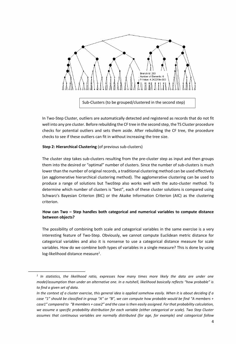
Step 1: Pre-clustering (with an optional Outlier handling): From individuals to small clusters

We will group individuals in a number of intermediate small groups called “pre-clusters”. The goal

of pre clustering is to substantially reduce the size of initial elements/records and thus the

dimension the matrix that contains distances between all possible pairs of “N” cases. When pre

clustering is complete, all cases in the same pre cluster are treated as a single entity. The size of

the distance matrix is no longer dependent on the number of cases but on the number of pre

clusters.

The pre-cluster step uses a sequential clustering approach. It scans the data records one by one

and decides if the current record should be merged with the previously formed clusters or starts

a new cluster based upon its similarity to existing nodes and using the distance measure as the

similarity criterion (Log-Likelihood Distance or Euclidean Distance).

4

In Two-Step Cluster, outliers are automatically detected and registered as records that do not fit

well into any pre cluster. Before rebuilding the CF tree in the second step, the TS Cluster procedure

checks for potential outliers and sets them aside. After rebuilding the CF tree, the procedure

checks to see if these outliers can fit in without increasing the tree size.

Step 2: Hierarchical Clustering (of previous sub-clusters)

The cluster step takes sub-clusters resulting from the pre-cluster step as input and then groups

them into the desired or “optimal” number of clusters. Since the number of sub-clusters is much

lower than the number of original records, a traditional clustering method can be used effectively

(an agglomerative hierarchical clustering method). The agglomerative clustering can be used to

produce a range of solutions but TwoStep also works well with the auto-cluster method. To

determine which number of clusters is "best", each of these cluster solutions is compared using

Schwarz's Bayesian Criterion (BIC) or the Akaike Information Criterion (AIC) as the clustering

criterion.

How can Two – Step handles both categorical and numerical variables to compute distance between objects?

The possibility of combining both scale and categorical variables in the same exercise is a very

interesting feature of Two-Step. Obviously, we cannot compute Euclidean metric distance for

categorical variables and also it is nonsense to use a categorical distance measure for scale

variables. How do we combine both types of variables in a single measure? This is done by using

log-likelihood distance measure1.

1 In statistics, the likelihood ratio, expresses how many times more likely the data are under one

model/assumption than under an alternative one. In a nutshell, likelihood basically reflects “how probable” is

to find a given set of data.

In the context of a cluster exercise, this general idea is applied somehow easily. When it is about deciding if a

case “1” should be classified in group “A” or “B”, we can compute how probable would be find “A members +

case1” compared to “B members + case2” and the case is then easily assigned. For that probability calculation,

we assume a specific probability distribution for each variable (either categorical or scale). Two Step Cluster

assumes that continuous variables are normally distributed (for age, for example) and categorical follow

Sub-Clusters (to be grouped/clustered in the second step)

5

3.- Setting Two – Step & K-Means using IBM-Modeler

Setting a K-Means modeling node in Modeler

1. Before adding a downstream K-Means modeling node, it is recommended to add a TYPE

node to ensure that our data are fully instantiated and to eventually select the variables

to be considered as “inputs” in our analysis

2. Then, we will add a K-Means modeling node. If we have previously selected clustering

variables, we don’t need to specify any custom setting in the “fields” tab.

multinomial distributions (for gender, for example). It is also assumed that the variables are independent of

each other, and so are the cases.

Similarly, the distance between two clusters is related to the decrease in (log) likelihood as they are combined

into one cluster when compared with the likelihood before merging groups. When two groups A and B are more

similar than other alternative combinations (A+C or C+B), the combined group, produces a small variation of

total log likelihood (a greater increase in natural likelihood). The greater the log likelihood variation, the grater

the distance.

Data are fully instantiated

INPUT variables have beenpreviously selected

6

3. Eventually, we might add a partition field/variable. Partition refers to randomly split the

set of records in the database in (at least) two parts. The first part (called “training”

sample) is used to run the algorithm and get the model and the second one (called

“testing” sample) is used to test the model. By using one sample to get the model output

and a separate sample to test it, you can get a realistic indication of how well the model

will generalize to other datasets.2

4. In the “model” tab, we basically set the number “k” of clusters to get. It is impossible to

have a clear idea in advance so we will try different values evaluating the quality of

different clusters results (we discuss about quality in the first document about Cluster

basics)

2 Partition variable, is a special field you create in Modeler using a Partition Node (in “Fields op” tab). Using this

node before your modelling nodes, Modeler automatically generates a nominal field with the role set to

Partition that you can select later in your “partition” option. Alternatively, if you have your own field with your

own partition, it can be designated as a partition variable (any instantiated nominal field with two or three

values can be used as a partition).

When you tried to set a partition variable in your exercise (using the option), Modeler only used a subset of your

data to run the cluster (if you used a partition variable with values 1 and 2, for example, Modeler uses only

cases “1” as training subsample). Obviously, your results for the entire sample may differ (a bit or a lot) of those

you get with a subsample.

Clustering Fields already selectedin the previous TYPE node

A specific partition variable/fieldmight be selected

Number of clusters to get

7

5. Finally, in the expert tab, we set the technical parameters for the iterative K-means

procedure. This is not very common given that a change may produce unpredictable

results; the defaults are usually satisfactory, but if not, you might first try increasing the

number of iterations to get a different clustering solution. The default setting combines

both the change and iterations so that training stops when either the change threshold

or iteration number is reached.

6. The encoding value is a technical parameter that help us to reduce the importance of

categorical variables when mixed with scale variables. Normally, Two-Step is used when

we mix categorical and scale variables, but K-means can also produce a solution if we add

categorical fields in our settings. Given that K-Means uses Euclidean distance, Modeler

cannot use categorical variables as they are coded, so it previously transform categorical

variables into 0/1 Flag variables. Each category of an original categorical field will have a

new temporary input field assigned to it, coded as either 0 or 1, a dummy variable.

Therefore, a categorical field with three values will have three new inputs. However, if

the new inputs are coded with a value of 1, they will tend to dominate the cluster solution

compared to numeric fields. Accordingly, the value of .70711 is used instead. 0.70711

squared = .5, therefore records having a different category will have a distance of .5 + .5

= 1. The Encoding value for sets value can be set between .0001 and 1.0, inclusive. Values

below 0.70711 will decrease the importance of categorical fields, while values above that

will do the reverse.

7. About outliers detection. K-means does not provide an automated outliers detection

mechanism (such as Two-Step). In that sense, remember that the Anomaly node can also

be used before running a cluster analysis. This node provides this capability isolating

records that are far from the cluster centers, or norms, helping us to easily detect

anomalous data, specially when we use categorical data as cluster inputs3.

Setting a Two-Step modeling node in Modeler

3 When we use scale variables, outliers can be easily detected using a simple statistical analysis but when we use categorical data, the definition of “outlier” is not possible in relation to every single variable; the idea is to change the focus looking for anomalous combinations of categories for a set of categorical variables.

We may control the parameters of K-Means iterative process

This value reduces the importance of categorical variables compared to saclevariables.

8

1. As in the case of K-Means, it is recommended to add a TYPE node to ensure that our data

are fully instantiated and to eventually select the variables to be considered as “inputs”

in our analysis. Then, we will add a Two-Step node and specify settings in the “fields” tab

as we previously described for K-Means. Again, we might add a partition field/variable if

desired.

2. In the “model” tab, we decided on three issues:

a. The number of clusters to get if we have a clear idea or we let Two-Step to

automatically select the number of clusters in a given range.

b. We also select if we want to standardize our input fields. This means that they

will have a mean of 0 and a standard deviation of 1. The reason for this

transformation is that Euclidean distance is used by K-Means to calculate

distances and this can cause a problem when fields with widely differing ranges

and standard deviations are used preventing numeric fields with large variances

from dominating the solution.

c. Finally, the exclude outliers option will exclude those clusters with a relatively

small number of records during the first step of cluster formation. Outlier

detection occurs during the preclustering step: subclusters with few records

relative to other subclusters are considered potential outliers. The parameter

controls the size (in Percentage ) below which subclusters are considered to

contain potential outliers is controlled by the option. Potential outliers that

cannot be merged with other groups at the end of clustering are considered

outliers and are added to a "noise" cluster with the name -1.

INPUT variables have beenpreviously selected

Data are fully instantiated

Clustering Fields already selected in theprevious TYPE node

A specific partition variable/field might be selected

9

4.- Interpretation of Modeler output for Two – Step & K-Means

Modeler uses the same interface with the same structure and results either for Two-Step, K-Means or

Kohonen network cluster. The output viewer is divided in different sections offering valuable

information to interpret our clustering outcome:

Model SUMMARY (LEFT hand window)

Algorithm used

Number of input variables and clusters

Cluster (technical) quality: Various measures are used to quantify the "goodness"

of a cluster solution. In a good cluster solution, the elements within a cluster are

similar to one (cohesive) while the clusters themselves are quite different

(separated). A popular measure is the silhouette coefficient, which is a measure of

Automatic selection of clusters

Standardization

10

both cohesion and separation. The silhouette measure ranges from –1 to +1.4 In a

good solution, the within-cluster distances are small and the between-cluster

distances are large, resulting in a silhouette measure close to the maximum value

of 1.

Cluster SIZES (RIGHT hand window)

Size of clusters: There is no a specific rule concerning the minimum number of cases

in a cluster but, to be useful, clusters should not be too small in size and contain

only a few cases. If you find clusters that are too small, you can rerun the analysis,

requesting a solution with fewer clusters, combine downstream the small clusters

with others that are similar, drop small clusters from the solution. Remember that

if you use the TwoStep node, it has an option to exclude outliers: this will exclude

records in very small clusters from the cluster solution

Clusters VIEW (LEFT hand window)

Basically, the cluster output should be used to characterize distinguish and describe each group.

The basic tool we have in the output viewer for that task is the view option in the bottom left

dropdown menu of LEFT window that gives us access to change to “Clusters”view.

Notice that the clusters (1,2,3….) are not shown in numerical order, but in size

order.

Several options are available to represent information in different ways for each

cluster (tables, distribution graphs,…).

Basically, each column shows the information of each cluster. Each cell in the

column describes the average value of clustering variables within each cluster (or

the modal category for categorical variables).

Blue color strength help us to understand the relative importance of each variable

in the segmentation process. In the default setting, fields share the same color for

every cluster because the color intensity shows the overall importance of that field

4 The silhouette measure averages, over all records, (B−A) / max(A,B), where A is the record’s distance to its cluster center and B is the record’s distance to the nearest cluster center that it doesn’t belong to. A silhouette coefficient of 1 would mean that all cases are located directly on their cluster centers. A value of −1 would mean all cases are located on the cluster centers of SPSS Two-Step Cluster Algorithm (for a combination of categorical and continuous variables) some other cluster. A value of 0 means, on average, cases are equidistant between their own cluster center and the nearest other cluster.

11

for the cluster output (as a whole, NOT FOR THE GROUP). As shown in the

illustration below we may change to “within cluster importance” to reveal the

importance of each field in the definition of every single cluster:

By selecting a specific “cell” for a given cluster, the right panel displays the graphical

distribution of this variable into that cluster (dark shadow) compared with the distribution

for the entire dataset. This may help us to distinguish cluster features from overall data

sample.

Variables are ordered (and colored) by overall importance for the cluster solution.

Variables are ordered (and colored) by the importance INSIDE each cluster.

Clusters are sorted from left to right by cluster size but another ordering options are available.

SPSS displays the values of each variable in the “center” of each group or the graphical distribution of the variable compared to the overall distribution.

12

Clusters Comparison:

Appart from comparing each group with the whole sample, the most effective way of describing

each group is to by comparing it with other particular group/s.

By selecting two or more clusters in the left panel (click and then shift click on the cluster

number) we can easily compare the clusters examining the distribution of features across

them.

For continuous features, you see a boxplot for all of the data with superimposed boxplots for

each of the clusters. Be careful to NOTICE that values (or boxes) on the right side mean

HIGHER values for the variable/field.

For categorical targets, there's a dot for each cluster that corresponds to the modal category

shown on the axis. (If you place the cursor on the dot, you'll see the modal category

description and the percent of cases in the cluster that fall into the modal category.) The size

of the dot corresponds to the number of cases in the modal category.

Exploring the output in our dataset

When you run a stream containing a CLUSTER modeling node, the node adds two new fields

containing the cluster membership and distance (only for K-means) from the assigned cluster center

for that record.

• The field SERVICE satisfaction is the most DISCRIMINANT one because (1)modal category is different across groups AND (2) the % of group memberswithin each group (size of spheres) is important.

• For each COLOR (group), therelative size of different globesreveals the relative importanceof each field WITHIN thegroup.

13

It is very common to use this output to further analyze differences between groups, or to investigate

relationship between this grouping variable and a target of interest, or to use that grouping as a split

variable in a subsequent analysis (for example, you may apply a different predictive C5 tree for each

group).

Using “generate” menu from output viewer

Additionally, using “generate” menu from Cluster Viewer, Modeler helps us to generate the

following elements:

Generate Modeling Node. Creates a modeling node on the stream canvas. This would be

useful, for example, if you have a stream in which you want to use these model settings but

you no longer have the modeling node used to generate them.

Model to Palette. Creates the nugget on the Models palette. This is useful in situations where

a colleague may have sent you a stream containing the model and not the model itself.

Filter Node. Creates a new Filter node to filter fields that are not used by the cluster model,

and/or not visible in the current Cluster Viewer display. If there is a Type node upstream from

this Cluster node, any fields with the role Target are discarded by the generated Filter node.

Filter Node (from selection). Creates a new Filter node to filter fields based on selections in

the Cluster Viewer. Select multiple fields using the Ctrl-click method. Fields selected in the

14

Cluster Viewer are discarded downstream, but you can change this behavior by editing the

Filter node before execution.

Select Node. Creates a new Select node to select records based on their membership in any

of the clusters visible in the current Cluster Viewer display. A select condition is automatically

generated.

Select Node (from selection). Creates a new Select node to select records based on

membership in clusters selected in the Cluster Viewer. Select multiple clusters using the Ctrl-

click method.

Derive Node. Creates a new Derive node, which derives a flag field that assigns records a

value of True or False based on membership in all clusters visible in the Cluster Viewer. A

derive condition is automatically generated.

Derive Node (from selection). Creates a new Derive node, which derives a flag field based on

membership in clusters selected in the Cluster Viewer. Select multiple clusters using the Ctrl-

click method.