Current Account Deficit Sustainability: The Case of Barbados

By

Kevin Greenidge1

(Chief Research Economist)

Carlos Holder(Deputy Governor)

Alvon Moore1

(Research Officer)

Abstract

This paper investigates the sustainability of the current account deficit in

Barbados over the period 1960 to 2006. Various unit root and cointegration

techniques are employed to determine whether the country is satisfying its

intertemporal budget constraint. The cointegration regressions suggest

that the current account of Barbados is sustainable and that deviations

from long-run equilibrium between real exports and imports are corrected in

the short-run with imports making the adjustment.

JEL Classification: F30; F32

Key words: Current account deficits; Sustainability; Intertemporal Budget

Constraint1Corresponding Author: Central Bank of Barbados, Toms Adams Financial Centre, Bridgetown, Barbados, Phone: 246 436870, Fax: 246 4271431, Email kcgreenidge@centralbank.org.bb

1

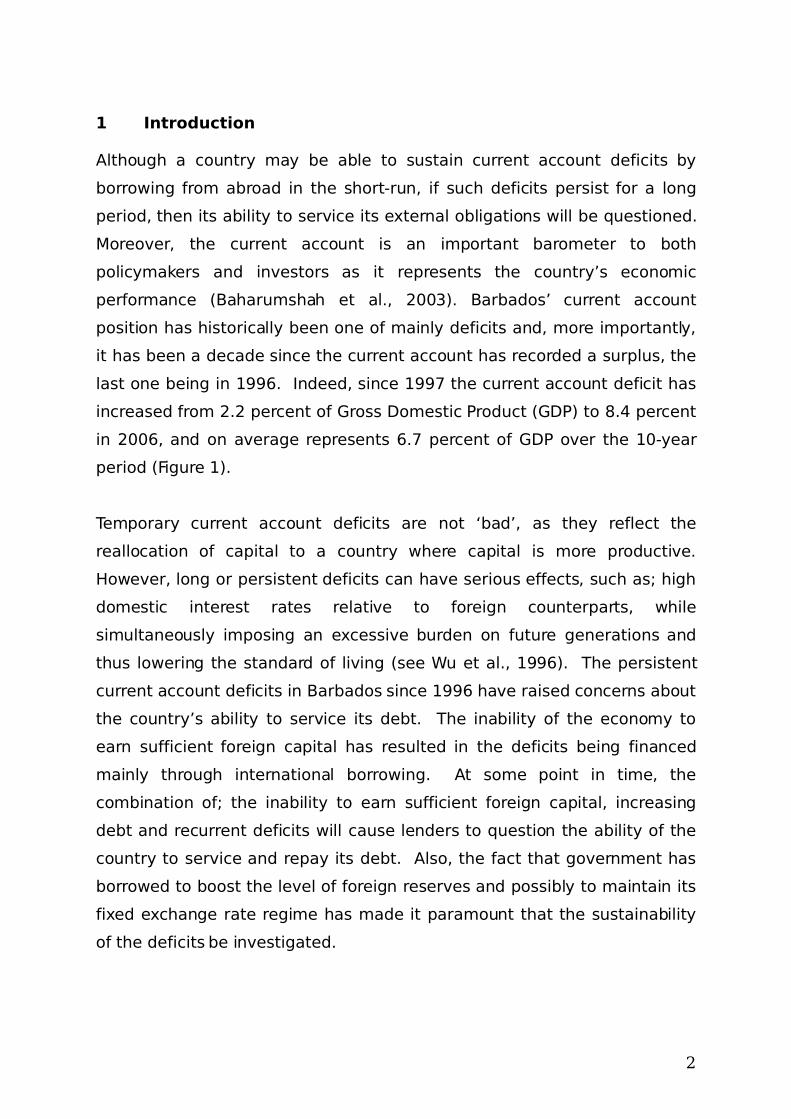
1 Introduction

Although a country may be able to sustain current account deficits by

borrowing from abroad in the short-run, if such deficits persist for a long

period, then its ability to service its external obligations will be questioned.

Moreover, the current account is an important barometer to both

policymakers and investors as it represents the country’s economic

performance (Baharumshah et al., 2003). Barbados’ current account

position has historically been one of mainly deficits and, more importantly,

it has been a decade since the current account has recorded a surplus, the

last one being in 1996. Indeed, since 1997 the current account deficit has

increased from 2.2 percent of Gross Domestic Product (GDP) to 8.4 percent

in 2006, and on average represents 6.7 percent of GDP over the 10-year

period (Figure 1).

Temporary current account deficits are not ‘bad’, as they reflect the

reallocation of capital to a country where capital is more productive.

However, long or persistent deficits can have serious effects, such as; high

domestic interest rates relative to foreign counterparts, while

simultaneously imposing an excessive burden on future generations and

thus lowering the standard of living (see Wu et al., 1996). The persistent

current account deficits in Barbados since 1996 have raised concerns about

the country’s ability to service its debt. The inability of the economy to

earn sufficient foreign capital has resulted in the deficits being financed

mainly through international borrowing. At some point in time, the

combination of; the inability to earn sufficient foreign capital, increasing

debt and recurrent deficits will cause lenders to question the ability of the

country to service and repay its debt. Also, the fact that government has

borrowed to boost the level of foreign reserves and possibly to maintain its

fixed exchange rate regime has made it paramount that the sustainability

of the deficits be investigated.

2

In this regard, the literature suggests several measures of sustainability,

including: the ratio of the country’s foreign indebtedness to GDP, as an

indicator of a country’s ability to service its debt (Krugman, 1989); the real

rate of interest on national debt adjusted for output and population growth

(Cohen, 1988; Cohen and Katseli, 1985; Vinals and Cuddington, 1988); and,

the proportion of foreign net worth held in a particular country’s debt (Isard

and Stekler, 1985). However, the majority of recent works on sustainability

advocate using an intertemporal budget approach, which is basically

assessing whether or not a nation is satisfying its budget constraint over a

defined time period. Wickens and Uctum (1993) suggest that a country

with initial net national indebtedness will satisfy its intertemporal budget

constraint (IBC) if it has future current account surpluses that are expected

to be sufficient to service and repay its debt, or if it has sufficient initial net

national assets to offset expected future current account deficits.

Section 2 traces the current account developments in Barbados during the

period 1966 to 2006. Section 3 provides the theoretical background, while

section 4 outlines the econometric methodology. Section 5 provides the

results and analysis and section 6 concludes the paper and offers some

policy implications.

2. Current Account Developments in Barbados

Barbados’ current account position has fluctuated over the years,

characterised predominantly by longer periods of deficits. The period

between the 1970’s and 1980’s marked the transition of Barbados’

economy from an agricultural and manufacturing base economy to one of

tourism. The export of sugar was the main source of foreign exchange up

to the 1960s. However, poor management, stagnant world sugar prices and

rising production cost eroded the profitability of the industry and eventually

led to its decline. Brathwaite and Codrington (1982) note that the decline of

sugar was sharpest in the 1967 to 1972 period. Growth in the

3

manufacturing and tourism industries however partially compensated but

generated a substantial requirement for imports.

Tourism eventually replaced sugar as the major foreign exchange earner,

but soon suffered a severe blow in the early 1970s, as a result of rising oil

prices and air transport cost coupled with recession in the world economy.

Thus, the years 1971 to 1976 were a period of real economic decline,

marked by increasing current account deficits. Attempts at diversification,

aided by government incentives for manufacturing and import trade

restrictions, help to boost the light manufacturing industry (Hilaire, 2000).

Increased manufacturing output along with a recovering tourist industry

saw the deficit improve between 1977 and 1980.

The slide in sugar profitability continued into the 1980’s, while tourism

output began to decline due to external forces, mainly a fall-off in global

tourist travel. At the same time, recessions in the United States and United

Kingdom led to a drop in merchandise exports, however imports continued

to grow as a result of higher international fuel prices. The poor performance

of the traditional foreign currency earning sectors caused the deficit to

worsen in 1981, by more than five times the previously recorded value. This

placed additional pressure on the foreign reserves. Consequently, the

country was forced to seek funding from the International Monetary Fund

(IMF) in 1982. The ensuing structural adjustment program involved wage

and fiscal restraint, which increased the island’s external competitiveness.

The revival of the world economy, along with the promotion of offshore

financial services helped to improve the economic conditions in Barbados

and propelled the current account position from one of deficit to three

consecutive years of surpluses over the period 1984 to 1986.

The economy moved towards the 90’s with a current account surplus.

However, imports were increasing steadily while exports declined, resulting

in a current account deficit by 1990. The falloff in exports reflected a

faltering manufacturing sector, as the Trinidad and Tobago market

4

contracted, and a drop in the production of electrical components as a

number of large multinational companies such as Intel and CORCOM

relocated their businesses from Barbados in the face of changing

production technologies. In addition, the crisis in the Middle East

culminated in the Gulf War in 1991 and caused a sharp reduction in tourist

expenditure, leading to a further worsening of the current account deficit

(Jordan and Sunielle, 2005). By August of that that year, the reserves had

declined to less than three weeks of imports of goods and services. Again,

this prompted the government to seek funding from the IMF. A reduction in

credit availability along with a cut-back and restructuring in Government

expenditure helped to avoid a possible devaluation of the currency. The

policies aimed at reducing the level of expenditure included a 20 percent

tax increase on luxury imports, 8 percent cut in nominal public sector

wages and lay-offs of 11 percent of public workers. Monetary policy was

also used to dampen credit to the public and private sector; the liquid asset

requirement and minimum deposit rates were raised and the ceiling on loan

rates was removed to discourage borrowing. Collectively, these policies

resulted in a 23 percent decline in imports between 1991 and 1992, while

the fiscal deficit as a percentage of nominal GDP also decreased by about 6

percentage points during the same period. Consequently, the current

account moved from a deficit of 1.3 percent of GDP in 1991 to a surplus of

9.1 percent in 1992. Surpluses were recorded from 1992 to 1997 as

exports along with tourist receipts expanded. The buoyant tourist industry

along with a strengthening private sector, influenced additional spending in

the form of imports, causing the merchandise trade balance to worsen and

by 1997 the current account was again in deficit.

From 1997 to the present period, current account deficit have persisted,

with 2003 being the highest on record. However, this was a period of

increasing economic output led primarily by the non-traded (net foreign

exchange using) sectors and thus much of the imports contributed to the

expansion of the economy. Moreover, during the period 2003 to 2005,

retained imports expanded by 11.5 percent, 17.8 percent and 11.3 percent

5

respectively, however much of this was related to construction activity in

preparation for the hosting of Cricket World Cup 2007. A significant

proportion of the increases in these latter years also reflected an almost

doubling of the fuel import bill in the face of rising international oil prices.

Nonetheless, the current account as a percentage of GDP rose significantly,

moving from 6.8 percent at the end of 2002 to 12.5 percent in 2005.

Presently, the deficit stands at 8.4 percent of GDP as a result of a 7.8

percent decrease in the trade deficit and a 9.0 percent expansion in travel

expenditure.

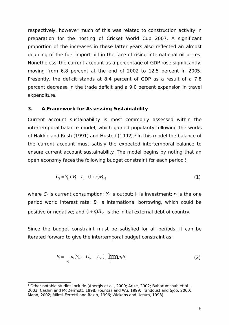
3. A Framework for Assessing Sustainability

Current account sustainability is most commonly assessed within the

intertemporal balance model, which gained popularity following the works

of Hakkio and Rush (1991) and Husted (1992).1 In this model the balance of

the current account must satisfy the expected intertemporal balance to

ensure current account sustainability. The model begins by noting that an

open economy faces the following budget constraint for each period t:

1(1 )t t t t t tC Y B I r B (1)

where Ct is current consumption; Yt is output; It is investment; rt is the one

period world interest rate; Bt is international borrowing, which could be

positive or negative; and 1(1 )t tr B is the initial external debt of country.

Since the budget constraint must be satisfied for all periods, it can be

iterated forward to give the intertemporal budget constraint as:

1

[ ] limt i t i t i t i i ti i

B Y C I B

(2)

1 Other notable studies include (Apergis et al., 2000; Arize, 2002; Baharumshah et al., 2003; Cashin and McDermott, 1998; Fountas and Wu, 1999; Irandoust and Sjoo, 2000; Mann, 2002; Milesi-Ferretti and Razin, 1996; Wickens and Uctum, 1993)

6

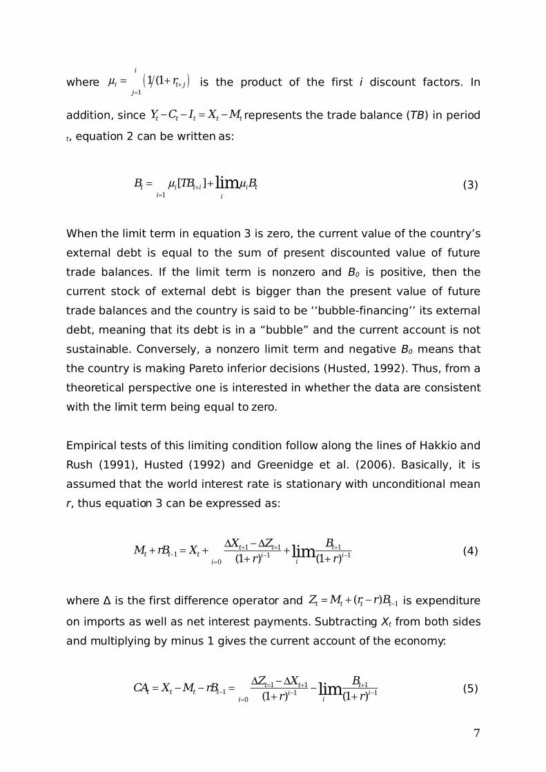
where 1

1 (1i

i t jj

r

is the product of the first i discount factors. In

addition, since t t t t tY C I X M represents the trade balance (TB) in period

t, equation 2 can be written as:

1

[ ] limt i t i i ti i

B TB B

(3)

When the limit term in equation 3 is zero, the current value of the country’s

external debt is equal to the sum of present discounted value of future

trade balances. If the limit term is nonzero and B0 is positive, then the

current stock of external debt is bigger than the present value of future

trade balances and the country is said to be ‘‘bubble-financing’’ its external

debt, meaning that its debt is in a “bubble” and the current account is not

sustainable. Conversely, a nonzero limit term and negative B0 means that

the country is making Pareto inferior decisions (Husted, 1992). Thus, from a

theoretical perspective one is interested in whether the data are consistent

with the limit term being equal to zero.

Empirical tests of this limiting condition follow along the lines of Hakkio and

Rush (1991), Husted (1992) and Greenidge et al. (2006). Basically, it is

assumed that the world interest rate is stationary with unconditional mean

r, thus equation 3 can be expressed as:

1 1 11 1 1

0 (1 ) (1 )limt t tt t t i i

ii

X Z BM rB X

r r

(4)

where Δ is the first difference operator and 1( )t t t tZ M r r B is expenditure

on imports as well as net interest payments. Subtracting Xt from both sides

and multiplying by minus 1 gives the current account of the economy:

1 1 11 1 1

0 (1 ) (1 )limt t tt t t t i i

ii

Z X BCA X M rB

r r

(5)

7

Finally, under the assumption that Xt and Zt are both I(1) processes with

stationary error processes, and that the limit term of Equation 5 approaches

zero, Equation 5 can be written in standard regression format as:

t t tX bMM (6)

where a necessary condition for the country to be satisfying its

intertemporal budget constraint is that εt be stationary, which means that if

X and MM are I(1) then they are cointegrated. However, no cointegration

between X and MM would indicate that the country fails to satisfy its budget

constraint, and is therefore evidence against the sustainability of the

current account balance. The sufficient condition for the intertemporal

budget constraint to be satisfied is the existence of a cointegrating vector

between X and MM of the form (1,-1) such that εt is a stationary process,

implying that the two series would never drift too far apart.

However, the condition b=1 is not, strictly speaking, a necessary condition

for the intertemporal budget constraint to hold. Hakkio and Rush (1991)

showed that when X and MM are in levels, as opposed to a percentage of

GDP or in per capita terms, 10 <<b is a sufficient condition for the budget

constraint to be obeyed, implying current account sustainability.

4. Econometric Methodology

Unit Root Analysis

A first step in testing for cointegration between two variables is to

determine the order of integration of the two series. In this regard, a

battery of stationarity tests is applied to the levels and first differences of

the variables. The first test is that of augmented Dickey-Fuller (ADF) test for

unit roots based on the regressions:

8

1 1 1 11

J

t t t j t j tj

X X X

(7)

and

2 2 2 11

J

t t t j t j tj

MM MM MM

(8)

where J in the regressions is chosen so that it is sufficiently large to ensure

that the error term is free of significant serial dependence. The null

hypothesis of non-stationarity is rejected if )( 21 δδ is significantly negative.

The next test is the Phillips-Perron, PP, (1988) which, instead of adding

differenced terms as explanatory variables to correct for higher order serial

correlation, makes the correction on the t-statistic of the δ coefficient.

However, the PP test, as originally defined, suffers from severe size

distortions when there are negative-moving average errors (see Schwert

1989, and Perron and Ng, 1996). Although the ADF test is more accurate

under such conditions, its power is still affected. In lieu of this we use both

the Elliot, Rothenberg, and Stock (ERS) Point Optimal test (1996), which has

improved power characteristics over the ADF test, and the Ng and Perron

(2001) testing procedure (NP) which exhibits less size distortions compared

to the PP test (both tests are well documented in the literature and are

therefore only summarised in Appendix A).

However, all the above tests take a unit root as the null hypothesis, which

means that they have a high probability of falsely rejecting the null of non-

stationarity when the data generation process is close to a stationary

9

process (Blough, 1992; Harris, 1995). Therefore, we also utilise the KPSS

test described in Kwiatkowski et al.(1992) where the null hypothesis is

specified as a stationary process.

Finally, if there appears to be a shift or structural break in the series then

we need to take account of this as it could distort the above tests. To deal

with this we follow the procedure in Saikkonen and Lütkepohl (2002) and

Lanne et al. (2002), where a shift function is added to the ADF above and

the deterministic term is first estimated by generalised least squares (GLS)

under the unit root null hypothesis and subtracted from the original series.

Then an ADF type test is carried out on the adjusted series which also

includes terms to correct for estimation errors in the parameters of the

deterministic part. The critical values for the new ADF statistic are given in

Lanne et al. (2002). See Saikkonen and Lütkepohl (2000; 2002) for more

details on the specification of the various shift function.

Cointegration Analysis

Johansen cointegration analysis

Once it is established that the two series are I(1) the next step is to test for

the existence of a long-run relationship between them. In this regard, we

rely on the multivariate framework proposed by Johansen (1988) and

Johansen and Jurelius (1990), which is shown to possess several2

advantages over the residual-based Engle-Granger two-step approach. In

conducting the test, consider a vector autoregressive model (VAR) of the

form:

2 See Phillips (1991), Gonzalo (1994) and Johansen and Jurelius (1990) for a further discussions on the advantages of the Johansen procedure.

10

1

p

t t i ti

Y Y

(9)

where ,t tY X MM , η is a 2 1 vector of deterministic variables, Π is a

2 2 coefficient matrix and is a 2 1 vector of disturbances with normal

properties. If there exist a cointegrating relationship between real exports

and real imports then Equation 9 may be reparameterised into a vector

error correction model (VECM):

1

11

p

t i t i t ti

Y Y Y

(10)

where ∆ is the first difference operator, and Φ is an 2 2 coefficient

matrix. The rank, r, of Π determines the number of cointegrating

relationships. If the matrix Π is of full rank or zero, the VAR is estimated in

levels or in first differences respectively, since there is no cointegration

amongst the variables. However, if the rank of Π is less than n then there

exist 2 r matrices β (the cointegrating parameters) and α (the

adjustment matrix, which describes the weights with which each variable

enters the equation) such that βα ′=Π , and Equation 10 provides the more

appropriate framework. The Π matrix is estimated as an unrestricted VAR

and tested to see whether the restriction implied by the reduced rank of Π

can be rejected.

1The test statistics for determining the cointegrating rank of the Π matrix

are the trace statistic given by ∑−=

−−=k

Tiit TQ

1

)1log( λ , for 1,...,1,0 −= kr

and iλ= the thi largest eigenvalue and the maximum eigenvalue statistic,

which is given by 1 1log(1 )t T T TQ T Q Q .

11

Johansen cointegration analysis with structural breaks

If the data and unit root analyses suggest structural breaks then we employ

the test specification and procedure detailed in Johansen et al. (2000).3 The

authors generalised the multivariate likelihood procedure of Johansen

(1988) by allowing up to two structural breaks, either in levels only or in

levels and trend jointly, to be added to the specification.

Assume there are two breaks, in which case the sample can be split into

three periods (q=3) and equation 10 is specified as:

11

, , 11 2 1

p q pt

t t j i j t i t i ti j i t

YY E K D Y

tE

(11)

where tE is a vector of q dummy variables 1, ,( ,... )t t q tE E E with

, 1 ( 1,..., )j tE j q if observation t belongs to the jth period and zero

otherwise, with the first p observations set to zero; and

, 1 ( 2,..., 1,..., )j tD j qand i p is a dummy that equals unity if observation t is

the ith observation of the jth period. The hypothesis for determining the

cointegration rank is formulated as before except that the asymptotic

distribution now depends on the number of non-stationary relationships, the

location of the break points and the trend specification. In this regard, the

critical values as well as the p-values of all Johansen trace tests are

obtained by computing the respective response surface according to

Johansen et al. (2000)4.

Dynamic OLS (DOS) analysis with structural breaks

3 Gregory and Hansen (1996) propose a test for cointegration in the presence of structural breaks by allowing for a level shift, or a shift in both the level and slope. However, it appears that the results depend on the normalisation chosen, and seasonal and short-run dynamics are neglected. 4 This is done using MALCOM 2.9, (available from www.greta.it/malcom/index_malcom.htm ).

12

To ensure the robustness of our results we also utilise the Stocks and

Watson (1993) dynamic ordinary least squares (DOLS), which is an

alternative to the maximum-likelihood estimator of Johansen (1988; 1995),

primarily because it is known to have superior performance in small

samples like ours. Moreover, Stock and Watson (1993) show that the DOLS

estimator is at least asymptotically equivalent to the maximum likelihood

estimator of Johansen (1988) in the case where the variables are I(1). (see

also Caporale and Pittis, 1999; Park and Phillips, 1988; Phillips, 1991;

Watson, 1994). Moreover, the DOLS approach provides unbiased and

asymptotically efficient estimates, even in the presence of endogenous

regressors. It does so by including the leads of the first differences of the

I(1) variables as regressors. It also corrects for serially correlated errors with

the inclusion of the lags of the first differences of the I(1) variables. Thus,

the estimation of the long-run relation for Equation 6 is based on the

following regression:

1

jK

t t j t j i it t tj K i

X bMM MM D MM

(7)

where 1,..., ; 0 (1,... ); 1 ( 1,... )it i it ii J D if t T and D if t T N , where iT is the date

in which the ith identified structural break occurs; and, the inclusion of

t jMM takes care of the possible endogeneity feedback from real exports to

real imports and results in consistent estimates, even under conditions of

two-way exogeneity.5 The equation is estimated in most cases with K=1, but

then a ‘general to specific’ procedure6 is applied to reduce the model to a

more parsimonious congruent specification where only significant variables

are retained.

In order to investigate the short-run dynamics, the estimates from Equation

7 can be used to formulate a general error correction model of the form:

5 See Ahmed and Rogers (1995, pp.361) for further discussion.6 See Campos et al.(2005) for a detailed exposition on the general-to-specific approach to econometric modelling.

13

*1 1

1 0 1 1

p p p j

t j t j j t j j t t i it t tj j j i

X X MM X bMM D MM

(8)

which specifies changes in exports as a function of lagged values of the first

difference of the two nonstationary variables and the stationary

combination of the nonstationary variables, which represents the long-run

relation between exports and imports. This long-run relation is given by b

and is our indicator of current account sustainability, while

*1 1

1

j

t t i it ti

X bMM D MM

can best be interpreted as a measure of current

account disequilibrium and tζ is the speed of adjustment back to

equilibrium. In estimating Equation 8, a general-to-specific approach will be

used in order to reduce it to a more parsimonious representation.

5. Data and Empirical Results

Data

This study uses annual frequency data spanning the period 1960 to 2006.

Consistent with the theoretical framework, exports include exports of goods

and services, while imports is defined as imports of goods and services plus

net transfer payments and net interest payments. Both series are measured

in real terms using the GDP deflator and expressed in natural logarithms.

Data are obtained from the Central Bank of Barbados databank.

It is quite evident from Figure 2 that there is co-movement between the two

series over the sample period. Moreover, this relationship appears to be

relatively steady except from the period, mid-sixties to mid-seventies. Thus,

based on this visual inspection of the two series, we would expect to find

that they are cointegrated. Figure 2 also shows possible structural breaks at

14

the beginning of the 1980s and around 1992, which are consistent with the

discussion in section 2 and will be taken into consideration in the upcoming

analysis.

Results for Unit Root Analysis

The results for the analysis of the stationary properties of the series are

presented in Table 1. All the tests are in agreement and indicate that both

series are non-stationary in levels, )1(I , and stationary in their first

differences, )0(I , at the 1 percent level, for the entire sample.

Given that the possibility of shifts or structural breaks in the series as noted

above, we follow the procedure in Saikkonen and Lütkepohl (2002) and

Lanne et al. (2002), as discussed in the methodology section. In this regard,

instead of using break dates based on our visual inspection we follow Lanne

et al. (2001) and chose a reasonably large AR order and then use a

sequential testing procedure to pick the break date which minimises the

GLS objective function used to estimate the parameters of the deterministic

part. The dates suggested by this procedure coincide with those from our

visual inspection (see Figures 3 and 4).

Figure 3a shows real exports and the resulting shift function for the test

with a break at 1981. The shift function is significant with a t-statistic of

2.867, while the test statistic for the null hypothesis of a unit root with this

function incorporated is -1.378, which is insignificant even at the 10 percent

level. Figure 3b depicts the test for a structural break in exports in 1992.

15

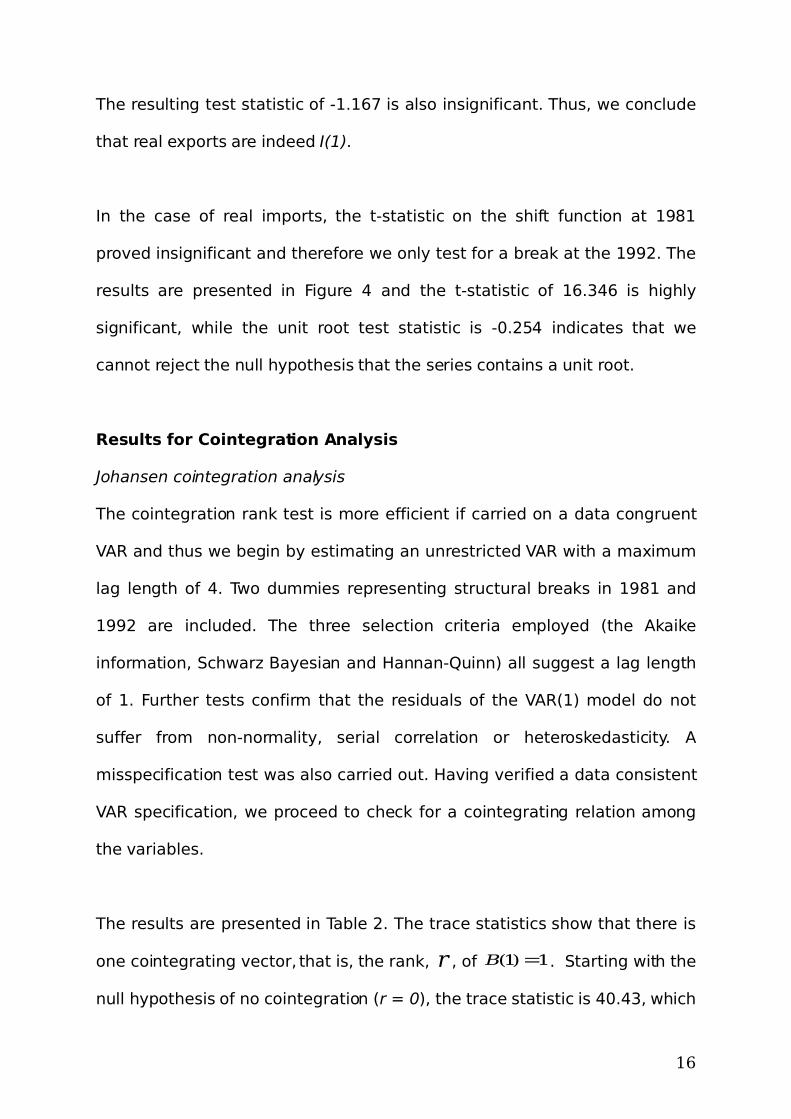
The resulting test statistic of -1.167 is also insignificant. Thus, we conclude

that real exports are indeed I(1).

In the case of real imports, the t-statistic on the shift function at 1981

proved insignificant and therefore we only test for a break at the 1992. The

results are presented in Figure 4 and the t-statistic of 16.346 is highly

significant, while the unit root test statistic is -0.254 indicates that we

cannot reject the null hypothesis that the series contains a unit root.

Results for Cointegration Analysis

Johansen cointegration analysis

The cointegration rank test is more efficient if carried on a data congruent

VAR and thus we begin by estimating an unrestricted VAR with a maximum

lag length of 4. Two dummies representing structural breaks in 1981 and

1992 are included. The three selection criteria employed (the Akaike

information, Schwarz Bayesian and Hannan-Quinn) all suggest a lag length

of 1. Further tests confirm that the residuals of the VAR(1) model do not

suffer from non-normality, serial correlation or heteroskedasticity. A

misspecification test was also carried out. Having verified a data consistent

VAR specification, we proceed to check for a cointegrating relation among

the variables.

The results are presented in Table 2. The trace statistics show that there is

one cointegrating vector, that is, the rank, r , of 1)1( =B . Starting with the

null hypothesis of no cointegration (r = 0), the trace statistic is 40.43, which

16

is well above the 90 percent critical value of 36.1. Hence, it rejects the null

hypothesis r = 0, in favour of the alternative r = 1. However, the null

hypothesis of r ≤ 1 cannot be rejected even at the 10 percent level of

significance. Consequently, we conclude that there is only one cointegrating

relationship between X and MM.

To derive the long-run estimates, an exact identification in sequential order

is imposed. Since there is only one cointegrating vector, this entails first

normalising on MM, then checking the significance of the error correction-

term in the two resulting dynamic equations, then repeating the process by

normalising X. This procedure indicates that the normalisation on MM

produces an error-correction model in which the error-correcting term is

significant only in the MM equation, while with the normalisation on X the

error-correcting term is insignificant in the X equation but significant and

positively signed in MM equation.

Hence, we proceed by normalising on MM and the results are presented in

Table 3 along with some standard diagnostic test statistics for the error

correction model. The estimated long-run relationship is thus 1.086MM X ,

which is highly significant with a t-statistic of 9.274. Note that this implies

that X is weakly exogenous in the cointegrating system with MM responding

to disequilibrium. In other words, short-run deviations from the equilibrium

relationship result in real imports adjusting to restore equilibrium. This is

consistent with the stylised facts in Barbados where, in times of large

current account deficits, policy measures are usually directed at curbing

17

imports in the short-run while various incentives are given to boost exports

in the medium to long-term.

For a sustainable relation, b should be equal to 1 and the results here

suggest that it is not significantly different from 1. Moreover, recursive

estimation7 of the cointegration relationship indicates that it is quite stable

over the sample period (see Figure 5). Thus, the evidence from the

Johansen procedure points to the long-run sustainability of the current

account for Barbados.

Dynamic OLS (DOS)

The final step in our empirical analysis is to further check the robustness of

the above findings by re-estimating the long-run equilibrium relationship

using the DOLS method. The estimation results are reported in Table 4 and

are consistent with those from the Johansen procedure. In addition, the

estimated model is well-behaved and passed the battery of diagnostic tests

(the notes beneath the Table explain the various tests), indicating that it

does not suffer from miss-specification, autocorrelation, heteroscedasticity

or non-normality of the residuals and can therefore be accepted with a high

degree of confidence. Furthermore, testing the restriction of the null

hypothesis that the long-run coefficient parameter b = 1, gives:

2(1) 0.06[ 0.796]p value , which implies that the current account deficit of

Barbados is sustainable.

7 See Greenidge et al. (2006) for an exposition of this procedure as it relates to the sustainability of fiscal deficit.

18

6. Conclusion

The purpose of this study is to investigate the sustainability of the current

account of Barbados by merging the popular Husted (1992) testing

procedure with recent econometric analysis. The procedure utilised here is

to estimate cointegration between exports and imports plus net transfer

payments and net interest payments, allowing for structural breaks.

Cointegration tests based on both the Johansen and DOLS approaches

support the existence of long-run equilibrium between real exports and

imports with a cointegrating factor not significantly different from 1. The

empirical findings therefore suggest that the current account of Barbados

has in fact been sustainable (and does not violate its intertemporal budget

constraint).

Another significant finding is that the stable long-run relationship between

real exports and imports is defined as one where deviations from this

equilibrium are corrected in the short-run with imports making the

adjustment. Thus, policies to curb aggregate demand are effective in

pushing the economy towards achieving external balance in the short-term,

while polices to boost exports are more suited towards the medium and

long-term planning.

The onus is therefore on policymakers to extend this favourable track

record into the future to ensure that future policy decisions continue in the

tradition of prudent current account management that has been

established. This implies that the immediate future requires the current

19

account deficit to be reduced. Of course this is in the face of the new

challenges posed by recent moves to open up the capital account and

deregulate domestic interest rates. It will be necessary to balance the need

for policies which can increase competitiveness and stimulate growth

against the need to maintain external balance in order to preserve

Barbados’ good stability record. One way to achieve this is to integrate

current account targets into the overall framework of macroeconomic

management, whereby policies are designed to ensure that the current

account balances on average over the medium term (roughly a five-year

period).

20

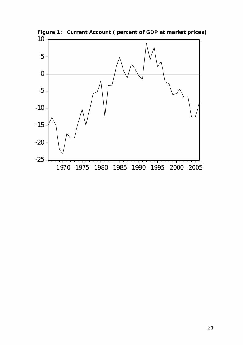
Figure 1: Current Account ( percent of GDP at market prices)

-25

-20

-15

-10

-5

0

5

10

1970 1975 1980 1985 1990 1995 2000 2005

Current Account (% of GDP)

21

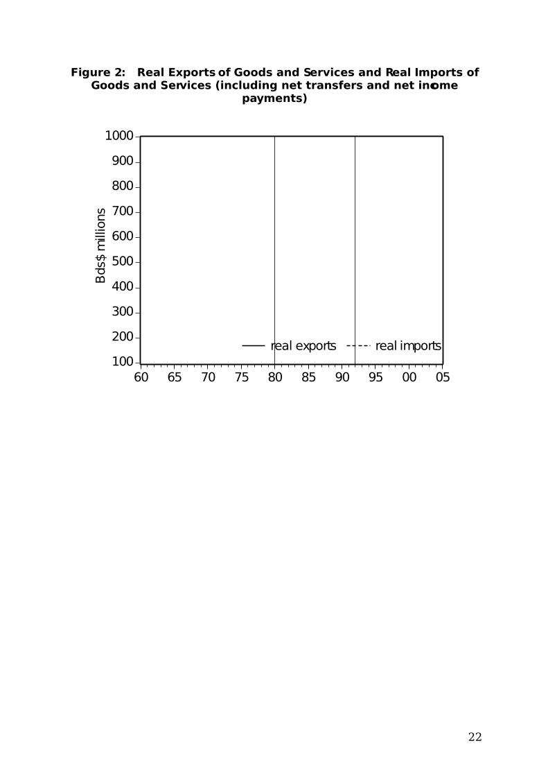
Figure 2: Real Exports of Goods and Services and Real Imports of Goods and Services (including net transfers and net income

payments)

100

200

300

400

500

600

700

800

900

1000

60 65 70 75 80 85 90 95 00 05

real exports real imports

Bds

$ m

illio

ns

22

Figure 3a: Exports – Unit Root Test with Structural Break at 1981

Figure 3b: Exports – Unit Root Test with Structural Break at 1992

Figure 4: Imports – Unit Root Test with Structural Break at 1992

23

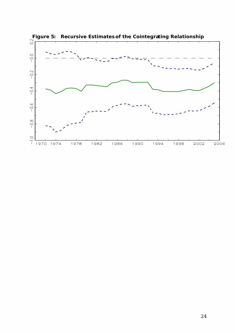
Figure 5: Recursive Estimates of the Cointegrating Relationship

24

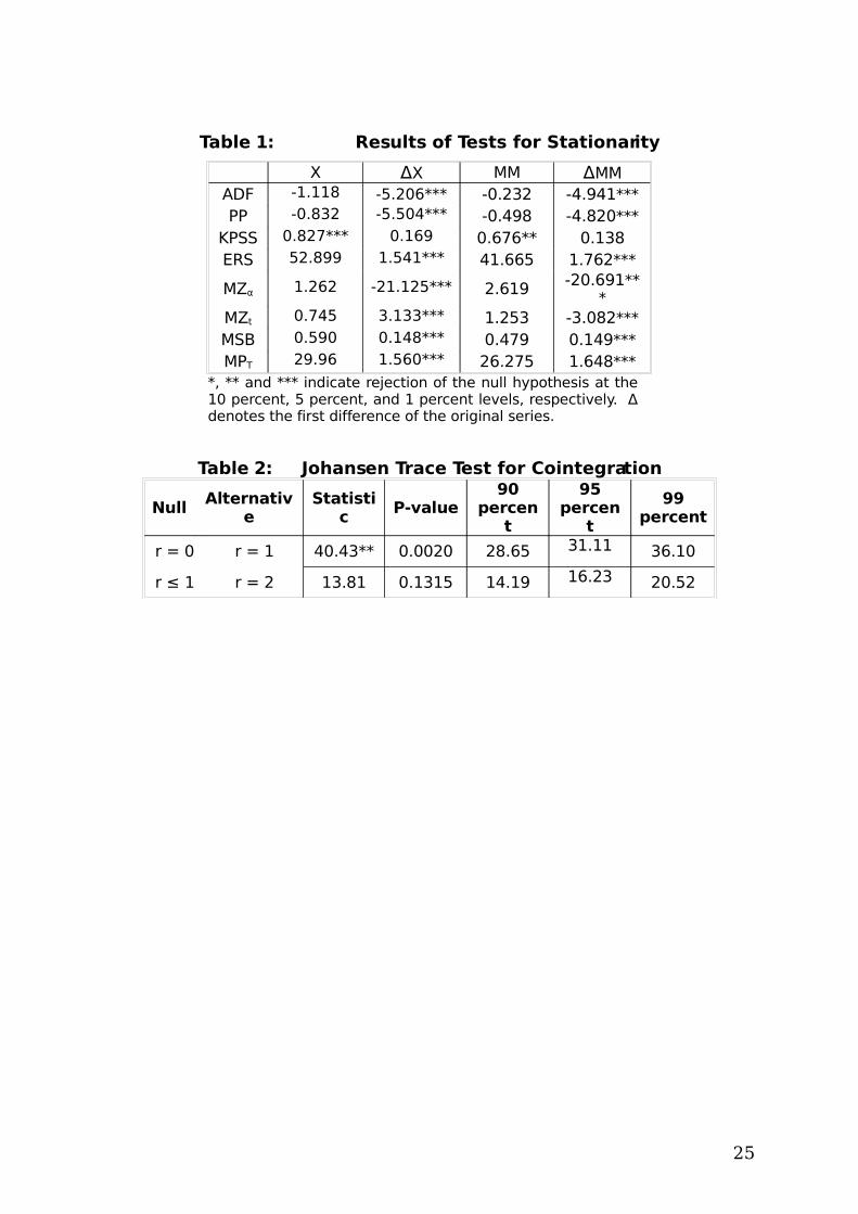
Table 1: Results of Tests for Stationarity

X ΔX MM ΔMMADF -1.118 -5.206*** -0.232 -4.941***PP -0.832 -5.504*** -0.498 -4.820***

KPSS 0.827*** 0.169 0.676** 0.138ERS 52.899 1.541*** 41.665 1.762***

MZα 1.262 -21.125*** 2.619 -20.691***

MZt 0.745 3.133*** 1.253 -3.082***MSB 0.590 0.148*** 0.479 0.149***MPT 29.96 1.560*** 26.275 1.648***

*, ** and *** indicate rejection of the null hypothesis at the 10 percent, 5 percent, and 1 percent levels, respectively. Δ denotes the first difference of the original series.

Table 2: Johansen Trace Test for Cointegration

NullAlternativ

eStatisti

cP-value

90 percen

t

95 percen

t

99 percent

r = 0 r = 1 40.43** 0.0020 28.65 31.11 36.10

r ≤ 1 r = 2 13.81 0.1315 14.19 16.23 20.52

25

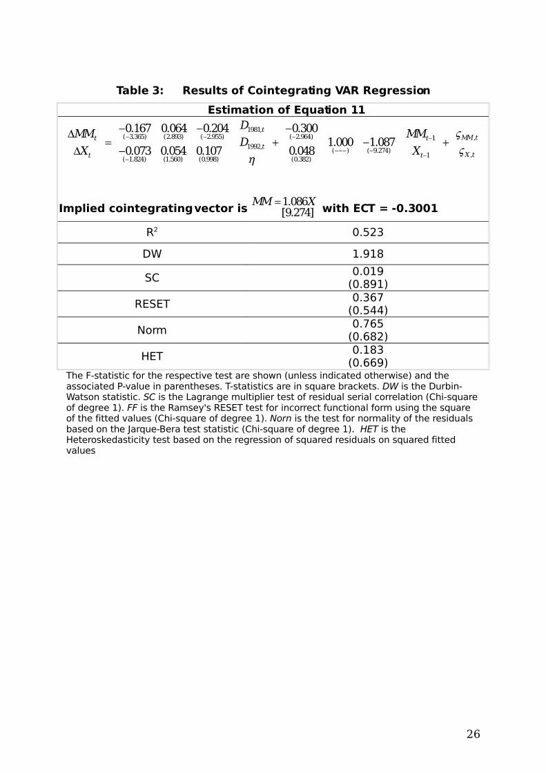
Table 3: Results of Cointegrating VAR Regression

Estimation of Equation 11

1981,( 3.365) (2.893) ( 2.955) ( 2.964) 1

1992,( ) ( 9.274)

1( 1.824) (1.560) (0.998) (0.382)

0.167 0.064 0.204 0.3001.000 1.087

0.073 0.054 0.107 0.048

tt t

tt t

DMM MM

DX X

,

,

MM t

X t

Implied cointegrating vector is 1.086[9.274]

MM X with ECT = -0.3001

R2 0.523

DW 1.918

SC0.019

(0.891)

RESET0.367

(0.544)

Norm0.765

(0.682)

HET0.183

(0.669)The F-statistic for the respective test are shown (unless indicated otherwise) and the associated P-value in parentheses. T-statistics are in square brackets. DW is the Durbin-Watson statistic. SC is the Lagrange multiplier test of residual serial correlation (Chi-square of degree 1). FF is the Ramsey's RESET test for incorrect functional form using the square of the fitted values (Chi-square of degree 1). Norn is the test for normality of the residuals based on the Jarque-Bera test statistic (Chi-square of degree 1). HET is the Heteroskedasticity test based on the regression of squared residuals on squared fitted values

26

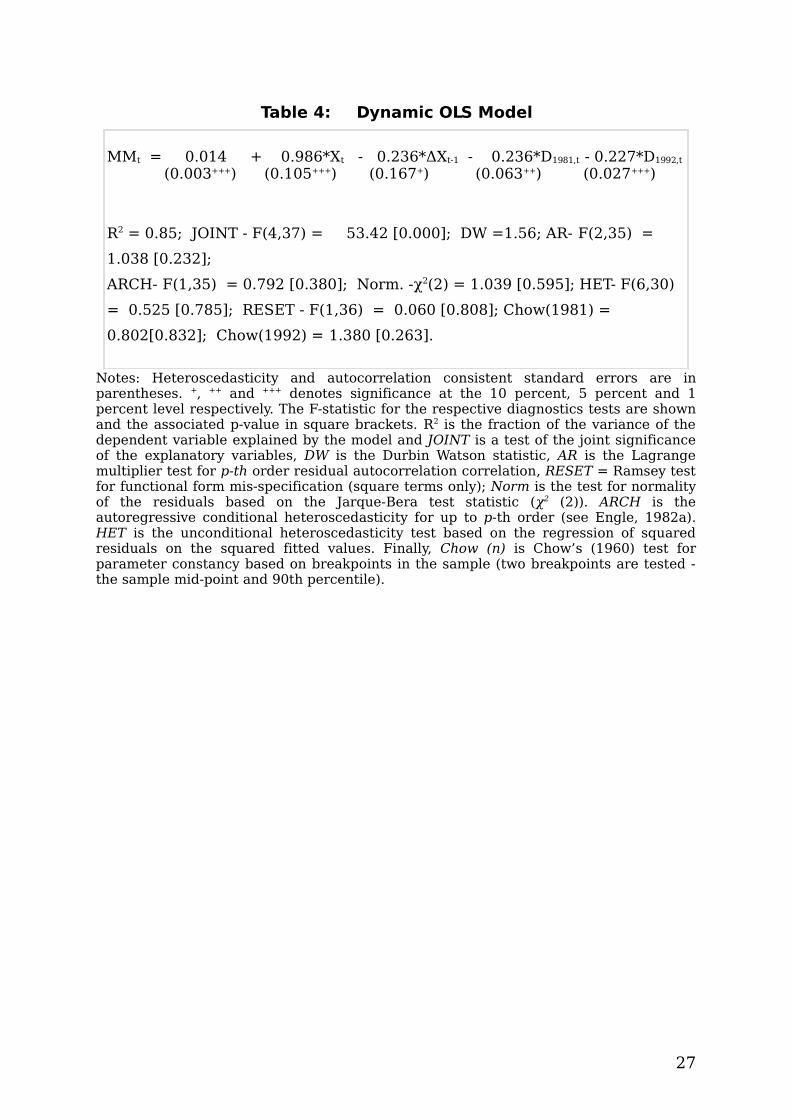
Table 4: Dynamic OLS Model

MMt = 0.014 + 0.986*Xt - 0.236*ΔXt-1 - 0.236*D1981,t - 0.227*D1992,t

(0.003+++) (0.105+++) (0.167+) (0.063++) (0.027+++)

R2 = 0.85; JOINT - F(4,37) = 53.42 [0.000]; DW =1.56; AR- F(2,35) =

1.038 [0.232];

ARCH- F(1,35) = 0.792 [0.380]; Norm. -χ2(2) = 1.039 [0.595]; HET- F(6,30)

= 0.525 [0.785]; RESET - F(1,36) = 0.060 [0.808]; Chow(1981) =

0.802[0.832]; Chow(1992) = 1.380 [0.263].

Notes: Heteroscedasticity and autocorrelation consistent standard errors are in parentheses. +, ++ and +++ denotes significance at the 10 percent, 5 percent and 1 percent level respectively. The F-statistic for the respective diagnostics tests are shown and the associated p-value in square brackets. R2 is the fraction of the variance of the dependent variable explained by the model and JOINT is a test of the joint significance of the explanatory variables, DW is the Durbin Watson statistic, AR is the Lagrange multiplier test for p-th order residual autocorrelation correlation, RESET = Ramsey test for functional form mis-specification (square terms only); Norm is the test for normality of the residuals based on the Jarque-Bera test statistic (χ2 (2)). ARCH is the autoregressive conditional heteroscedasticity for up to p-th order (see Engle, 1982a). HET is the unconditional heteroscedasticity test based on the regression of squared residuals on the squared fitted values. Finally, Chow (n) is Chow’s (1960) test for parameter constancy based on breakpoints in the sample (two breakpoints are tested - the sample mid-point and 90th percentile).

27

Appendix A: The Elliot, Rothenberg, and Stock (ERS) Point Optimal and Ng and Perron tests

The ERS based on a quasi-differencing regression of the form:

( ) ( ) ( )t t td y a d x a a

where yt is the series in question, xt may contain a constant only or both a

constant and a time trend, and a is proxied by a which is computed as

1 7/ 1 13.5/a T and a T in the presence of a constant and a constant and

time trend respectively. The ERS point optimal test statistic of the null that

1 against the alternative that a is given by 0( ) (1) /TP SSR a aSSR f

where SSR is the sum of squared residuals and f0 is an estimator for the

residual spectrum at frequency zero. In making inferences, the test statistic

calculated is compared with the simulation based critical values of ERS.

The NP procedure involves four test statistics. The first calculates the ERS

point optimal statistic for the GLS detrended data ( (̂ )dt t ty y x a ) as:

2 22 2 11 0

1

2 22 2 11 0

1

/ { tan }

(1 ) / { tan , }

Td dt T t

tdT T

d dt T t

t

c T y cT y f if x cons t

MP

c T y c T y f if x cons t trend

The other three are modifications of the PP statistics (the Z and tZ

statistics of Phillips and Perron and the Bhargava statistic) with corrections

for size distortions in the case of negatively correlated residuals. There are

given as:

28

1 2 2 20 1

2

1/2

2 21 0

2

( ) / 2 ( ) /

( ) /

Td d d

T tt

dt a

Td d

tt

MZ T y f y T

MZ MZ MSB

MSB y T f

29

References

Apergis, N., Katrakilidis, K. P., and Tabakis, N. M. (2000), "Current Account Deficit Sustainability: The Case of Greece", Applied Economics Letters, vol. 7, no. 9, pp. 599-603.

Arize, A. C. (2002), "Imports and Exports in 50 Countries: Tests of Cointegration and Structural Breaks", International Review of Economics and Finance, vol. 11, no. 1, pp. 101-115.

Baharumshah, A. Z., Lau, E., and Fountas, S. (2003), "On the Sustainability of Current Account Deficits: Evidence from Four ASEAN Countries", Journal of Asian Economics, vol. 14, no. 3, pp. 465-487.

Blough, S. R. (1992), "The Relationship between Power and Level for Generic Unit Root Tests in Finite Samples", Journal of Applied Econometrics, vol. 7, no. 3, pp. 295-308.

Braithwaite, A. and Codrington, H. (1982), "The External Sector of Barbados: 1946 - 1980," in The Economy of Barbados: 1946-1980, D. Worrel, ed., Central Bank of Barbados: Bridgetown, pp. 141-167.

Campos, J., Ericsson, N. R., and Hendry, D. F. (2005), "General-to-specific Modeling: An Overview and Selected Bibliography", International Finance Discussion Paper no. 838, Board of Governors of the Federal Reserve System: USA.

Caporale, G. M. and Pittis, N. (1999), "Efficient Estimation of Cointegrating Vectors and Testing for Causality in Vector Autoregressions", Journal of Economic Surveys, vol. 13, no. 1, pp. 1-35.

Cashin, P. and McDermott, C. J. (1998), "Are Australia's Current Account Deficits Excessive?", Economic Record, vol. 74, no. 227, pp. 346-361.

Cohen, D. (1988), "How to Reschedule a Heavily Discounted L.D.C. Debt", CEPREMAP Discussion Papers No.8823.

Cohen, D. and Katseli, L. (1985), "How to Evaluate the Solvency of an Indebted Nation", Economic Policy, vol. 1, no. 1, pp. 139-167.

Fountas, S. and Wu, J. l. (1999), "Are the U.S. Current Account Deficits Really Sustainable?", International Economic Journal, vol. 13, no. 3, pp. 51-58.

Greenidge, K., Archibald, X., and Holder, C. (2006), "Debt and Fiscal Sustainability in Barbados," in Finance and Real Development in the Caribbean, A. Birchwood & D. Seeranttan, eds., Caribbean Centre for Monetary Studies, University of the West Indies: St. Augustine, pp. 531-545.

30

Hakkio, C. S. and Rush, M. (1991), "Is the Budget Deficit "Too Large?"", Economic Inquiry, vol. 29, no. 3, pp. 429-445.

Harris, R. I. D. (1995), Using Cointegration Analysis in Econometric Modelling, Prentice Hall/Harvester Wheatsheaf: London.

Hilaire, A. D. L. (2000), "Caribbean Approaches to Economic Stabilisation", IMF Working Papers, WP/00/73.

Husted, S. (1992), "The Emerging U.S. Current Account Deficit in the 1980s: A Cointegration Analysis", Review of Economics and Statistics, vol. 74, no. 1, pp. 159-166.

Irandoust, M. and Sjoo, B. (2000), "The Behavior of the Current Account in Response to Unobservable and Observable Shocks", International Economic Journal, vol. 14, no. 4, pp. 41-57.

Isard, P. and Stekler, L. (1985), "U.S. International Capital Flows and the Dollar", Brookings Papers on Economic Activity, vol. 0, no. 1, pp. 219-236.

Johansen, S. (1988), "Statistical Analysis of Cointegration Vectors", Journal of Economic Dynamics and Control, vol. 12, no. 2/3, pp. 231-254.

Johansen, S. (1995), Likelihood-based Inference in Cointegrated Vector Autoregressive Models, Oxford University Press: New York.

Johansen, S. and Juselius, K. (1990), "Maximum Likelihood Estimation and Inference on Cointegration--With Applications to the Demand for Money", Oxford Bulletin of Economics and Statistics, vol. 52, no. 2, pp. 169-210.

Johansen, S., Mosconi, R., and Nielsen, B. (2000), "Cointegration Analysis in the Presence of Structural Breaks in the Deterministic Trend", Econometrics Journal, vol. 3, no. 2, pp. 216-249.

Jordan, A. and Sunielle, S. (2005), "A Derivation of the Optimal Current Account Balance for Barbados, Jamaica & Trinidad and Tobago", Central Bank of Barbados Working Papers pp. 15-29.

Krugman, P. R. (1989), "Market-Based Debt-Reduction Schemes", Analytical issues in debt.1989 pp. 258-278.

Kwiatkowski, D., Phillips, P. C. B., Schmidt, P., and Shin, Y. (1992), "Testing The Null Hypothesis Of Stationarity Against The Alternative Of A Unit Root: How Sure Are We That Economic Time Series Have A Unit Root?", Journal of Econometrics, vol. 54, no. 1-3, pp. 159-178.

Lanne, M., Lutkepohl, H., and Saikkonen, P. (2002), "Comparison of Unit Root Tests for Time Series with Level Shifts", Journal of Time Series Analysis, vol. 23, no. 6, pp. 667-685.

31

Mann, C. L. (2002), "Perspectives on the U.S. Current Account Deficit and Sustainability", Journal of Economic Perspectives, vol. 16, no. 3, pp. 131-152.

Milesi-Ferretti, G. M. and Razin, A. (1996), "Current Account Sustainability: Selected East Asian and Latin American Experiences", C.E.P.R.Discussion Papers.

Park, J. Y. and Phillips, P. C. B. (1988), "Asymptotic Equivalence of Ordinary Least Squares and Generalized Least Squares in Regressions With Integrated Regressors", Journal of the American Statistical Association, vol. 83, no. 401, pp. 111-115.

Phillips, P. C. B. (1991), "Optimal Inference in Cointegrated Systems", Econometrica, vol. 59, no. 2, pp. 283-306.

Saikkonen, P. and Lutkepohl, H. (2000), "Testing for the Cointegrating Rank of a VAR Process with Structural Shifts", Journal of Business and Economic Statistics, vol. 18, no. 4, pp. 451-464.

Saikkonen, P. and Lutkepohl, H. (2002), "Testing for a Unit Root in a Time Series with a Level Shift at Unknown Time", Econometric Theory, vol. 18, no. 2, pp. 313-348.

Stock, J. H. and Watson, M. W. (1993), "A Simple Estimator of Cointegrating Vectors in Higher Order Integrated Systems", Econometrica, vol. 61, no. 4, pp. 783-820.

Vinals, J. M. and Cuddington, J. T. (1988), "Fiscal Policy and the Current Account: What Do Capital Controls Do?", International Economic Journal, vol. 2, no. 1, pp. 29-37.

Watson, M. W. (1994), "Vector Autoregressions and Cointegration," in Handbook of Econometrics, Volume 4 edn, F. E. a. D. Robert, ed., Elsevier: pp. 2843-2915.

Wickens, M. R. and Uctum, M. (1993), "The Sustainability of Current Account Deficits: A Test of the U.S. Intertemporal Budget Constraint", Journal of Economic Dynamics and Control, vol. 17, no. 3, pp. 423-441.

Wu, J. l., Fountas, S., and Chen, S. l. (1996), "Testing for the Sustainability of the Current Account Deficit in Two Industrial Countries", Economics Letters, vol. 52, no. 2, pp. 193-198.

32