Currency Crisis Models for Emerging Markets

By

Peter J.G. Vlaar∗

January 2000

Abstract:

In this paper, a new method is introduced to predict currency crises. The method models a continuouscrisis index based on depreciations and reserve losses. The fact that during currency crises, thebehaviour of market participants differs from normal circumstances is modelled by means of modelwith two regimes, one for troubled, and one for normal times. Both the probability of entering thecrisis regime, and the expected depreciation and volatility in this regime depend on economiccircumstances. The probability of crisis can be explained by the real exchange rate, the inflation rate,the growth of the short-term debt over reserves ratio, the reserves over M2 ratio, and the imports overexports ratio. The depth of a crisis is primarily related to local depreciations and the short-term debtover reserves ratio. The most important factors for explaining current month’s crisis index are recentchanges in the exchange rate and reserves themselves however. The model is reasonably successful inpredicting currency crises, also out of sample.

Keywords: Panel data, endogenous jumps, two regime econometric model, fundamentals

Jel Codes: C49, F31, F34

∗ Econometric Research and Special Studies Department, De Nederlandsche Bank, p.o. box 98,1000 AB Amsterdam, The Netherlands. Tel +31 20 524 3189, Fax +31 20 524 25 29, e-mailp.j.g.vlaar@dnb.nl. I thank Peter van Els and seminar participants at De Nederlandsche Bank and theAutumn Meeting of Central Bank Economists at the BIS for valuable comments and discussions.

- 1 -

1 INTRODUCTION

In recent years, the frequency of currency crises in developing countries seems to have increased.

Moreover, the consequences of these financial crises have probably worsened, not only for the country

concerned, but also for other countries in the region, due to increased international trade and capital

flows. As a consequence, research on the prediction of currency crises has spurred. In this paper, this

research is summarised and a new approach to modelling currency crises is introduced. Our main goal

will be to identify weaknesses in the economy that have led to currency crises in the past. Knowing the

main vulnerabilities from the past might help to take prompt corrective action to avoid new crises,

especially if these weaknesses materialise sufficiently long before a crisis.

In order to predict currency crises, the definition of a currency crisis is of course essential. In the

theoretical literature, currency crises are only defined for fixed exchange rate regimes. A crisis is

identified as an official devaluation or revaluation, or instances in which the currency is floated. This

definition is probably too strict to be useful for our purposes. Many currency crises involve currencies

that are not formally fixed to one currency or a basket of currencies, but are allowed to float within

certain margins. Even currencies that are allowed to float freely might be subject to a disruptive

depreciation due to a speculative attack. Moreover, a small official devaluation in a tranquil period

does not have to be disruptive as it probably brings the real exchange rate more in line with

fundamentals. Such an action might very well preclude future speculative attacks, and should not be

identified as a crisis. For most purposes, the size of the depreciation is what matters, not so much

whether this depreciation is caused by an official policy move or otherwise. Therefore, many empirical

studies define a currency crisis as a large (either nominal or real) depreciation. Here the problem arises

as to derive the appropriate threshold above which a depreciation should be labelled a crisis. Another

issue concerning the definition of a crisis is whether or not to include unsuccessful speculative attacks.

Authorities may react to a currency attack by means of direct intervention in the foreign exchange

market, or by raising interest rates. These attacks might also be included in the crisis definition as the

necessary policy actions might be disruptive for the economy as well. Also from an investor’s point of

view, including unsuccessful speculative attacks might be useful as unsuccessful attacks also indicate

vulnerability.

In this paper, a currency crisis indicator is constructed for emerging markets, based on monthly

nominal exchange rate depreciations relative to the US dollar and losses of official reserves. Interest

rates are not included in the index as interest rate data for emerging countries are not always available

and/or reliable. The main innovation in our modelling approach is that we model the crisis index itself,

instead of a zero-one variable representing index values below or above a certain threshold. The

proposed model has two regimes -- one for tranquil and one for crisis episodes -- where the probability

of entering the crisis regime depends on the economic circumstances. In the crisis regime, both the

mean depreciation and the volatility are larger. The modelling technique resembles the one introduced

- 2 -

in Vlaar (1998), where a two-regime model was used to predict weekly exchange rate changes within

the European Monetary system, but is extended in two respects. First, not only the probability to enter

the crisis regime, but also the mean depreciation and the volatility in this regime are allowed to differ

with economic circumstances. Second, the model is adjusted to allow for panel data estimation.

The continuous modelling approach has several advantages. First of all, by using the index itself, we

do not throw away information regarding the severity of a crisis. Therefore, large index values have

more impact on the model than values just above the (arbitrarily set) crisis threshold. Second, as the

continuous crisis variable varies between observations, there is no need to include many crisis

episodes in the sample in order to be able to estimate the model. Consequently, we can concentrate on

emerging markets without having to include developed countries in the sample as well. Finally, the

continuous modelling approach allows to distinguish variables that have an effect on the probability of

a crisis from those that affect the severity of crises.

The rest of this paper is organised as follows. In Chapter 2, some theoretical background on currency

crises is given. Chapter 3 summarises the main results from the empirical literature. In Chapter 4, the

new modelling approach is described. Chapter 5 contains the estimation and forecast results, and

Chapter 6 concludes. The appendix describes the data.

2 THEORETICAL CONSIDERATIONS

As to the reasons for currency crises, the ‘first generation’ models of, e.g., Krugman (1979) focus on

inconsistencies between an exchange rate commitment and domestic economic fundamentals, such as

excess creation of domestic credit, typically prompted by a fiscal imbalance. In these models currency

crises necessarily occur because international reserves are gradually depleted. The solution of the

model is such that the remaining reserves before the attack are just enough to satisfy the foreign

currency demands of market participants during the attack. If they should wait longer, they would

certainly lose money.

The ‘second generation’ models of, e.g., Obstfeld (1986) views currency crises as shifts between

multiple monetary equilibria in response to a self-fulfilling speculative attack. Consequently, the

timing of the attack can no longer be determined, as it is no longer unique. In these second-generation

models currency attacks can take place even though current policy is not inconsistent with the

exchange rate commitment. The attacks can nevertheless be successful because the costs of

maintaining a currency peg, in the form of high domestic interest rates, rise in response of the attack.

In this framework, speculative attacks become more likely if high interest rates become more

problematic. One reason for this might be economic slowdown or high unemployment rates. Another

reason might be a weak domestic banking sector (Obstfeld, 1995). Raising interest rates increases

- 3 -

short-term funding costs for banks, whereas the higher proceeds from loans might be dubious due to

the on average longer maturity of loans relative to deposits and the increased probability of bad loans.

This is one way banking and currency crises might be related. If there is an implicit government

commitment to bailout troubled banks, bank runs might also lead directly to a currency crisis if the

increased liquidity which results from the government bailout is inconsistent with the fixed parity

(Velasco, 1987; Calvo, 1998). The causality between banking and currency crises might also run in the

other direction however, for instance if the domestic banking sector is exposed to exchange rate risk

due to short-term foreign lending (Chang and Velasco, 1998). Indeed, Kaminsky and Reinhart (1996)

find evidence of both directions, although during most twin crises, the banking crisis is preceded by

the currency crisis.

An implicit assumption of the second-generation models is that speculators know exactly what other

speculators will do, as the attack will only be successful if they co-ordinate. In the third generation

models, e.g. Morris and Shin (1998), this co-ordination problem is solved by assuming that the exact

state of the fundamentals can only be observed with noise. If the amount of noise in the signal is

known to differ between speculators, a unique equilibrium again exists. Even if all speculators know

that the peg is in accordance with the current level of fundamentals, they might still attack because of

the uncertainty regarding other people’s expectations.

3 EMPIRICAL LITERATURE

Kaminsky, Lizondo and Reinhart (1998) summarise the results of 28 empirical studies on currency

crises that have appeared over the last twenty years. Although the studies differ widely in crisis

episodes considered and methodologies used, some general conclusions can be drawn. First of all, in

order to be able to explain all currency crises a wide variety of variables is needed. This is because

crises can have many different reasons, which can be represented by different economic variables.

Some variables do seem to have predictive power for most of them however. In particular real

exchange rates and international reserves are included in many studies and found significant most of

the time. Other variables that seem to do well, although the limited number of studies considering

them precludes firm statements, are the domestic inflation rate and domestic credit growth. Current

account deficits on the other hand are usually not found to have significant impact. Rather than

replicating the results by Kaminsky et al, we choose to highlight just a few typical studies, thereby

concentrating on emerging markets. The studies will be categorised by methodology used.

- 4 -

3.1 The signal approach

The signal approach is primarily a bilateral method, comparing the incidence of crisis with the value

of one particular economic variable at the time. For each variable the average level (or growth) in the

period preceding the crises is compared to that in tranquil periods. If the variable behaves differently

before a crisis, an extreme value for this variable provides a warning signal. The question what value

should be considered extreme in this context is solved by weighing the percentage of crises predicted

to the percentage of false signals. The threshold level can either be the same for all countries, or be

based on the country specific empirical distribution of the variable. Given the warning signals of the

individual variables, a composite leading indicator can be constructed as a weighted average of the

individual signals.

In this procedure, both the crisis indicator and the explanatory variables are transformed to dummy

variables, indicating a value above or below a given threshold. This procedure probably gives the best

results if there is a clear distinction between crisis episodes and periods of tranquillity. Regarding the

crisis indicator, this is probably true if only the most severe crises are above the threshold or if the

crisis definition is related to a currency peg. However, in most studies the number of severe currency

crisis is limited, and less serious depreciations are also labelled crisis. In that case, there is no clear

distinction between observations that are just above, and those just below the crisis threshold.

Concerning the explanatory variables, disregarding the exact value of the variable seems inefficient as,

for instance, a current account deficit twice the value of the threshold seems to provide a stronger

signal that a deficit just above it. If the individual signals are combined to compute a composite

leading indicator, this inefficiency will probably lead to less optimal results. Another problem that

arises in combining the signals is that the optimal weights for the individual signals can not easily be

assessed if the signals are correlated. If one is primarily interested in finding vulnerabilities however,

without being particularly interested in exact probabilities, this method is most suited. It gives you

immediately the variables that cause the weakness. This is particularly important for finding

appropriate economic policy actions.

Kaminsky, Lizondo and Reinhart (1998) use a signal approach to predict currency crises using

monthly data for a sample of 15 developing and 5 industrial countries during 1970-95. In their study, a

currency crisis is defined to occur when a weighted average of the monthly percentage nominal

depreciation (either in US dollar or D-mark) and the monthly percentage decline in reserves exceeds

its mean by more than three standard deviations for that country.1 For 15 variables, based on

economic priors and data availability, they compare the levels in the 24 months prior to the crises with

1 Weights, mean depreciations and volatility are calculated separately for high inflation episodes, defined as months preceded

by six months with more than 150% inflation.

- 5 -

values in tranquil periods. For each variable, an optimal threshold value is computed, above which the

variable gives a signal for a crisis in the coming 24 months. The threshold levels are computed as a

percentile of the distribution of the variable by country in such a way that the noise to signal ratio is

optimal. The variables that have most explanatory power turn out to be (1) the real exchange rate

deviation from a deterministic trend, (2) the occurrence of a banking crisis (3) the export growth rate,

(4) the stock price index growth rate, (5) M2/reserves growth rate, (6) output growth, (7) excess M1

balances, (8) growth of international reserves, (9) M2 multiplier growth, and (10) domestic credit over

GDP growth rate.

Country specific threshold levels for the economic variables have the advantage that country specific

elements are taken into account. However, as the same percentile is used for all countries, it also

implies that, within sample, all variables signal the same number of crises per country. Although only

countries that experienced currency crises are included in the sample, this artefact seems undesirable.

The real exchange rate is by far the most successful indicator. However, this result might be partly

spurious as the deviation of the bilateral real exchange rate from a deterministic trend is used.

Consequently, any real overvaluation according to this definition has to lead to either a depreciation or

a lower inflation rate at home than in the reference country.

Berg and Pattillo (1998) evaluated their approach to predict the Asian crisis (out of sample), and found

mixed results. Most (68%) crises were not signalled in advance and most (60%) of the signals were

false. Nevertheless, the predictions were better than random guesses, both economically and

statistically. The results improve slightly (also in sample) if the current account relative to GDP and

the level of the M2 to reserves ratio are also included. They also compare the ranking of severity of

currency crises in 1997 with the ranking of vulnerability according to predicted probabilities of crisis.

The composite leading indicator can explain 28 percent of the variance. If the current account to GDP

and M2 to reserve ratios are also included, this percentage rises to 36.

3.2 Limited dependent regressions

In the limited dependent regression models (logit or probit models), the currency crisis indicator is

modelled as a zero-one variable, as in the signal approach. The explanatory variables are not

transformed to dummy variables however, but are usually included in a linear fashion. The logit or

probit functions make sure that the predicted outcome of the model is always between zero and one.

The regression approach has several advantages compared to the signal approach. First of all, the

prediction of the model is easily interpreted as the probability of a crisis. Moreover, as the method

considers the significance of all the variables simultaneously, the additional information of new

variables is easily checked. A disadvantage of this approach might be that the impact of an individual

variable is less easily detected. Due to the non-linear logit or probit function, the contribution of a

particular variable depends on all the other variables as well. A practical problem of this approach for

- 6 -

currency crises is that the number of crises is usually limited. Consequently, there are only a few ones

in the sample, compared to a huge amount of zeros, resulting in poor estimation results. In order to

increase the number of ones, many studies combine industrialised and emerging markets.

Frankel and Rose (1996) use the probit model to estimate the probability of crisis in an annual sample

of 105 developing countries covering 1971-1992. A crisis is defined as a depreciation of at least 25%,

exceeding last year’s depreciation by at least 10%. The use of annual data has the advantage that more

variables are available, for instance regarding fiscal positions and external debt. Moreover, compared

with monthly data, the balance between zeros and ones in the sample is probably better. They find 69

crashes in 780 observations. They present several specifications, and conclude that the probability of

crisis increases when output growth is low, domestic credit growth is high, foreign interest rates are

high, foreign direct investment as a proportion of total debt is low, reserves are low, or the real

exchange rate is overvalued. The results for output growth, the real exchange rate and reserves were

not robust across specifications however. Berg and Pattillo (1998) evaluate the results of Frankel and

Rose. Using a cut-off probability of 25 percent2, only 17 out of 69 crises are rightly predicted within

sample, whereas 33 out of 711 tranquil periods are wrongly predicted. They argue that one of the

reasons for these rather poor results might be that the country group is too diverse. They proceed with

a smaller group of larger (emerging) markets over the sample 1970-1996. Given results in other

studies, the reserves over M2 and the reserves over short-term debt ratios are also included as

explanatory variables, where only the former shows significant results. For this specification, 38 out of

60 crises and 342 out of 383 tranquil periods are rightly predicted. The out-off-sample results are still

disappointing however. According to the definition of Frankel and Rose, there were no crises in 1997!

This clearly indicates one of the problems with yearly data if a crisis takes place around the end of the

year. If the ranking of their crisis index in 1997 is compared with the ranking of predicted probabilities

of crisis, only 6 percent of the variance is explained in the original specification. For the modified

model the percentage is even lower, 5 percent. In both cases the model does not significantly better

than random guesses.

Berg and Pattillo (1998) also use a probit model to estimate currency crises. They base themselves on

the data and crisis definition of Kaminsky et al (1998), augmented by the current account and the ratio

of M2 over reserves, as described above. In their regression model not only the crises themselves are

labelled ‘one’, but also the 23 months prior to the crisis. Economically, this procedure has the

advantage that the optimal model is sought that signals a crises two years in advance. Of course, this

also means that the seeds of a crisis are supposed to be visible two years in advance. Statistically, the

procedure strongly improves the balance between the zeros and the ones in their monthly data set.

2 This means that a warning signal for an upcoming crisis is given if the probability of a crisis is at least 25%.

- 7 -

They investigate whether a threshold value for the explanatory variables, as in the signal approach,

improves on a linear specification. This turns out not to be the case. The variables that have most

explanatory power are (1) the deviation of the real exchange rate from trend, (2) the current account,

(3) reserve growth, (4) export growth, and (5) the ratio of M2 to reserves. In the model, not the

variables themselves, but the percentiles of the country-specific distribution of the variables are

included. Using a cut-off probability of 25%, the model signals 48% of crisis and 84% of tranquil

periods correctly, within sample. Out of sample, the results are even better. 80% of crisis and 79% of

tranquil periods are correctly called. The prediction of the ranking of severity of crisis in 1997 is not

very successful. Only 23% of the variance is explained, slightly worse than the signal approach of

Kaminsky et al. (1998), though still significantly better than random guesses.

The ‘Event Risk Indicator’ by J.P. Morgan (1998) is based on a logit regression on monthly

observations for 25 industrial or emerging countries over the sample 1980-1997. Their crisis indicator

is defined as a monthly real depreciation of the key bilateral exchange rate of over 10%. Consequently,

this crisis definition excludes unsuccessful speculative attacks. As there basic goal is to find a model

that can be used to predict profitable months to invest in weak currencies, this choice is reasonable.

They balance the number of crises and tranquil periods in their sample by including only three tranquil

periods per country. The explanatory variables for these three periods are calculated as follows. First,

the average value of the variables over the estimation sample (1980-1994), excluding the months there

was a crisis, the month before, and the month after these crises. Second, the average plus one standard

deviation over the same sample, and third, the average minus one standard deviation. As a

consequence, the predictions of the model are not directly interpretable a probabilities of a currency

crash. The key factor behind currency crashes is supposed to be lack of competitiveness, included in

the model as an overvalued real exchange rate (a dummy variable that can take the values one to four,

depending on the average value of the real exchange rate in last two years, relative to the average

value in the ten years before). As the model is used to select profitable investment months in weak

currencies, predicting the exact timing of crisis is extremely important. This timing is supposed to

depend on two factors. First, the credibility of the government's commitment to defend the exchange

rate, which is related to expected economic growth (modelled by means of the three-month rise in

stock prices) and the size of foreign exchange reserves (relative to foreign debt). Second, the force of

financial contagion, reflected in global risk appetite and local currency crash clustering. Global risk

appetite is hereby measured as the correlation between returns and risk (reflected in high interest rates

and an overvalued currency) over the last three months. Both the one month lagged and the seven

months lagged six months change in this variable are included as currency crises are most likely if risk

appetite changes from positive to negative. The local currency crashes variable is computed as a

weighted number of currency crises in the relevant currency block (D-mark or dollar) in the last six

months, where recent crashes are given a higher weight than previous ones.

- 8 -

The regression results show that the six months change in risk appetite is the most important

explanatory variable, followed by the number of local crashes and the reserves to debt ratio. The real

exchange rate is just significant at the 5% level, the six-month change in risk appetite lagged seven

months at the 10% level, and the change in stock prices at the 15% level. Using a cut-off level of 40

percent3, 31 out of 37 crisis and 69 out of 74 quiet periods are correctly predicted within sample. Also

out of sample, the model seems to predict quite well, as an investment strategy based on the model

predictions outperforms a passive, or random investment strategy on average. According to the

authors, the results of the model are most sensitive for the clustering variable, followed by the current

and lagged change in risk appetite. Notwithstanding the importance of current sentiment, they also

claim the model signals all the major first crashes, including Mexico (December 1994), the ERM

(September 1992), and Thailand (July 1997). This is surprising as only lagged variables are used in the

model, and some of these crises came as a complete surprise to the market, thereby precluding the

importance of contagion variables.

3.3 Severity of crisis indicators

A third category of models is not directly aimed at predicting the timing of currency crises, but at

predicting which countries are going to be hit hardest, given the occurrence of a crisis somewhere in

the world. If the timing of currency crises is largely unpredictable, for instance due to the importance

of market sentiments, and the behaviour of financial markets during an international crisis is supposed

to be different from normal behaviour, this strategy might be most fruitful. The idea is to define a

crisis index (for instance based on depreciations and international reserve losses), spanning the whole

period international markets were under stress, for a cross-section of countries. The differences

between countries in magnitude of this crisis index are subsequently explained by variables

representing the economic situation at the onset of the crisis. This can be done by simple cross-section

regression analysis. Usually, only one crisis episode is considered at the time, but a panel of crisis

episodes can be used as well.

Sachs, Tornell, and Velasco (1996) use this framework to explain the severity of currency crisis during

the Mexican crisis of December 1994 (the so-called Tequila effect). They examine data on a cross-

section of 20 emerging markets. Their crisis index is defined as a weighted average of the percentage

decrease in reserves and the percentage depreciation of the exchange rate, from November 1994 to

April 1995. They claim that only countries that were already vulnerable were hit by the Mexican

crisis. Only three factors are essential for measuring vulnerability. First, an overvalued real exchange

rate, measured as the real appreciation between the average 1986-89 level and the one over 1990-94.

Second, a weak banking system, measured by the four year growth in credit to the private sector.

3 Over the period January 1988 to September 1997, this cut-off point would signal the risk of a crises 29% of the time.

- 9 -

Third, low levels of international reserves relative to M2. It turns out that only the combination of

weak fundamentals (real overvaluation or weak banks) and relatively low reserves induced a crisis.

They also investigate the influence of investment, savings, current accounts, the size of capital

inflows, and fiscal policy stances, but these variables do not improve the results. Depending on the

window over which the crisis index is calculated, their model can explain 51 to 71 percent of the

variation in the crisis index over the Mexican crisis. Berg and Pattillo (1998) investigate whether the

same equation can explain variation in the severity of crisis during the Asian crisis. Unfortunately this

is not the case. Moreover, the results for the Mexican crises turn out to be sensitive for minor

revisions. Including three more countries changes the coefficients significantly. This sensitivity is

probably due to small sample problems. They estimate a model with seven variables, whereas they

have only twenty observations. When the original equation, or slightly modified versions estimated on

the Mexican crisis are applied to the Asian crisis, at most 5 percent of the rankings is explained. When

the same specification is re-estimated with data from the Asian crisis, the coefficients change

significantly, and the real exchange rate is no longer significant. This equation can explain 21 percent

of the variance in rankings (within sample). Tornell (1999) challenges these poor results. Using a

model very similar to the one in Sachs, Tornell, and Velasco (1996), he concludes that banking

weakness, real appreciation and international liquidity can explain both crises.4 When estimated on

data of the Mexican crisis only, the out of sample prediction of the Asian crisis still explains 24

percent of the variance in ranking. The fact that this result is not robust for minor changes in, for

instance, the definition of the explanatory variables, raises serious doubts about the applicability of the

model as a prediction device however.

Bussière and Mulder (1999) again confirm these problems. They investigate the factors behind the

depth of the 1994 and 1997 crises, and whether these can explain the 1998 Russian crisis. For this

purpose they estimate a model for a panel of 22 emerging markets on the 1994 and 1997 crises. As

explanatory variables they compare the variables used by Tornell (1999) with the ones included in the

early warning system (EWS) model of the IMF (Borenzstein, Berg, Millesi-Ferretti and Pattillo,

1999).5 The results strongly favour the variables of the latter study. Within sample the explanatory

power of the two models is about the same. Out of sample, however, the ranking of vulnerability

according to the Tornell's model turns out to be negatively correlated with the severity of crises in the

aftermath of the Russian moratorium in August 1998. The EWS-based model results in a significant

4 Both models include dummy variables for weak verses strong fundamentals (based on the real exchange rate and credit

growth), and high verses low reserves. The results are especially sensitive for changes in the definition of the threshold levels

for these dummy variables.

5 This model is based on Berg and Pattillo’s (1998) model. The main difference is that the short-term debt to reserves ratio is

included instead of the M2 to reserves ratio.

- 10 -

positive correlation (0.56). This model only includes three variables, the four year growth in the real

exchange rate, the current account to GDP ratio, and the short-term debt to reserves ratio, with the

latter being by far the most significant. Other variables that were investigated, but found insignificant,

are export growth, reserve changes (both are included in the EWS-model), credit growth, current

account minus foreign direct investment over GDP, M0, M1 or M2 over reserves, and short-term debt

over GDP. The one variable that does have a positive impact is the availability of an IMF program.

The presence of an IMF-supported program significantly reduces the depth of a crisis. From these

results, the authors conclude that all three crises are primarily liquidity, as opposed to solvency driven.

Whether the model can also be used to predict the next crisis remains to be seen. One of the problems

relates to the availability of data. The authors include the last available observation of the explanatory

variables before the starting point of the crises. This practice results in including data that were not

available to the market before the crisis. Especially with respect to short-term debt, the inclusion of the

end of June 1997 and June 1998 positions is dubious, as these numbers only became available in

November, whereas these crises started in July/August.

Glick and Rose (1998) use cross-sectional data on both industrial and developing countries (161

countries in total) for five different currency crises (in 1971, 1973, 1992, 1994, and 1997) to explain

contagion. The inclusion of a large number of countries reduces the small sample problem, but at the

expense of allowing for more heterogeneity in the sample. The crisis episodes are investigated

separately, not as a panel. They find strong evidence that trade linkages explain regional patterns of

currency crises for all five periods. Domestic macroeconomic factors do not consistently help in

explaining the cross-country incidence of speculative attack.6 As no other regional variable than trade

relations are included in the regressions, it is not clear whether trade relations really cause contagion,

or whether the trade variable simply picks up regional preferences of international investors. If the

latter phenomenon is indeed dominant, diversifying trade patterns won’t shelter countries from

regional currency crises.

6 Only inflation seems to matter during all five crisis. Real growth significantly increased the severity of crisis in all but the

1992 crisis. Other variables included are credit growth (significant in 1994), government budget over GDP (significant in

1971 and 1973), current account over GDP (significant in 1994), and M2 over reserves (some influence in 1973 and 1994).

All coefficients widely vary across crisis periods. In a probit regression, none of the macroeconomic variables is significant

in any of the five crisis episodes considered.

- 11 -

4 A NEW APPROACH

The three approaches just discussed all have their disadvantages. The signal and limited dependent

approaches define a currency crisis as a discrete event, which is doubtful for marginal crises, and

disregards the depth of the crisis. The severity of crisis method only uses crisis observations, thereby

completely disregarding the timing of a crisis and possibly information from tranquil periods. In this

chapter, we propose a method that combines elements of the limited dependent, and severity of crisis

methods. As in the latter approach, we will model a continuous crisis index, in this case a weighted

average of the monthly depreciation and minus the monthly growth rate of international reserves.

Reserves are included in the index as reserves serve as a first line of defence against speculative

attacks. Consequently, large reserve losses should not only be seen as the cause of currency weakness,

but also as the consequence of them. In contrast to the severity of crisis models, not only crisis

episodes are considered, but all available observations. Thereby, it is assumed that tranquil periods

also provide information regarding the vulnerability of individual currencies. The fact that

vulnerabilities materialise primarily during crises is modelled by means of a model with two regimes,

one for normal and one for unexpectedly volatile times, where the latter regime is characterised by, on

average, larger depreciations and extra volatility, that are common to crises. Other than with the

limited dependent models, the definition of crisis periods is not imposed beforehand, but the outcome

of a stochastic process. The weaker the fundamentals of a country, the higher the probability of

entering the volatile regime.

The empirical model can be described by the following six equations:

ititititit XI εϑλβ ++= 11 (1)

),)1((),()1(~ itititititititititit hNhN δϑλλϑλλε +−+−− (2)

22 βitit Xh = (3)

))3exp(1/()3exp( 33 ββλ ititit XX += (4)

44 βϑ itit X= (5)

55 βδ itit X= (6)

The first equation describes the evolution of the crisis indicator )( itI for country i at time t. It consist

of three parts, a linear part for normal times, a non-linear part related to crisis episodes, and a

stochastic error term. The distribution of the error term is described in Equation 2. Conditional on

being in the normal regime, which has probability )1( itλ− , the innovation is normally distributed

with expectation ititϑλ− and variance ith , whereas in the volatile regime the mean and variance are

itϑ respectively itδ higher. Notice that the expectation of the combined process is zero. The volatility

- 12 -

in the normal regime is described by Equation 3. The probability of entering the volatile regime is

estimated in the familiar logit form (Equation 4). Equations 5 and 6 describe the additional expected

depreciation ( itϑ ) respectively variance ( itδ ) in the volatile regime. The parameters in this model (the

betas) are estimated by maximum likelihood. In order to assure that the conditional variances are

always positive, 2β and 5β and the corresponding economic variables itX 2 and itX 5 are restricted

to be nonnegative.

Apart from the second equation, economic variables, denoted by itX1 to itX 5 , might enter all

equations. The interpretation of their influence differs between equations however. The economic

variables in the first equation describe the evolution of the crisis indicator in normal times. Candidate

variables are past changes in exchange rates and international reserves, in order to model the positive

autocorrelation in these series, and inflation rates and (changes in) the real exchange rate, as many

countries allow their currency to depreciate gradually in order to maintain competitiveness. The

volatility in normal times (Equation 3) is explained by its own past, as volatility is correlated through

time and country specific, as well as by area wide past volatility in order to account for international

aspects of volatility. Consequently, once a crisis has occurred, volatility is expected to stay high

temporarily, even if the probability of entering the volatile regime drops to zero. The fourth equation

describing the probability of entering the volatile regime might involve all kinds of variables that

increase the probability of a currency crisis. Variables that are found significant in other studies on

currency crises could be included in our model via this equation. The additional expected change ( itϑ ,

Equation 5) and volatility ( itδ , Equation 6) in the crisis regime are most likely driven by indicators of

current inequalities, such as deviations of the real exchange rate from trend, indicators of contagion,

such as the number or depth of crises in neighbouring countries, and liquidity related variables, that

influence the probability to overshoot an equilibrium value due to capital flight.

5 RESULTS

5.1 Data

The model is estimated for a panel of monthly observations for 31 emerging or frontier markets,

covering the period 1987-1996. The starting point of the sample is determined by the availability of

short-term debt data, whereas the end point is chosen such that the model could be evaluated out-of-

sample on the Asian crisis. The countries included are: Argentina, Brazil, Chile, Colombia, Czech

republic, Ecuador, Egypt, Greece, Hungary, India, Indonesia, Israel, Jordan, Korea, Malaysia, Mexico,

Morocco, Pakistan, Peru, Philippines, Poland, Portugal, Russia, Slovakia, South Africa, Sri Lanka,

Taiwan, Thailand, Turkey, Venezuela, and Zimbabwe. These countries, except for Ecuador, are

included in the emerging market database of International Financial Corporation (IFC). These

- 13 -

countries are likely to be important for international capital transactions. Two countries of the IFC

database, namely China and Nigeria, are not included in our study, because of data availability

problems, and because of the importance of capital restrictions in these countries. In order to avoid

dominance of high inflation periods, only observations for which the inflation in the previous 12

months was less than 50%, are included in our sample. The effective number of observations further

differs by country, and by model specification, due to data availability. Most data are from

International Financial Statistics. A detailed description of the data can be found in the appendix.

The currency crisis index is defined as: 0.8 times the monthly percentage nominal depreciation in US

dollar terms plus 0.2 times the monthly percentage decrease in international reserves. These weights

are based on the volatility of both components over the entire sample of useable observations in our

estimation sample. When evaluating the model, a currency crisis will be defined as an index value

above 10. As most empirical studies on emerging markets, we do not include changes in interest rates

in our crisis indicator, as market interest rates are not available for many countries for a sufficient time

period. Contrary to most studies, we use the same weights for depreciations and reserve losses for all

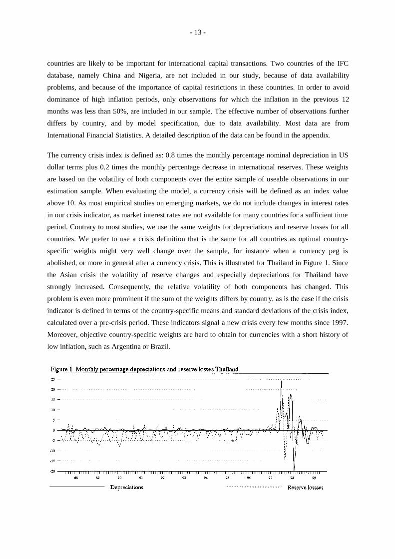
countries. We prefer to use a crisis definition that is the same for all countries as optimal country-

specific weights might very well change over the sample, for instance when a currency peg is

abolished, or more in general after a currency crisis. This is illustrated for Thailand in Figure 1. Since

the Asian crisis the volatility of reserve changes and especially depreciations for Thailand have

strongly increased. Consequently, the relative volatility of both components has changed. This

problem is even more prominent if the sum of the weights differs by country, as is the case if the crisis

indicator is defined in terms of the country-specific means and standard deviations of the crisis index,

calculated over a pre-crisis period. These indicators signal a new crisis every few months since 1997.

Moreover, objective country-specific weights are hard to obtain for currencies with a short history of

low inflation, such as Argentina or Brazil.

- 14 -

As explanatory variables, a wide range of variables is considered. In first instance all possible

candidates are included at the same time. Subsequently, variables that have the wrong sign, and

thereafter insignificant ones, are excluded. Regarding the time lag for explanatory variables, we

included at least a one-month lag for (real) exchange rates, international reserves, inflation rates, and

the currency regime, two months for GDP, exports, imports, M2, and bank credit, and five months for

international debt data. These relatively long time lags reflect the idea that economic variables become

especially important if market participants become aware of them. Also, in order to be useful as an

early warning indicator, long time lags are necessary.

5.2 Estimation results

Table 1 shows the estimation results for the model that was selected for the 1987-1996 period. Three

numbers are given for most parameters. The first is the value of the estimated coefficient. As the

model contains highly non-linear parts, this value is not always very informative. The second number

is a heteroskedasticity-consistent t-value. The last number, between square brackets, gives the average

change in the probability that the crisis indicator will exceed 10%, if the specific variable is changed

one standard deviation in the theoretically dangerous direction. This number gives some idea about the

economic relevance of the variables, although it should be noticed that no allowance is made for the

correlation between the explanatory variables. Moreover, it only gives the average change.

Economic variables do have a significant impact on the crisis index in various ways. In the linear part,

positive autocorrelation of reserve losses and depreciations are very prominent. Moreover, domestic

inflation and real overvaluation have a significant direct effect on the crisis index. This is in

accordance with the assumption that most countries allow their currency to depreciate gradually, if

necessary, in order to maintain competitive. Also for the variance, autocorrelation is very important.

As a matter of fact, a quite disturbing result is that the most important factors predicting a crisis, are

the recent developments in reserves and exchange rates themselves. Nevertheless, some other factors

matter as well. The influence on the variance of past local volatility, defined as the cross-sectional

variance computed over all other countries in the same continent, can be explained by the correlation

between exchange rate changes in neighbouring countries, combined with the clustering of volatility

over time. Free float currencies have a slightly higher volatility in normal times.

Domestic inflation, overvalued real exchange rates and reserve losses not only have a direct (linear)

effect on the crisis indicator, but also through the probability of entering the volatile regime. For the

probability of a crisis, defined as a crisis index of at least 10, this indirect effect dominates the direct

effect. Other variables that have a significant impact on the probability are the ratio of imports over

exports, the reserves over M2 ratio, and the annual growth rate in short-term debt over reserves.

Consequently, a crisis may be triggered by solvency problems (high imports over exports ratio, or an

overvalued currency), as well as liquidity related problems. Regarding liquidity, notice that over the

- 15 -

1987-1996 sample the reserves over M2 ratio is economically and statistically more important than the

short-term debt over reserves ratio. The latter variable is, however, very important for explaining the

depth of a crisis, as the additional variance in the crisis regime is completely dominated by this

variable. This result might explain why the influence of the M2 over reserves ratio is absent in

Bussière and Mulder (1999), as they only investigated the severity of crises. The additional expected

depreciation in the crisis regime is only limited. The only economic variable for which some influence

was found, is the average depreciation in neighbouring countries in the previous month. This variable

reflects contagion effects in currency markets. In the absence of local depreciations in the previous

month, the crisis indicator is only expected to grow by an additional 0.21 percentage point in the crisis

regime. The explanation for the limited size of this effect is probably that the timing of currency

depreciations, or reserve losses, is not well predictable, otherwise market participants could make huge

arbitrage profits. The influence on uncertainty is much more important.

Table 1: Estimation results for optimal specification over 1987-1996 Estimation sample 1987-1996 1987-1999 1997-1999

itX1 : linear expectation

Intercept -1.26 (2.7) -1.93 (4.2) -2.81 (2.7)Quarterly depreciation 0.112 (6.9) [0.22] 0.109 (7.6) [0.23] 0.069 (2.8) [0.32]Quarterly growth in reserves -0.011 (3.5) [0.12] -0.014 (4.5) [0.15] -0.019 (2.8) [0.18]Domestic annual inflation 0.015 (3.2) [0.06] 0.013 (3.0) [0.06] 0.019 (1.7) [0.09]Real exchange rate 0.22 (2.1) [0.02] 0.39 (3.8) [0.03] 0.63 (1.7) [0.08]

itX 2 : normal variance

Intercept 0.28 (3.2) 0.32 (3.2) 0.95 (2.3)Floating rates 0.51 (1.4) 0.04 (0.1) 0.00 (0.0)Exchange rate volatility (6 months weighted) 9.45 (4.5) [1.52] 11.70 (6.9) [2.22] 10.45 (5.0) [8.41]Reserves volatility (6 months weighted) 0.60 (3.9) [2.47] 0.58 (5.2) [2.37] 0.29 (1.9) [0.17]Average local exchange rate volatility (3mw) 1.17 (2.0) [0.02] 0.44 (0.9) [0.01] 0.00 (0.0) [0.00]

itX 3 : crisis regime probability

Intercept -9.00 (3.0) -6.57 (2.2) -1.19 (0.2)Real exchange rate 1.42 (2.1) [0.30] 0.99 (1.6) [0.26] 0.35 (0.2) [0.16]Domestic annual inflation 2.84 (2.2) [0.31] 2.07 (1.9) [0.28] 1.80 (0.6) [0.31]Imports over exports ratio 0.62 (3.0) [0.34] 0.25 (1.2) [0.17] -1.67 (2.4) [-1.03]Weighted quarterly growth in reserves -0.86 (2.0) [0.50] -0.82 (2.5) [0.62] -0.37 (0.8) [0.27]Annual growth short-term debt over reserves 0.43 (1.8) [0.24] 0.55 (2.5) [0.40] 1.61 (3.9) [1.74]Reserves over M2 ratio -3.50 (2.8) [0.70] -3.07 (3.0) [0.78] -4.41 (1.9) [1.71]

itX 4 : crisis regime additional expectationIntercept 0.21 (0.5) 0.78 (1.6) 2.55 (1.6)Local average monthly depreciation 0.38 (1.6) [0.18] 0.35 (1.5) [0.18] 0.31 (0.9) [0.38]

itX 5 : crisis regime additional variance

Intercept 0.00 (0.0) 0.00 (0.0) 3.33 (0.4)Short-term debt over reserves ratio 35.99 (2.1) [1.17] 46.82 (2.7) [1.19] 79.67 (1.6) [0.69]

Number of observations 2557 3312 755

Note: Heteroskedasticity consistent absolute t-values in parentheses. Between square brackets, the increase,

measured in percentage points, in the probability of obtaining a crisis indicator value of at least 10, due to a one

standard deviation change in the explanatory variable, evaluated over the 1987-1996 sample, is shown.

- 16 -

In order to investigate parameter stability, the same model that was selected for our 1987-1996

sample, was also estimated for our full sample (May 1987-June 1999), and for the most recent period

only (1997-1999). Unfortunately, not all parameters are stable. Partly, this might be explained by

multicollinearity. The most remarkable changes are related to the probability of entering the crisis

regime. The liquidity related variables have become much more important over the recent period,

whereas the influence of solvency related variables has declined. Especially the imports over exports

ratio changes dramatically, and even becomes significantly negative over the 1997-1999 period. Also,

the influence of the real exchange rate and inflation decline, but these effects are somewhat

compensated for by a higher direct effect of these variables. Regarding the liquidity variables, the

influence of the growth rate of short-term debt to reserves is very significant. The reserves over M2

ratio also remains significant however.

Somewhat surprising, the influence of contagion seems to have declined over the latter period. Where

the influence of local depreciations on the additional expected depreciation in the crisis regime has

hardly changed, the influence of past local volatility on the variance has declined. Given the

worldwide effects of the Asian and Russian crises, this result seems contra-intuitive. One reason for

this result might be that contagious effects materialise quicker, that is to say within one month, lately.

If that should be the case, contagion would not show up in the influence of past depreciations in

neighbouring countries, but in the depreciation of the own currency. Indeed the influence of own past

exchange rate volatility has increased. In order to investigate the possibility that contemporaneous

correlations have increased lately, covariance matrices of normalised residuals of our model were

calculated, based on a one year moving window.7 Only twelve countries are used for this purpose, as

data for the other countries was lacking, or excluded because of excessive inflation. Figure 2 shows

the cumulative explanatory power of the first three principal components based on these covariance

matrices. About 75% of the variance of those twelve crisis indicators can be explained by three

common factors. Although the explanatory power of the first three principal components has increased

somewhat in recent years, the current level is comparable to the levels of the early nineties. Therefore,

we do not find convincing evidence of increased contagion, other than can be explained by the

variables in our model, over recent years.

7 The normalised residuals are computed by means of the cumulative distribution function. For each residual the probability

of finding a smaller value than the one observed is calculated. Subsequently, the corresponding normalised residual is

computed by means of the inverse of the standard normal cumulative distribution function (Palm and Vlaar, 1997). This

normalisation procedure has the advantage that the influence of outliers is reduced.

- 17 -

5.3 Sensitivity analysis

Although the model shown in Table 1 gives a plausible representation of the data, it does not contain

many other variables that might be important. Table 2 gives a selected overview of alternative

specifications. The table only provides the t-values, with a negative sign indicating that the sign of that

variable was wrong. The variables from Table 1, except for the intercepts, are shown in Columns 2 to

17, whereas in Column 1 the t-value for the additional variable is shown.

We tried several alternative specifications for the level of the real exchange rate. Ideally, one should

include the deviation from an equilibrium value, but obviously this value is not available. We used the

logarithm of the real exchange rate, normalised at 100 in 1990. We prefer this procedure above one in

which the deviation from the mean or from a deterministic trend is used, because the latter procedures

incorporate information of all future exchange rates within sample, thereby generating spurious

results. Our procedure might have the same problem for the 1987-1990 part of the sample. Real

appreciations over a given period only use information that was available to the market, so they might

be preferred. However, we do not find empirical support for the influence of real appreciations. The

table includes the results for the four-year appreciation on the linear part, the crisis regime probability,

and on the expected extra depreciation in the crisis regime, but none of these is successful. Similar

results (not shown) were obtained for the one-year real appreciation or for the current two-year

average relative to the ten years before, as in J.P. Morgan (1998). A possible explanation might be that

our model includes the domestic inflation rate, which is highly correlated with the (annual) real

depreciation rate.

The influence of global contagion was investigated for the normal and crisis regime variance and for

the crisis regime mean. None of these effects was important. The variances were hardly affected, and

the influence on the crisis regime mean was negative if the average depreciation in the country’s own

continent was also included. Financial contagion was also investigated by means of changes in stock

market indices. If currency crises are indeed strongly related to market sentiment, as was concluded by

- 18 -

J.P. Morgan, developments on stock markets of emerging markets might signal future patterns in

exchange markets. We tried several specifications, both global and local, but for the 1987-1996

sample none was significant. For our full sample however, the quarterly change in stock market

indices averaged over all emerging markets included did have a significant impact on the probability

of entering the volatile regime.

Credit growth to the private sector is often used as an indicator of the healthiness of the banking

sector. Rapid credit growth is likely to be accompanied by more dubious loans, for instance due to a

bubble in the real estate sector. Kaminsky et al. (1998) conclude that most studies on currency crises

that include the growth in credit over GDP find significant impact of credit growth on the probability

of a currency crisis. However, we do not find any significant influence if the annual growth rate is

included, and a significant wrong sign if the four-year growth is considered. Possibly, the adverse

impact of credit growth documented by others is mainly due to foreign funding, which in our standard

model is already captured by the short-term debt variables.

The level of the short-term debt to reserves ratio was included in the crisis regime probability and

mean. In both specifications the sign turned out to be wrong. The exchange rate regime was included

in all five instances. Only for the variance in the quiet regime it had some significance.8 One would

expect the average size or volatility of a crisis to be higher for pegged currencies, but this could not be

detected. Real growth only has a small and insignificant impact on the probability of crisis. Also if

(expected) growth is approximated by the growth of the own stock market index, no influence is

detected. The influence of yearly export growth, as included in the EWS model of the IMF, as well as

the growth in the ratio of imports over exports turn out to have the wrong sign for the volatile regime

probability, though they are insignificantly different from zero.

Finally, the controversy whether solvency or liquidity problems are the most important cause for

currency crises is further investigated by including the (growth of) total debt at banks over exports

ratio. Surprisingly enough, both variables decrease the probability of entering the volatile regime.

Therefore, our results suggest that the stock of debt is not very important in explaining a currency

crisis, but increasing solvency problems related to real overvaluation, materialising in trade balance

deficits, are.

Regarding the t-values of the variables of the standard model, it is promising that these are hardly

affected by the inclusion of alternative variables. At least, the model is stable in that respect.

8 As variance parameters are restricted to be positive, a one-sided confidence interval is used. Consequently, the variable is

just significant at the 10% level.

- 19 -

Table 2: Alternative specifications for the 1987-1996 sample

X1 X2 X3 X4 X5

Alte

rnat

ive

vari

able

Dep

reci

atio

n

Res

erve

loss

es

Infl

atio

n

Rea

lex

chan

ge r

ate

Floa

ting

regi

me

Exc

hang

e ra

tevo

latil

ity

Res

erve

svo

latil

ity

Loc

alvo

latil

ity

Rea

lex

chan

ge r

ate

Infl

atio

n

Impo

rts

/ex

port

s

Gro

wth

rese

rves

Gro

wth

sho

rtde

bt /

rese

rves

Res

erve

s / M

2

Loc

alde

prec

iatio

n

Shor

t deb

t /re

serv

es

X1Real appreciation over 4 years -0.8 6.8 3.2 3.1 2.2 1.4 4.1 3.8 2.0 2.2 2.2 3.1 1.9 1.9 2.8 1.5 2.2

X2Global exchange rate volatility 0.6 6.9 3.4 3.1 2.1 1.4 4.5 3.9 2.0 2.2 2.2 3.0 1.9 1.8 2.8 1.6 2.1

X3Real appreciation over 4 years -1.2 6.8 3.2 3.1 2.2 1.5 4.3 3.7 2.0 2.3 2.2 3.2 1.9 2.0 2.8 1.5 2.2Annual growth credit / GDP 0.5 6.8 3.3 3.1 2.2 1.5 4.2 4.2 2.0 1.8 2.6 3.1 1.9 2.1 2.7 1.8 2.24 year growth credit / GDP -2.0 7.3 2.8 2.0 1.7 1.5 3.5 4.5 2.1 2.4 2.3 3.0 2.4 2.1 2.1 1.0 1.3Global quarterly stock index growth 0.6 6.9 3.5 3.2 2.1 1.4 4.4 3.9 2.0 2.2 2.2 3.0 1.9 1.8 2.8 1.6 2.1Short-term debt / reserves -1.3 6.9 3.4 3.3 2.0 1.4 4.5 4.1 2.0 1.8 2.4 2.3 2.0 2.0 3.0 1.6 2.2Managed or pegged regime 0.3 6.9 3.5 3.2 2.1 1.2 4.5 3.8 2.0 2.0 2.2 2.9 1.8 1.8 2.7 1.6 2.1Annual real GDP growth 0.8 6.8 3.3 3.1 2.2 1.4 4.1 4.1 2.0 2.0 1.8 3.0 2.1 2.0 2.7 1.3 2.2Annual growth imports / exports -0.7 6.7 3.0 3.5 1.4 1.4 4.0 3.9 2.0 2.0 2.2 3.1 2.0 1.8 2.7 1.6 2.1Yearly export growth -1.3 6.6 3.1 3.5 1.4 1.4 4.2 4.0 2.0 2.0 2.3 3.1 2.0 1.7 2.8 1.6 2.1Total debt (at banks) / exports -1.1 6.9 3.4 3.2 2.1 1.4 4.3 3.8 2.0 2.2 2.3 3.2 1.9 1.8 2.8 1.5 2.1Annual growth total debt / exports -0.8 6.6 3.0 3.5 1.4 1.4 4.3 4.0 2.0 1.9 1.9 3.1 1.9 1.9 2.7 1.6 2.1

X4Real appreciation over 4 years 0.8 6.9 3.2 3.1 2.1 1.4 4.2 4.0 2.0 2.1 2.2 3.0 2.0 1.9 2.8 1.5 2.2Managed or pegged regime -1.2 6.8 3.5 3.2 2.2 1.4 4.5 4.1 2.0 2.3 2.2 3.2 2.0 1.8 2.9 1.6 2.2Short-term debt / reserves -1.9 6.9 3.5 3.2 2.1 1.4 4.5 4.0 2.0 2.1 2.2 3.1 2.0 1.9 2.8 1.8 2.1Real exchange rate 1.5 6.9 3.5 3.2 1.8 1.4 4.5 4.1 2.0 2.0 2.1 2.8 2.0 1.9 2.8 1.8 2.2Average global depreciation -1.4 6.9 3.4 3.1 2.1 1.4 4.4 4.0 2.0 2.2 2.2 3.0 2.0 1.8 2.9 2.1 2.1

X5Managed or pegged regime 0.0 6.9 3.5 3.2 2.1 1.4 4.5 3.9 2.0 2.1 2.2 3.0 2.0 1.8 2.8 1.6 2.1Local exchange rate volatility 0.3 6.8 3.4 3.2 2.1 1.4 4.3 3.9 2.0 2.1 2.2 3.0 1.9 1.8 2.8 1.1 2.1Real exchange rate 0.0 6.9 3.5 3.2 2.1 1.4 4.5 3.9 2.0 2.1 2.2 3.0 2.0 1.8 2.8 1.6 2.1Global exchange rate volatility 0.0 6.9 3.5 3.2 2.1 1.4 4.5 3.9 2.0 2.1 2.2 3.0 2.0 1.8 2.8 1.6 2.1Note: Shown are the heteroskedasticity-consistent t-values. A negative sign indicates the theoretically wrong sign for that variable.

- 20 -

5.4 Crisis prediction

Despite the fact that the optimal model for 1987-1996 differs from the one over 1997-1999, it is

interesting to see to what extent the model that is estimated over 87-96 can be used to predict

exchange rate crises over the years thereafter. The fact that the model can be improved, does not

necessarily mean that the original formulation is useless with respect to forecasting. Especially if the

parameter instability is primarily due to multicollinearity, the model might still be successful in

forecasting. For that purpose, a currency crisis is defined as a value for the currency crisis indicator of

at least 10%. So defined, our sample contains 49 currency crises, 25 before 1997, and 24 thereafter.

The total number of crises over the sample for the 31 countries included in the study is somewhat

higher, but we only analyse crisis for which we have data on both the indicator and the explanatory

variables, and for which inflation over the previous twelve months was less than 50%.

Table 3 Predictive power crisis index modelAll observations Excluding 2 months after crisis

Crises Tranquil Noise/signal Crises Tranquil Noise/signal

Within sample: May 1987 - December 1996

Total 25 2532 21 2493p10% > 10% 10 111 0.110 6 77 0.108p10% > 5% 14 308 0.217 10 270 0.227p10% > 2% 21 608 0.286 17 569 0.282p10% > 1% 23 913 0.392 19 874 0.387

p10% > 0.5% 24 1315 0.541 20 1276 0.537p10% > 0.2% 25 1649 0.651 21 1610 0.646

Out-of sample: Januari 1997- June 1999

Total 24 731 16 704p10% > 10% 13 39 0.098 5 18 0.082p10% > 5% 14 73 0.171 6 49 0.186p10% > 2% 17 151 0.292 9 124 0.313p10% > 1% 21 227 0.355 13 200 0.350

p10% > 0.5% 23 345 0.492 15 318 0.482p10% > 0.2% 24 454 0.621 16 427 0.607

Note: The noise to signal ratio is defined as number of bad signals as a share of possible bad signals,divided by the number of good signals as a share of possible good signals.

Table 3 shows the predictive power of our model. The success to predict crises naturally depends on

the threshold used to select vulnerable observations. Within sample, if the threshold level is set at

10%, meaning that a warning signal is given whenever the probability of a crisis is at least 10%, 10

out of 25 crises are detected. This comes at the expense of also selecting 111 quiet periods out of

2532. This large number of tranquil periods selected should not come as a surprise, as our model

predicts that the probability of selecting a tranquil period is up to 90%. Indeed, one should not expect

to be able to select crisis observations without signalling tranquil periods as well, since this would lead

- 21 -

to arbitrage opportunities. If the threshold is lowered to 1%, 23 out of 25 crisis observations are

selected, but also about 37% of tranquil periods. At the 0.2% level all crises are selected. The higher

the threshold, the more selective is the model. This is reflected in the noise to signal ratio, which rises

from 11.0% to 65.1% when lowering the threshold from 10% to 0.2%.

Although the noise to signal ratio of our model seems good, one may wonder whether the model is

really informative, or simply providing information that is already known. More precisely, given the

importance of past depreciations and reserve losses in our model, part of the crises that we signal are

simply continuations of a crisis in the previous period. In order to detect the importance of these

repeated crises, we also calculated the predictive power for a restricted sample, where observations for

a country are excluded up to two months after a crisis in that country. These results are shown in the

right hand sight of Table 3. Within sample four crises were continuations of previous ones, and all

four are detected at the 10% threshold. However, as 34 out of 39 non-crisis observations that followed

a crisis were also signalled as a crisis at the 10% threshold, the noise to signal ratios are hardly

affected by the truncation.

Out of sample, the results are about as good as within sample. Most of the noise to signal ratios are

even slightly lower out of sample. Apparently, the fact that not all model parameters are stable over

the sample does not affect the predictive power very much. The number of repeated crises is much

higher in the forecast period. As in the estimation period, these are all predicted at the 10% threshold

level. All in all, the results seem reasonable. At the 1% threshold level 87.5% of crises are detected, at

the price of signalling 33% of the time.

In order to get a better idea which crises are predicted, Table 4 provides the complete list of crises

included in the study. The crises that are best predicted are of course those that immediately followed

other crises. Most of the major first crises are detected only at the 1% level. The probability of a crisis

in Thailand in July 1997 was only 1.3% and the one in Russia in August 1998 1.0%. The Mexico crisis

was predicted at the 4.7% level if December 1994 is taken as the crisis date. If the start of this crisis is

located at November, during which the crisis indicator was 5.9, the probability of a crisis was 1.4%.

The one big crisis that is missed at the 1% level is the recent one in Brazil, for which the probability

according to our model was only 0.8%. This is all the more surprising because this was probably the

best-anticipated crisis ever. One reason for the relative poor performance of the model for this crisis is

the fact that Brazil had increased its foreign reserves in December 1998 by 8.5%. Consequently, the

probability of crisis had sharply reduced. Another reason is that the real exchange rate was hardly

giving a sign of overvaluation, due to the fact that it was even slightly more overvalued during the

reference period (1990). This example clearly shows the theoretical advantage of including real

appreciation over a fixed period, instead of the level of the real exchange rate. However, as we have

shown, we could not find empirical support for that formulation.

- 22 -

Table 4 Characteristics of the currency crises in our sampleDate Country Crisis index Probability of crisis Lambda Annual Inflation8801 Jordan 11.4 3.07 13.4 -1.88802 Poland 14.6 5.13 24.6 46.78804 Jordan 14.7 22.62 82.3 1.78806 Jordan 15.0 32.05 86.1 0.38903 Venezuela 121.7 9.01 53.9 43.59010 Pakistan 13.3 4.59 27.5 10.69101 Ecuador 10.4 0.92 2.3 49.59103 Portugal 11.1 2.08 14.9 12.99103 Zimbabwe 12.5 2.71 6.7 18.89106 Zimbabwe 13.3 19.59 49.0 22.29107 India 13.6 17.24 65.3 13.09109 Zimbabwe 17.8 35.32 0.0 22.09205 Ecuador 11.0 2.69 15.6 49.69301 Zimbabwe 12.9 10.82 24.9 46.39303 India 11.1 0.33 11.5 5.79307 Pakistan 13.9 15.15 61.8 9.69309 Pakistan 11.5 20.50 3.4 9.89401 Zimbabwe 11.3 1.14 5.7 18.69405 Venezuela 35.7 1.38 18.7 48.19412 Mexico 53.7 4.69 30.6 6.99501 Mexico 11.4 42.21 78.0 7.19503 Mexico 18.9 40.38 4.3 14.39510 Mexico 11.7 3.11 10.6 43.59604 South Africa 14.9 8.14 28.2 6.39610 Pakistan 15.7 9.14 45.2 9.89707 Philippines 10.8 0.69 19.0 5.79707 Thailand 20.7 1.33 14.5 4.49708 Indonesia 14.4 1.53 8.3 5.49709 Zimbabwe 12.9 10.55 48.1 18.09710 Indonesia 11.6 16.63 6.3 7.39711 Korea 20.5 2.26 9.9 4.29711 Zimbabwe 19.7 12.51 38.4 16.09712 Indonesia 23.6 12.16 7.8 8.89712 Korea 39.8 20.85 14.8 4.39712 Philippines 15.0 5.82 15.8 7.59712 Thailand 13.5 11.93 9.6 7.69801 Indonesia 96.6 32.55 6.0 10.39801 Malaysia 14.9 10.89 7.9 2.99801 Thailand 13.2 21.55 6.4 7.69805 Indonesia 30.7 25.54 5.7 42.59806 Indonesia 33.5 34.73 2.5 49.79806 Pakistan 10.3 3.31 15.9 5.69806 South Africa 13.5 1.89 11.1 5.19808 Mexico 10.6 0.49 7.5 15.49808 Russia 29.5 1.01 7.9 5.69809 Ecuador 14.0 3.85 28.0 34.29809 Russia 81.0 30.36 38.6 9.59901 Brazil 55.2 0.82 9.1 1.79902 Ecuador 25.0 10.37 24.9 42.3

Note: Lambda represents the probability of entering the crisis regime of our model. The annual

inflation denotes the inflation rate over the twelve months before the crisis.

- 23 -

Apart from the probability of crisis, which incorporates all elements of our model, Table 4 also shows

the probability of entering the crisis regime (lambda). The main reason for showing both is that the

probability of crisis is dominated by current volatility, whereas lambda signals vulnerabilities due to

economic circumstances. Consequently, this crisis indicator might be better suited to signal first crises.

Once a currency is in crisis, lambda is likely to reduce as the real exchange rate, and possibly the trade

balance, improve. Despite this lower lambda the probability of crisis will remain high due to the

lagged volatility effect. The average value of lambda over the estimation sample turned out to be

12.7%. During most crises, lambda was much higher. However, even for some of the first crises, for

instance the one for Brazil in January 1999, it was lower than the average value. This is probably due

to country specific effects, for instance due to an overvalued real exchange rate in 1990, the relative

importance of trade for the current account, or differences in measurement.

In order to visualise country specific differences, and in order to be able to say something about the

lead-time of these indicators, Figure 3 shows both the probability of crisis and lambda for the

countries included in this study.9 As a predictive device the developments in lambda are probably

more informative than the probability of crisis itself. For most first crisis episodes, lambda has

increased in the years before the crisis, although for some crises lambda started increasing only a few

months before. Clear examples are Malaysia, Thailand, The Philippines, and to a lesser extent Korea

during the Asian crisis, Mexico before the 1994 crisis, Ecuador before 1998, and Venezuela before

1989 and 1994. The level of lambda is less informative, as there are clear differences between

countries. The probability of crisis indicator is clearly dominated by current volatility. Consequently,

this measure is not very useful to predict first crises. Even if this probability is almost zero, for

instance due to an extremely regulated currency, a crisis might erupt if the fundamentals are weak.

Once a crisis has erupted, the probability of further crises strongly increases, whereas lambda is

reduced. Viewed from these results, the predictive properties shown in Table 3 can probably be

improved if (changes in) lambdas are taken into account as well.

Finally, what does our model say about the next crisis? Viewed from the developments in lambda, the

clearest example of increased vulnerability is probably given for Egypt. Indeed, rumours about an

upcoming devaluation of the Egyptian pound are widespread. Furthermore, several Latin American

countries (Ecuador, Colombia, Peru, Venezuela, and possibly Argentina) are clearly vulnerable,

whereas the Asian countries seem to have stabilised.

9 Turkey is not included as the inflation rate of Turkey was only below 50% annually before 1988. Missing values for

economic variables included in the model were replaced with last known values in order to avoid discontinuous lines. The

probability of crisis and lambda are bounded above by 10% and 25% respectively.

- 24 -

- 25 -

- 26 -

- 27 -

6 CONCLUSIONS

In this paper, a new method is introduced to predict currency crises. The method models a monthly

continuous crisis index based on depreciations and reserve losses, using observations of both crisis

periods and quiet times. The fact that during currency crises, the behaviour of market participants

differs from normal circumstances is modelled by means of an econometric model with two regimes,

one for troubled, volatile times, and one for normal episodes. The model is capable of separating the

variables that influence the probability of a currency crisis, from those that have an impact on the

depth of a crisis. The probability of crisis is in our model directly related to the probability of entering

the volatile regime. Relevant variables turn out to be the real exchange rate, the inflation rate, the

growth of the short-term debt over reserves ratio, growth in reserves, the reserves over M2 ratio, and

the imports over exports ratio. Developments in these variables should be particularly monitored in

order to prevent future crises. Variables influencing the depth of a crisis have in our model a

significant impact on the extra expected depreciation and extra volatility in the crisis regime. Local

depreciations and the short-term debt over reserves ratio turn out to be the crucial variables here.

When comparing results for 1987-1996 with those for 1997-1999, several differences are noticeable.

The main difference between the two periods is that the short-term debt over reserves ratio has become

much more important lately, whereas the imports over exports ratio seems to have lost its explanatory

power. This indicates that recent crises were probably more liquidity driven than previous ones. No

clear evidence is found for increased contagion effects. The influence of local depreciations in

previous months seems to have declined somewhat, whereas the contemporaneous correlations of the

normalised residuals of our model only rose slightly. This result seems surprising given the worldwide

impact of the Asian crisis. However, the domino effects of this crisis, as well as the large impact on

the world economy might also be explained by the fact that these countries were much more open, and

more developed than most previous targets of currency attacks. Consequently, large initial

depreciations immediately affected the economic growth potential for neighbouring countries, as they

were competing to a large extent on the same markets, and relied on exports for their growth.

The model is reasonably successful in predicting currency crises, also out of sample. If the threshold

above which the model gives a warning signal for an upcoming crisis is set at one percent, 21 out of

24 crises are predicted out of sample. This comes at the price of also giving a warning signal 35% of

the time no crisis is upcoming however. The clearest signals are provided for crises that followed other

crises. First crises are better detected by changes in the probability of entering the crisis regime (the

lambda). These provide a good summary of changes in the economic vulnerability of currencies,

although in some instances a lambda only started increasing a few months before the crisis. As the link

between vulnerabilities and currency crises is far from perfect, one can not expect to detect all

currency crises with the help of just one econometric model however.

- 28 -

APPENDIX: DATA SOURCES

General: The countries included in this study are: Argentina, Brazil, Chile, Colombia, Czech republic,

Ecuador, Egypt, Greece, Hungary, India, Indonesia, Israel, Jordan, Korea, Malaysia, Mexico,

Morocco, Pakistan, Peru, Philippines, Poland, Portugal, Russia, Slovakia, South Africa, Sri Lanka,

Taiwan, Thailand, Turkey, Venezuela, and Zimbabwe. The database consists of monthly observations

for January 1970 to June 1999. Observations for countries with an annual inflation rate above 50% in

the previous month are excluded from the estimation and evaluation procedures. Most data come from

the August 1999 International Financial Statistics CD-ROM of the IMF. Additional data are from

Datastream or taken from the Internet. For Taiwan, which is not an IMF member, most data come

from the Directorate General of Budgeting and Accounting Statistics (DGBAS). All explanatory

variables are lagged at least one month and more if the publication lag of the data is likely to be

longer. In order to limit the influence of large reserve changes or nominal exchange rates, explanatory

variables involving these two variables are bounded to their mean plus or minus five standard

deviations. Local variables are calculated over usable observations of the included countries per

continent (Asia, Latin America, Europe, or Africa plus the Middle East), excluding the country

concerned. Global variables are calculated over the usable observations of all included countries, again

excluding the country concerned. Whenever a weighted average of variable X over i months is used, it

is calculated as:

∑∑ =

−

= −−= i

j

i

j jtWi jXjiX1

1

0/)( .

Exchange rates: line ae of the IFS, end of period local currency per US dollar, except for Taiwan

(London exchange market). As explanatory variable, the variable is lagged in our model at least one

month.

International reserves: line 1..ld of the IFS, international reserves excluding gold in millions of US

dollars, except for South Africa for which total reserves including gold (line 1..sf) is used. For Taiwan

official reserves in US dollars, provided by DGBAS. As explanatory variable, the variable is lagged in

our model at least one month.

Currency crisis index: 0.8 * monthly percentage depreciation + 0.2 * monthly percentage reserve

losses. In the estimation process, this variable is bounded by 50%, in order to limit the influence of an

extreme observation (Venezuela, March 1989).

Consumer Price Index: line 64 of IFS. For Taiwan, the urban CPI provided by DGBAS is used. As

explanatory variable, the variable is lagged in our model at least one month.

Real exchange rates: CPI based trade weighted real exchange rates. Three different sources are used:

the measure of J.P. Morgan for Argentina, Brazil, Chile, Colombia, Ecuador, Greece, India, Indonesia,

- 29 -

Korea, Malaysia, Mexico, Morocco, Pakistan, Peru, Philippines, South Africa, Taiwan, Thailand,

Turkey, and Venezuela, the IFS measure (line rece) for Hungary, Israel, Poland, Portugal, Russia, and

Slovakia, and own calculations based on trade weights with Japan, the European Union and the US for

the Czech republic, Egypt, Jordan, Sri Lanka, and Zimbabwe. For our own calculations, period

average US dollar exchange rates (line af of IFS) and CPIs of Japan, Germany, the US and the

countries concerned are used. The trade weights are from various issues of the Direction of Trade

Statistics. As explanatory variable, the variable is lagged in our model at least one month.

M2: Sum of lines 34 and 35 of IFS. For Hungary, monthly observations provided by the National

Bank of Hungary are used. For Taiwan monthly figures are from DGBAS. As explanatory variable,

the variable is lagged in our model at least two months.

Credit: line 32d of IFS, domestic credit to private sector. For Taiwan, domestic credit to private sector

collected by DGBAS, and for Hungary, monthly consumer credit from the National Bank of Hungary.

As explanatory variable, the variable is lagged in our model at least two months.

Short-term foreign debt, and total foreign debt: BIS database. Bi-annual reports of foreign lending of

BIS reporting banks by country and remaining maturity. Short-term is defined as debt with a

remaining maturity of less than one year. As explanatory variables, these variables are lagged in our

model at least five months as there is a five-month publication lag. This means using the end of

December positions for the months May to October the next year, and the end of June positions for the

months November to April.

Exports and imports: line 70..d and 71..d of IFS, Exports and imports in millions of US dollars. As

explanatory variables, the variables are lagged in our model at least two months.

Gross Domestic Product: line 99b, GDP in current prices. This quarterly series is transformed to a

monthly series, using CPI and industrial production (line 66 of IFS) as indicators. The quarterly GDP

series for Taiwan is from DGBAS. If the IFS database did not provide monthly industrial production

series, other sources were used as well. The alternative sources for industrial production are: OECD

for Hungary, Poland, Portugal and Russia, Macroeconomica (Argentina), Lopes Filho & Associates

(Brazil), National statistical service of Greece, Biro Pusat Statistik (Indonesia), Statistics South Africa,

DGBAS (Taiwan), Bank of Thailand, State institute of statistics (Turkey), and Veneconomia

(Venezuela). As explanatory variable, the variable is lagged in our model at least two months.

Exchange rate regime: Annual report on exchange arrangements and exchange restrictions, IMF,

various issues.

- 30 -

BIBLIOGAPHY

Berg, A. and C. Pattillo (1998), ‘Are Currency Crises Predictable? A Test’, IMF Working Paper98/154.

Borenzstein, E., A. Berg, G.-M. Millesi-Ferretti and C. Pattillo (1999), ‘Anticipating Balance ofPayments Crises--The Role of Early Warning Systems’, IMF Occasional Paper, forthcoming.

Bussière, M. and C. Mulder (1999), ‘External Vulnerability in Emerging Market Economies: HowHigh Liquidity Can Offset Weak Fundamentals and the Effects of Contagion’, IMF Working Paper99/88.

Calvo, G. (1998), ‘Varieties of Capital-Market Crises’, in: Calvo, G. and M. King (eds.) The debtburden and its consequences for monetary policy, IEA Conference Volume, no. 118. New York: St.Martin's Press; London: Macmillan Press; in association with the International Economic Association.

Chang, R. and A. Velasco (1998), ‘Financial Fragility and the Exchange Rate Regime’, NBERWorking Paper 6469.

Frankel, J.A. and A.K. Rose (1996), ‘Currency Crashes in Emerging Markets: An EmpiricalTreatement’, Journal of International Economics 41, 351-66.

Glick, R. and A.K. Rose (1998), ‘Contagion and Trade: Why are Currency Crises Regional?’, NBERWorking Paper 6806.

Kaminsky, G.L., S. Lizondo and C.M. Reinhart (1998), ‘Leading Indicators of Currency Crises’,IMF Staff Papers 45, 1-48.

Kaminsky, G.L. and C.M. Reinhart (1996), ‘The Twin Crises: The Causes of Banking and Balance-of-Payments Problems’, International Finance Discussion Papers 544, Board of Governors of theFederal Reserve System.

Krugman, P. (1979), ‘A Model of Balance-of-Payments Crises’, Journal of Money, Credit andBanking 11, 311-25.

J.P. Morgan (1998), ‘Event Risk Indicator Handbook’, J.P. Morgan, London (can be downloadedfrom: WWW.jpmorgan.com).

Morris, S. and H.S. Shin. (1998), ‘Unique Equilibrium in a Model of Self-Fulfilling CurrencyAttacks’, American Economic Review 88, 587-597.

Obstfeld, M. (1986), ‘Rational and Self-Fulfilling Balance-of-Payments Crises’, American EconomicReview 76, 72-80.

Obstfeld, M. (1995), ‘The Logic of Currency Crises’, in: Eichengreen, B., J. Frieden and J. vonHagen (eds.) Monetary and fiscal policy in an integrated Europe. European and Transatlantic Studies,Heidelberg; New York and London: Springer, pages 62-90.

Palm, F.C. and P.J.G. Vlaar (1997), ‘Simple Diagnostic Procedures for Modelling Financial TimeSeries’, Allgemeines Statistisches Archiv 81, 85-101.

Sachs, J.D., A. Tornell and A. Velasco (1996), ‘Financial Crises in Emerging Markets: The Lessonsfrom 1995’, Brookings Papers on Economic Activity, 147-198.

- 31 -

Tornell, A. (1999), ‘Common Fundamentals in the Tequila and Asian Crises’, NBER Working Paper7139.

Velasco, A. (1987) ‘Financial Crises and Balance–of-Payments Crises’, Journal of DevelopmentEconomics 27, 263-283.

Vlaar, P.J.G. (1998), ‘Target Zones and Realignment Risk: An Integrated Approach’, De Economist146, 91-116.