
CuriousConvergencePropertiesofLatticeBoltzmann … · [email protected] (M.-M....
16
Commun. Comput. Phys. doi: 10.4208/cicp.OA-2016-0257 Vol. 23, No. 4, pp. 1263-1278 April 2018 Curious Convergence Properties of Lattice Boltzmann Schemes for Diffusion with Acoustic Scaling Bruce M. Boghosian 1 , François Dubois 2,3, ∗ , Benjamin Graille 2 , Pierre Lallemand 4 and Mohamed-Mahdi Tekitek 5 1 Department of Mathematics, Tufts University, Bromfield-Pearson Hall, Medford, MA 02155, USA. 2 Department of Mathematics, University Paris-Sud, Bât. 425, F-91405 Orsay, France. 3 Conservatoire National des Arts et Métiers, LMSSC laboratory, F-75003 Paris, France. 4 Beijing Computational Science Research Center, Haidian District, Beijing 100094, China. 5 Department of Mathematics, Faculty of Sciences of Tunis, University Tunis El Manar, Tunis, Tunisia. Received 16 December 2016; Accepted (in revised version) 22 April 2017 Abstract. We consider the D1Q3 lattice Boltzmann scheme with an acoustic scale for the simulation of diffusive processes. When the mesh is refined while holding the dif- fusivity constant, we first obtain asymptotic convergence. When the mesh size tends to zero, however, this convergence breaks down in a curious fashion, and we observe qualitative discrepancies from analytical solutions of the heat equation. In this work, a new asymptotic analysis is derived to explain this phenomenon using the Taylor ex- pansion method, and a partial differential equation of acoustic type is obtained in the asymptotic limit. We show that the error between the D1Q3 numerical solution and a finite-difference approximation of this acoustic-type partial differential equation tends to zero in the asymptotic limit. In addition, a wave vector analysis of this asymptotic regime demonstrates that the dispersion equation has nontrivial complex eigenvalues, a sign of underlying propagation phenomena, and a portent of the unusual conver- gence properties mentioned above. PACS: 02.70.Ns, 05.20.Dd, 47.10.+g Key words: Artificial compressibility method, Taylor expansion method. ∗ Corresponding author. Email addresses: (F. Dubois), (B. M. Boghosian), (B. Graille), (P. Lallemand), (M.-M. Tekitek) http://www.global-sci.com/ 1263 c 2018 Global-Science Press
Transcript of CuriousConvergencePropertiesofLatticeBoltzmann … · [email protected] (M.-M....

Commun. Comput. Phys.doi: 10.4208/cicp.OA-2016-0257
Vol. 23, No. 4, pp. 1263-1278April 2018
Curious Convergence Properties of Lattice Boltzmann
Schemes for Diffusion with Acoustic Scaling
Bruce M. Boghosian1, François Dubois2,3,∗, Benjamin Graille2,Pierre Lallemand4 and Mohamed-Mahdi Tekitek5
1 Department of Mathematics, Tufts University, Bromfield-Pearson Hall, Medford,MA 02155, USA.2 Department of Mathematics, University Paris-Sud, Bât. 425, F-91405 Orsay, France.3 Conservatoire National des Arts et Métiers, LMSSC laboratory, F-75003 Paris,France.4 Beijing Computational Science Research Center, Haidian District, Beijing 100094,China.5 Department of Mathematics, Faculty of Sciences of Tunis, University Tunis ElManar, Tunis, Tunisia.
Received 16 December 2016; Accepted (in revised version) 22 April 2017
Abstract. We consider the D1Q3 lattice Boltzmann scheme with an acoustic scale forthe simulation of diffusive processes. When the mesh is refined while holding the dif-fusivity constant, we first obtain asymptotic convergence. When the mesh size tendsto zero, however, this convergence breaks down in a curious fashion, and we observequalitative discrepancies from analytical solutions of the heat equation. In this work,a new asymptotic analysis is derived to explain this phenomenon using the Taylor ex-pansion method, and a partial differential equation of acoustic type is obtained in theasymptotic limit. We show that the error between the D1Q3 numerical solution and afinite-difference approximation of this acoustic-type partial differential equation tendsto zero in the asymptotic limit. In addition, a wave vector analysis of this asymptoticregime demonstrates that the dispersion equation has nontrivial complex eigenvalues,a sign of underlying propagation phenomena, and a portent of the unusual conver-gence properties mentioned above.
PACS: 02.70.Ns, 05.20.Dd, 47.10.+g
Key words: Artificial compressibility method, Taylor expansion method.
∗Corresponding author. Email addresses: fran ois.dubois�math.u-psud.fr (F. Dubois),bru e.boghosian�tufts.edu (B. M. Boghosian), benjamin.graille�math.u-psud.fr (B. Graille),pierre.lallemand1�free.fr (P. Lallemand), mohamedmahdi.tekitek�fst.rnu.tn (M.-M. Tekitek)
http://www.global-sci.com/ 1263 c©2018 Global-Science Press
1264 B. M. Boghosian et al. / Commun. Comput. Phys., 23 (2018), pp. 1263-1278
1 Introduction
Lattice Boltzmann models are simplifications of the continuum Boltzmann equation ob-tained by discretizing in both physical space and velocity space. The discrete velocitiesvi retained typically correspond to lattice vectors of the discrete spatial lattice. That is,each lattice vertex x is linked to a finite number of neighboring vertices by lattice vectorsvi∆t. A particle distribution f is therefore parametrized by its components in each of thediscrete velocities, the vertex x of the spatial lattice, and the discrete time t. A time stepof a classical lattice Boltzmann scheme [11] then contains two steps:
(i) a relaxation step where distribution f at each vertex x is locally modified into anew distribution f ∗, and
(ii) an advection step based on the method of characteristics as an exact time-integration operator. We employ the multiple-relaxation-time approach introduced byd’Humières [10], wherein the local mapping f 7−→ f ∗ is described by a nonlinear diago-nal operator in a space of moments, as detailed in Section 2.
In [5], we have studied the asymptotic expansion of various lattice Boltzmannschemes with multiple-relaxation times for different applications. We used the so-calledacoustic scaling, in which the ratio λ≡∆x/∆t is kept fixed. In this manner, we demon-strated the possibility of approximating diffusion processes described by the heat equa-tion.
In his very complete work, Dellacherie [3] has described unexpected results in sim-ulations for advection-diffusion processes. In this contribution, we endeavor to explainthose results by studying the convergence of the D1Q3 lattice Boltzmann scheme whenwe try to approximate a pure diffusion process.
We begin this paper by recalling some fundamental algorithmic aspects of the D1Q3lattice Boltzmann scheme in Section 2. Then, in Section 3 we describe a first illustrativenumerical experiment. In Section 4 we present a new convergence analysis, followed byanother numerical experiment in Section 5, in which the D1Q3 lattice Boltzmann schemeis studied far from the usual values of its parameters. Finally, a wave vector analysis isproposed in Section 6.
2 Diffusive D1Q3 lattice Boltzmann scheme
In this work, we consider the so-called D1Q3 lattice Boltzmann scheme in one spatialdimension. The spatial step ∆x > 0 is given, and each node x is an integer multiple ofthis spatial step : x∈Z∆x. The time step ∆t>0 is likewise given, and each discrete timet is an integer multiple of ∆t. We adopt so-called acoustic scaling (see e.g., [12]), so thenumerical velocity associated with the mesh,
λ≡ ∆x
∆t(2.1)

B. M. Boghosian et al. / Commun. Comput. Phys., 23 (2018), pp. 1263-1278 1265
is a constant independent of the spatial step ∆x. A particle distribution
f ≡(
f+(x,t) f0(x,t) f−(x,t))
is given at the initial step t = 0. Its value at subsequent times is determined by themultiple-relaxation-time version [10] of the lattice Boltzmann equation.
Moments are introduced at each step of space and time according to the relations
ρ= f++ f0+ f−, J=λ( f+− f−), e=λ2( f+−2 f0+ f−). (2.2)
These may be thought of as the densities of mass, momentum, and an energy-like quan-tity, respectively. Eq. (2.2) can be recast in matrix form as follows:
m≡
ρJe
=M f ≡M
f+f0
f−
,
where M is the invertible matrix,
M=
1 1 1λ 0 −λλ2 −2λ2 λ2
. (2.3)
The equilibrium values of the moments are defined by the relations:
ρeq=ρ, Jeq=0, eeq=αλ2
2ρ, (2.4)
where α a non-dimensional constant. Then the relaxation step transforms the pre-collision moments m into new post-collision moments m∗ as follows:
ρ∗=ρ, J∗= J+sJ(Jeq− J), e∗= e+se(eeq−e), (2.5)
where sJ and se are relaxation parameters. There is no analogous parameter for ρ becausethe collisions are constrained to conserve mass. In our numerical experiments, we havechosen se = 1.5, and below we shall explain in some detail how we tuned the relaxationparameter sJ for the momentum J.
The time iteration of the scheme is defined in terms of the particle distribution. Wefirst transform the post-collision moments m∗ into a post-collision particle distribution:
f ∗=M−1m∗.
Second, we iterate the algorithm forward in time. The particle distribution is conservedalong the characteristic directions of velocities v+=λ, v0=0 and v−=−λ respectively:
f+(x,t+∆t)= f ∗+(x−∆x,t),
f0(x,t+∆t)= f ∗0 (x,t),
f−(x,t+∆t)= f ∗−(x+∆x,t).
(2.6)
1266 B. M. Boghosian et al. / Commun. Comput. Phys., 23 (2018), pp. 1263-1278
In [5], we have analyzed several lattice Boltzmann models with the Taylor expansionmethod, including the present one defined by Eqs. (2.2), (2.3), (2.4), (2.5), (2.6). The hy-pothesis used was that the numerical velocity λ defined in Eq. (2.1), and the relaxationcoefficients sJ and se remain constant as the spatial step ∆x tends to zero. Then the con-served variable ρ satisfies (at least formally!) a diffusion partial differential equation:
∂ρ
∂t−µ
∂2ρ
∂x2=O(∆x2), (2.7)
where the diffusion coefficient µ is given by the relation
µ≡ 4+α
6σλ∆x, σ≡
( 1
sJ− 1
2
)
. (2.8)
The coefficient σ is known as the "Hénon parameter" in reference to the pioneering workof Hénon [9]. This lattice Boltzmann scheme is demonstrably stable under the condition:
−4<α<2.
3 A first numerical experiment
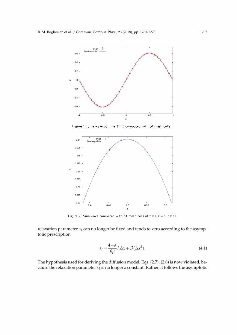
In this section, we consider an elementary analytic test case, namely the diffusion of asine wave. We suppose that the initial condition for Eq. (2.7) satisfies
ρ0(x)=sin(π x), −1≤ x≤1. (3.1)
The other moments J and e are taken at equilibrium at t = 0. With periodic boundaryconditions, the exact solution of Eqs. (2.7), (3.1) is
ρ(x,t)=sin(πx)exp(−µπ2t).
We performed several numerical computations with the following choice of parameters:λ= 1, α= 1 and µ= 0.01. The spatial step varied from ∆x= 1
4 up to ∆x= 132 . The results
for a final time T=5 are presented in Figs. 1 through 3.It should be noted that the results are remarkably converged even for these relatively
coarse meshes. For the most refined mesh used (64 mesh points, ∆x= 132 ), the numerical
results are almost indistinguishable from the exact solution, as presented in two succes-sive magnifications in Fig. 2.
4 An alternative convergence analysis
We now imagine that we wish to approximate the diffusion equation, Eq. (2.7), usingthe D1Q3 lattice Boltzmann model described previously. We suppose that the diffusioncoefficient µ is fixed and that the mesh size ∆x tends to zero. Then from Eq. (2.8), the
B. M. Boghosian et al. / Commun. Comput. Phys., 23 (2018), pp. 1263-1278 1267
Figure 1: Sine wave at time T=5 omputed with 64 mesh ells.
Figure 2: Sine wave omputed with 64 mesh ells at time T=5; detail.
relaxation parameter sJ can no longer be fixed and tends to zero according to the asymp-totic prescription
sJ =4+α
6µλ∆x+O(∆x2). (4.1)
The hypothesis used for deriving the diffusion model, Eqs. (2.7), (2.8) is now violated, be-cause the relaxation parameter sJ is no longer a constant. Rather, it follows the asymptotic
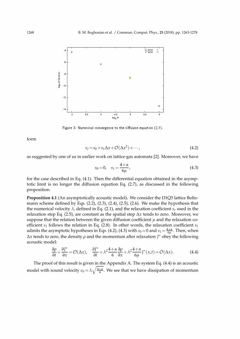
1268 B. M. Boghosian et al. / Commun. Comput. Phys., 23 (2018), pp. 1263-1278
Figure 3: Numeri al onvergen e to the di�usion equation (2.7).
form
sJ = s0+s1∆x+O(∆x2)+··· , (4.2)
as suggested by one of us in earlier work on lattice-gas automata [2]. Moreover, we have
s0=0, s1=4+α
6µ, (4.3)
for the case described in Eq. (4.1). Then the differential equation obtained in the asymp-totic limit is no longer the diffusion equation Eq. (2.7), as discussed in the followingproposition.
Proposition 4.1 (An asymptotically acoustic model). We consider the D1Q3 lattice Boltz-mann scheme defined by Eqs. (2.2), (2.3), (2.4), (2.5), (2.6). We make the hypothesis thatthe numerical velocity λ, defined in Eq. (2.1), and the relaxation coefficient se used in therelaxation step Eq. (2.5), are constant as the spatial step ∆x tends to zero. Moreover, wesuppose that the relation between the given diffusion coefficient µ and the relaxation co-efficient sJ follows the relation in Eq. (2.8). In other words, the relaxation coefficient sJ
admits the asymptotic hypotheses in Eqs. (4.2), (4.3) with s0=0 and s1=4+α6µ . Then, when
∆x tends to zero, the density ρ and the momentum after relaxation J∗ obey the followingacoustic model:
∂ρ
∂t+
∂J∗
∂x=O(∆x),
∂J∗
∂t+λ2 4+α
6
∂ρ
∂x+λ2 4+α
6µJ∗(x,t)=O(∆x). (4.4)
The proof of this result is given in the Appendix A. The system Eq. (4.4) is an acoustic
model with sound velocity c0 =λ√
4+α6 . We see that we have dissipation of momentum

B. M. Boghosian et al. / Commun. Comput. Phys., 23 (2018), pp. 1263-1278 1269
with a zero-order operator. We have implemented a staggered finite-difference methodnamed "HaWAY", in reference to the authors Harlow and Welch [8], Arakawa [1] andYee [13] who invented it in the mid 1960’s, for applications to fluid flow ("marker andcell"), geophysical sciences ("c-grid") and electromagnetism ("finite difference time do-main"), respectively. The details of this second-order numerical scheme are given in Ap-pendix B. This finite-difference approximation gives a correct second-order accurate so-lution of the system obtained by replacing the corrections O(∆x) by 0 on the right-handside of Eqs. (4.4).
5 Additional numerical experiments
We next experiment with the diffusion of a Gaussian density profile with the D1Q3 latticeBoltzmann model defined in this work. The initial density profile is given by the relation
ρ0(x)=exp(
− x2
4µ
)
with x∈R. (5.1)
The other moments J and e are taken to be at equilibrium at t=0. Then the exact solutionof the diffusion equation, Eq. (2.7), is obtained without difficulty:
ρ(x,t)=1√1+t
exp(
− x2
4µ(1+t)
)
, x∈R, t>0. (5.2)
We simulate this problem for µ=0.01 and 0≤t≤T=5 in a relatively large domain −16≤x≤16 in order to avoid unwanted interactions of the diffusing Gaussian with the boundary.This has allowed us to employ an elementary periodic boundary condition at x =±16,where all the fields have a value inferior to the smallest number that can be representedin floating-point arithmetic.
At the macroscopic scale, we see in Fig. 4 that the numerical solution computed withthe D1Q3 lattice Boltzmann scheme faithfully reproduces the exact solution Eq. (5.2) ofthe diffusion equation. After magnification by a factor of 100 (Fig. 5), the D1Q3 modelsimulates the acoustic-like system, Eq. (4.4), with better accuracy than it does the dif-fusion equation, Eq. (2.7). Fig. 6 shows that when the mesh is refined from 26 = 64 to216=65536 vertices, the convergence towards the acoustic model seems reasonable, withan order of accuracy close to 1. In other terms, the difference between the discrete solu-tion of the D1Q3 model and the finite-difference simulation of the acoustic model goes tozero proportionally to the mesh size.
Now we have what seems like a contradiction: Our first experiments for the sinewave show (see, e.g., Fig. 3) that the diffusion equation is a good reference mathematicalmodel, whereas the acoustic model Eq. (4.4) is asymptotically correct for the Gaussianinitial condition (see Fig. 6). We have performed simulations for the sine wave with muchmore refined meshes, and lattice sizes up to 4096. At the macroscopic scale, no differenceis visible between the sine wave solution of the diffusion equation and the numerical

1270 B. M. Boghosian et al. / Commun. Comput. Phys., 23 (2018), pp. 1263-1278
Figure 4: Gaussian a time T=5.
Figure 5: Detail of the Gaussian a time T=5.
result proposed by the lattice Boltzmann method (again, see Fig. 1). After magnificationshown in Fig. 7, the difference between the exact solution of the diffusion equation andthe D1Q3 solution is more important than the small discrepancy between the "HaWAY"numerical solution of the acoustic model, Eq. (4.4), and the lattice Boltzmann model.
In Fig. 8, we have plotted the quadratic and uniform errors between the numerical so-lution obtained from the lattice Boltzmann model and the exact solution of the diffusionequation on one hand, and of the approximate solution (with a second-order scheme)of the acoustic model obtained after a first-order Taylor expansion analysis presented at

B. M. Boghosian et al. / Commun. Comput. Phys., 23 (2018), pp. 1263-1278 1271
Figure 6: D1Q3 latti e Boltzmann s heme for di�usion; Gaussian at time = 5. Non- onvergen e towards the
exa t solution of the di�usion model Eq. (2.7) and onvergen e towards the a ousti model Eq. (4.4).
Figure 7: Sine wave at time =5. Magni� ation of the solution around the extremal value.
Proposition 1 on the other hand. The lattice Boltzmann method gives an excellent ap-proximation of the heat equation with the coarse meshes, as shown in Fig. 3 in Section 2.This good convergence quality cannot be explained by an asymptotic analysis. When thespatial step tends to zero, the lattice Boltzmann scheme gives a correct approximation ofthe acoustic model. Fig. 8 demonstrates that the convergence is first-order accurate inboth norms.

1272 B. M. Boghosian et al. / Commun. Comput. Phys., 23 (2018), pp. 1263-1278
Figure 8: D1Q3 latti e Boltzmann s heme for di�usion; Sine wave at time =5. Non- onvergen e towards the
exa t solution of the di�usion model Eq. (2.7) and onvergen e towards the a ousti model Eq. (4.4).
6 Wave vectors analysis
We may also adopt the point of view of a spectral analysis of the lattice Boltzmann model,Eqs. (2.2), (2.3), (2.4), (2.5), (2.6). We search for a solution of the type
f (x,t)=exp(
ikx)
exp(
ζt)
ϕ+
ϕ0
ϕ−
. (6.1)
In one time step, we first transform the vector f into moments. Then we relax the mo-ments and return to the space of particles. Finally we advect the result according toEq. (2.6) to recover the particle distribution. The collision step m−→m∗ can be written inmatrix form:
m∗=Rm, R=
1 0 00 1−sJ 0
α λ2
2 se 0 1−se
,
and the final advection step can be represented by the action of a diagonal matrix:
f (x,t+∆t)=A f ∗(x,t), A=
exp(−iξ) 0 00 1 00 0 exp(iξ)
,
B. M. Boghosian et al. / Commun. Comput. Phys., 23 (2018), pp. 1263-1278 1273
with ξ = k∆x. Then the vector ϕ introduced in Eq. (6.1) must be a nontrivial solution ofthe following spectral problem:
exp(
ζ)
ϕ=AM−1RMϕ,
with ζ=z∆t>0. Then, denoting the identity matrix by I, the dispersion relation takes theform
det[
AM−1RM−exp(
ζ)
I]
=0. (6.2)
We have performed an asymptotic analysis of the relation in Eq. (6.2) in the limit ofa small relaxation coefficient sJ (as in Eq. (4.1)), a small wave vector ξ and with a smallamplification factor ζ:
sJ = εs1, ξ= εκ, ζ= εω, (6.3)
where ε is a small parameter that tends to zero. After some calculation, we obtain withoutdifficulty
det[
AM−1RM−exp(
ζ)
I]
=−se
(
ω2+s1ω+4+α
6κ)
ε2+O(ε3). (6.4)
When κ = 0, we recover the hydrodynamic mode with ω = 0 and a dissipative modeaccording to ω=−s1. When κ 6=0, we have to solve an equation of degree 2 made explicitin Eq. (6.4) at this order of accuracy. The discriminant of this equation becomes negativewhen
κ≥ s1
2√
4+α6
. (6.5)
We observe that the asymptotics associated with the limit sJ−→0 is questionable froma physical point of view. When establishing macroscopic partial differential equations itis assumed that internal degrees of freedom of the system under study evolve very fastcompared to the macroscopic quantities. It is known (see, e.g., [4]) that sJ is given bya ratio of the type ∆t
τ . In the present case, the slow internal degrees of freedom evolve
within times τ ≈ ∆ts . So it is to be expected that the pure diffusion partial differential
equation will not be accurate for very small values of s.In order to make this qualitative difference explicit, we have done two numerical
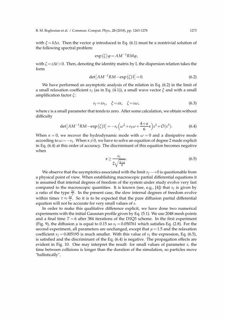
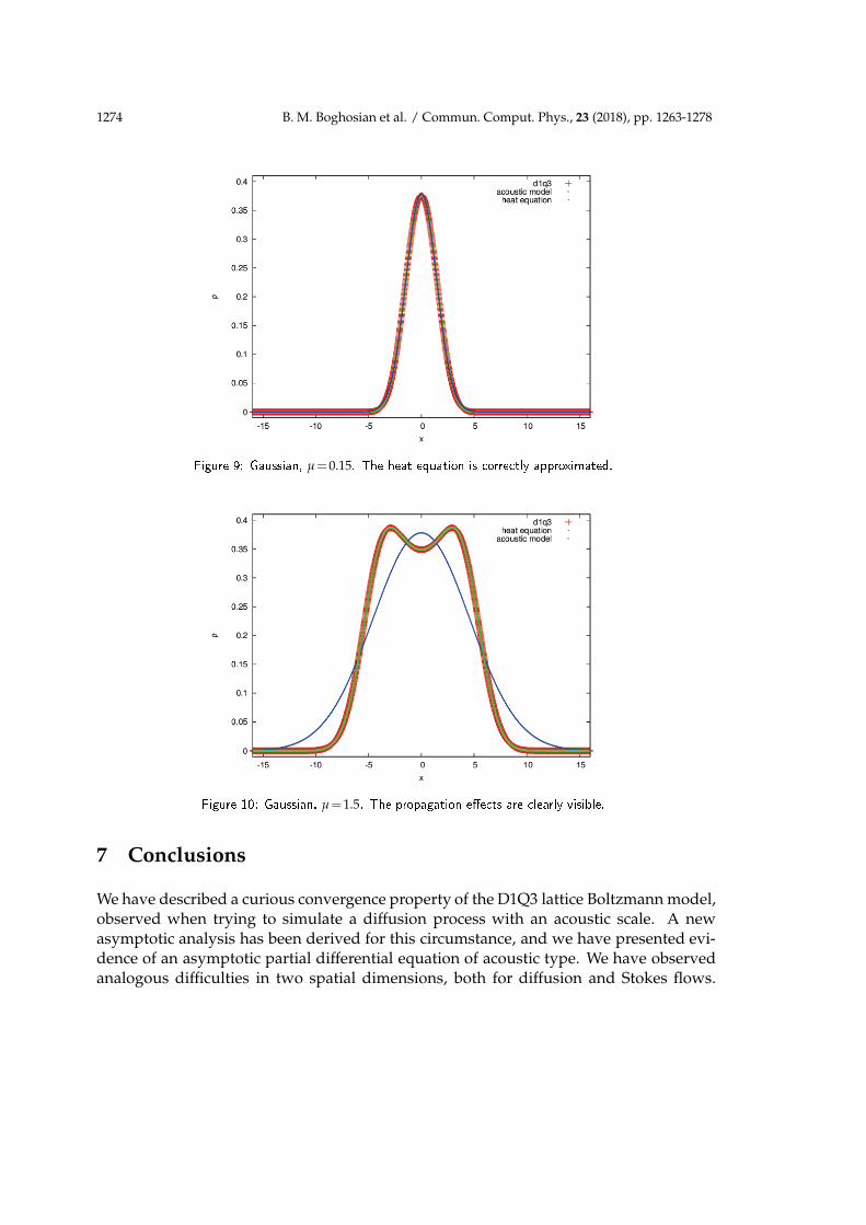
experiments with the initial Gaussian profile given by Eq. (5.1). We use 2048 mesh pointsand a final time T = 6 after 384 iterations of the D1Q3 scheme. In the first experiment(Fig. 9), the diffusion µ is equal to 0.15 so sJ = 0.050761 which satisfies Eq. (2.8). For thesecond experiment, all parameters are unchanged, except that µ=1.5 and the relaxationcoefficient sJ = 0.005195 is much smaller. With this value of sJ the expression, Eq. (6.5),is satisfied and the discriminant of the Eq. (6.4) is negative. The propagation effects areevident in Fig. 10. One may interpret the result: for small values of parameter s, thetime between collisions is longer than the duration of the simulation, so particles move"ballistically".
1274 B. M. Boghosian et al. / Commun. Comput. Phys., 23 (2018), pp. 1263-1278
Figure 9: Gaussian, µ=0.15. The heat equation is orre tly approximated.
Figure 10: Gaussian, µ=1.5. The propagation e�e ts are learly visible.
7 Conclusions
We have described a curious convergence property of the D1Q3 lattice Boltzmann model,observed when trying to simulate a diffusion process with an acoustic scale. A newasymptotic analysis has been derived for this circumstance, and we have presented evi-dence of an asymptotic partial differential equation of acoustic type. We have observedanalogous difficulties in two spatial dimensions, both for diffusion and Stokes flows.
B. M. Boghosian et al. / Commun. Comput. Phys., 23 (2018), pp. 1263-1278 1275
Overall results and physical interpretations will be given later, with comparison made tothe phenomenon of viscoelasticity [6].
A natural question for future study is the generalization of this acoustic-type modelto two or three spatial dimensions. Another is the application of this methodology tolattice Boltzmann models of fluid flow, using an acoustic scale while holding fixed thevalue of the viscosity.
Finally, it seems plausible that there is a link between the strange "first convergence"property noted in this work and the well known tendency of certain asymptotic seriesto converge at first, followed by divergence (see e.g., [7]). This would raise the questionof exactly when the error is minimized, and what is an acceptable approximation of itsvalue when it is minimal.
Appendix
A Proof of Proposition 4.1
We start from the time iteration, Eq. (2.6), and transfer it to the moments:
mk(x,t+∆t)=∑jℓ
Mkj M−1jℓ m∗
ℓ (x−vj∆t,t).
With the help of the tensor of momentum-velocity Λ introduced in [4], defined accordingto
Λℓk =∑
j
Mkjvj M−1jℓ
and made explicit for our model as
Λ=
0 1 0
2
3λ2 0
1
30 λ2 0
, (A.1)
we have
mk(x,t)+∆t∂mk
∂t+O(∆t2)=m∗
k (x,t)−∆x∑ℓ
Λℓk
∂m∗ℓ
∂x+O(∆x2). (A.2)
The first moment m0≡ρ is conserved (see Eq. (2.5)) and ρ∗=ρ. We deduce from Eq. (A.2)and the specific values of the first line of the matrix Λ in Eq. (A.1) that
∂ρ
∂t+
∂J∗
∂x=O(∆x) (A.3)

1276 B. M. Boghosian et al. / Commun. Comput. Phys., 23 (2018), pp. 1263-1278
and the first equation of Eq. (4.4) is established.The third moment e is not at equilibrium and we have from the third relation of
Eqs. (2.5), (A.1), (A.2):
se
(
e−eeq)
≡ e−e∗=−∆t∂e
∂t−∆xλ2 ∂J∗
∂x+O(∆x2)=O(∆x).
The coefficient se remains constant by hypothesis as ∆x tends to zero. Then this momentis close to the equilibrium:
e=α
2λ2ρ+O(∆x), e∗=
α
2λ2ρ+O(∆x),
and
∂e∗
∂x=λ2 α
2
∂ρ
∂x+O(∆x). (A.4)
The analysis for the second equation differs from what has been proposed previouslyin [4] because the moment J and the same moment J∗ after relaxation are now not closeto the equilibrium value Jeq = 0. More precisely, we have, due to the second relation ofEq. (2.5):
J=J∗
1−sJ=(
1+4+α
6µλ∆x+O(∆x2)
)
J∗.
Then
J(x,t+∆t)=(
1+4+α
6µλ∆x+O(∆x2)
)
J∗(x,t+∆t)
=(
1+4+α
6µλ∆x
)
J∗+∆t∂J∗
∂t+O(∆x2)
=J∗(x,t)+∆t∂J∗
∂t+
4+α
6µλ∆xJ∗(x,t)+O(∆x2).
We report this expression in the expansion Eq. (A.2), we subtract J∗(x,t) from both sidesof the equation and we divide by ∆t. Due to the previous result Eq. (A.4), we obtain:
∂J∗
∂t+
4+α
6µλ2 J∗+O(∆x)=−2
3λ2 ∂ρ
∂x−λ2 α
2
∂ρ
∂x+O(∆x)
and the second equation of Eqs. (4.4) is established. �
B "HaWAY" staggered finite differences
We consider the acoustic model proposed in Eq. (4.4). With compact notation, we denoteit here according to :
∂ρ
∂t+
∂J
∂x=0,
∂J
∂t+c2
0
∂ρ
∂x+ΓJ(x,t)=0. (B.1)

B. M. Boghosian et al. / Commun. Comput. Phys., 23 (2018), pp. 1263-1278 1277
Figure 11: HaWAY grid for staggered �nite di�eren es.
Given a spatial step ∆x and a time step ∆t, we consider integer multiples of these pa-rameters for the discretization of space and time. The density ρ is approximated at semi-integer vertices in space and integer points in time whereas the momentum J is approxi-mated at integer nodes in space and semi-integer values in time:
ρ≈ρnk+1/2, J≈ Jn+1/2
k . (B.2)
The Fig. 11 gives an illustration of this classical choice [1, 8, 13].We discretize the first equation of Eqs. (B.1) with a two-point centered finite-difference
schemes around the vertex(
(k+ 12)∆x,(n+ 1
2)∆t)
:
1
∆t
(
ρn+1k+1/2−ρn
k+1/2
)
+1
∆x
(
Jn+1/2k+1 − Jn+1/2
k
)
=0. (B.3)
We use the same approach for the discretization of the second equation of Eqs. (B.1)around the node
(
k∆x,n∆t)
:
1
∆t
(
Jn+1/2k − Jn−1/2
k
)
+1
∆x
(
ρnk+1/2−ρn
k−1/2
)
+ΓJnk =0. (B.4)
We interpolate the momentum at integer vertices with a simple centered mean value:
Jnk =
1
2
(
Jn+1/2k + Jn−1/2
k
)
.
We incorporate this expression into the relation Eq. (B.4) and we obtain
( 1
∆t+
Γ
2
)
Jn+1/2k +
1
∆x
(
ρnk+1/2−ρn
k−1/2
)
=( 1
∆t− Γ
2
)
Jn−1/2k . (B.5)
The numerical scheme is now entirely defined for internal nodes. We have used periodicboundary conditions.
1278 B. M. Boghosian et al. / Commun. Comput. Phys., 23 (2018), pp. 1263-1278
Acknowledgments
The authors thank Luc Mieussens who drew our attention to the interesting results ob-tained by Stéphane Dellacherie in [3].
References
[1] A. Arakawa, Computational design for long-term numerical integration of the equations offluid motion, J. Comput. Phys., 1 (1966), 119–143.
[2] B. Boghosian and W. Taylor, Correlations and renormalization in lattice gases, Phys. Rev. E,52 (1995), 510–554.
[3] S. Dellacherie, Construction and analysis of lattice Boltzmann methods applied to a 1Dconvection-diffusion equation, Acta Appl. Math., 131(1) (2014), 69–140.
[4] F. Dubois, Equivalent partial differential equations of a Boltzmann scheme, Comput. Math.Appl., 55 (2008), 1441–1449.
[5] F. Dubois and P. Lallemand, Towards higher order lattice Boltzmann schemes, J. Stat. Mech.Theory Experiment, (2009), P06006.
[6] L. Giraud, D d’Humières and P. Lallemand, A lattice-Boltzmann model for visco-elasticity,Int. J. Modern Phys. C, 08 (1997), 805–815.
[7] G. H. Hardy, Divergent Series, Oxford University Press, New York, 1949.[8] F. H. Harlaw and J. E. Welsch, Numerical calculation of time-dependent viscous incompress-
ible flow of fluid with a free surface, Phys. Fluids, 8 (1965), 2182–2189.[9] M. Hénon, Viscosity of a lattice gas, Complex Systems, 1 (1987), 763–789.
[10] D. d’Humières, Generalized lattice-Boltzmann equations, in Rarefied Gas Dynamics: Theoryand Simulations, vol. 159 of AIAA Progress in Astronautics and Astronautics, 450–458, 1992.
[11] P. Lallemand anf L.-S. Luo, Theory of the lattice Boltzmann method: dispersion, dissipation,isotropy, Galilean invariance, and stability, Phys. Rev. E, 61 (2000), 6546–6562.
[12] S. Ubertini, P. Asinari and S. Succi, Three ways to lattice Boltzmann: a unified time-marchingpicture, Phys. Rev. E, 81 (2010), 016311.
[13] K. Yee, Numerical solution of initial boundary value problems involving Maxwell’s equa-tions in isotropic media, IEEE Trans. Antennas Propagation, 14 (1966), 302–307.


![I · MMMMMMMMMMMMMMMMMMMMMMMMMMMMMMMMMMMMMMTFP ! O[A]|VFZL Z__& JØ" o _# AZSFT[ bJF• m m m m m m m m m m m m m m m m m m m m …](https://static.fdocuments.in/doc/165x107/5e7ba18c1045a43ff17a2374/i-mmmmmmmmmmmmmmmmmmmmmmmmmmmmmmmmmmmmmmtfp-oavfzl-z-j-o-.jpg)