CUR Matrix Decompositions for Improved Data Analysis · Workshop on Algorithms for Modern Massive...

CUR Matrix Decompositions for Improved Data Analysis

Michael W. Michael W. MahoneyMichael W. Michael W. Mahoney

Yahoo Researchhttp://www.cs.yale.edu/homes/mmahoney

(Joint work with P. Drineas, R. Kannan, S. Muthukrishnan, (Joint work with P. Drineas, R. Kannan, S. Muthukrishnan, and P. Paschou, K. Kidd, M. Maggioni)and P. Paschou, K. Kidd, M. Maggioni)

Workshop on Algorithms for Modern Massive Datasets, June 2006

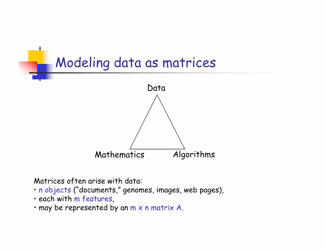
Modeling data as matrices

Data

Matrices often arise with data: • n objects (“documents,” genomes, images, web pages), • each with m features,• may be represented by an m x n matrix A.

Mathematics Algorithms

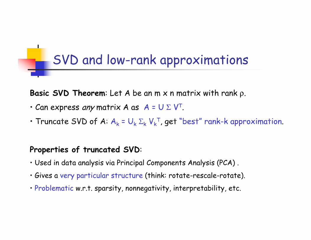
SVD and low-rank approximations

Basic SVD Theorem: Let A be an m x n matrix with rank ρ.

• Can express any matrix A as A = U Σ VT.

• Truncate SVD of A: Ak = Uk Σk VkT, get “best” rank-k approximation. • Truncate SVD of A: Ak = Uk Σk VkT, get “best” rank-k approximation.

Properties of truncated SVD:

• Used in data analysis via Principal Components Analysis (PCA) .

• Gives a very particular structure (think: rotate-rescale-rotate).

• Problematic w.r.t. sparsity, nonnegativity, interpretability, etc.

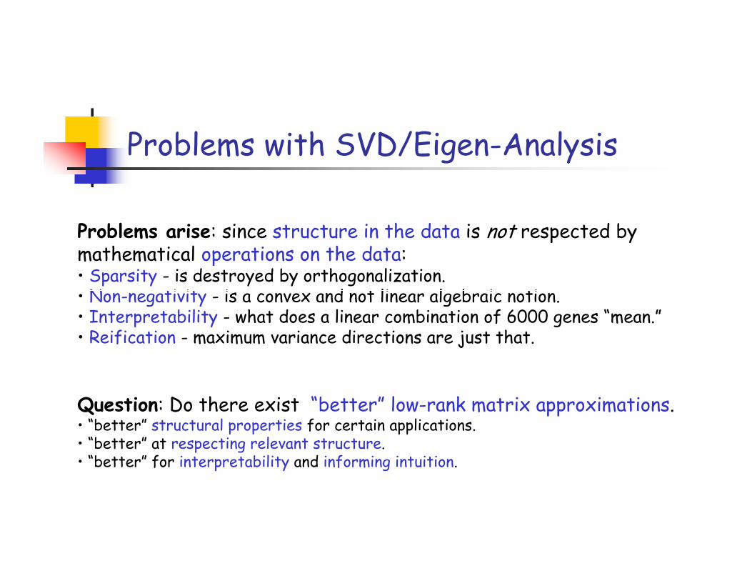
Problems with SVD/Eigen-Analysis

Problems arise: since structure in the data is not respected by mathematical operations on the data: • Sparsity - is destroyed by orthogonalization.• Non-negativity - is a convex and not linear algebraic notion.• Non-negativity - is a convex and not linear algebraic notion.• Interpretability - what does a linear combination of 6000 genes “mean.”• Reification - maximum variance directions are just that.

Question: Do there exist “better” low-rank matrix approximations. • “better” structural properties for certain applications.• “better” at respecting relevant structure.• “better” for interpretability and informing intuition.

CX and CUR matrix decompositions

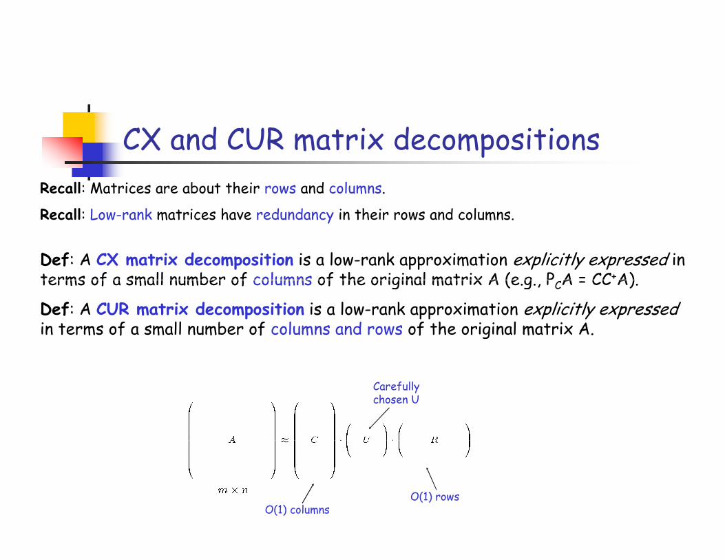
Recall: Matrices are about their rows and columns.

Recall: Low-rank matrices have redundancy in their rows and columns.

Def: A CX matrix decomposition is a low-rank approximation explicitly expressed in terms of a small number of columns of the original matrix A (e.g., PCA = CC+A).

O(1) columnsO(1) rows

Carefully chosen U

terms of a small number of columns of the original matrix A (e.g., PCA = CC+A).

Def: A CUR matrix decomposition is a low-rank approximation explicitly expressedin terms of a small number of columns and rows of the original matrix A.

Two CUR Theorems

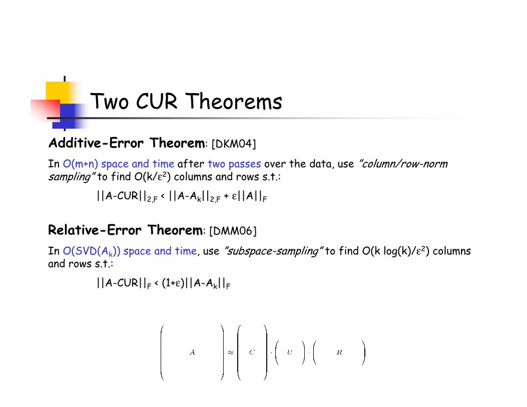
Additive-Error Theorem: [DKM04]

In O(m+n) space and time after two passes over the data, use ”column/row-norm sampling” to find O(k/ε2) columns and rows s.t.:

||A-CUR||2,F < ||A-Ak||2,F + ε||A||F2,F k 2,F F

Relative-Error Theorem: [DMM06]

In O(SVD(Ak)) space and time, use ”subspace-sampling” to find O(k log(k)/ε2) columns and rows s.t.:

||A-CUR||F < (1+ε)||A-Ak||F

Previous CUR-type decompositionsGoreinov, Tyrtyshnikov, &

Zamarashkin

(LAA ’97, …)

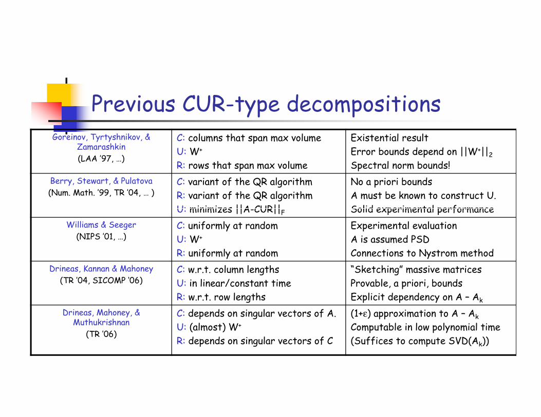
C: columns that span max volume

U: W+

R: rows that span max volume

Existential result

Error bounds depend on ||W+||2Spectral norm bounds!

Berry, Stewart, & Pulatova

(Num. Math. ’99, TR ’04, … )C: variant of the QR algorithm

R: variant of the QR algorithm

U: minimizes ||A-CUR||F

No a priori bounds

A must be known to construct U.

Solid experimental performanceU: minimizes ||A-CUR||F Solid experimental performance

Williams & Seeger

(NIPS ’01, …)C: uniformly at random

U: W+

R: uniformly at random

Experimental evaluation

A is assumed PSD

Connections to Nystrom method

Drineas, Kannan & Mahoney

(TR ’04, SICOMP ‘06)C: w.r.t. column lengths

U: in linear/constant time

R: w.r.t. row lengths

“Sketching” massive matrices

Provable, a priori, bounds

Explicit dependency on A – AkDrineas, Mahoney, & Muthukrishnan

(TR ’06)

C: depends on singular vectors of A.

U: (almost) W+

R: depends on singular vectors of C

(1+ε) approximation to A – AkComputable in low polynomial time

(Suffices to compute SVD(Ak))

Three CUR Data Applications

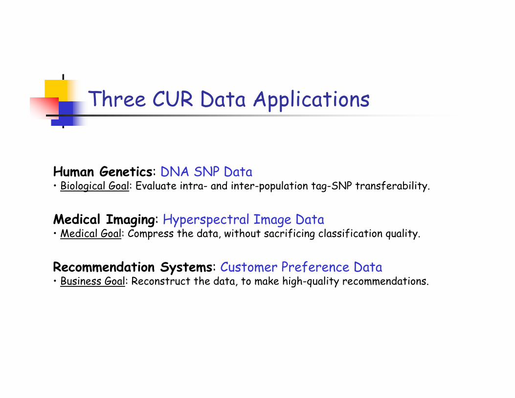
Human Genetics: DNA SNP Data• Biological Goal: Evaluate intra- and inter-population tag-SNP transferability.

Medical Imaging: Hyperspectral Image Data• Medical Goal: Compress the data, without sacrificing classification quality.

Recommendation Systems: Customer Preference Data• Business Goal: Reconstruct the data, to make high-quality recommendations.

CUR Data Application: Human Genetics

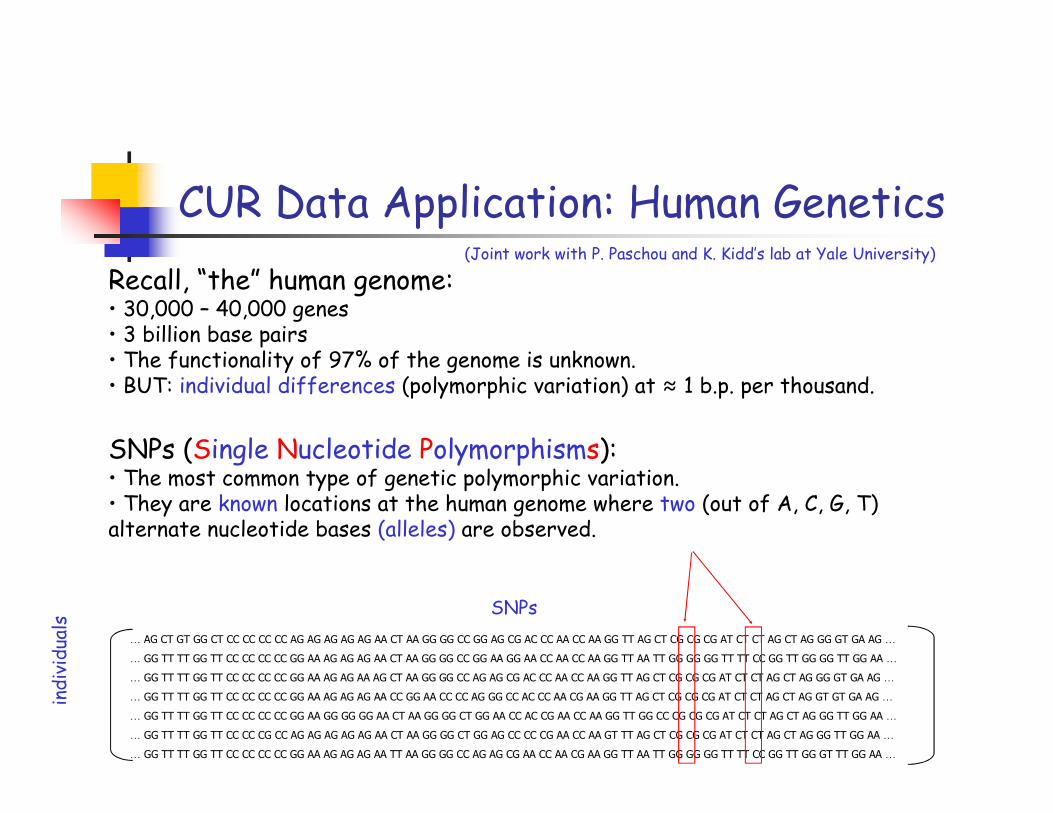
Recall, “the” human genome: • 30,000 – 40,000 genes• 3 billion base pairs• The functionality of 97% of the genome is unknown. • BUT: individual differences (polymorphic variation) at ≈ 1 b.p. per thousand.

(Joint work with P. Paschou and K. Kidd’s lab at Yale University)

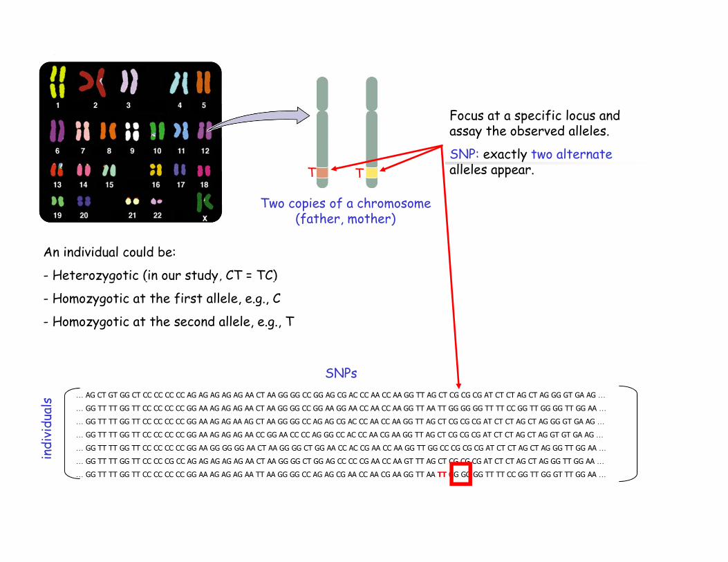
SNPs (Single Nucleotide Polymorphisms): • The most common type of genetic polymorphic variation.• They are known locations at the human genome where two (out of A, C, G, T) alternate nucleotide bases (alleles) are observed.

SNPs

individuals

… AG CT GT GG CT CC CC CC CC AG AG AG AG AG AA CT AA GG GG CC GG AG CG AC CC AA CC AA GG TT AG CT CG CG CG AT CT CT AG CT AG GG GT GA AG …

… GG TT TT GG TT CC CC CC CC GG AA AG AG AG AA CT AA GG GG CC GG AA GG AA CC AA CC AA GG TT AA TT GG GG GG TT TT CC GG TT GG GG TT GG AA …

… GG TT TT GG TT CC CC CC CC GG AA AG AG AA AG CT AA GG GG CC AG AG CG AC CC AA CC AA GG TT AG CT CG CG CG AT CT CT AG CT AG GG GT GA AG …

… GG TT TT GG TT CC CC CC CC GG AA AG AG AG AA CC GG AA CC CC AG GG CC AC CC AA CG AA GG TT AG CT CG CG CG AT CT CT AG CT AG GT GT GA AG …

… GG TT TT GG TT CC CC CC CC GG AA GG GG GG AA CT AA GG GG CT GG AA CC AC CG AA CC AA GG TT GG CC CG CG CG AT CT CT AG CT AG GG TT GG AA …

… GG TT TT GG TT CC CC CG CC AG AG AG AG AG AA CT AA GG GG CT GG AG CC CC CG AA CC AA GT TT AG CT CG CG CG AT CT CT AG CT AG GG TT GG AA …

… GG TT TT GG TT CC CC CC CC GG AA AG AG AG AA TT AA GG GG CC AG AG CG AA CC AA CG AA GG TT AA TT GG GG GG TT TT CC GG TT GG GT TT GG AA …

SNP Biology

SNPs carry redundant information: • Human genome is organized into block-like structure.• Strong, but nontrivial, intra-block correlations.• Can focus only on “tagging SNPs,” or tSNPs.

Different patterns of SNP frequencies/correlations in different populations (e.g., European, Asian, African, etc.): • Can track population histories and disease genes.• Effective markers for genomic research.

International HapMap Project: • Create a haplotype map of human genetic variability.• Map all 10,000,000 SNPs for 270 individuals from 4 different populations.

SNP Pharmacology

Disease association studies: • Locate causative genes for common complex disorders (e.g., diabetes, heart disease).• Identify association between affection status and known SNPs. • Don’t need: knowledge of function of the genes or etiology of the disorder.• Investigate candidate genes in physical proximity with associated SNPs.• Investigate candidate genes in physical proximity with associated SNPs.

Develop the “next generation” of drugs: • “population-specific,” eventually “genome-specific,” not just “disease-specific”.

Funding: • HapMap project (~$100,000,000 from NIH, etc.).• Funding also from pharmaceutical companies, NSF, the DOJ*, etc.

*Is it possible to identify the ethnicity of a suspect from his DNA?

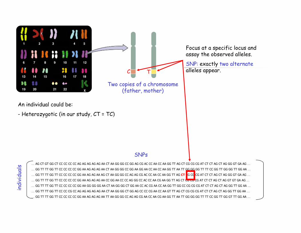
Focus at a specific locus and assay the observed alleles.

SNP: exactly two alternatealleles appear.

Two copies of a chromosome (father, mother)

C T

An individual could be:

- Heterozygotic (in our study, CT = TC)

SNPs

individuals









C C






SNPs

individuals









- Homozygotic at the first allele, e.g., C

T T






SNPs

individuals









- Homozygotic at the first allele, e.g., C

- Homozygotic at the second allele, e.g., T

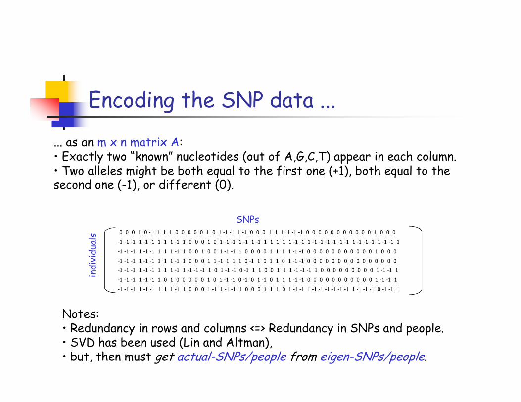
Encoding the SNP data ...

... as an m x n matrix A: • Exactly two “known” nucleotides (out of A,G,C,T) appear in each column.• Two alleles might be both equal to the first one (+1), both equal to the second one (-1), or different (0).

Notes: • Redundancy in rows and columns <=> Redundancy in SNPs and people.• SVD has been used (Lin and Altman), • but, then must get actual-SNPs/people from eigen-SNPs/people.

SNPs

individuals

0 0 0 1 0 -1 1 1 1 0 0 0 0 0 1 0 1 -1 -1 1 -1 0 0 0 1 1 1 1 -1 -1 0 0 0 0 0 0 0 0 0 0 0 1 0 0 0

-1 -1 -1 1 -1 -1 1 1 1 -1 1 0 0 0 1 0 1 -1 -1 1 -1 1 -1 1 1 1 1 1 -1 -1 1 -1 -1 -1 -1 -1 -1 1 -1 -1 -1 1 -1 -1 1

-1 -1 -1 1 -1 -1 1 1 1 -1 1 0 0 1 0 0 1 -1 -1 1 0 0 0 0 1 1 1 1 -1 -1 0 0 0 0 0 0 0 0 0 0 0 1 0 0 0

-1 -1 -1 1 -1 -1 1 1 1 -1 1 0 0 0 1 1 -1 1 1 1 0 -1 1 0 1 1 0 1 -1 -1 0 0 0 0 0 0 0 0 0 0 0 0 0 0 0

-1 -1 -1 1 -1 -1 1 1 1 -1 1 -1 -1 -1 1 0 1 -1 -1 0 -1 1 1 0 0 1 1 1 -1 -1 -1 1 0 0 0 0 0 0 0 0 0 1 -1 -1 1

-1 -1 -1 1 -1 -1 1 0 1 0 0 0 0 0 1 0 1 -1 -1 0 -1 0 1 -1 0 1 1 1 -1 -1 0 0 0 0 0 0 0 0 0 0 0 1 -1 -1 1

-1 -1 -1 1 -1 -1 1 1 1 -1 1 0 0 0 1 -1 1 -1 -1 1 0 0 0 1 1 1 0 1 -1 -1 1 -1 -1 -1 -1 -1 -1 1 -1 -1 -1 0 -1 -1 1

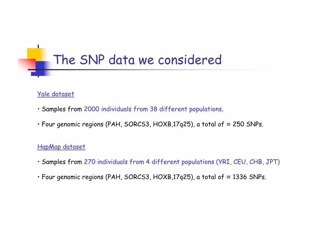
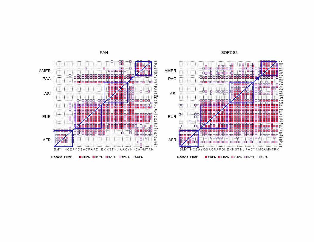
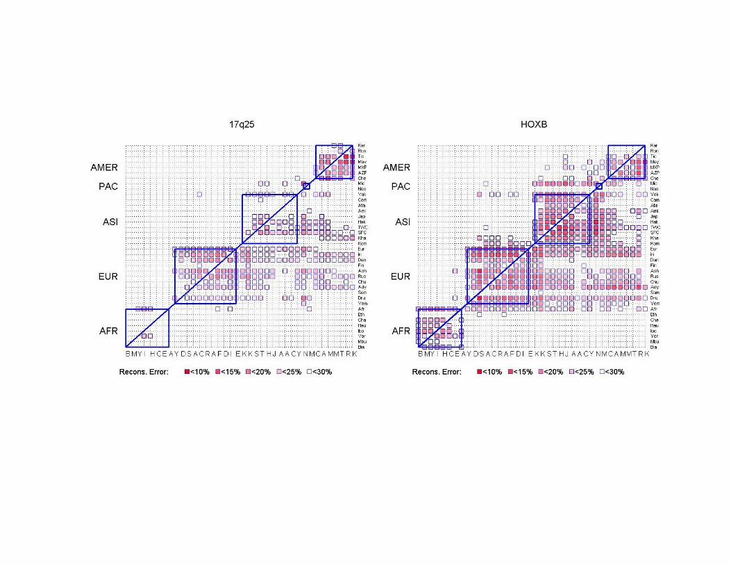
Yale dataset

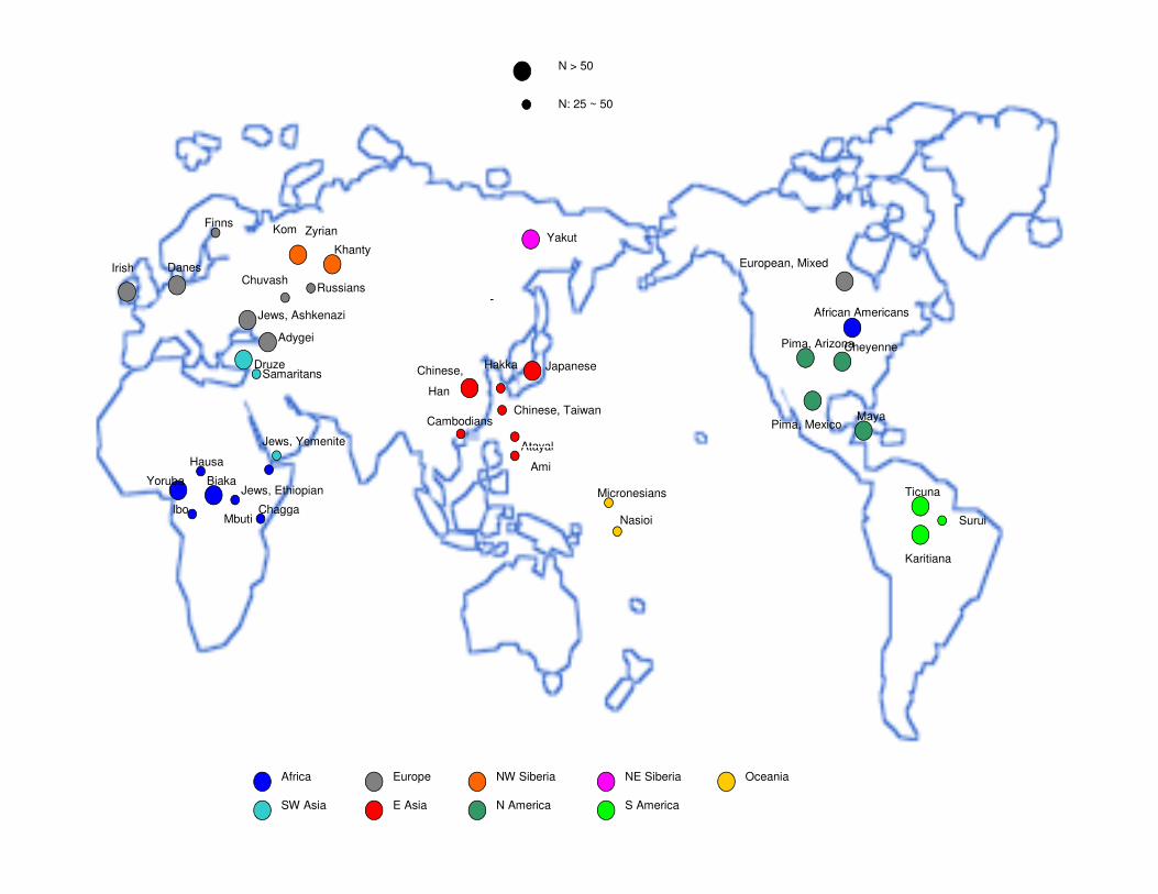
• Samples from 2000 individuals from 38 different populations.

• Four genomic regions (PAH, SORCS3, HOXB,17q25), a total of ≈ 250 SNPs.

The SNP data we considered


HapMap dataset

• Samples from 270 individuals from 4 different populations (YRI, CEU, CHB, JPT)


-African Americans

N > 50

N: 25 ~ 50

Druze

Jews, Yemenite

Samaritans

Adygei

Russians

Finns

DanesIrish European, Mixed

Chuvash

Chinese, Taiwan

Chinese,

Han

Hakka Japanese

Atayal

Cambodians

YakutKom

-

Zyrian

Khanty

Jews, Ashkenazi

Pima, Arizona

Pima, Mexico

Cheyenne

Maya

Yoruba Biaka

MbutiIbo

Hausa

Jews, Ethiopian

Chagga

Africa

SW Asia

Jews, Yemenite

Europe

Atayal

Ami

E Asia

NW Siberia NE Siberia Oceania

Micronesians

Nasioi

N America S America

Ticuna

Surui

Karitiana

Predicting SNPs within a population

Split each population: training and test sets.

Goal: Given SNP information for all individuals in the training set AND for a small number of SNPs for all individuals (tagging-SNPs), predict all unassayed SNPs.

Note: Tagging-SNPs are selected using only the training set. Note: Tagging-SNPs are selected using only the training set.

SNPs

individuals

“Training” set

chosen uniformly at random

(for a few individuals, we are given all SNPs)

SNP sample

(for all subjects, we are given a small number of SNPs)

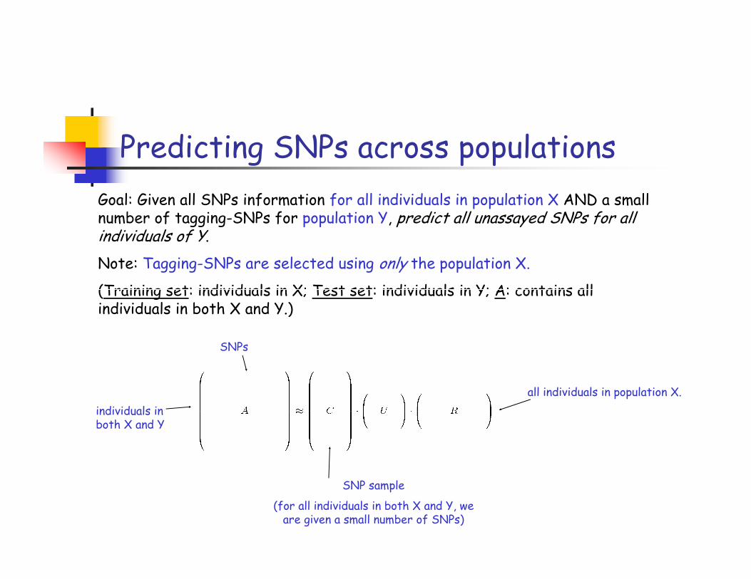
Predicting SNPs across populations

Goal: Given all SNPs information for all individuals in population X AND a small number of tagging-SNPs for population Y, predict all unassayed SNPs for all individuals of Y.

Note: Tagging-SNPs are selected using only the population X.

(Training set: individuals in X; Test set: individuals in Y; A: contains all (Training set: individuals in X; Test set: individuals in Y; A: contains all individuals in both X and Y.)

SNPs

individuals in both X and Y

all individuals in population X.

SNP sample

(for all individuals in both X and Y, we are given a small number of SNPs)

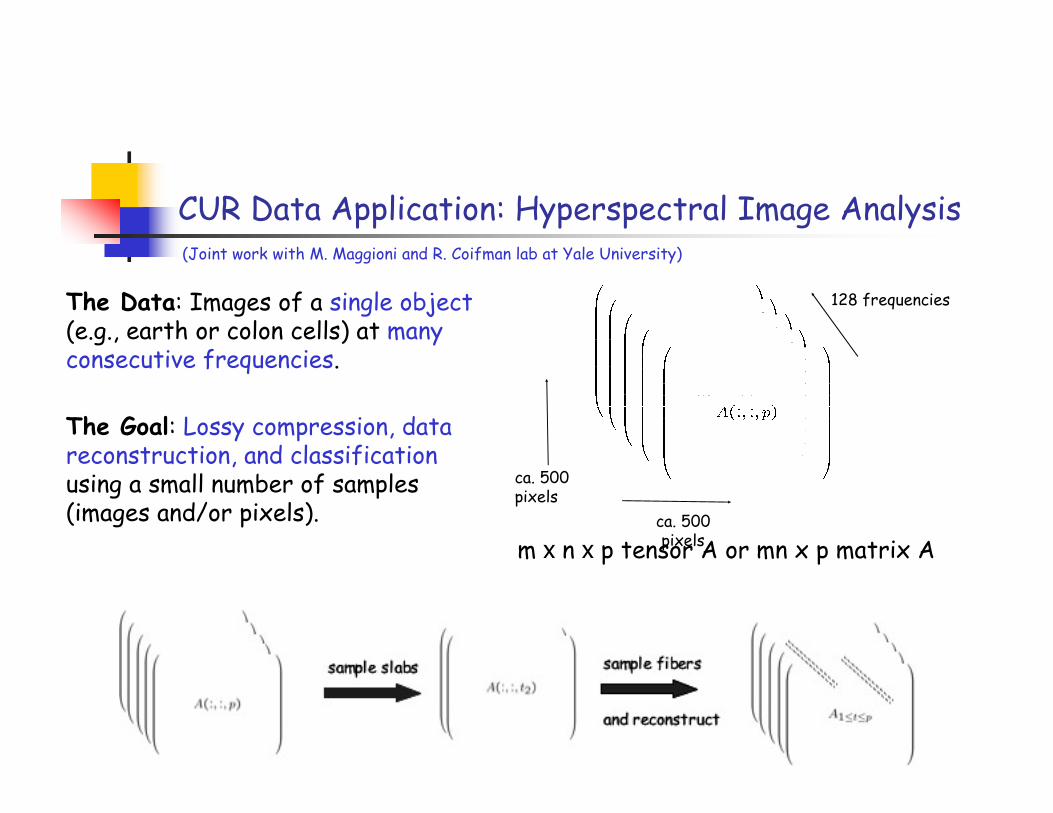
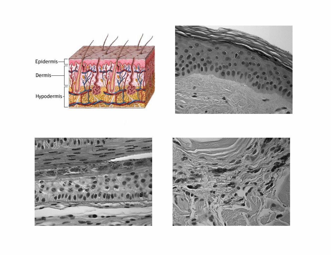
CUR Data Application: Hyperspectral Image Analysis

The Data: Images of a single object(e.g., earth or colon cells) at many consecutive frequencies.

128 frequencies

(Joint work with M. Maggioni and R. Coifman lab at Yale University)

The Goal: Lossy compression, data reconstruction, and classificationusing a small number of samples (images and/or pixels). ca. 500

pixels

ca. 500 pixels

m x n x p tensor A or mn x p matrix A

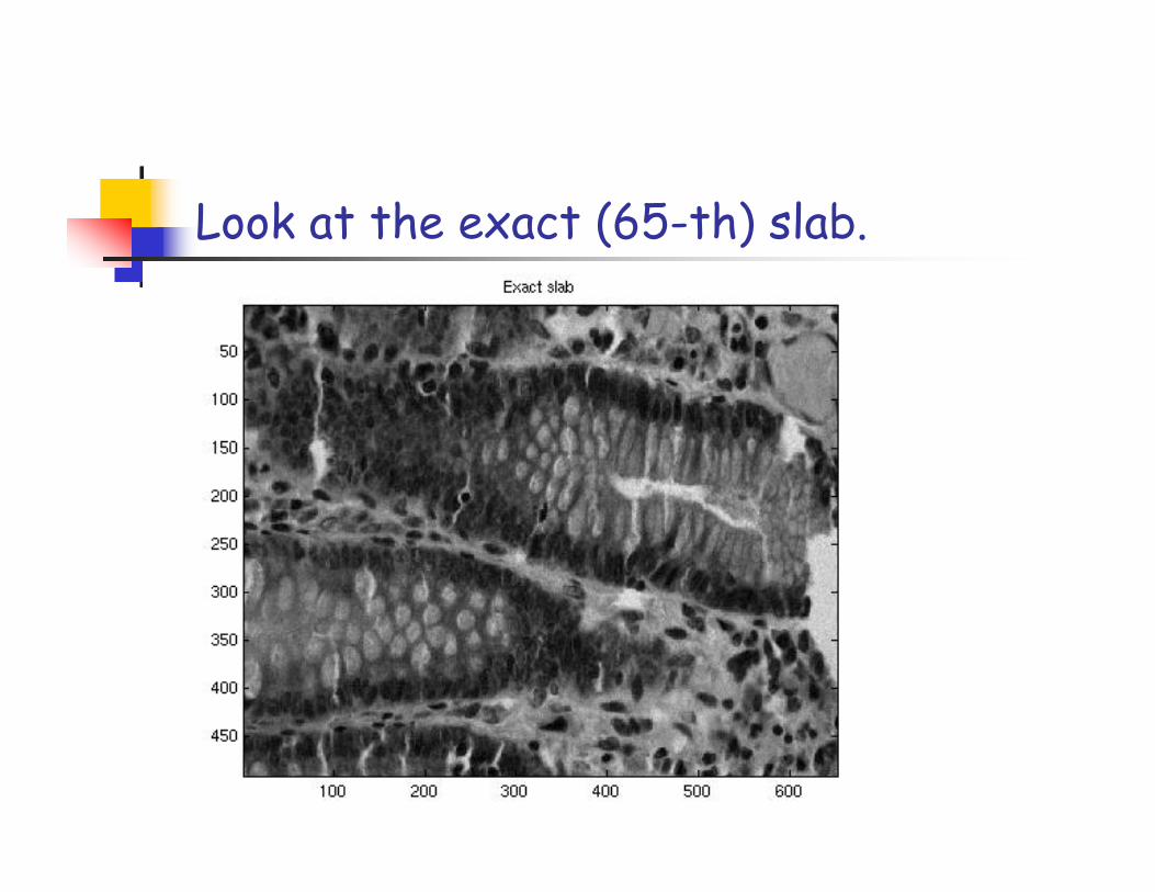
Look at the exact (65-th) slab.

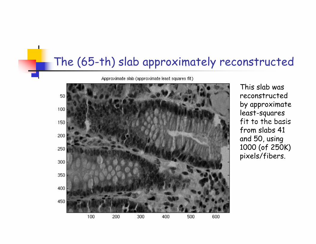
The (65-th) slab approximately reconstructed

This slab was reconstructedby approximate least-squares fit to the basis fit to the basis from slabs 41 and 50, using 1000 (of 250K) pixels/fibers.

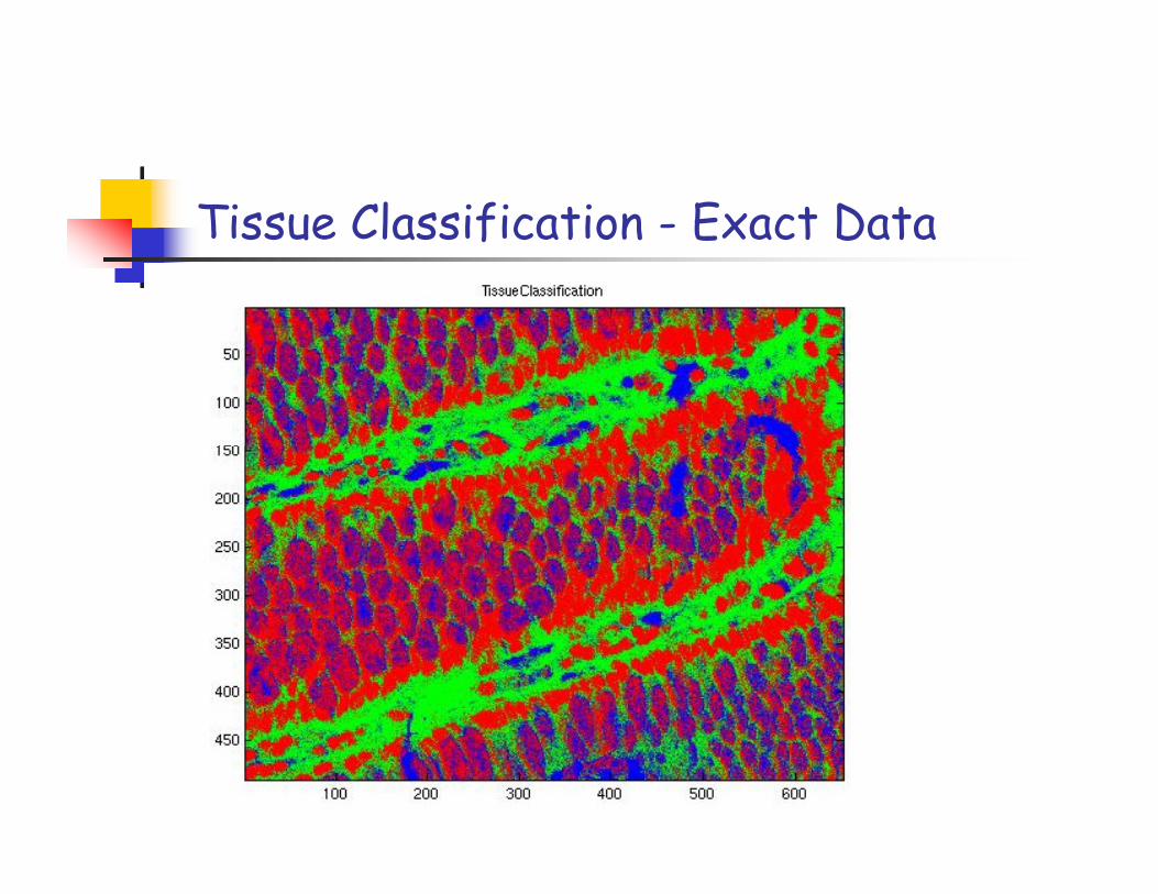
Tissue Classification - Exact Data

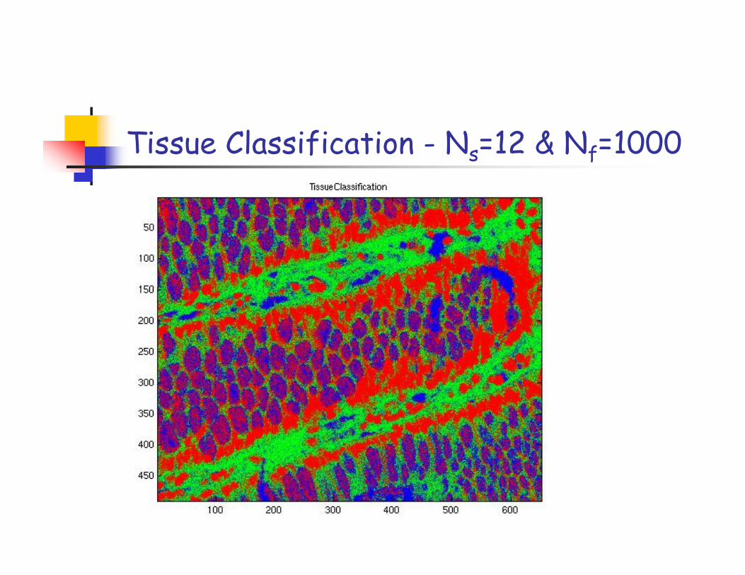
Tissue Classification - Ns=12 & Nf=1000

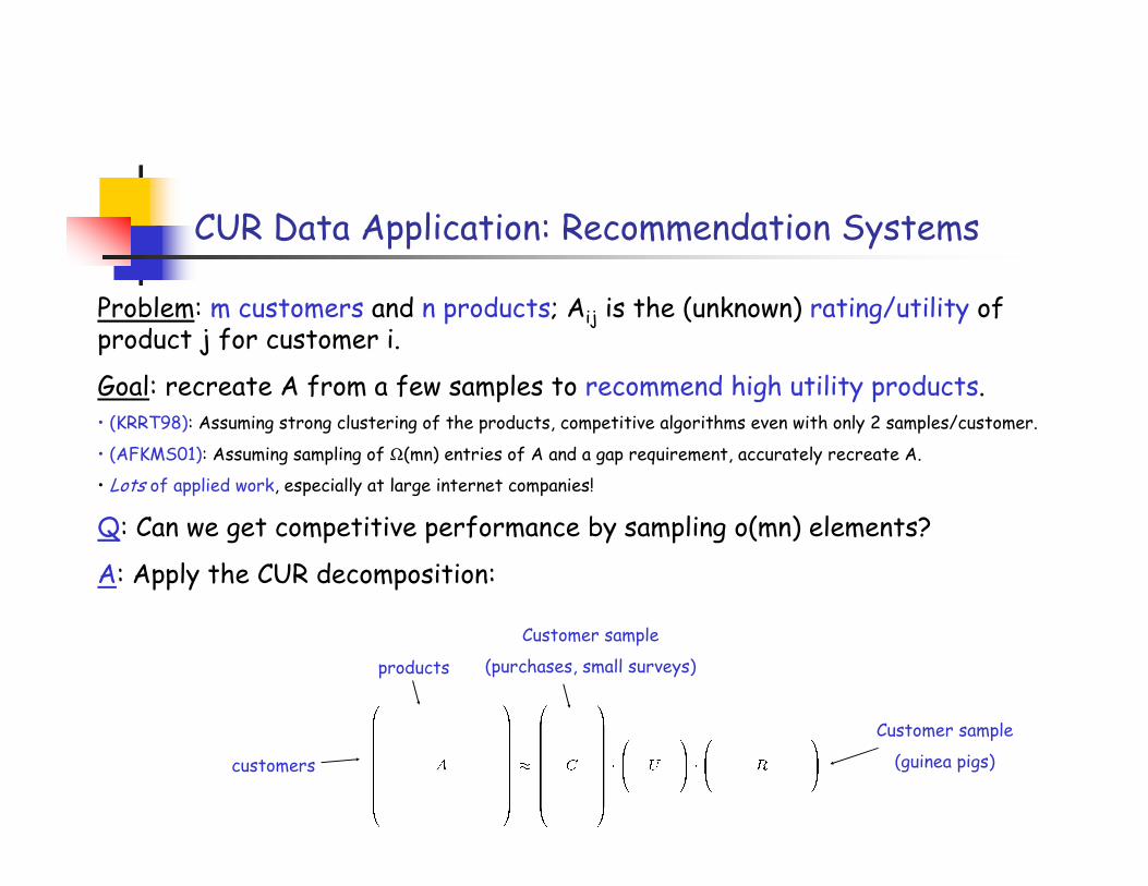
CUR Data Application: Recommendation Systems

Problem: m customers and n products; Aij is the (unknown) rating/utility of product j for customer i.

Goal: recreate A from a few samples to recommend high utility products.• (KRRT98): Assuming strong clustering of the products, competitive algorithms even with only 2 samples/customer.

• (AFKMS01): Assuming sampling of Ω(mn) entries of A and a gap requirement, accurately recreate A.• (AFKMS01): Assuming sampling of Ω(mn) entries of A and a gap requirement, accurately recreate A.

• Lots of applied work, especially at large internet companies!

Q: Can we get competitive performance by sampling o(mn) elements?

A: Apply the CUR decomposition:

products

customers

Customer sample

(guinea pigs)

Customer sample

(purchases, small surveys)

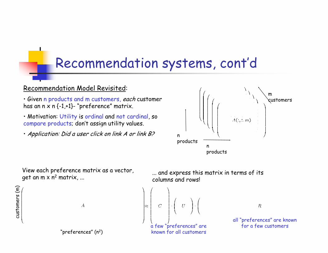
Recommendation systems, cont’d

Recommendation Model Revisited:

• Given n products and m customers, each customer has an n x n -1,+1- “preference” matrix.

• Motivation: Utility is ordinal and not cardinal, so compare products; don’t assign utility values.

m customers

View each preference matrix as a vector, get an m x n2 matrix, ...

“preferences” (n2)

customers (m)

all “preferences” are known for a few customersa few “preferences” are

known for all customers

... and express this matrix in terms of its columns and rows!

compare products; don’t assign utility values.

• Application: Did a user click on link A or link B?

n products

n products

Application to Jester Joke Recommendations

Use just the 14,140 “full” users who rated all 100 Jester jokes.

For each user, convert the utility vector to 100 x 100 pair-wise preference matrix.

Choose, e.g., 300 users (slabs), and a small number of comparisons (fibers).

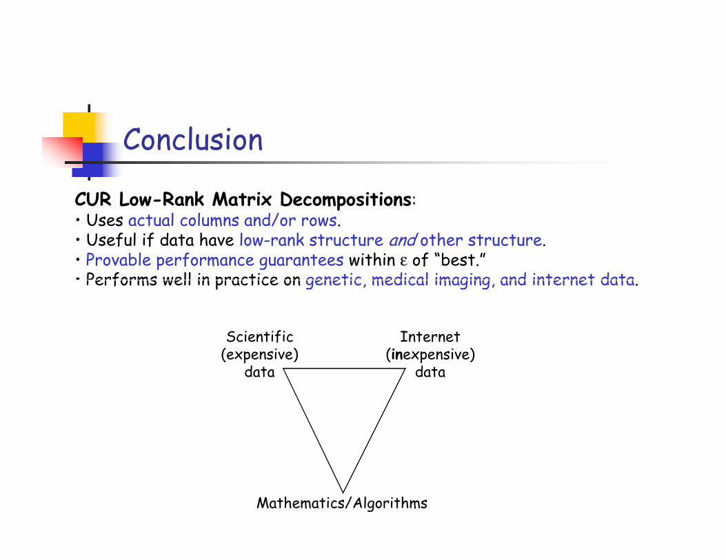
Conclusion

CUR Low-Rank Matrix Decompositions: • Uses actual columns and/or rows.• Useful if data have low-rank structure and other structure.• Provable performance guarantees within ε of “best.”• Performs well in practice on genetic, medical imaging, and internet data.• Performs well in practice on genetic, medical imaging, and internet data.

Scientific (expensive) data

Mathematics/Algorithms

Internet(inexpensive)

data

CUR Matrix Decompositions for Improved Data Analysis · Workshop on Algorithms for Modern Massive...

Documents

Transcript of CUR Matrix Decompositions for Improved Data Analysis · Workshop on Algorithms for Modern Massive...