Munich Personal RePEc Archive

Cupid and Psyche: Cognition and the

Choice of the Partner

Marini, Annalisa

University of Exeter

2017

Online at https://mpra.ub.uni-muenchen.de/99712/

MPRA Paper No. 99712, posted 21 Apr 2020 10:19 UTC

Cupid and Psyche:

Cognition and the Choice of the Partner

Annalisa Marini

University of Exeter ∗

April, 2020

Abstract

The paper provides the first empirical evidence on the importance of cognition - numeric

ability - in the choice of the partner. Using the British Household Panel Study Understand-

ing Society, I estimate a structural model of marriage sorting on a representative sample of

British couples. Results show that partners with similar numeric ability are attracted to each

other. Cognition and physical characteristics are the most important attributes in marriage

sorting. Personality traits and risk propensity are also relevant to various extents. Heteroge-

neous preferences across gender are found and results are robust to an alternative specification.

Implications of mutual attractiveness in cognition for marriage dynamics are discussed.

∗University of Exeter, Streatham Court, Rennes Drive, EX4 4PU, Exeter, UK, e-mail:a.marini@exeter.ac.uk. First draft: September 2017. This paper is an updated version of a pre-vious paper entitled “Who Marries Whom? The Role of Identity, Cognitive and NoncognitiveSkills in Marriage”. I am very grateful to Sonia Oreffice, Climent Quintana-Domeque and Jo Sil-vester for useful suggestions and feedback on an earlier version of the paper. All the remainingerrors are mine. The author declares no conflict of interests.

1

“You are like nobody since I love you”, P. Neruda

“Love is always also an amazing intellectual adventure”, F. Alberoni

“Rare are the people who use their head, few those who use their hearth, and unique

those who use both”, R. Levi Montalcini

“Drink this Psyche and be immortal! Nor shall Cupid ever break away from the knot

in which he is tied, but these nuptials shall be perpetual”, Apuleius

1 Introduction

Marriage may influence happiness, wealth and welfare of the two partners and their offsprings,

therefore, understanding what drives marriage sorting is crucial.

The literature has often considered education, income, and more recently noncognitive skills

to explain marriage matching. I here assess the impact of numeric ability, as measure of cognitive

skills. Individuals make use of their numeric ability on a daily basis: these skills relate to and

are among the determinants of various lifetime outcomes involving personal growth, professional

achievements, and decision making broadly defined. Thus, if the assumption that the choice of the

life partner grounds also on mutual attractiveness in cognition holds, then this outcome could have

consequences for dynamic patterns of marriage as well. To the best of my knowledge, no prior

study has investigated the impact of cognition in marriage matching.

Numeric ability is considered across disciplines a good measure for crystallized intelligence.

According to the theory developed in psychology (e.g., Horn and Cattell, 1966; Horn, 1985; Cat-

tell, 1987), crystallized intelligence is one of the dimensions, together with fluid intelligence, that

constitute the two main components of individual primary abilities. Fluid intelligence is compre-

hensive of the factors that can be defined as biological, such as genetically inherited intelligence

and physical injuries/events that may alter intelligence, and abstract thinking; instead, crystallized

intelligence is comprehensive of the factors acquired with experience that may influence intelli-

2

gence, such as for instance education and learning across the life span. Thus, crystallized intelli-

gence is related to individual education, but it is inclusive of acculturated knowledge from daily

life experience, then it is dynamically evolving over time, and, in sharp contrast to other cognitive

skills (e.g., memory), it is increasing over adulthood.

I estimate a static model of marriage sorting as in Dupuy and Galichon (2014) where I let sort-

ing be based on multiple attributes, among which numeric ability. I conduct the analysis using the

years 2009-2011 of the British Household Panel Study - Understanding Society (BHPSUS here-

after) data set. The BHPSUS is a survey representative of the British population that is particularly

suitable to study marriage matching because it provides information about both physical and be-

havioral characteristics of individuals and their partners. Given the availability of similar national

surveys, these features make the paper suitable to be used for cross-country comparison.

The results are as follows. First, physical and mental attraction are the major drivers of mar-

riage sorting: candidate partners with similar crystallized intelligence are mutually attracted to

each other, this characteristic is second only to height, and it is followed by body mass index

(henceforth BMI). Second, risk propensity and the ’Big 5’ personality traits are also relevant to

marriage sorting and support the existing literature, according to which some of these traits are

more relevant than others to explain individual behavior: risk, conscientiousness, openness to ex-

perience and neuroticism are more relevant than extraversion and agreeableness. Third, attributes

have both a direct and indirect -through their interactions- influence on matching. Fourth, the find-

ings suggest the presence of heterogeneous preferences between husbands and wives in the choice

of the partner. Finally, the results are robust to the inclusion of education among the attributes.

The paper is structured as follows. Section 2 motivates the study. Section 3 describes the

data and the empirical methodology. Section 4 reports the results and the alternative specification.

Finally, section 5 presents a discussion and concluding remarks.

3

2 Intelligence of Individuals and Couples

Numeric ability has already been used by researchers across disciplines to analyze individual be-

havior and its consequences. Existing studies (see for instance McArdle et al., 2002; Peters et al.,

2006; Banks and Oldfield, 2007; Smith, McArdle and Willis, 2010; Benjamin, Brown and Shapiro,

2013; Zaval et al., 2015; Chen et al., 2019) have found that individuals with high numeric ability

perform well in a series of tasks and situations, among which discounting, financial literacy, wealth

accumulation, savings and investment, and taking care of their physical health; also, the advantage

of these individuals with respect to those with lower numeric ability is considerable and can lead to

significantly better achievements. Individuals scoring high in crystallized intelligence are generally

more reflexive, more patient, and wiser than the others. They are more likely to think efficiently, to

view problems from different perspectives, they are more capable to exclude irrelevant alternatives

and to process and acknowledge their limited information when making decisions.

Thus, our assumption that individuals choose someone with numeric ability similar to their own

one to form a family, if met, may reinforce this mechanism through interactions and externalities,

amplifying further its impact.

3 Empirical Framework and Data

3.1 Empirical Framework

The model I estimate in the next section grounds on Dupuy and Galichon (2014),1 who extend the

Choo and Siow (2006) marriage model, where marriage matching is based on discrete attributes,

to include continuous attributes.

Males and females, denoted respectively with m and w, search for a partner in the set of their

acquaintances, indexed respectively by k ∈N and l ∈N. The search leads to a one-to-one bipartite

matching model with transferable utility, after couples are matched the number of males and fe-

1I here provide a brief presentation of the methodology, please see Dupuy and Galichon (2014)for details and proofs.

4

males in the sample is the same. Each male has a series of attributes x ∈ X = Rdx and each female

has attributes y ∈ Y = Rdy.

A male and a female will match when the matching, namely, the probability density that a cou-

ple with certain attributes is formed, maximizes the total utility of the couple. Formally, the utility

of a man m with attributes xm = x matching with a woman w with attributes ymk is U

(

x,ymk

)

+ σ2

εmk

and similarly the utility of a woman w with attributes yw = y matching with a man m with at-

tributes x is V(

xwl ,y

)

+ σ2

ηwl , where U

(

x,ymk

)

and V(

xwl ,y

)

are the utilities based on the observ-

able attributes of the potential partner, σ is a parameter that measures intensity of unobserved

heterogeneity, and εmk and ηw

l are the two sympathy shocks for respectively candidate husbands

and candidate wives, {(yml ,ε

ml ),k ∈ M} is Poisson distributed with intensity dy× ε−εdε (the same

applies to the other partner with a change in notation). Dupuy and Galichon (2014) show that this

framework leads to a continuos multinomial logit model.

The two probability distributions for males and females choosing a partner with attributes x

and y are, respectively:

πY |X(y|x) =exp[U(x,y)/(σ/2)]

∫

Y

exp[U(x,y′)/(σ/2)]dy′(1)

and

πX |Y (x|y) =exp[V (x,y)/(σ/2)]

∫

X

exp[V (x′,y)/(σ/2)]dx′. (2)

The maximization problem is as follows:

maxπ∈M(P,Q)

∫ ∫

X×Y

Φ(x,y)π(x,y)dxdy−σ∫ ∫

X×Y

logπ(x,y)π(x,y)dxdy (3)

namely, the maximization of the utility function subject to the probability the matching occurs. In

this optimization problem, Φ(x,y) is the joint utility and it is the sum of the utilities of the two

partners, π(x,y) is the probability distribution that a couple with characteristics (x,y) is formed,

σ is the parameter that measures the intensity of unobserved heterogeneity and P and Q are the

probability distributions of the attributes of males and females. The continuous multinomial logit

5

guarantees independence across disjoint subsets (i.e., the independence of irrelevant alternatives),

which allows to rule out the presence of a systematic sympathy shock (i.e., correlated sympathy

shock across observables) for both candidate partners. It could be appropriate to accommodate

a random sympathy shock for attributes, because of partner preferences; however, if most of the

matching is determined through observables, the impact of unobservables in marriage sorting can

be considered negligible.

The maximization process allows to derive the two equilibrium utilities for husbands and wives;

the equilibrium matching is unique and stable (i.e., no partner prefers another matching) and it

maximizes social gains.

Dupuy and Galichon (2014) show that, under a quadratic parametrization assumption of the

utility function, Φ(x,y), which can be written as ΦA(x,y) = x′Ay, where A, a dx ×dy matrix, is the

affinity matrix whose elements are defined as

Ai j =∂ 2

Φ(x,y)

∂xi∂y j, (4)

the cross-derivative allows the researcher to identify mutual attractiveness.2 When an element of

the matrix is positive, there is positive assortative matching (i.e., complementarity) between the at-

tributes of the husband and the wife, while when the element of the affinity matrix is negative there

is negative assortative matching (i.e., the attributes of the two partners are substitutes). The asym-

metry of the affinity matrix indicates the presence of heterogeneous preferences between candidate

husbands and wives in the matching process. Finally, the structural approach, by controlling for

marginal distributions controls for the possible presence of misleading results due to correlations

across variables.

Once the matrix has been estimated it is possible to conduct a saliency analysis, a method pro-

posed by Dupuy and Galichon (2014) that consists in performing a singular value decomposition

2Note it is impossible to identify absolute attractiveness. Identification can be reached up to a

separable additive function; only the cross-derivative ∂ 2φ (x,y)/∂x∂y, whose elements constitutethe affinity matrix, Ai j, can be identified, while we cannot identify the first derivatives with respectto x and y.

6

of the renormalized affinity matrix. Saliency analysis allows to determine the attributes on which

the marriage sorting decision of couples is based and the indices of mutual attractiveness, namely,

pairs of indices for the two partners explaining a mutually exclusive part of the joint utility.

3.2 Data

The British Household Panel Study Understanding Society data set (BHPSUS) is one of the na-

tional surveys conducted in various countries (other examples are the American Panel Study of

Income Dynamics (PSID), the German SocioEconomic Panel (GSOEP) and the DNB Household

Survey (DHS)) that not only include demographics of the interviewed individuals, but also have

records of physical characteristics, such as for instance height and BMI, and personality traits, that

can be crucial to understand individual behavior, such as who marries whom.

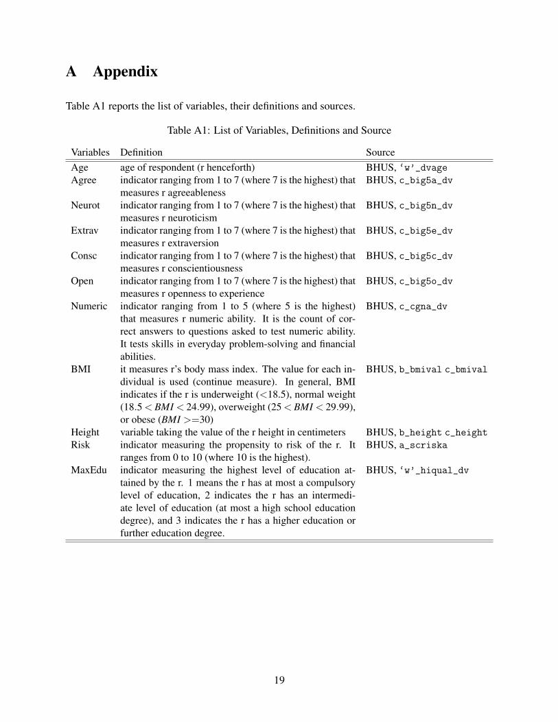
The attributes I use to study marriage sorting are as follows: Numeric Ability as measure for

cognitive skills, height, body mass index (BMI), the Big 5 personality Traits (Conscienciousness,

Extraversion, Agreableeness, Neuroticism, Openness to Experience), risk propensity and later in

the paper the maximum level of education.3

Numeric ability (Numeric) takes values from 0 to 5 and it is a count of the number of problems

the respondent has been able to solve. Following the literature (e.g., Dupuy and Galichon, 2014)

I also use the maximum level of education attained by each individual (MaxEdu), which ranges

from 1 to 3, where it takes value 1 if the individual has almost some degree of compulsory ele-

mentary education, 2 some intermediate level of education (i.e., a high school degree) and 3 higher

education or any further higher education.

The ‘Big 5’ personality traits are measures for noncognitive skills: Conscienciousness, Ex-

traversion, Agreableeness, Neuroticism (or Emotional Stability, depending on how the question is

formulated in each survey), and Openness to Experience. They range from 1 to 7, where 1 cor-

3In the main analysis I omit the maximum level of education because it could be questionedthat the joint utilization of numeric ability and education may generate collinearity problems; how-ever, I provide estimation results also including educational attainment in order to show that therelevance of numeric ability is not a result of its omission.

7

responds to the lowest value and 7 to the highest value of each trait. Conscientiousness (Consc)

captures the ability to self-discipline, to stay focused of a person, to comply with rules and to plan

in advance. Openness to experience (Open) measures the extent to which a person is open to some-

thing new, the need for intellectual stimulation and imagination. Extraversion (Extrav) catches the

degree of interaction with others, the tendency to be involved in social activity and warmth of a

person. Neuroticism (here Neurot) measures anxiety, depression and how well individuals can

control their emotions under stress. Finally, Agreeableness (Agree) measures the tendency to trust

others, altruism, cooperation, and the ability of a person to have harmonious and balanced relations

with other individuals. In line with the previous work (Dupuy and Galichon, 2014) I also control

for risk taking propensity of each person. Risk takes values from 1 to 10, where 1 corresponds to

the lowest value for propensity and 10 to the highest.

Following the marriage literature I also consider height of the individuals (Height, expressed in

centimeters) and the value of the Body Mass Index (BMI). This index captures the extent to which

an individual is underweight (a BMI < 18.5), normal weight (18.5 ≤ BMI < 24.99), overweight

(25 ≤ BMI < 29.99) or obese (BMI ≥ 30). In the regression I will use the exact value of BMI

(continuous measure) for each individual.

To conduct the analysis, I need information for all the variables used for both males and fe-

males. In order to retrieve values for all the attributes I use the first three waves of the BHPSUS,

corresponding to the years 2009-2011;4 then, I keep the couples for which I have full informa-

tion about the attributes, and I preserve the first year for each couple. I also restrict the sample

to couples whose partners’ age ranges between 18 and 44, so to offset the structural differences

in marriage sorting over time. Thus, the sample starts with 31,023 couples, that reduce to 8,712

after eliminating the couples for which numeric ability, BMI and Height are missing, and to 4,876

after eliminating the missing values for the remaining attributes. Finally, imposing the age limit

leads to a further reduction in the number of couples, which reduce to 1,487, that is, 2,974 indi-

4While some of the variables used are available in a single wave (e.g., noncognitive skills),others may be observed over multiple waves (i.e., education and BMI). For these attributes I useeither the individual average or the maximum value across the available values. This does notaffect the results because they are computed using values from 1 to at most 3 consecutive years.

8

viduals. As it is generally the case for survey data, it should be reckoned that also the BHPSUS is

affected by attrition; the attributes are standardized in the structural estimation, as in Dupuy and

Galichon (2014), to make results comparable across attributes. The variables, their source and their

definition are presented in the Appendix.

4 Results

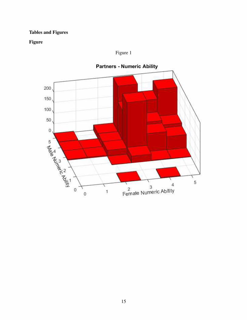
Figure 1 presents a first preliminary evidence of our assumption. It shows the repartition of couples

of the BHPSUS sample by their numeric ability.

- Please enter Figure 1 about here -

While, luckily, there are not many individuals and couples who scored low and who are pairing to

each other, the majority of couples have intermediate levels of numeric ability and there is evidence

of mutual attractiveness in this attribute. It is worth noticing that a good proportion of the candidate

partners who scored 5 (the highest value) decided to marry each other.

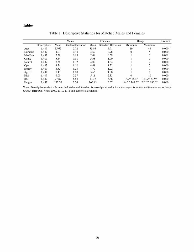
Table 1 presents descriptive statistics for the characteristics of males and females. On aver-

age, husbands are older than wives. Also, the variable for cognitive skills (Numeric), indicates

that husbands have a slight comparative advantage in terms of crystallized intelligence; education

(MaxEdu) is slightly higher for wives: the last two results align to the existing literature suggesting

that females outperform males in educational attainment and a disappearance, in more gender-

equal societies as the United Kingdom, of differences across genders in test performance (The

Department for Education, 2009; Halpern et al., 2007; Guiso et al., 2008; The Department for Ed-

ucation, 2019). In line with the literature (Borghans et al., 2009), the propensity to take risk is

higher for husbands than for wives. Females are more conscientious than males, but also more

neurotic. Openness to experience is slightly higher for husbands, while wives are more extroverted

and also on average more agreeable than husbands. Finally, anthropometrics reflect the genetic

differences across genders, since husbands have higher values of BMI and are overall taller than

wives; furthermore, the BMI index indicates that both husbands and wives are on average slightly

9

overweight because both samples have average values above 25 and below 30, which are respec-

tively the thresholds for overweight and obesity; since the sample is restricted to relatively young

couples, the finding is a further evidence that obesity is a problem in the United Kingdom (e.g.,

OECD, 2017).

- Please enter Table 1 about here -

However, in order to understand whether and the extent to which numeric ability influences mar-

riage sorting a more structural analysis is needed. This analysis is shown in the rest of the paper.

Table 2 presents the results for the estimation of the affinity matrix on the couples of the sample.

- Please enter Table 2 about here -

The on-diagonal entries, which measure the impact of mutual attractiveness in a specific attribute

on the joint utility function, show that all the attributes, but agreeableness and extraversion, are

directly relevant to explain marriage sorting. Numeric ability is one of the characteristics that

most contribute to the joint utility of the couples, second only to Height: increasing height of

both partners by 1 standard deviation increases the joint utility of a couple by 0.28 units, while

increasing cognitive skills increases it by 0.19 units.

The off-diagonal entries show if two given characteristics of the partners are complementary or

substitutes and it represents the importance of cross gender interactions between attributes. Cog-

nition is not only directly but also indirectly important to explain who marries whom; the results

show that, for both partners, there is a trade-off between numeric ability and BMI, that is, there is

a negative interaction between numeric ability of individuals and BMI of their partner. Also, the

asymmetry of the affinity matrix suggests that husbands and wives have different preferences for

attributes of the partner: the joint utility of a couple whose husband is relatively more intelligent

benefits from having a wife that is more open to experience, and husbands’ intelligence interacts

negatively with risk propensity and agreeableness of a wife; instead, wife’s numeric ability neg-

atively interacts with husband’s conscientiousness, and increasing wife’s numeric ability by one

10

standard deviation has the same impact on the joint utility disregarding changes in the remaining

attributes.

Similarly, height of husbands has a negative interaction with conscientiousness of wives and

a positive one with their neuroticism; instead, increasing wife’s height by a standard deviation

increases the joint utility of couples whose husband is more open to experience relatively more (the

entry is 0.09), but there is a negative interaction between wife’s height and husband’s neuroticism

and agreeableness. BMI, the other physical attribute, is also relevant to explain the matching

and the on-diagonal estimated parameter, 0.14, is also among the most sizeable, confirming the

importance of physical characteristics in marriage sorting.

The on-diagonal entry for Risk is also high: with a value of 0.14 this attribute reveals the pres-

ence of positive assortative matching in risk propensity. The negative correlation between risk of

both partners and agreeableness of their respective partner may suggest (although further investi-

gation is needed) that individuals who are relatively more risk lovers do not enjoy the company of

partners that are too compassionate or kind because their behavior may be not stimulating.

Regarding the ‘Big 5’ personality traits, individuals with similar levels of both conscientious-

ness and openness to experience are attracted to each other (both the on-diagonal entries are 0.09);

instead, neuroticism, with an on-diagonal entry of -0.10, is a substitute, suggesting that if a partner

is neurotic the couple is, comprehensively, better off if the other partner is more emotionally sta-

ble. The off-diagonal entries indicate that the personality traits contribute to the joint utility of the

couple also indirectly and suggest that preferences between the two subsamples are heterogeneous.

For instance, increasing husband’s conscientiousness by one standard deviation raises the joint util-

ity of the couple whose wife is more agreeable relatively more (the off-diagonal entry is 0.09), the

interaction between wife’s conscientiousness and husband’s agreeableness is not significant. The

other off-diagonal entries may be similarly interpreted and they also highlight the presence of non

homogeneous preferences across genders. Also, in accord with the existing literature (Borghans

et al., 2008; Dupuy and Galichon, 2014), some personality traits are more relevant than others for

the choice of the partner and the determination of the joint utilty of the couples.

11

In addition, the bottom part of the table reports in Panel A the share of joint utility explained by

the indices, and in Panel B the principal component analysis to investigate how much is explained

by the indices. Panel A shows that most of the indices are statistically significant. Also, the

observables explain the totality of the joint utility, so we can safely assume that the attribute specific

random sympathy shock is negligible; the first four indices explain about the 74 per cent of the total

utility.

In Panel B the principal component analysis suggests that the first index, which explains the

23.32 per cent of the total observed matching utility, loads for both husbands and wives on numeric

ability: this result is a further confirmation of the importance of this attribute for marriage sorting;

instead, the second index loads on physical characteristics and the third index loads on personality.

Thus, all in all, the results show that all the attributes jointly explain, directly and/or indirectly,

the joint utility of the British couples. Besides, the asymmetry of the matrix remarks the presence

of heterogeneous preferences across husbands and wives. The saliency analysis further reinforces

this finding and remarks the relevance of numeric ability in marriage matching.

Finally, Table 3 presents the matrix estimated by adding to the list of attributes the maximum

level of education attained. The table indicates that the results for our variable of interest hold and

are very similar to the entries of Table 2. While now the maximum level of education is, together

with Height, the highest on-diagonal entry, Numeric is the third most important attribute in the

matrix, it is more relevant than Risk and BMI.

- Please enter Table 3 about here -

The saliency analysis for Table 3 is shown at the bottom of the table. Once again, the observables

explain the totality of the joint utility. The first four indices explain about the 70 per cent of the

total utility. The principal component analysis in Panel B confirms that the first index loads on

both MaxEdu and Numeric, confirming the complementarity of these two attributes, and Open; the

second loads on physical characteristics and partly again on Numeric, the third on personality. It

is also interesting that the effect of cognition is smoothed across the three indices. So, this table

confirms that the results in Tables 2 are not driven by the omission of educational attainment.

12

5 Discussion and Conclusions

The paper provides evidence on the impact of cognition in the choice of the partner and shows that

partners with similar numeric ability are attracted to each other. All in all, the findings indicate

that individuals are more likely to marry partners that are similar to them in terms of physical

characteristics, cognition, and personality: there is significant negative assortative matching only

in neuroticism. The attributes are also indirectly relevant, to various extents, for the determina-

tion of the joint utility of the couple; furthermore, the asymmetry of the affinity matrix reveals

heterogeneous preferences in marriage between husbands and wives.

Mutual attractiveness in numeric ability has non-trivial implications for household dynamics.

Individuals with high numeric ability have, generally, qualities that lead them to be successful

in several lifetime outcomes. The evidence produced so far reveals that they have a substantial

comparative advantage with respect to the rest of the population.

Then, our results are compatible with a scenario where differences in success largely vary

between the relatively few families where both partners score high in numeric ability and all the

other families in a population. The divergence is expected to be drastic when we compare families

with the highest score (5) and those where both partners have low scores (e.g., 0 to 2), but they are

likely to be very large also when we compare the couples with the highest scores and those with

intermediate levels. We expect couples with the highest values of numeric ability to be more able,

other things equal, to face shocks, to endure and to be resilient, and to be more likely to detect and

seize the opportunity in several contexts: these predictions are not limited to few situations, such

as the job market and the career path, financial matters, savings and wealth, but they have broad

applicability. For instance, the trade-off found earlier in the paper between numeric ability of both

partners and BMI of their respective partner, highlights that couples with high levels of cognition

are well aware of the importance to stay fit and healthy. So, the results are consistent with an

overall significantly better performance of these couples with respect to all the other couples of the

sample.

Besides, even more importantly, our findings suggest the above differences will be magnified

13

by interactions between the two partners and the externalities they generate. These implications

will not be limited to the life of the two partners as a couple, but they will similarly influence,

through direct socialization, the life of their offsprings, leaving scope for future research.

14

Tables and Figures

Figure

Figure 1

15

Tables

Table 1: Descriptive Statistics for Matched Males and Females

Males Females Range p-values

Observations Mean Standard Deviation Mean Standard Deviation Minimum Maximum

Age 1,487 35.62 5.72 33.86 5.91 19 44 0.000

Numeric 1,487 4.07 0.93 3.62 0.98 0 5 0.000

MaxEdu 1,487 2.39 0.65 2.49 0.59 1 3 0.001

Consc 1,487 5.44 0.98 5.58 1.00 1 7 0.000

Neurot 1,487 3.38 1.32 4.02 1.34 1 7 0.000

Open 1,487 4.76 1.12 4.48 1.22 1 7 0.000

Extrav 1,487 4.52 1.23 4.79 1.22 1 7 0.000

Agree 1,487 5.41 1.00 5.65 1.00 1 7 0.000

Risk 1,487 6.00 2.37 5.11 2.32 0 10 0.000

BMI 1,487 27.89 6.83 27.37 5.86 18.2m 16.4w 163.2m 53.9w 0.000

Height 1,487 177.50 7.74 163.45 6.37 84.2m 144.3w 202.2m 186.6w 0.000

Notes: Descriptive statistics for matched males and females. Superscripts m and w indicate ranges for males and females respectively.

Source: BHPSUS, years 2009, 2010, 2011 and author’s calculation.

16

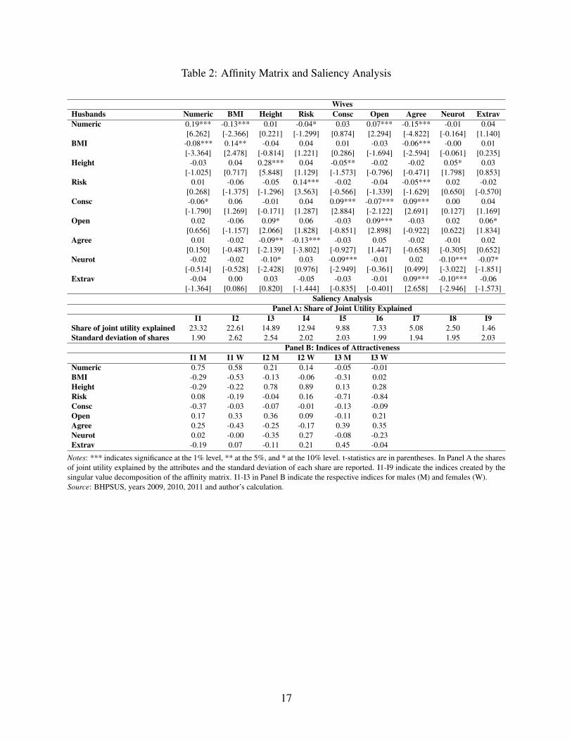
Table 2: Affinity Matrix and Saliency Analysis

Wives

Husbands Numeric BMI Height Risk Consc Open Agree Neurot Extrav

Numeric 0.19*** -0.13*** 0.01 -0.04* 0.03 0.07*** -0.15*** -0.01 0.04

[6.262] [-2.366] [0.221] [-1.299] [0.874] [2.294] [-4.822] [-0.164] [1.140]

BMI -0.08*** 0.14** -0.04 0.04 0.01 -0.03 -0.06*** -0.00 0.01

[-3.364] [2.478] [-0.814] [1.221] [0.286] [-1.694] [-2.594] [-0.061] [0.235]

Height -0.03 0.04 0.28*** 0.04 -0.05** -0.02 -0.02 0.05* 0.03

[-1.025] [0.717] [5.848] [1.129] [-1.573] [-0.796] [-0.471] [1.798] [0.853]

Risk 0.01 -0.06 -0.05 0.14*** -0.02 -0.04 -0.05*** 0.02 -0.02

[0.268] [-1.375] [-1.296] [3.563] [-0.566] [-1.339] [-1.629] [0.650] [-0.570]

Consc -0.06* 0.06 -0.01 0.04 0.09*** -0.07*** 0.09*** 0.00 0.04

[-1.790] [1.269] [-0.171] [1.287] [2.884] [-2.122] [2.691] [0.127] [1.169]

Open 0.02 -0.06 0.09* 0.06 -0.03 0.09*** -0.03 0.02 0.06*

[0.656] [-1.157] [2.066] [1.828] [-0.851] [2.898] [-0.922] [0.622] [1.834]

Agree 0.01 -0.02 -0.09** -0.13*** -0.03 0.05 -0.02 -0.01 0.02

[0.150] [-0.487] [-2.139] [-3.802] [-0.927] [1.447] [-0.658] [-0.305] [0.652]

Neurot -0.02 -0.02 -0.10* 0.03 -0.09*** -0.01 0.02 -0.10*** -0.07*

[-0.514] [-0.528] [-2.428] [0.976] [-2.949] [-0.361] [0.499] [-3.022] [-1.851]

Extrav -0.04 0.00 0.03 -0.05 -0.03 -0.01 0.09*** -0.10*** -0.06

[-1.364] [0.086] [0.820] [-1.444] [-0.835] [-0.401] [2.658] [-2.946] [-1.573]

Saliency Analysis

Panel A: Share of Joint Utility Explained

I1 I2 I3 I4 I5 I6 I7 I8 I9

Share of joint utility explained 23.32 22.61 14.89 12.94 9.88 7.33 5.08 2.50 1.46

Standard deviation of shares 1.90 2.62 2.54 2.02 2.03 1.99 1.94 1.95 2.03

Panel B: Indices of Attractiveness

I1 M I1 W I2 M I2 W I3 M I3 W

Numeric 0.75 0.58 0.21 0.14 -0.05 -0.01

BMI -0.29 -0.53 -0.13 -0.06 -0.31 0.02

Height -0.29 -0.22 0.78 0.89 0.13 0.28

Risk 0.08 -0.19 -0.04 0.16 -0.71 -0.84

Consc -0.37 -0.03 -0.07 -0.01 -0.13 -0.09

Open 0.17 0.33 0.36 0.09 -0.11 0.21

Agree 0.25 -0.43 -0.25 -0.17 0.39 0.35

Neurot 0.02 -0.00 -0.35 0.27 -0.08 -0.23

Extrav -0.19 0.07 -0.11 0.21 0.45 -0.04

Notes: *** indicates significance at the 1% level, ** at the 5%, and * at the 10% level. t-statistics are in parentheses. In Panel A the shares

of joint utility explained by the attributes and the standard deviation of each share are reported. I1-I9 indicate the indices created by the

singular value decomposition of the affinity matrix. I1-I3 in Panel B indicate the respective indices for males (M) and females (W).

Source: BHPSUS, years 2009, 2010, 2011 and author’s calculation.

17

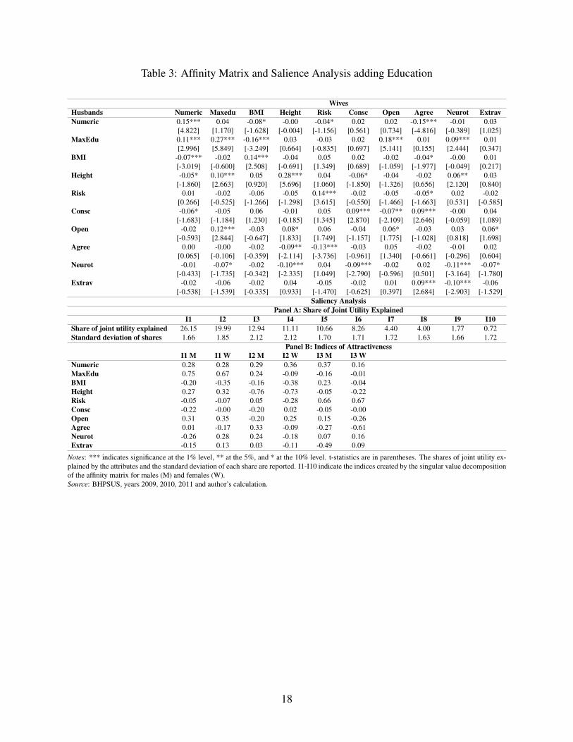
Table 3: Affinity Matrix and Salience Analysis adding Education

Wives

Husbands Numeric Maxedu BMI Height Risk Consc Open Agree Neurot Extrav

Numeric 0.15*** 0.04 -0.08* -0.00 -0.04* 0.02 0.02 -0.15*** -0.01 0.03

[4.822] [1.170] [-1.628] [-0.004] [-1.156] [0.561] [0.734] [-4.816] [-0.389] [1.025]

MaxEdu 0.11*** 0.27*** -0.16*** 0.03 -0.03 0.02 0.18*** 0.01 0.09*** 0.01

[2.996] [5.849] [-3.249] [0.664] [-0.835] [0.697] [5.141] [0.155] [2.444] [0.347]

BMI -0.07*** -0.02 0.14*** -0.04 0.05 0.02 -0.02 -0.04* -0.00 0.01

[-3.019] [-0.600] [2.508] [-0.691] [1.349] [0.689] [-1.059] [-1.977] [-0.049] [0.217]

Height -0.05* 0.10*** 0.05 0.28*** 0.04 -0.06* -0.04 -0.02 0.06** 0.03

[-1.860] [2.663] [0.920] [5.696] [1.060] [-1.850] [-1.326] [0.656] [2.120] [0.840]

Risk 0.01 -0.02 -0.06 -0.05 0.14*** -0.02 -0.05 -0.05* 0.02 -0.02

[0.266] [-0.525] [-1.266] [-1.298] [3.615] [-0.550] [-1.466] [-1.663] [0.531] [-0.585]

Consc -0.06* -0.05 0.06 -0.01 0.05 0.09*** -0.07** 0.09*** -0.00 0.04

[-1.683] [-1.184] [1.230] [-0.185] [1.345] [2.870] [-2.109] [2.646] [-0.059] [1.089]

Open -0.02 0.12*** -0.03 0.08* 0.06 -0.04 0.06* -0.03 0.03 0.06*

[-0.593] [2.844] [-0.647] [1.833] [1.749] [-1.157] [1.775] [-1.028] [0.818] [1.698]

Agree 0.00 -0.00 -0.02 -0.09** -0.13*** -0.03 0.05 -0.02 -0.01 0.02

[0.065] [-0.106] [-0.359] [-2.114] [-3.736] [-0.961] [1.340] [-0.661] [-0.296] [0.604]

Neurot -0.01 -0.07* -0.02 -0.10*** 0.04 -0.09*** -0.02 0.02 -0.11*** -0.07*

[-0.433] [-1.735] [-0.342] [-2.335] [1.049] [-2.790] [-0.596] [0.501] [-3.164] [-1.780]

Extrav -0.02 -0.06 -0.02 0.04 -0.05 -0.02 0.01 0.09*** -0.10*** -0.06

[-0.538] [-1.539] [-0.335] [0.933] [-1.470] [-0.625] [0.397] [2.684] [-2.903] [-1.529]

Saliency Analysis

Panel A: Share of Joint Utility Explained

I1 I2 I3 I4 I5 I6 I7 I8 I9 I10

Share of joint utility explained 26.15 19.99 12.94 11.11 10.66 8.26 4.40 4.00 1.77 0.72

Standard deviation of shares 1.66 1.85 2.12 2.12 1.70 1.71 1.72 1.63 1.66 1.72

Panel B: Indices of Attractiveness

I1 M I1 W I2 M I2 W I3 M I3 W

Numeric 0.28 0.28 0.29 0.36 0.37 0.16

MaxEdu 0.75 0.67 0.24 -0.09 -0.16 -0.01

BMI -0.20 -0.35 -0.16 -0.38 0.23 -0.04

Height 0.27 0.32 -0.76 -0.73 -0.05 -0.22

Risk -0.05 -0.07 0.05 -0.28 0.66 0.67

Consc -0.22 -0.00 -0.20 0.02 -0.05 -0.00

Open 0.31 0.35 -0.20 0.25 0.15 -0.26

Agree 0.01 -0.17 0.33 -0.09 -0.27 -0.61

Neurot -0.26 0.28 0.24 -0.18 0.07 0.16

Extrav -0.15 0.13 0.03 -0.11 -0.49 0.09

Notes: *** indicates significance at the 1% level, ** at the 5%, and * at the 10% level. t-statistics are in parentheses. The shares of joint utility ex-

plained by the attributes and the standard deviation of each share are reported. I1-I10 indicate the indices created by the singular value decomposition

of the affinity matrix for males (M) and females (W).

Source: BHPSUS, years 2009, 2010, 2011 and author’s calculation.

18

A Appendix

Table A1 reports the list of variables, their definitions and sources.

Table A1: List of Variables, Definitions and Source

Variables Definition Source

Age age of respondent (r henceforth) BHUS, ‘w’_dvage

Agree indicator ranging from 1 to 7 (where 7 is the highest) that

measures r agreeableness

BHUS, c_big5a_dv

Neurot indicator ranging from 1 to 7 (where 7 is the highest) that

measures r neuroticism

BHUS, c_big5n_dv

Extrav indicator ranging from 1 to 7 (where 7 is the highest) that

measures r extraversion

BHUS, c_big5e_dv

Consc indicator ranging from 1 to 7 (where 7 is the highest) that

measures r conscientiousness

BHUS, c_big5c_dv

Open indicator ranging from 1 to 7 (where 7 is the highest) that

measures r openness to experience

BHUS, c_big5o_dv

Numeric indicator ranging from 1 to 5 (where 5 is the highest)

that measures r numeric ability. It is the count of cor-

rect answers to questions asked to test numeric ability.

It tests skills in everyday problem-solving and financial

abilities.

BHUS, c_cgna_dv

BMI it measures r’s body mass index. The value for each in-

dividual is used (continue measure). In general, BMI

indicates if the r is underweight (<18.5), normal weight

(18.5 < BMI < 24.99), overweight (25 < BMI < 29.99),

or obese (BMI >=30)

BHUS, b_bmival c_bmival

Height variable taking the value of the r height in centimeters BHUS, b_height c_height

Risk indicator measuring the propensity to risk of the r. It

ranges from 0 to 10 (where 10 is the highest).

BHUS, a_scriska

MaxEdu indicator measuring the highest level of education at-

tained by the r. 1 means the r has at most a compulsory

level of education, 2 indicates the r has an intermedi-

ate level of education (at most a high school education

degree), and 3 indicates the r has a higher education or

further education degree.

BHUS, ‘w’_hiqual_dv

19

References

Banks, J., and Z. Oldfield. 2007. “Understanding Pensions: Cognitive Function, Numerical Abil-

ity and Retirement Saving.” Fiscal Studies, 28(2): 143–170.

Benjamin, D. J., S. A. Brown, and J. M. Shapiro. 2013. “WHO IS ‘BEHAVIORAL’? COGNI-

TIVE ABILITY AND ANOMALOUS PREFERENCES.” Journal of the European Economic

Association, 11(6): 1231–1255.

Borghans, L., A. L. Duckworth, J. J. Heckman, and B. ter Weel. 2008. “The Economics and

Psychology of Personality Traits.” Journal of Human Resources, 43(4): 972–1059.

Borghans, L., B. H. Golsteyn, J. J. Heckman, and H. Meijers. 2009. “Gender Differences

in Risk Aversion and Ambiguity Aversion.” Journal of the European Economic Association,

7(2/3): 649–658.

Cattell, R. B. 1987. Advances in Psychology. Intelligence: Its Structure, Growth, and Action.

Elsevier.

Chen, Y., A. Spagna, T. Wu, T. H. Kim, Q. Wu, C. Chen, Y. Wu, and J. Fan. 2019. “Testing a

Cognitive Control Model of Human Intelligence.” Nature, 9(1): 2898.

Choo, E., and A. Siow. 2006. “Who Marries Whom and Why.” Journal of Political Economy,

114(1): 175–201.

Dupuy, A., and A. Galichon. 2014. “Personality Traits and The Marriage Market.” Journal of

Political Economy, 122(6): 1271–1319.

Guiso, L., F. Monte, P. Sapienza, and L. Zingales. 2008. “Culture, Gender, and Maths.” Science,

320: 1164–1165.

Halpern, D. F., C. P. Benbow, D. C. Geary, R. C. Gur, J. S. Hyde, and M. A. Gernsbacher.

2007. “The Science of Sex Differences in Science and Mathematics.” Psychological Science in

the Public Interest, 8(1): 1–51.

Horn, J. 1985. “Remodeling old models of intelligence: Gf-Gc Theory.” Handbook of Intelligence,

ed. B.B. Wolman, 267–300. New York, Wiley.

Horn, J., and R. Cattell. 1966. “Refinement and Test of the theory of fluid and crystallized intel-

ligence.” Journal of Educational Psychology, 57: 253–270.

McArdle, J. J., E. Ferrer-Caja, F. Hamagami, and R. W. Woodcock. 2002. “Comparative Lon-

gitudinal Structural Analyses of the Growth and Decline of Multiple Intellectual Abilities Over

the Life Span.” Developmental Psychology, 38(1): 115–142.

OECD. 2017. “Health at a Glance 2017. OECD indicators.” OECD report.

Peters, E., D. Vastfjall, P. Slovic, C. Mertz, K. Mazzocco, and S. Dickert. 2006. “Numeracy

and Decision Making.” Psychological Science, 17(5): 407–413.

20

Smith, J. P., J. J. McArdle, and R. Willis. 2010. “Financial Decision Making and Cognition in a

Family Context.” The Economic Journal, 120(548): F363–F380.

The Department for Education. 2009. “Gender and education: the evidence on pupils in Eng-

land.” Available at https://webarchive.nationalarchives.gov.uk/20090108131527/http://www.

dcsf.gov.uk/research/data/uploadfiles/RTP01-07.pdf, last accessed: 2020-04-18.

The Department for Education. 2019. “National curriculum assessments at key stage 2 in Eng-

land, 2019 (provisional).” Available at https://assets.publishing.service.gov.uk/government/

uploads/system/uploads/attachment data/file/830285/KS2 Provisional publication text 2019.

pdf, last accessed: 2020-04-18.

Zaval, L., Y. Li, E. J. Johnson, and E. U. Weber. 2015. “Complementary Contributions of

Fluid and Crystallized intelligence to Decision Making across the Life Span.” Aging and De-

cision Making. Empirical and Applied Perspectives, ed. Thomas M. Hess, JoNell Strough and

Corinna E. Lochenoff, 149–168. Elsevier Academic Press.

21