Cue Coupling

This section describes models for coupling different visual cues.The ideas in this section are logical extensions of the ideas in the earliersections. But we are now addressing more complex aspects of vision and so thetechniques and the tools become more complex and more abstract as we beginto reason about surfaces, objects, and their relations.

Vision Modules and Cue Combination

Quantifiable psychophysics experiments for individual cues are roughlyconsistent with the predictions of the types of models discussed in the previoustwo sections– see [18, 23] – but with some exceptions [160].But how are different visual cues combined?The most straightforward manner is to use a separate module for each cue tocompute different estimates of the properties of interest, e.g., the surfacegeometry, and then merge these estimates into a single representation. Thiswas proposed by Marr [109] who justified this strategy by invoking the principleof modular design.Marr proposed that surfaces should be represented by a 2 1/2D sketch whichspecifies the shape of a surface by the distance of the surface points from theviewer. A related representation, intrinsic images, also represents surface shapetogether with the material properties of the surface.

Cue Coupling from a Probabilistic Perspective

We consider the problem of cue combination from a probabilistic perspective[22].This suggests that we need to distinguish between situations where the cues arestatistically independent of each other and the cases where they are not. Weneed also need to determine whether cues are using similar, and henceredundant, prior information.These considerations leads to a distinction between weak and strong coupling,where weak coupling corresponds to the traditional view of modules whilestrong coupling considers more complex interactions. To understand strongcoupling it is helpful to consider the causal factors which generate the image.Note that there is strong evidence that high-level recognition can affect theestimation of three-dimensional shape. E.g., , a rigidly rotating inverted facemask is perceived as non-rigidly deforming face, while most rigidly rotatingobjects are perceived to be rigid.

Combining Cues with Uncertainty

We first consider simple models which assume that the cues computerepresentations independently and then combine their outputs by taking linearweighted combinations.Suppose there are two cues for depth which separately give estimates ~S∗1 , ~S

∗2 .

One strategy to combine these cues is by linear weighted combination yieldinga combined estimate ~S∗:

~S∗ = ω1~S∗1 + ω2

~S∗2 ,

where ω1, ω2 are positive weights such that ω1 + ω2 = 1.Landy and Maloney [91] reviewed many early studies on cue combination andargued that they could be qualitatively explained by this type of model. Theyalso discussed situations where the individual cues did not combine and “gatingmechanisms” which require one cue to be switched off.

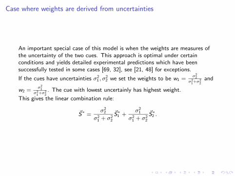
Case where weights are derived from uncertainties

An important special case of this model is when the weights are measures ofthe uncertainty of the two cues. This approach is optimal under certainconditions and yields detailed experimental predictions which have beensuccessfully tested in some cases [69, 32], see [21, 48] for exceptions.

If the cues have uncertainties σ21 , σ

22 we set the weights to be w1 =

σ22

σ21 +σ2

2and

w2 =σ2

1

σ21 +σ2

2. The cue with lowest uncertainly has highest weight.

This gives the linear combination rule:

~S∗ =σ2

2

σ21 + σ2

2

~S∗1 +σ2

1

σ21 + σ2

2

~S∗2 .

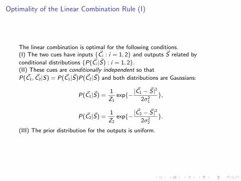
Optimality of the Linear Combination Rule (I)

The linear combination is optimal for the following conditions.(I) The two cues have inputs { ~Ci : i = 1, 2} and outputs ~S related by

conditional distributions {P( ~Ci |~S) : i = 1, 2}.(II) These cues are conditionally independent so that

P( ~C1, ~C2|S) = P( ~C1|~S)P( ~C2|~S) and both distributions are Gaussians:

P( ~C1|~S) =1

Z1exp{−|

~C1 − ~S |2

2σ21

},

P( ~C2|~S) =1

Z2exp{−|

~C2 − ~S |2

2σ22

}.

(III) The prior distribution for the outputs is uniform.

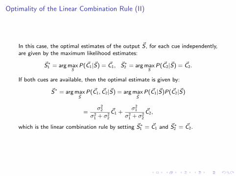
Optimality of the Linear Combination Rule (II)

In this case, the optimal estimates of the output ~S , for each cue independently,are given by the maximum likelihood estimates:

~S∗1 = arg maxS

P( ~C1|~S) = ~C1, ~S∗2 = arg maxS

P( ~C2|~S) = ~C2.

If both cues are available, then the optimal estimate is given by:

~S∗ = arg max~S

P( ~C1, ~C2|~S) = arg max~S

P( ~C1|~S)P( ~C2|~S)

=σ2

2

σ21 + σ2

2

~C1 +σ2

1

σ21 + σ2

2

~C2,

which is the linear combination rule by setting ~S∗1 = ~C1 and ~S∗2 = ~C2.

Optimality of Combination Rule: Illustration

Figure 33: The work of Ernst and Banks shows that cues are sometimes combined byweighted least squares where the weights depend on the variance of the cues. Figureadapted from [32]. The interactive demo (5) illustrates how the cues coupling resultdepends on the means and variances of each cue.

Bayesian Analysis: Weak and Strong Coupling

We now describe more complex models for coupling cues from a Bayesianperspective [22][185] which emphasizes that the uncertainties of the cues aretaken into account and the statistical dependencies between the cue are madeexplicit.Examples of cue coupling, where the cues and independent, are called “weakcoupling” in this framework. In the likelihood functions are independentGaussians and if the priors are uniform, then this reduces to the linearcombination rule.By contrast, “strong coupling” is required if the cues are dependent on eachother.

The priors: avoiding double counting (I)

Models of individual cues typically include prior probabilities about ~S . Forexample, cues for estimating shape or depth assume that the viewed scene ispiecewise smooth. Hence it is typically unrealistic to assume that the priorsP(~S) are uniform.Suppose we have two cues for estimating the shape of a surface which both usethe prior that the surface is spatially smooth. Taking a linear weighted sum ofthe cues will not be optimal, because the prior would be used twice. Priorsintroduce a bias to perception so we want to avoid doubling this bias.This is supported by experimental findings [18] where subjects were asked toestimate the orientation of surfaces using shading cue, texture cues, or bothcombination. If only one cue, shading or texture, was available than subjectsunderestimated the surface orientation. But human estimates were much moreaccurate if both cues were present, inconsistent with double counting priors[185].

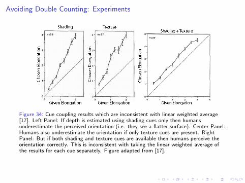
Avoiding Double Counting: Experiments

Figure 34: Cue coupling results which are inconsistent with linear weighted average[17]. Left Panel: If depth is estimated using shading cues only then humansunderestimate the perceived orientation (i.e. they see a flatter surface). Center Panel:Humans also underestimate the orientation if only texture cues are present. RightPanel: But if both shading and texture cues are available then humans perceive theorientation correctly. This is inconsistent with taking the linear weighted average ofthe results for each cue separately. Figure adapted from [17].

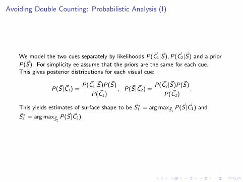
Avoiding Double Counting: Probabilistic Analysis (I)

We model the two cues separately by likelihoods P( ~C1|~S),P( ~C2|~S) and a prior

P(~S). For simplicity ee assume that the priors are the same for each cue.This gives posterior distributions for each visual cue:

P(~S | ~C1) =P( ~C1|~S)P(~S)

P( ~C1), P(~S | ~C2) =

P( ~C2|~S)P(~S)

P( ~C2).

This yields estimates of surface shape to be ~S∗1 = arg max~S1P(~S | ~C1) and

~S∗2 = arg max~S2P(~S | ~C2).

Avoiding Double Counting: Probabilistic Analysis (II)

The optimal way to combine the cues is to estimate ~S from the posteriorprobability P(~S | ~C1, ~C2):

P(~S | ~C1, ~C2) =P( ~C1, ~C2|~S)P(~S)

P( ~C1, ~C2).

If the cues are conditionally independent, P( ~C |~S) = P( ~C1|~S)P( ~C2)|~S), thenthis simplifies to:

P(~S | ~C1, ~C2) =P( ~C1|~S)P( ~C2|~S)P(~S)

P( ~C1, ~C2).

Avoiding Double Counting: Probabilistic Analysis (III)

Coupling the cues, using the model in the previous slide, cannot correspond toa linear weighted sum, which would essentially be using the prior twice (oncefor each cue).

To understand this, suppose the prior is P(~S) = 1Zp

exp{− |~S−~Sp |2

2σ2p}. Then,

setting t1 = 1/σ21 , t2 = 1/σ2

2 , tp = 1/σ2p, the optimal combination is

~S∗ =t1 ~C1+t2 ~C2+tp~Sp

t1+t2+tp, hence the best estimate is a linear weighted combination of

the two cues ~C1, ~C2 and the mean ~Sp of the prior.By contrast, the estimate using each cue individually are given by~S∗1 =

t1 ~C1+tp~Spt1+t2+tp

and ~S∗2 =t2 ~C2+tp~Spt1+t2+tp

.