CUBICAL APPROXIMATION FOR DIRECTED TOPOLOGYsanjeevi/papers/approx.pdf · CUBICAL APPROXIMATION FOR...

CUBICAL APPROXIMATION FOR DIRECTED TOPOLOGY

SANJEEVI KRISHNAN

Abstract. Topological spaces - such as classifying spaces, configuration spaces

and spacetimes - often admit extra directionality. Qualitative invariants on

such directed spaces often are more informative, yet more difficult, to calculatethan classical homotopy invariants because directed spaces rarely decompose

as homotopy colimits of simpler directed spaces. Directed spaces often arise as

geometric realizations of simplicial sets and cubical sets equipped with order-theoretic structure encoding the orientations of simplices and 1-cubes. We

show that, under definitions of weak equivalences appropriate for the directed

setting, geometric realization induces an equivalence between homotopy dia-gram categories of cubical sets and directed spaces and that its right adjoint

satisfies a homotopical analogue of excision. In our directed setting, cubicalsets with structure reminiscent of higher categories serve as analogues of Kan

complexes. Along the way, we prove appropriate simplicial and cubical ap-

proximation theorems and give criteria for two different homotopy relationson directed maps in the literature to coincide.

Contents

1. Background 22. Introduction 23. Conventions 54. Streams 75. Simplicial models 95.1. Simplicial sets 95.2. Subdivisions 105.3. Realizations 126. Cubical models 156.1. Cubical sets 156.2. Subdivisions 166.3. Extensions 186.4. Realizations 197. Triangulations 208. Homotopy 268.1. Streams 268.2. Cubical sets 278.3. Equivalence 299. Conclusion 37Appendix 37

1

2 SANJEEVI KRISHNAN

1. Background

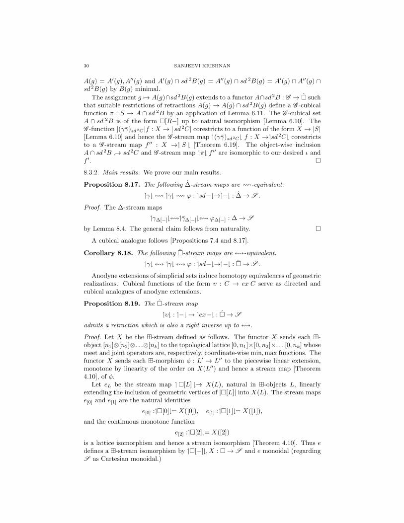
Spaces in nature often come equipped with directionality. Topological examplesof such spaces include spacetimes and classifying spaces of categories. Combina-torial examples of such spaces include higher categories, cubical sets, and simpli-cial sets. Directed geometric realizations translate from the combinatorial to thetopological. Those properties invariant under deformations respecting the tem-poral structure of such spaces can reveal some qualitative features of spacetimes,categories, and computational processes undetectable by classical homotopy types[6, 17, 22]. Examples of such properties include the global orderability of space-time events and the existence of non-determinism in the execution of concurrentprograms [6]. A directed analogue of singular (co)homology [12], constructed interms of appropriate singular cubical sets on directed spaces, should systemize theanalyses of seemingly disparate dynamical processes. However, the literature lacksgeneral tools for computing such invariants. In particular, homotopy extensionproperties, convenient for proving cellular and simplicial approximation theorems,almost never hold for directed maps [Figure 1].

Figure 1. Failure of a homotopy through monotone maps to ex-tend. A directed path on the illustrated square annulus [0, 3]\ [1, 2]is a path monotone in both coordinates. The illustrated dottedhomotopy of maps from {0, 1} to [0, 3]2 \ [1, 2]2 fails to extend to ahomotopy through directed paths from the illustrated solid directedpath.

Current tools in the literature focus on decomposing the structure of directedpaths and undirected homotopies through such directed paths on a directed topo-logical space. For general directed topological spaces, such tools include van Kam-pen Theorems for directed analogues of path-components [7, Proposition 4] anddirected analogues of fundamental groupoids [11, Theorem 3.6]. For directed geo-metric realizations of cubical sets, additional tools include a cellular approximationtheorem for directed paths [5, Theorem 4.1], a cellular approximation theorem forundirected homotopies through directed paths [5, Theorem 5.1], and prod-simplicialapproximations of undirected spaces of directed paths [23, Theorem 3.5]. Exten-sions of such tools for higher dimensional analogues of directed paths are currentlylacking in the literature.

2. Introduction

An equivalence between combinatorial and topological homotopy theories canprovide practical methods for decomposing homotopy types of topological models,in both classical and directed settings. For example, simplicial approximation [3]

CUBICAL APPROXIMATION FOR DIRECTED TOPOLOGY 3

makes the calculation of singular (co)homology groups on compact triangulablespaces tractable. The goal of this paper is to establish an equivalence between di-rected homotopy theories of cubical sets and directed topological spaces. In partic-ular, we formalize the following dictionary between classical and directed homotopytheories.

classical directed

spaces streams (=locally preordered spaces)compact triangulable spaces compact quadrangulable streams

Kan cubical sets cubical sets locally resembling nervesbarycentric subdivision cubical analogue of edgewise subdivision

geometric realization stream realizationhomotopies homotopies defining stream maps

We recall models, both topological and combinatorial, of directed spaces andconstructions between them. A category S of streams [14], spaces equipped withcoherent preorderings of their open subsets, provides topological models. Somenatural examples are spacetimes and connected and compact Hausdorff topologicallattices. A category � of cubical sets [10] provides combinatorial models. The

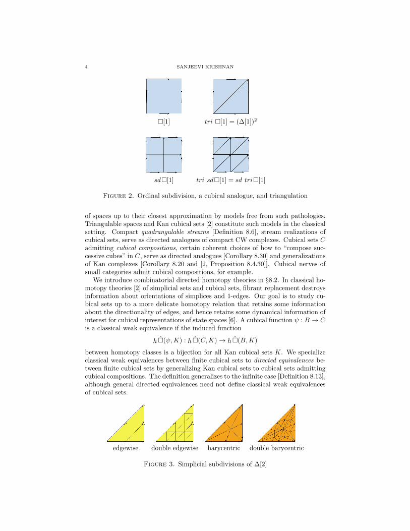
category ∆ of simplicial sets provides models intermediate in rigidity and henceserves as an ideal setting for comparing the formalisms of streams and cubical sets.Stream realization functors �−� [Definitions 5.11 and 6.18], triangulation tri [Def-inition 7.1], edgewise (ordinal) subdivision sd [Figures 2 and 3, [4], and Definition5.7], and a cubical analogue sd [Definition 6.8] relate these three categories in thefollowing commutative diagram [Figure 2 and Propositions 7.4 and 7.5].

�

�−��

sd

��

∆

�−��

sd

S

�

�−�

??

tri

55 ∆

�−�

``

We prove that the functors exhibit convenient properties, which we use in ourproof of the main results. Just as double barycentric simplicial subdivisions factorthrough polyhedral complexes [3], quadruple cubical subdivisions locally factor, in acertain sense [Lemmas 6.10 and 6.12], through representable cubical sets. Triangu-lation and geometric realization both translate rigid models of spaces (cubical sets,simplicial sets) into more flexible models (simplicial sets, topological spaces.) How-ever, the composite of triangulation with its right adjoint - unlike the composite ofgeometric realization with its right adjoint - is cocontinuous [Lemma 7.2]. Streamrealization functors inherit convenient properties from their classical counterparts.

Theorem 5.13. The functor �−� : ∆→ S preserves finite products.

Theorem 6.19. The functor �−� : �→ S sends monics to stream embeddings.

Topological and combinatorial formalisms allow for pathologies irrelevant to ho-motopy theory. In both classical and directed settings, we study the homotopy types

4 SANJEEVI KRISHNAN

�[1] tri �[1] = (∆[1])2

sd�[1] tri sd�[1] = sd tri�[1]

Figure 2. Ordinal subdivision, a cubical analogue, and triangulation

of spaces up to their closest approximation by models free from such pathologies.Triangulable spaces and Kan cubical sets [2] constitute such models in the classicalsetting. Compact quadrangulable streams [Definition 8.6], stream realizations ofcubical sets, serve as directed analogues of compact CW complexes. Cubical sets Cadmitting cubical compositions, certain coherent choices of how to “compose suc-cessive cubes” in C, serve as directed analogues [Corollary 8.30] and generalizationsof Kan complexes [Corollary 8.20 and [2, Proposition 8.4.30]]. Cubical nerves ofsmall categories admit cubical compositions, for example.

We introduce combinatorial directed homotopy theories in §8.2. In classical ho-motopy theories [2] of simplicial sets and cubical sets, fibrant replacement destroysinformation about orientations of simplices and 1-edges. Our goal is to study cu-bical sets up to a more delicate homotopy relation that retains some informationabout the directionality of edges, and hence retains some dynamical information ofinterest for cubical representations of state spaces [6]. A cubical function ψ : B → Cis a classical weak equivalence if the induced function

h �(ψ,K) : h �(C,K)→ h �(B,K)

between homotopy classes is a bijection for all Kan cubical sets K. We specializeclassical weak equivalences between finite cubical sets to directed equivalences be-tween finite cubical sets by generalizing Kan cubical sets to cubical sets admittingcubical compositions. The definition generalizes to the infinite case [Definition 8.13],although general directed equivalences need not define classical weak equivalencesof cubical sets.

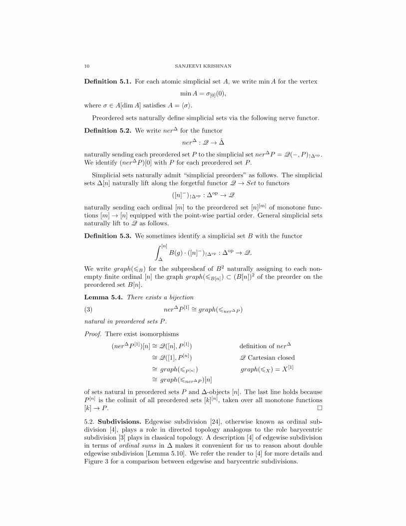
edgewise double edgewise barycentric double barycentric

Figure 3. Simplicial subdivisions of ∆[2]


We introduce a homotopy theory for streams in §8.1. Intuitively, a directedhomotopy of stream maps X → Y should be a stream map I → Y X from theunit interval I equipped with some local preordering to the mapping stream Y X .The literature [6, 11] motivates two distinct homotopy relations, corresponding todifferent choices of stream-theoretic structure on I, on stream maps [Figure 2].The weaker, and more intuitive, of the definitions relates stream maps X → Yclassically homotopic through stream maps. We adopt the stronger [11] of thedefinitions. However, we show that both homotopy relations coincide for the caseX compact and Y quadrangulable [Theorem 8.22], generalizing a result for X adirected unit interval and Y a directed realization of a precubical set [5, Theorem5.6].

A directed equivalence of streams is a stream map f : X → Y inducing bijections

hS (Q, f) : hS (Q,X)→ hS (Q,Y )

of directed homotopy classes of stream maps, for all Q compact quadrangulable[Definition 8.6]. Directed equivalences X → Y between compact quadrangulablestreams are classical homotopy equivalences of underlying spaces. Directed equiv-alences of general quadrangulable streams, however, need not define classical weakequivalences of underlying spaces.

We establish our main results in §8.3, stated in the more general setting of dia-grams of streams and diagrams of cubical sets. We first prove a directed analogue[Theorem 8.23] of classical simplicial approximation up to subdivision and a dualcubical approximation theorem [Corollary 8.24], all for stream maps having com-pact domain. Our proofs, while analogous to classical arguments, require moredelicacy because: simplicial sets and cubical sets do not admit approximations asoriented simplicial complexes and cubical complexes, even up to iterated subdivi-sion; and cubical functions are more difficult to construct than simplicial functions.We then prove a directed analogue of the classical result that maps |B| → |C|admit simplicial approximations B → C for C Kan, at least for the case B finite[Theorem 8.25]. Our main result is the following equivalence. We write h�G and

hS G for the (possibly locally large) localization of diagram categories �G and S G

by appropriate equivariant generalizations of directed equivalences. We sidestepthe question of whether such localizations are locally small; we merely use suchlocalizations as a device for summarizing our main results as follows.

Corollary 8.30. The adjunction �−�a sing induces a categorical equivalence

h�G � hS G

Motivated by our desire to investigate directed (co)homology theories in thefuture, we also prove a homotopical analogue of excision [Corollary 8.31].

3. Conventions

We fix some categorical notation and terminology.

3.0.1. General. We write Set for the category of sets and functions. We write f�Xfor the restriction of a function f : Y → Z to a subset X ⊂ Y . We similarly writeF�A : A → C for the restriction of a functor F : B → C to a subcategory A ⊂ B.We write S · c for the S-indexed coproduct in a category C of distinct copies of a

6 SANJEEVI KRISHNAN

Figure 4. Weak (left) and strong (right) types of directed ho-motopies. The homotopies on both sides are identical up toreparametrization of paths. Only the right homotopy is monotonein the homotopy coordinate, traced by the dotted lines. For com-pact quadrangulable streams, the equivalence relations generatedby weak and strong definitions of directed homotopy are equivalent[Theorem 8.22].

C -object c. Let G denote a small category. For each G , cocomplete category C ,and functor F : G op × G → C , we write∫ g

G

F (g, g)

for the coend [18] of F ; see Appendix §B for details. For each Cartesian closedcategory C , we write −c for the right adjoint to the functor − × c : C → C , foreach C -object c.

3.0.2. Presheaves. Fix a small category G . We write G for the category of presheaves

G op → Set on G and natural transformations between them, call a G -object B a

subpresheaf of a G -object C if B(g) ⊂ C(g) for all G -objects g and B(γ) is a restric-

tion and corestriction of C(γ) for each G -morphism γ, and write G [−] : G → G forthe Yoneda embedding naturally sending a G -object g to the representable presheaf

G [g] = G (−, g) : G op → Set .

For each G -morphism ψ : C → D and subpresheaf B of C, we write

ψ�B : B → D

for the component-wise restriction of ψ to a G -morphism B → D. When a G -objectB and a G -object g are understood, we write 〈σ〉 for the smallest subpresheaf A ⊂ Bsatisfying σ ∈ B(g) and σ∗ for the image of σ under the following natural bijectiondefined by the Yoneda embedding:

B(g) ∼= G (G [g], B)

3.0.3. Supports. We will often talk about the support of a point in a geometricrealization and the carrier of a simplex in a simplicial subdivision. We provide auniform language for such generalized supports. For an object c in a given category,we write b ⊂ c to indicate that b is a subobject of c.

Definition 3.1. Consider a category B closed under intersections of subobjectsand a functor F : B → A preserving monos. For each B-object b and subobject aof the A -object Fb, we write suppF (a, b) for

(1) suppF (a, b) =⋂{b′ | b′ ⊂ b, a ⊂ Fb′},

the unique minimal subobject b′′ ⊂ b such that a ⊂ Fb′′.


We wish to formalize the observation that supports of small objects are small.We recall definitions of connected and projective objects in a general category inAppendix §C. Our motivating examples for connected and projective objects arerepresentable simplicial sets, representable cubical sets, and singleton spaces.

Definition 3.2. An object a in a category C is atomic if there exists an epi

p→ a

in C with p connected and projective.

We give a proof of the following lemma in Appendix §C. Our motivating exam-ples of F in the following lemma are subdivisions, a triangulation operator convert-ing cubical sets into simplicial sets, and functors taking simplicial sets and cubicalsets to the underlying sets of their geometric realizations.

Lemma 3.3. Consider a pair of small categories G1, G2 and functor

F : G1 → G2

preserving coproducts, epis, monos, and intersections of subobjects. For each G1-object b and atomic C2-subobject a ⊂ Fb, suppF (a, b) is the image of a representablepresheaf.

3.0.4. Order theory. We review some order-theoretic terminology in Appendix §A.For each preordered set X, we write 6X for the preorder on X and graph(6X) forits graph, the subset of X ×X consisting of all pairs (x, y) such that x 6X y. Wewrite [n] for the set {0, 1, . . . , n} equipped with its standard total order and [−1]for the empty preordered set. For a(n order-theoretic) lattice L, we write ∨L and∧L for the join and meet operations L2 → L.

Example 3.4. For all natural numbers n and i, j ∈ [n],

i ∧[n] j = min(i, j), i ∨[n] j = max(i, j).

4. Streams

Various formalisms [6, 11, 14] model topological spaces equipped with some com-patible temporal structure. A category S of streams, spaces equipped with localpreorders [14], suffices for our purposes due to the following facts: the category Sis Cartesian closed [14, Theorem 5.13], the forgetful functor from S to the categoryT of compactly generated spaces creates limits and colimits [14, Proposition 5.8],and S naturally contains a category of connected compact Hausdorff topologicallattices as a full subcategory [Theorem 3.9].

Definition 4.1. A circulation 6 on a space X is a function assigning to each opensubset U of X a preorder 6U on U such that for each collection O of open subsetsof X, 6⋃

O is the preorder on⋃O with smallest graph containing

(2)⋃U∈O

graph(6U ).

The circulation 6 on a weak Hausdorff space X is a k-circulation if for each opensubset U ⊂ X and pair x 6U y, there exist compact Hausdorff subspace K ⊂ Uand circulation 6′ on K such that x 6′K y and graph(6′K∩V ) ⊂ graph(6V ) foreach open subset V of X.

8 SANJEEVI KRISHNAN

A circulation is the data of a certain type of “cosheaf.” A k-circulation is acosheaf which is “compactly generated.”

Definition 4.2. A stream X is a weak Hausdorff space equipped with a k-circulationon it, which we often write as 6. A stream map is a continuous function

f : X → Y

from a stream X to a stream Y satisfying f(x) 6U f(y) whenever x 6f−1U y, foreach open subset U of Y . We write T for the category of weak Hausdorff k-spacesand continuous functions, S for the category of streams and stream maps, and Qfor the category of preordered sets and monotone functions.

Just as functions to and from a space induce initial and final topologies, con-tinuous functions to and from streams induce initial and final circulations [14,Proposition 5.8] and [1, Proposition 7.3.8] in a suitable sense.

Proposition 4.3. The forgetful functor S → T is topological.

In particular, the forgetful functor S → T creates limits and colimits.

Proposition 4.4 ([14, Lemma 5.5, Proposition 5.11]). The forgetful functor

S → Q,

sending each stream X to its underlying set equipped with 6X , preserves colimitsand finite products.

Theorem 4.5 ([14, Theorem 5.13]). The category S is Cartesian closed.

An equalizer in S of a pair X ⇒ Y of stream maps is a stream map e : E → Xsuch that e defines an equalizer in T and e is a stream embedding.

Definition 4.6. A stream embedding e is a stream map Y → Z such that for allstream maps f : X → Z satisfying f(X) ⊂ Y , there exists a unique dotted streammap making the following diagram commute.

Xf //

��

Z

Y

e

>>

Stream embeddings define topological embeddings of underlying spaces [Propo-sition 4.3]. Inclusions, from open subspaces equipped with suitable restrictions ofcirculations, are embeddings. However, general stream embeddings are difficultto explicitly characterize. We list some convenient criteria for a map to be anembedding. The following criterion follows from the definition of k-circulations.

Lemma 4.7. For a stream map f : X → Y , the following are equivalent.

(1) The map f is a stream embedding.(2) For each embedding k : K → X from a compact Hausdorff stream K, fk is

a stream embedding.

The following criterion, straightforward to verify, is analogous to the statementthat a sheaf F on a space X is the pullback of a sheaf G on a space Y along aninclusion i : X ↪→ Y if for each open subset U of X, FU is the colimit, taken overall open subsets V of Y containing U , of objects of the form GV .


Lemma 4.8. A stream map f : X → Y is a stream embedding if

graph(6XU ) = U2 ∩⋂

V ∈BU

graph(6YV ),

for each open subset U of X, where BY is a basis of open neighborhoods in Y of U ,6X and 6Y are the respective circulations on X and Y , and f defines an inclusionof a subspace.

A topological lattice is a(n order theoretic) lattice L topologized so that its joinand meet operations ∨L,∧L : L2 → L are jointly continuous.

Definition 4.9. We write ~I for the unit interval

I = [0, 1],

regarded as a topological lattice whose join and meet operations are respectivelydefined by maxima and minima.

We can regard a category of connected and compact Hausdorff topological lat-tices as a full subcategory of S [14, Propositions 4.7, 5.4, 5.11], [21, Proposition 1,Proposition 2, and Theorem 5], [8, Proposition VI-5.12 (i)], [8, Proposition VI-5.15].

Theorem 4.10. There exists a full dotted embedding making the diagram

P //

�� !!

Q

T S ,oo

OO

where P is the category of compact Hausdorff connected topological lattices andmonotone maps between them and the solid arrows are forgetful functors, commute.

We henceforth regard connected compact Hausdorff topological lattices, such as~I, as streams.

5. Simplicial models

Simplicial sets serve as technically convenient models of directed spaces. Firstly,edgewise (ordinal) subdivision, the subdivision appropriate for preserving the di-rectionality encoded in simplicial orientations, is simple to define [Definition 5.7]and hence straightforward to study [Lemma 5.10]. Secondly, the graphs of natu-ral preorders 6�B� on geometric realizations |B| of simplicial sets B admit concisedescriptions in terms of the structure of B itself [Lemma 5.12].

5.1. Simplicial sets. We write ∆ for the category of finite non-empty ordinals

[n] = {0 6[n] 1 6[n] · · · 6[n] n}, n = 0, 1, . . .

and monotone functions between them. Simplicial sets are ∆-objects and simplicialfunctions are ∆-morphisms. We refer the reader to [20] for the theory of simpli-cial sets. The representable simplicial sets ∆[n] = ∆(−, [n]) model combinatorialsimplices. The vertices of a simplicial set B are the elements of B([0]). For eachsimplicial set B, we write dimB for the infimum of all natural numbers n such thatthe natural simplicial function B[n] · [n]→ B is epi. For each atomic simplicial setA, there exists a unique σ ∈ A[dimA] such that A = 〈σ〉. Atomic simplicial sets arethose simplicial sets of the form 〈σ〉. Every atomic simplicial set has a “minimumvertex,” defined as follows.

10 SANJEEVI KRISHNAN

Definition 5.1. For each atomic simplicial set A, we write minA for the vertex

minA = σ[0](0),

where σ ∈ A[dimA] satisfies A = 〈σ〉.

Preordered sets naturally define simplicial sets via the following nerve functor.

Definition 5.2. We write ner∆ for the functor

ner∆ : Q → ∆

naturally sending each preordered set P to the simplicial set ner∆P = Q(−, P )�∆op .We identify (ner∆P )[0] with P for each preordered set P .

Simplicial sets naturally admit “simplicial preorders” as follows. The simplicialsets ∆[n] naturally lift along the forgetful functor Q → Set to functors

([n]−)�∆op : ∆op → Q

naturally sending each ordinal [m] to the preordered set [n][m] of monotone func-tions [m]→ [n] equipped with the point-wise partial order. General simplicial setsnaturally lift to Q as follows.

Definition 5.3. We sometimes identify a simplicial set B with the functor∫ [n]

∆

B(g) · ([n]−)�∆op : ∆op → Q.

We write graph(6B) for the subpresheaf of B2 naturally assigning to each non-empty finite ordinal [n] the graph graph(6B[n]) ⊂ (B[n])2 of the preorder on thepreordered set B[n].

Lemma 5.4. There exists a bijection

(3) ner∆P [1] ∼= graph(6ner∆P )

natural in preordered sets P .

Proof. There exist isomorphisms

(ner∆P [1])[n] ∼= Q([n], P [1]) definition of ner∆

∼= Q([1], P [n]) Q Cartesian closed

∼= graph(6P [n]) graph(6X) = X [1]

∼= graph(6ner∆P )[n]

of sets natural in preordered sets P and ∆-objects [n]. The last line holds becauseP [n] is the colimit of all preordered sets [k][n], taken over all monotone functions[k]→ P . �

5.2. Subdivisions. Edgewise subdivision [24], otherwise known as ordinal sub-division [4], plays a role in directed topology analogous to the role barycentricsubdivision [3] plays in classical topology. A description [4] of edgewise subdivisionin terms of ordinal sums in ∆ makes it convenient for us to reason about doubleedgewise subdivision [Lemma 5.10]. We refer the reader to [4] for more details andFigure 3 for a comparison between edgewise and barycentric subdivisions.


Definition 5.5. We write ⊕ for the tensor, sending pairs [m], [n] of finite ordinalsto [m+ n+ 1] and pairs φ′ : [m′]→ [n′], φ′′ : [m′′]→ [n′′] of monotone functions tothe monotone function (φ′ ⊕ φ′′) : [m′ +m′′ + 1]→ [n′ + n′′ + 1] defined by

(φ′ ⊕ φ′′)(k) =

{φ′(k), k = 0, 1, . . . ,m′

n′ + 1 + φ′′(k −m′ − 1), k = m′ + 1,m′ + 2, . . . ,m′ +m′′ + 1,

on the category of finite ordinals [−1] = ∅, [0] = {0}, [1] = {0 < 1}, [2] = {0 < 1 <2}, . . . and monotone functions between them.

In particular, the empty set [−1] = ∅ is the unit of the tensor ⊕. We can thusdefine natural monotone functions [n]→ [n]⊕ [n] as follows.

Definition 5.6. We write γ∆[n], γ

∆[n] for the monotone functions

γ∆[n] = [n]⊕ ([−1]→ [n]), γ∆

[n] = ([−1]→ [n])⊕ [n] : [n]→ [n]⊕ [n],

natural in finite ordinals [n].

In other words, γ∆[n] and γ∆

[n] are the monotone functions [n] → [2n + 1] respec-

tively defined by inclusion and addition by n+ 1.

Definition 5.7. We write sd for the functor ∆→ ∆ induced from the functor

(−)⊕2 : ∆→ ∆.

Natural monotone functions [n] → [n] ⊕ [n] induce natural simplicial functionssdB → B, defined as follows.

Definition 5.8. We write γ, γ for the natural transformations

γ, γ : sd→ id∆ : ∆→ ∆

respectively induced from the natural monotone functions γ∆[n], γ

∆[n] : [n]→ [n]⊕ [n].

The functor sd , and hence sd 2, are left and right adjoints [4, §4] and hencesd 2 preserves monos, intersections of subobjects, and colimits. Thus we can con-struct supp sd2(B,C) ⊂ C [Definition 3.1] for simplicial sets C and subpresheavesB ⊂ sd 2C. The following observations about double edgewise subdivisions of thestandard 1-simplex ∆[1] later adapt to the cubical setting [Lemmas 6.10 and 6.12].

Lemma 5.9. For all atomic subpresheaves A ⊂ sd2∆[1] and v ∈ A[0],

(γγ)∆[1](A) ⊂ suppsd2(〈v〉,∆[1]).

Proof. Each v ∈ A[0] ⊂ ∆([0]⊕4, [1]) is a monotone function

v : [3]→ [1]

The case v : [3]→ [1] non-constant holds because

suppsd2(〈v〉,∆[1]) = ∆[1].

Consider the case v a constant function. Let n = dimA and σ be the monotonefunction [n]⊕ [n]⊕ [n]⊕ [n]→ [1], an element in (sd 2∆[1])[n], such that A = 〈σ〉.There exists a k ∈ [n] such that v(0) = σ(k), v(1) = σ(k+n+1), v(2) = σ(k+2n+2)and v(3) = σ(k + 3n+ 3) because v ∈ 〈σ〉[0]. Therefore

v(0) = σ(k) 6[1] σ(k + 1) 6[1] · · · 6[1] σ(k + 2n+ 2) = v(0),


hence σ(n+ 1 + i) = v(0) for all i ∈ [n], hence

(((γγ)∆[1])[n]σ)(i) = (σ(γ∆[n] ⊕ γ

∆[n])(γ

∆[n])(i))

= σ(n+ 1 + i)

= v(0)

for all i = 0, 1, . . . , n. Thus ((γγ)∆[1])[n]σ is a constant function [n] → [1] taking

the value v(0) and hence (γγ)∆[1]A = 〈v(0)〉 = suppsd2(〈v〉, sd2∆[1]). �

Lemma 5.10. For each atomic subpresheaf A ⊂ sd 2∆[1], there exists a uniqueminimal subpresheaf B ⊂ ∆[1] such that A ∩ sd2B 6= ∅. Moreover, the diagram

(4) A //

π

��

sd2∆[1](γγ)∆[1] // ∆[1]

A ∩ sd2B // sd2∆[1](γγ)∆[1]

// ∆[1],

where π : A → A ∩ sd 2B is the unique retraction of A onto A ∩ sd 2B and theunlabelled solid arrows are inclusions, commutes.

Proof. In the case A ∩ sd 2〈0〉 = A ∩ sd 2〈1〉 = ∅, then ∆[1] is the unique choiceof subpresheaf B ⊂ ∆[1] such that A ∩ sd 2B 6= ∅ and hence id∆[1] is the uniquechoice of retraction π making (4) commute.

It therefore remains to consider the case A∩sd2〈0〉 6= ∅ and the case A∩sd2〈1〉 6=∅ because the only non-empty proper subpresheaves of ∆[1] are 〈0〉 and 〈1〉. Weconsider the case A ∩ sd2〈0〉 6= ∅, the other case following similarly. Observe

(5) (γγ)∆[1]A ⊂ 〈0〉[Lemma 5.9.] In particular, A∩ sd2〈1〉 = ∅ because (γγ)〈1〉(sd

2〈1〉) ⊂ 〈1〉 [Lemma

5.9]. Thus 〈0〉 is the minimal subpresheaf B′ of B such that A ∩ sd 2B′ 6= ∅.Moreover, the terminal simplicial function π : ∆[1]→ ∆[0] makes (4) commute by(5). �

5.3. Realizations. Classical geometric realization is the unique functor

| − | : ∆→ T

preserving colimits, assigning to each simplicial set ∆[n] the topological n-simplex,and assigning to each simplicial function of the form ∆[φ : [m]→ [n]] : ∆[m]→ ∆[n]the linear map |∆[m]| → |∆[n]| sending each point with kth barycentric coordinate1 to the point with φ(k)th barycentric coordinate 1. For each simplicial set B andv ∈ B[0], we write |v| for the image of |v∗| : |∆[0]| → |B| and call |v| a geometricvertex in |B|.

Definition 5.11. We write �−� for the unique functor

�−� : ∆→ S

naturally preserving colimits, assigning to each simplicial set ∆[n] the space |∆[n]|equipped with respective lattice join and meet operations

|ner∆ ∨[n] |, |ner∆ ∧[n] | : |ner∆[n]|2 → |ner∆[n]|,and assigning to each simplicial function ψ : B → C the stream map �B�→�C �defined by |ψ| : |B| → |C|.


We can directly relate the circulation of a stream realization �B � with thesimplicial structure of B as follows.

Lemma 5.12. There exists a bijection of underlying sets

graph(6�B�) ∼= | graph(6B)|natural in simplicial sets B.

Proof. For the case B = ∆[n], graph(6�∆[n]�) = · · ·

= lim(|ner∆ ∧[n] | × |ner∆ ∨[n] |, id|ner∆[n]|2 : |ner∆[n]|2 → |ner∆[n]|2)

= |ner∆ lim(∧[n] × ∨[n], id[n]2 : [n]2 → [n]2)|

= |ner∆[n][1]|= | graph(6∆[n])|.

Among the above lines, the first and third follow from Lemma A.6, the secondfollows from |ner∆ − | finitely continuous, and the last follows from Lemma 5.4.The general case follows because the forgetful functor S → Q preserves colimits[Proposition 4.4]. �

Theorem 5.13. The functor �−� : ∆→ S preserves finite products.

Proof. There exists a bijection graph(6�ner∆L�) = · · ·= | graph(6ner∆L)|

= |ner∆L[1]|= |ner∆ lim(∧L × ∨L, idL2 : L2 → L2)|= lim(|ner∆ ∧L | × |ner∆ ∨L |, id|ner∆L|2 : |ner∆L|2 → |ner∆L|2)

natural in lattices L, and hence the underlying preordered set of �ner∆L � is alattice natural in lattices L. Among the above lines, the first follows from Lemma5.12, the second follows from Lemma 5.4, the third follows from Lemma A.6, andthe last follows from |ner∆ − | finitely continuous.

The universal stream map �A×B� ∼= �A� × �B�, a homeomorphism of underly-ing spaces because |− | preserves finite products, thus defines a bijective lattice ho-momorphism, and hence isomorphism, of underlying lattices for the case A = ∆[m],B = ∆[n], hence a stream isomorphism for the case A = ∆[m], B = ∆[n] [Theorem4.10], and hence a stream isomorphism for the general case because finite products

commute with colimits in ∆ and S [Theorem 4.5]. �

We can recover some information about the orientations of a simplicial set Bfrom relations of the form x 6�B� y as follows. Recall our definition [Definition 5.1]of the minimum minA of an atomic simplicial set A.

Lemma 5.14. For all preordered sets P and pairs x 6�ner∆P� y,

min supp|−|({x}, ner∆P ) 6P min supp|−|({y}, ner∆P ).

Proof. The underlying preordered set of �ner∆P� is the colimit, over all monotonefunctions [k] → P , of underlying preordered sets of topological lattices �∆[k]� be-

cause �−�: ∆→ S and the forgetful functor S → Q are cocontinuous [Proposition4.4].


Therefore it suffices to consider the case P = [n]. Let ti be the ith barycentriccoordinate of t ∈�∆[n]� for each i ∈ [n]. Then

n∑i=0

yi(i) = y definition of ti’s

= x ∨�∆[n]� y x 6�ner∆P� y

=

(n∑i=0

xi(i)

)∨�∆[n]�

n∑j=0

yj(j)

definition of ti’s

=∑i,j∈[n]

(xiyj)(max(i, j)) linearity of ∨�∆[n]�.

We conclude that for each j = 0, 1, ..., n,

yj =∑

max(i,j)=j

xiyj =

j∑i=0

xiyj

and hence yj 6= 0 implies the existence of some i = 0, 1, ..., j such that xi 6= 0. Thus

min �supp|−|({x}, ner∆P )� = min{i | xi 6= 0}6[n] min{j | yj 6= 0}= min �supp|−|({y}, ner∆P )� .

�

Edgewise subdivisions respect geometric realizations as follows.

Definition 5.15. We write ϕ∆[n] for the piecewise linear map

ϕ∆[n] : | sd∆[n]| ∼= |∆[n]| = ∇[n],

natural in non-empty finite ordinals [n], characterized by the rule

|φ| 7→ 1/2|φ(0)|+ 1/2|φ(1)|, φ ∈ (sd∆[n])[0] = ∆([0]⊕ [0], [n]).

These maps ϕ∆[n], prism decompositions in the parlance of [19], define homeo-morphisms [19]. The restriction of the function ϕ∆[n] : | sd∆[n]| → |∆[n]| to thegeometric vertices Q([0]⊕ [0], [n]) of | sd∆[n]| is a lattice homomorphism

[n][0]⊕[0] →�∆[n]�

natural in ∆-objects [n] by ∨�∆[n]�,∧�∆[n]� : |∆[n|2 → |∆[n]| linear. Thus

ϕ∆[n] :�∆[n]�→�∆[n]�,

the linear extension of a lattice homomorphism, defines a lattice isomorphism by∧�∆[n]� and ∨�∆[n]� linear, and hence stream isomorphism [Theorem 4.10], naturalin ordinals [n]. We can thus make the following definition.

Definition 5.16. We abuse notation and write ϕB for the isomorphism

ϕB : �sdB� ∼= �B�,

of streams natural in simplicial sets B, defined by prism decompositions for thecase B representable.


6. Cubical models

Cubical sets are combinatorial and economical models of directed spaces [6, 9].Cubical subdivisions appropriate for directed topology, unlike edgewise subdivisionsof simplicial sets, mimic properties of simplicial barycentric subdivision [Lemmas6.10 and 6.12] that make classical simplicial approximation techniques adaptableto the directed setting.

6.1. Cubical sets. We refer the reader to [10] for basic cubical theory. Definitionsof the box category, over which cubical sets are defined as presheaves, are notstandard [10]. We adopt the simplest of the definitions.

Definition 6.1. We write �1 for the full subcategory of Q containing the ordinals[0] and [1]. Let � be the smallest subcategory of Q containing �1 and closed underbinary Q-products. We write ⊗ for the tensor on � defined by binary Q-products.

To avoid confusion between tensor and Cartesian products in �, we write

[0], [1], [1]⊗2, [1]⊗3, . . . .

for the �-objects. We will often use the following characterization [[10, Theorem4.2] and [2, Proposition 8.4.6]] of � as the free monoidal category generated by�1, in the following sense, without comment. For each monoidal category C andfunctor F : �1 → C of underlying categories sending [0] to the unit of C , thereexists a unique dotted monoidal functor, up to natural isomorphism, making thefollowing diagram, in which the vertical arrow is inclusion, commute.

�1F //

��

C

�,

>>

Injective �-morphisms are uniquely determined by where they send extrema.A proof of the following lemma follows from a straightforward verification for �1-morphisms and induction.

Lemma 6.2. There exists a unique injective �-morphism of the form

[1]⊗m → [1]⊗n

sending (0, · · · , 0) to ε′ and (1, · · · , 1) to ε′′, for each n = 0, 1, . . . and m =0, 1, . . . , n, and ε′ 6[1]⊗n ε

′′.

We regard � as a monoidal category whose tensor ⊗ cocontinuously extends thetensor on � along the Yoneda embedding �[−] : � ↪→ �. We can regard eachtensor product B ⊗ C as a subpresheaf of the Cartesian product B × C. Cubicalsets are �-objects and cubical functions are �-morphisms. We write the cubicalset represented by the box object [1]⊗n as �[1]⊗n. The vertices of a cubical set Bare the elements of B([0]). We will sometimes abuse notation and identify a vertexv of a cubical set B with the subpresheaf 〈v〉 of B. For each cubical set B, wewrite dimB for the infimum of all natural numbers n such that the natural cubicalfunction B[n] · [1]⊗n → B is epi. For each atomic cubical set A, there exists aunique σ ∈ A[1]⊗ dimA such that A = 〈σ〉. Atomic cubical sets, analogous to cellsin a CW complex, admit combinatorial boundaries defined as follows.


Definition 6.3. For each atomic cubical set A, we write

∂A

for the unique maximal proper subpresheaf of A.

Generalizing the quotient Y/X of a set Y by a subset X of Y , we write C/Bfor the object-wise quotient of a cubical set C by a subpresheaf B of C. For eachatomic cubical set A, the unique epi �[1]⊗ dimA → A passes to an isomorphism

�[1]⊗ dimA/∂�[1]⊗ dimA ∼= A/∂A.

Each subpresheaf B of a cubical set C admits a combinatorial analogue of aclosed neighborhood in C, defined as follows.

Definition 6.4. For each cubical set C and subpresheaf B ⊂ C, we write

StarCB

for the union of all atomic subpresheaves of C intersecting B.

6.2. Subdivisions. We construct cubical analogues of edgewise subdivisions. Tostart, we extend the category � of abstract hypercubes to a category � that alsomodels abstract subdivided hypercubes.

Definition 6.5. We write � for the smallest sub-monoidal category of the Carte-sian monoidal category Q containing all monotone functions between [0], [1], [2]except the function [1]→ [2] sending i to 2i. We write ⊗ for the tensor on �. Weabuse notation and also write �[−] for the functor

�→ �naturally sending each �-object L to the cubical set �(−, L)��op : �op → Set.

Context will make clear whether �[−] refers to the Yoneda embedding � → �or its extension � → �. A functor sd : � → � describes the subdivision of anabstract cube as follows.

Definition 6.6. We write sd for the unique monoidal functor

sd : �→ �sending each �1-object [n] to [2n] and each �1-morphism δ : [0] → [1] to the�-morphism [0]→ [2] sending 0 to 2δ(0).

Natural �-morphisms [2]⊗n → [1]⊗n model cubical functions from subdividedhypercubes to ordinary hypercubes.

Definition 6.7. We write γ�[1], γ�[1] for the monotone functions

γ�[1] = max(1,−)− 1, γ�[1] = min(−, 1) : [2]→ [1].

More generally, we write γ�, γ� for the unique monoidal natural transformationssd→ (id�)�� having the above [1]-components.

We extend our subdivision operation from abstract hypercubes to more generalcubical sets.

Definition 6.8. We write sd for the unique cocontinuous monoidal functor

sd : �→ �extending �[−] ◦ sd : �→ � along �[−] : �→ �.


Context will make clear whether sd refers to simplicial or cubical subdivision.

Definition 6.9. We write γ, γ for the natural transformations

sd→ id� : �→ �

induced from the respective natural transformations γ�, γ� : sd→ (id�)��.

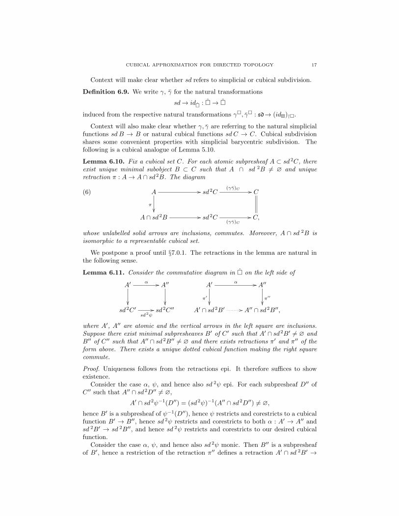
Context will also make clear whether γ, γ are referring to the natural simplicialfunctions sd B → B or natural cubical functions sd C → C. Cubical subdivisionshares some convenient properties with simplicial barycentric subdivision. Thefollowing is a cubical analogue of Lemma 5.10.

Lemma 6.10. Fix a cubical set C. For each atomic subpresheaf A ⊂ sd 2C, thereexist unique minimal subobject B ⊂ C such that A ∩ sd 2B 6= ∅ and uniqueretraction π : A→ A ∩ sd2B. The diagram

(6) A //

π

��

sd2C(γγ)C // C

A ∩ sd2B // sd2C(γγ)C

// C,

whose unlabelled solid arrows are inclusions, commutes. Moreover, A ∩ sd 2B isisomorphic to a representable cubical set.

We postpone a proof until §7.0.1. The retractions in the lemma are natural inthe following sense.

Lemma 6.11. Consider the commutative diagram in � on the left side of

A′α //

��

A′′

��

A′α //

π′

��

A′′

π′′

��sd2C ′

sd2ψ

// sd2C ′′ A′ ∩ sd2B′ // A′′ ∩ sd2B′′,

where A′, A′′ are atomic and the vertical arrows in the left square are inclusions.Suppose there exist minimal subpresheaves B′ of C ′ such that A′ ∩ sd2B′ 6= ∅ andB′′ of C ′′ such that A′′ ∩ sd 2B′′ 6= ∅ and there exists retractions π′ and π′′ of theform above. There exists a unique dotted cubical function making the right squarecommute.

Proof. Uniqueness follows from the retractions epi. It therefore suffices to showexistence.

Consider the case α, ψ, and hence also sd 2ψ epi. For each subpresheaf D′′ ofC ′′ such that A′′ ∩ sd2D′′ 6= ∅,

A′ ∩ sd2ψ−1(D′′) = (sd2ψ)−1(A′′ ∩ sd2D′′) 6= ∅,hence B′ is a subpresheaf of ψ−1(D′′), hence ψ restricts and corestricts to a cubicalfunction B′ → B′′, hence sd 2ψ restricts and corestricts to both α : A′ → A′′ andsd 2B′ → sd 2B′′, and hence sd 2ψ restricts and corestricts to our desired cubicalfunction.

Consider the case α, ψ, and hence also sd 2ψ monic. Then B′′ is a subpresheafof B′, hence a restriction of the retraction π′′ defines a retraction A′ ∩ sd 2B′ →


A′′ ∩ sd 2B′′ onto its image making the right square commute because α, π′′, andhence π′′α are retractions onto their images and retractions of atomic cubical setsare unique.

The general case follows because every cubical function naturally factors as thecomposite of an epi followed by a monic. �

The following is a cubical analogue of Lemma 5.9.

Lemma 6.12. For all cubical sets C and v ∈ (sd2C)[0],

(γγ)C Star sd2C〈v〉 ⊂ suppsd2(〈v〉, C).

We postpone a proof until §7.0.1.

6.3. Extensions. Unlike the right adjoint to simplicial barycentric subdivision, theright adjoint to cubical subdivision sd does not preserve classical weak homotopytype, much less a more refined analogue [Definition 8.13] of weak type for thedirected setting. We modify the right adjoint to sd in order to obtain a directedand cubical analogue of the right adjoint Ex to simplicial barycentric subdivision.

Definition 6.13. We write ex for the functor

ex : �→ �naturally assigning to each cubical set C the cubical set

∫ L� �(�[L], C) · ner�L.

We define natural cubical functions

υB : B → exB, ζB : B → exsdB,

by the following propositions.

Proposition 6.14. There exists a unique natural transformation υ of the form

(7) υ : id� → ex : �→ �.

Proof. Inclusions � ↪→ Q and � ↪→ � induce the cubical function

B =

∫ [1]⊗n

��(�[1]⊗n, B) ·�[1]⊗n →

∫ L

��(�[L], B) · ner�L = exB

natural in cubical sets B. Hence existence follows.The �[0]-component of a natural transformation (7) is the unique terminal cu-

bical function �[0]→ ex�[0] = �[0] and hence each �[1]⊗n-component �[1]⊗n →ex�[1]⊗n = ner�[1]⊗n is uniquely determined because it is determined on vertices.Uniqueness follows from naturality. �

Proposition 6.15. There exists a unique natural transformation ζ of the form

(8) ζ : id� → exsd : �→ �.

Proof. The cubical functions

�[1]⊗n → exsd�[1]⊗n = ex�[2]⊗n = ner�[2]⊗n,

naturally sending each �-morphism of the form φ : [1]⊗m → [1]⊗n to the monotonefunction [1]⊗m → [2]⊗n defined by i 7→ 2φ(i), induce a cubical function B → exsdBnatural in cubical sets B. Hence existence follows.

The �[0]-component of a natural transformation (8) is the unique terminalcubical function �[0] → ex sd �[0] = �[0] and hence each �[1]⊗n-component


�[1]⊗n → ner�[2]⊗n of a natural transformation (8) is uniquely determined be-cause it is determined on vertices. Uniqueness follows from naturality. �

Generalizing n-fold composites ex n : � → � of the functor ex : � → �, weabuse notation and write ex∞ for the functor � → � naturally assigning to eachcubical set B the colimit of the diagram

BυB−−→ exB

υexB−−−→ · · ·

6.4. Realizations. Geometric realization of cubical sets is the unique functor

| − | : �→ T

sending �[0] to {0}, �[1] to the unit interval I, each �-morphism �[δ : [0]→ [1]] :�[0] → �[1] to the map {0} → I defined by the �-morphism δ : [0] → [1], finitetensor products to binary Cartesian products, and colimits to colimits. We defineopen stars of geometric vertices as follows.

Definition 6.16. For each cubical set C and subpresheaf B ⊂ C, we write

starCB

for the topological interior in |C| of the subset |Star CB| ⊂ |C| and call star CBthe open star of B (in C).

Example 6.17. For each cubical set B, the set

{starB〈v〉}v∈B[0]

is an open cover of |B|.

We abuse notation and write {0} for the singleton space equipped with theunique possible circulation on it.

Definition 6.18. We abuse notation and also write �−� for the unique functor

�− � : �→ S

sending �[0] to {0}, �[1] to ~I, each �-morphism �[δ : [0] → [1]] : �[0] → �[1]

to the stream map {0} → ~I defined by the �-morphism δ : [0] → [1], finite tensorproducts to binary Cartesian products, and colimits to colimits.

We can henceforth identify the geometric realization |B| of a cubical set B withthe underlying space of the stream �B � because the forgetful functor S → Tpreserves colimits and Cartesian products [Proposition 4.3]. In our proof of cubicalapproximation, we will need to say that a stream map f :�B�→�D� whose underlyingfunction corestricts to a subset of the form |C| ⊂ |D| corestricts to a stream map�B�→�C�. In order to do so, we need the following observation.

Theorem 6.19. The functor �−� : �→ S sends monics to stream embeddings.

We give a proof at the end of §7.


7. Triangulations

We would like to relate statements about simplicial sets to statements aboutcubical sets. In order to do so, we need to study properties of triangulation, afunctor tri : �→ ∆ decomposing each abstract n-cube into n! simplices [Figure 2].

Definition 7.1. We write tri for the unique cocontinuous functor

tri : �→ ∆

naturally assigning to each cubical set �[1]⊗n the simplicial set ner∆[1]⊗n. We

write qua for the right adjoint ∆→ � to tri.

Triangulation tri restricts and corestricts to an isomorphism between full sub-categories of cubical sets and simplicial sets having dimensions 0 and 1 becausesuch cubical sets and simplicial sets are determined by their restrictions to �op

1 andtri does not affect such restrictions. The functor tri is cocontinuous because it is aleft adjoint. Less formally, qua◦ tri is also cocontinuous.

Lemma 7.2. The composite qua◦ tri : �→ � is cocontinuous.

Proof. Let ηB be the cubical function

(9) ηB :

∫ [1]⊗n

�B([1]⊗n) · qua(tri �[1]⊗n)→ qua(triB)

natural in cubical sets B. Fix a cubical set B and natural number m. It suffices toshow that (ηB)[1]⊗m , injective because qua◦ tri preserves monics, is also surjective.For then η defines a natural isomorphism from a cocontinuous functor to qua◦ tri :�→ �.

Consider a simplicial function σ : tri �[1]⊗m → tri B. Consider a natu-ral number a and monotone function α : [a] → [1]⊗m preserving extrema. Thesubpresheaf supp tri(σ(ner∆α)(∆[a]), B) of B is atomic [Lemma 3.3] and hencethere exist minimal natural number nα and unique θα ∈ B([1]⊗nα) such thatsupp tri(σ(ner∆α)(∆[a]), B) = 〈θα〉 [Lemma 3.3]. There exists a dotted monotonefunction λα : [a]→ [1]⊗nα such that the top trapezoid in the diagram

∆[a]ner∆λα //

ner∆φ

��

ner∆α

%%

tri�[1]⊗nα

tri (θα)∗

yytri�[δφ]

��

tri�[1]⊗m σ // triB

∆[b]ner∆λβ

//

ner∆β

99

tri�[1]⊗nβ

tri (θβ)∗

ee

commutes by ∆[a] projective and ner∆ full. The isomorphism

�[1]⊗nα/∂�[1]⊗nα ∼= θ∗(�[1]⊗nα)/∂θ∗(�[1]⊗nα)

induces an isomorphism

tri�[1]⊗nα/ tri∂�[1]⊗nα ∼= triθ∗(�[1]⊗nα)/ tri∂θ∗(�[1]⊗nα)


by tri cocontinuous and hence (tri (θα)∗)[a] : (tri �[1]⊗nα)[a] → (tri B)[a] is

injective on (tri �[1]⊗nα)[a] \ (tri ∂�[1]⊗nα)[a]. The function λα preserves ex-trema by minimality of nα [Lemma 6.2], hence λα /∈ (tri ∂�[1]⊗nα)[a], hence thechoice of λα is unique by the function (tri (θα)∗)[a] injective on (tri�[1]⊗nα)[a] \(tri∂�[1]⊗nα)[a].

We claim that our choices of nα and θα are independent of our choice of a and α.To check our claim, consider extrema-preserving monotone functions β : [b]→ [1]⊗n

and φ : [a] → [b] such that the left triangle commutes. We have shown that thereexists a unique monotone function λβ preserving extrema and making the bottomtrapezoid commute. There exists a �-morphism δφ such that the right trianglecommutes because �[1]⊗nα is projective and the image of (θα)∗ lies in the image of(θβ)∗. The function δφ preserves extrema because the outer square commutes andλα, φ, λβ preserve extrema. The function δφ is injective by minimality of nα. Thusδφ = id�[1]⊗nα [Lemma 6.2].

Let τ denote a monotone function from a non-empty ordinal to [1]⊗m preservingextrema. We have shown that all nτ ’s coincide and all θτ ’s coincide. Thus we canrespectively define N(σ) and Θ(σ) to be nτ and θτ for any and hence all choices ofτ . The λτ ’s hence induce a simplicial function Σ(σ) : tri�[1]⊗m → tri�[1]⊗N(σ),well-defined by the uniquenesses of the λτ ’s, such that (tri Θ(σ)∗) ◦ Σ(σ) = σ.Thus the preimage of σ under (ηB)[1]⊗n is non-empty. �

Lemma 7.3. There exists an isomorphism

qua(triB) ∼=∫ [1]⊗n

�B([1]⊗n) · ner�[1]⊗n

natural in cubical sets B.

Proof. There exist isomorphisms

qua(tri�[1]⊗n) = qua(ner∆[1]⊗n) = ner�[1]⊗n

natural in �-objects [1]⊗n. The claim then follows by qua◦ tri cocontinuous [Lemma7.2]. �

Triangulation relates our different subdivisions and hence justifies our abuse innotation for sd, γ, and γ.

Proposition 7.4. There exists a dotted natural isomorphism making the diagram

(10) tri tri◦ sd

��

tri γ

%%

tri γoo

sd◦ triγ tri

//γ tri

ee

tri

commute.

Proof. The solid functions in the diagram

(11) �1([m], [n]) �([m], sd [n])

α[m][n]

��

�(id[m],γ�[n])

))

�(id[m],γ�[n])oo

∆([m]⊕2, [n])∆(γ∆

[m],id[n])

//∆(γ∆

[m],id[n])

ii

�1([m], [n]),


describe the [m]-components of the �[n]-components of the solid natural transfor-mations in (10) for the case m,n ∈ {0, 1}. It suffices to construct a bijection α[m][n],natural in �1-objects [m] and [n], making (11) commute. For then the requisitecubical isomorphism ηB , natural in cubical sets B, in (10) would exist for the caseB = �[n] for �1-objects [n], hence for the case B representable because all functors

and natural transformations in (10) are monoidal (where we take ∆ to be Cartesianmonoidal), and hence for the general case by naturality.

Let α[m][n] and β([m],[n]) be the functions

α[m][n] : �([m], sd [n])� ∆([m]⊕2, [n]) : β([m],[n]),

natural in �1-objects [m] and [n], defined by

α[m][n](φ)(i) =

{(γ�[n]φ)(i), i ∈ {0, 1, . . . ,m}(γ�[n]φ)(i−m− 1), i ∈ {m+ 1,m+ 2, . . . , 2m+ 1}

β([m],[n])(φ)(j) = φγ∆[m](j) + φγ∆

[m](j), j = 0, 1, . . . ,m.

An exhaustive check confirms that α[1][1](φ) : [3]→ [1] is monotone for�-morphismsφ : [1]→ [2]. An exhaustive check for all m,n = 0, 1 shows that α and β are inversesto one another. Hence α defines a natural isomorphism in (11). The right trianglein (11) commutes because

(α[m][n](φ))γ∆[m] = α[m][n](φ)�[m] = γ�[n]φ.

Similarly, the left triangle in (11) commutes. �

Triangulation relates our different stream realization functors.

Proposition 7.5. The following commutes up to natural isomorphism.

��−� //

tri##

S

∆

�−�

OO

Proof. It suffices to show that there exists an isomorphism

(12) �∆[n]� ∼= ��[n]�

natural in �1-objects [n] because �− �: � → S and tri send tensor products

to binary Cartesian products, �−�: ∆ → S preserves binary Cartesian products[Theorem 5.13], and colimits commute with tensor products in � and S [Theorem4.5]. The linear homeomorphism |∆[1]| → I sending |0| to 0 and |1| to 1, anisomorphism of topological lattices and hence streams [Theorem 4.10], defines the[1]-component of our desired natural isomorphism (12) because

��[[1]→ [0]]� : ��[1]�→��[0]�, �∆[[1]→ [0]]� : �∆[1]�→�∆[0]�

are both terminal maps and the functions ��[δ : [0]→ [1]]� : ��[0]�→��[1]� and�∆[δ : [0]→ [1]]� : �∆[0]�→�∆[1]� both send 0 to minima or both send 0 to maxima,for each function δ : [0]→ [1]. �

Definition 7.6. We write ϕB for isomorphism

ϕB : �sdB� ∼= �B�,


natural in cubical sets B, induced from ϕtriB : �sdtriB� ∼= �triB� and the naturalisomorphisms �B�∼=�triB� and �trisdB�∼=�sdtriB� claimed in Propositions 7.4and 7.5.

Context will make clear to which of the two natural isomorphisms

ϕ :�sd−�∼=�−�: ∆→ S , ϕ :�sd−�∼=�−�: �→ S .

ϕ refers.

7.0.1. Proofs of statements in §6. The functor tri preserves and reflects monics andintersections of subobjects. It follows that sd : �→ �, and hence also sd2 : �→ �,preserve monics and intersections of subobjects. Moreover, sd : � → � preservescolimits by construction. Thus we can construct suppsd2(B,C) ⊂ C for all cubicalsets C and subpresheaves B ⊂ sd2C.

Proof of Lemma 6.10. For clarity, let ψn denote the [1]⊗n-component ψ[1]⊗n of acubical function ψ.

The last statement of the lemma would follow from the other statements be-cause A ∩ sd 2∂B would be empty by minimality, the natural epi �[1]⊗ dimB → Bpasses to an isomorphism �[1]⊗ dimB/∂�[1]⊗ dimB ∼= B/∂B and hence induces anisomorphism sd 2�[1]⊗ dimB/ sd 2∂�[1]⊗ dimB ∼= sd 2B/ sd 2∂B by sd cocontinuous,and all atomic subpresheaves of sd2�[1]⊗ dimB are representable.

The case C = �[0] is immediate.The case C = �[1] follows from Lemma 5.10 because tri defines an isomorphism

of presheaves having dimensions 0 or 1.The case C representable then follows from an inductive argument.Consider the general case. We can assume C = supp sd2(A,C) without loss of

generality and hence take C to be atomic [Lemma 3.3]. Let A = �[1]⊗ dimA and

C = �[1]⊗ dimC . Let ε be the unique epi cubical function C → C. We can identify

A with a subpresheaf of sd 2C and the unique epi A → A with the appropriaterestriction of sd2ε : sd2C → sd2C by A projective and dimA minimal. There existunique minimal subpresheaf B ⊂ C such that A∩ sd2B 6= ∅ and unique retractionπ : A→ A ∩ sd2B by the previous case.

Let B be the subpresheaf ε(B) of C. Consider a subpresheaf B′ ⊂ C such

that A ∩ sd 2B′ 6= ∅. Pick an atomic subpresheaf A′ ⊂ A ∩ sd 2B′. Let A′

be an atomic subpresheaf of the preimage of A′ under the epi A → A. Then(sd 2ε)(A′) ⊂ A′ ⊂ sd 2B′, hence A ∩ (sd 2ε)−1(B′) = A ∩ sd 2(ε−1B′) 6= ∅, hence

B ⊂ ε−1B′ by minimality of B, and hence B ⊂ B′.Let γ′ = (γγ)C and γ′ = (γγ)C .It suffices to show that the cubical function π : A→ A ∩ sd2B defined by

(13) πn : σ 7→ ((sd2ε)π)n(σ), n = 0, 1, . . . , σ ∈ A([1]⊗n), σ ∈ (sd2ε)−1n (σ)

is well-defined. For then,

γ′n(πnσ)

= γ′n((sd2ε)n(πnσ)), σ ∈ (sd2ε)−1n (σ) definition of π

= (sd2ε)n(γ′n(πnσ)), σ ∈ (sd2ε)−1n (σ) naturality of γγ

= (sd2ε)n(γ′nσ), σ ∈ (sd2ε)−1n (σ) previous case

= γ′n(σ) naturality of γγ


We show π is well-defined by induction on dimC.In the base case C = �[0], B = �[0] and hence π is the well-defined terminal

cubical function.Consider a natural number d, inductively assume π is well-defined for the case

dimC < d, and consider the case dimC = d. Consider natural number n, σ ∈A([1]⊗n), and σ ∈ (sd2ε)−1

n σ.

In the case σ /∈ sd2∂C, (sd2ε)−1n σ = {σ} because sd2ε : sd2C → sd2C passes to

an isomorphism sd2C/ sd2∂C → sd2C/ sd2∂C by sd2 cocontinuous. Hence πn(σ)is well-defined.

Consider the case σ ∈ sd 2∂C and hence σ ∈ sd 2∂C. Then B is the minimalsubpresheaf of C such that 〈σ〉 ∩ sd 2B 6= ∅ by B minimal and hence the unique

retraction πσ : 〈σ〉 → 〈σ〉 ∩ sd 2B is a restriction of π. The retraction πσ passesto a well-defined retraction πσ : 〈σ〉 → 〈σ〉 ∩ sd 2B by the inductive hypothesisbecause dim supp sd2(〈σ〉, C) ≤ dim supp sd2(sd 2∂C,C) = dim ∂C = d − 1. Thus((sd 2ε)π)n(σ) = ((sd 2ε)πσ)n(σ) = (πσ)n(σ) is a function of σ and hence πn(σ) iswell-defined.

�

Proof of Lemma 6.12. Consider an atomic subpresheaf A ⊂ sd 2C such that v ∈A[0]. There exists a minimal subpresheaf B ⊂ C such that A∩ sd2B 6= ∅ [Lemma6.10]. Hence B ⊂ 〈suppsd2(〈v〉, C)〉 by minimality. Hence

(γγ)C(A) ⊂ (γγ)C(A ∩ sd2B) ⊂ (γγ)C(sd2B) ⊂ B ⊂ suppsd2(〈v〉, C)

by Lemma 6.10. �

We introduce the following lemma as an intermediate step in proving Theorem6.19.

Lemma 7.7. For each pair of cubical sets B ⊂ C,

(14) graph(6�B�|B| ) = |B|2 ∩

∞⋂n=1

graph(6�C�ϕnC star sdnC sd

nB)

where 6X denotes the circulation of a stream X.

Proof. Let n denote a natural number. For each n,

graph(6�sdnB�| sdnB|) ⊂ graph(6�Star sdnC sd

nB�star sdnC sdnB

) ⊂ graph(6�sdnC�star sdnC sdnB

)

because inclusions define stream maps of the form

�sdnB ↪→ Star sdnC sdnB�, �Star sdnC sd

nB ↪→ sdnC�

In (14), the inclusion of the left side into the right side follows because the ϕn’sdefine natural isomorphisms �sdnB�∼=�B� and �sdnC�∼=�C�.

Consider (x, y) ∈ |B|2 not in the left side of (14). We must show that (x, y) isnot in the right side of (14).

Let B be the collection of finite subpresheaves of B. The underlying preorderedset of �B� is the filtered colimit of underlying preordered sets of streams �A� forA ∈ B by the forgetful functor S → Q cocontinuous [Proposition 4.4]. Hence

graph(6�B�) =⋃A∈B

graph(6�A�).


It therefore suffices to take the case B finite. In particular, we can take |B| to bemetrizable.

There exists a neighborhood U × V in |B|2 of (x, y) such that

(15) (U × V ) ∩ graph(6�B�|B| ) = ∅

by graph(6�B�|B| ) closed in |B|2 [Lemma 5.12 and Proposition 7.5]. Let

An(z) = supp |−|(ϕ−nB (z), sdnB), z ∈ |B|, n = 0, 1, . . .

The An(z)’s are atomic [Lemma 3.3] and hence the diameters ϕnB |An(z)|’s, for eachz, approach 0 as n → ∞ under a suitable metric on |B|. Fix n � 0. ThenϕnB |An(x)| ⊂ U and ϕnB |An(y)| ⊂ V . The cubical function (γγ)sdn−2C : sd nC →sdn−2C restricts and corestricts to a cubical function

γ′(n) : Star sdnC sdnB ⊂ sdn−2B

such that γ′(n) Star sdnCAn(z) ⊂ An−2(z) for all z ∈ |B| [Lemma 6.12]. Then

ϕn−2B �γ′n� (x′) �B�

|B| ϕn−2B �γ′n� (y′), x′ ∈ star sdnCAn(x), y′ ∈ star sdnCAn(y)

by (15). Hence by ϕn−2B �γ′(n)� : �Star sdnC sdnB�→ �B� a stream map,

(16) x′ �sdnC�star sdnC sdnB

y′, x′ ∈ star sdnCAn(x), y′ ∈ star sdnCAn(y)

We conclude the desired inequality

x �C�ϕnC star sdnC sd

nB y

by setting (x′, y′) = (ϕ−nC x, ϕ−nC y) and applying ϕnC :�sdnC�∼=�C� to (16). �

We can now prove that stream realizations of cubical sets preserve embeddings.

Proof of Theorem 6.19. Consider an object-wise inclusion

ι : B ↪→ C.

Take the case B finite. Consider x ∈ |B|. Let

B(x,m) = Star sdmB(supp |−|(ϕ−mB (x), sdmB)), m = 0, 1, . . . .

The ϕmBB(x,m)’s form an open neighborhood basis of x in |B| by B finite. And

graph(6�B(x,m)�|B(x,m)| ) = |B(x,m)|2 ∩

∞⋂n=1

graph(6�sdmC�ϕnC | star sdm+nC sd

nB(x,m)|)

[Lemma 7.7]. We therefore conclude �ι� : �B�→�C� is a stream embedding [Lemma4.8].

Take the general case. Consider a stream embedding k : K →�B� from a compactHausdorff stream K. Let B′ =� supp |−|(k(K), B) �. Inclusion defines a streamembedding �B′ ↪→ B� : �B′�→�B� by the previous case and hence the stream mapk corestricts to a stream embedding k′ : K →�B′� by universal properties of streamembeddings. The composite �B′ ↪→ B ↪→ C� : �B′�→�C� is a stream embeddingby the previous case. Thus the composite of stream embedding k′ : K →�B′� andstream embedding �B′ → C� : �B′�→�C�, is a stream embedding K →�C�. Thus�ι� : �B�→�C� is a stream embedding [Lemma 4.7]. �


8. Homotopy

Our goal is to prove an equivalence between combinatorial and topological ho-motopy theories of directed spaces, based directed spaces, pairs of directed spaces,and more general diagrams of directed spaces. We can uniformly treat all such vari-ants of directed spaces as functors to categories of directed spaces. Let C denote acategory and G denote a small category throughout §8.

Definition 8.1. Fix C . A C -stream is a functor

C → S

and a C -stream map is a natural transformation between C -streams. We simi-larly define C -simplicial sets, C -simplicial functions, C -cubical sets, and C -cubicalfunctions.

We describe G -objects in terms of their coproducts as follows.

Definition 8.2. Fix G . A G -stream X is compact if the S -coproduct∐X

is a compact stream. We similarly define finite G -simplicial sets, finite G -cubicalsets, (open) G -substreams of G -streams, open covers of G -streams by G -substreams,and G -subpresheaves of G -cubical sets and G -simplicial sets.

Constructions on directed spaces naturally generalize. For each C and C -simplicial set B, we write �B � for the C -stream �− � ◦ B. We make similarsuch abuses of notation and terminology throughout §8. For the remainder of §8,let G be a fixed small category and g denote a G -object.

8.1. Streams. We adapt a homotopy theory of directed spaces [11] for streams.

Definition 8.3. Fix C . Consider a C -stream X. We write i0, i1 for the C -stream

maps X → X ×S~I defined by (i0)c(x) = (x, 0), (i1)c(x) = (x, 1) for each C -object

c, when X is understood. Consider C -stream maps f, g : X → Y . A directedhomotopy from f to g is a dotted C -stream map making

X∐

S Xf∐

S g //

i0∐

S i1��

Y

X ×S~I

77

commute. We write f g if there exists a directed homotopy from f to g. Wewrite ! for the equivalence relation on C -stream maps generated by .

We give a criterion for stream maps to be !-equivalent. We review definitionsof lattices and lattice-ordered topological vector spaces in Appendix §A. A functionf : X → Y between convex subspaces of real topological vector spaces is linear iftf(x′) + (1− t)f(x′′) = f(tx′ + (1− t)x′′) for all x′, x′′ ∈ X and t ∈ I.Lemma 8.4. Fix C . Consider a pair of C -stream maps

f ′, f ′′ : X → Y.

If Y (g) is a compact Hausdorff connected, convex subspace and sublattice of a lattice-ordered topological vector space for each G -object g and Y (γ) is a linear latticehomomorphism Y (g′)→ Y (g′′) for all G -morphisms γ : g′ → g′′, then f ′! f ′′.


Proof. Let f ′ ∨ f ′′ be the C -stream map X → Y defined by

(f ′ ∨ f ′′)g(x) = f ′g(x) ∨Y (g) f′′g (x).

Linear interpolation defines directed homotopies f ′ f ′∨f ′′ and f ′′ f ′∨f ′′. �

Definition 8.5. We write hS G for the quotient category

hS G = S G /! .

We define quadrangulability as a cubical and directed analogue of triangulability.

Definition 8.6. Fix C . A C -stream X is quadrangulable if there exists a dottedfunctor making the following diagram commute up to natural isomorphism.

C

��

X // S

�

�−�

??

We generalize directed analogues of homotopy equivalences, G -stream mapsrepresenting isomorphisms in hS G , to directed equivalences between general G -streams as follows.

Definition 8.7. A G -stream map f : X → Y is a directed equivalence if

h(Q, f) : h(Q,X)→ h(Q,Y )

is a bijection for each compact quadrangulable G -stream Q.

The class of directed equivalences form a distinguished class of weak equivalencesturning S G into a homotopical category. Hence there exists a (possibly locallylarge) localization of S G by its directed equivalences.

Definition 8.8. We write hS G for the localization

S G → hS G

of S G by the class of directed equivalences of G -streams.

8.2. Cubical sets. We define an analogous homotopy theory for cubical sets.

Definition 8.9. Consider a pair α, β : B → C of G -cubical functions. A directedhomotopy from α to β is a dotted G -cubical function making

B∐

S Bα∐

�β

//

−⊗�[δ−]∐

�−⊗�[δ+]

��

C

B ⊗�[1]

77

commute. We write α β if there exists a directed homotopy from α to β. Wewrite ! for the equivalence relation on G -cubical functions generated by .

Cubical nerves of semilattices are naturally homotopically trivial in the follow-ing sense. Recall that tensor products B ⊗ C of cubical sets naturally reside assubpresheaves of binary Cartesian products B × C and hence admit projectionsB ⊗C → B and B ⊗C → C. Recall that definition of semilattices and semilatticehomomorphisms in Appendix §A.


Lemma 8.10. The two L -cubical functions

(17) (ner��L )⊗2 → ner��L : L → �

defined by projection onto first and second factors are !-equivalent, where L isthe category of semilattices and semilattice homomorphisms.

Proof. Let S be the L -cubical set ner��L . Let π1, π2 be the L -cubical functions

S2 → S defined by projection onto first and second factors. It suffices to showπ1 ! π2 because both projections of the form S⊗2 → S are restrictions of π1, π2 :S2 → S.

The function ηX : X2 × [1]→ X, natural in L -objects X and defined by

ηX(ε1, ε2, ε) =

{ε1 ∧X ε2, ε = 0

ε1, ε = 1,

is monotone. Hence we can construct a directed homotopy

(ner�η)�S2⊗�[1] : S2 ⊗�[1]→ S.

from ner�η(−1,−2, 0) to π1. Similarly ner�η(−1,−2, 0) π2. �

Definition 8.11. We write h �G for the quotient category

h �G = �G /! .

We define a directed analogue and generalization of structure present in Kancubical sets. Recall the definition of the natural cubical function υB : B → ex Bimplicit in Proposition 6.14.

Definition 8.12. A G -cubical function

µB : exB → B.

is a cubical composition on B if µB is a retraction to υB : B → exB.

In particular, G -cubical sets of the form ex ∞B admit cubical compositions.Kan cubical sets admit cubical compositions [[2, Propositions 8.4.30 and 8.4.38]and Corollary 8.20].

Cubical homotopy equivalences, cubical functions representing isomorphisms in

h �, generalize to directed equivalences of cubical sets as follows.

Definition 8.13. A G -cubical function ψ : B → C is a directed equivalence if

h �G (A, ex∞ψ) : h �G (A, ex∞B)→ h �G (A, ex∞C)

is a bijection for each finite G -cubical set A.

The class of directed equivalences form a distinguished class of weak equivalencesturning �G into a homotopical category. Hence there exists a (possibly locally large)

localization of �G by its directed equivalences.

Definition 8.14. We write h�G for the localization

�G → h�G

of �G by the class of directed equivalences of G -cubical sets.


8.3. Equivalence. We prove that the directed homotopy theories of streams andcubical sets, defined previously, are equivalent. Thus we argue that directed homo-topy types describe tractable bits of information about the dynamics of processesfrom their streams of states. We fix a small category G .

8.3.1. Some technical tools. To start, we prove a pair of technical lemmas. Thefirst lemma allows us to compare directed homotopy types of simplicial and cubicalmodels of streams.

Lemma 8.15. The �-stream maps

�εtri� : �tri◦ qua◦ tri−� � �tri−� : �tri η�

are inverses up to !, where η and ε are the respective unit and counit of theadjunction tri ` qua.

Proof. The left hand side is a retraction of the right hand side by a zig-zag identity.It therefore suffices to show that the right side is a left inverse to the left side upto !.

Both projections of the form (ner��)⊗2 → ner�� are!-equivalent as �-cubical

functions [Lemma 8.10], hence both projections of the form qua◦ tri ◦�[−]⊗2 →qua◦ ◦�[−] are !-equivalent by qua◦ tri◦�[−] ∼= ner��, and hence both projec-tions of �-streams of the form

�tri◦ qua◦ tri◦�[−]�2→�tri◦ qua◦ tri◦�[−]�

are !-equivalent because �−�: �→ S sends tensor products to binary Cartesianproducts, hence all �-stream maps from the same domain to �tri◦ qua◦ tri◦�[−]�are !-equivalent, hence �tri η�[−]� is a left inverse to �εtri�[−]� up to !, andhence �triη� is a left inverse to �εtri� up to ! [Lemma 7.3]. �

The second lemma allows us to naturally lift certain stream maps, up to anapproximation, to hypercubes.

Lemma 8.16. Consider G -cubical set C and G -stream map

f : X →�sd4C�

such that X(g) 6= ∅ and fg(X(g)) lies in an open star of a vertex of sd 4C(g) foreach g. There exist . . .

(1) . . . functor R : G → �(2) . . . object-wise monic G -cubical function ι : �[R−]→ sd2C(3) . . . G -stream map f ′ : X →��[R−]�

such that �(γγ)Cι� f ′ =�(γγ)2C� f .

Proof. Let S be the G -subpresheaf of sd2C such that for each g,

S(g) = supp |−|(|(γγ)sd2C(g)|f(X(g)), sd4C(g)).

Fix g. There exists a minimal atomic subpresheaf A(g) of sd 2C(g) containingS(g) [Lemma 6.12], and hence there exist minimal subpresheaf B(g) of sd2C(g) suchthat A(g) ∩ sd 2B(g) 6= ∅ and unique retraction A(g) → A(g) ∩ sd 2B(g) [Lemma6.10]. We claim that A(g) ∩ sd 2B(g) is independent of our choice of A(g). To seethe claim, it suffices to consider the case that there exist distinct possible choicesA′(g) and A′′(g) of A(g); then A′(g)∩A′′(g) = A′(g)∩ sd2 suppsd2(A′′(g), C(g)) =A′′(g) ∩ sd 2 supp sd2(A′(g), C(g)), and hence B(g) is independent of the choices


A(g) = A′(g), A′′(g) and A′(g) ∩ sd 2B(g) = A′′(g) ∩ sd 2B(g) = A′(g) ∩ A′′(g) ∩sd2B(g) by B(g) minimal.

The assignment g 7→ A(g)∩sd2B(g) extends to a functor A∩sd2B : G → � suchthat suitable restrictions of retractions A(g)→ A(g) ∩ sd 2B(g) define a G -cubicalfunction π : S → A ∩ sd 2B by an application of Lemma 6.11. The G -cubical setA ∩ sd 2B is of the form �[R−] up to natural isomorphism [Lemma 6.10]. TheG -function |(γγ)sd2C |f : X → | sd2C| corestricts to a function of the form X → |S|[Lemma 6.10] and hence the G -stream map �(γγ)sd2C� f : X →�sd2C� corestrictsto a G -stream map f ′′ : X →� S � [Theorem 6.19]. The object-wise inclusionA ∩ sd 2B ↪→ sd 2C and G -stream map �π� f ′′ are isomorphic to our desired ι andf ′. �

8.3.2. Main results. We prove our main results.

Proposition 8.17. The following ∆-stream maps are !-equivalent.

�γ� ! �γ� ! ϕ : �sd−�→�−� : ∆→ S .

Proof. The ∆-stream maps

�γ∆[−]�!�γ∆[−]�! ϕ∆[−] : ∆→ S

by Lemma 8.4. The general claim follows from naturality. �

A cubical analogue follows [Propositions 7.4 and 8.17].

Corollary 8.18. The following �-stream maps are !-equivalent.

�γ� ! �γ� ! ϕ : �sd−�→�−� : �→ S .

Anodyne extensions of simplicial sets induce homotopy equivalences of geometricrealizations. Cubical functions of the form υ : C → ex C serve as directed andcubical analogues of anodyne extensions.

Proposition 8.19. The �-stream map

�υ� : �−�→ �ex−� : �→ S

admits a retraction which is also a right inverse up to !.

Proof. Let X be the �-stream defined as follows. The functor X sends each �-object [n1]⊗[n2]⊗. . .⊗[nk] to the topological lattice [0, n1]×[0, n2]×. . . [0, nk] whosemeet and joint operators are, respectively, coordinate-wise min,max functions. Thefunctor X sends each �-morphism φ : L′ → L′′ to the piecewise linear extension,monotone by linearity of the order on X(L′′) and hence a stream map [Theorem4.10], of φ.

Let eL be the stream map ��[L] �→ X(L), natural in �-objects L, linearlyextending the inclusion of geometric vertices of |�[L]| into X(L). The stream mapse[0] and e[1] are the natural identities

e[0] :��[0]�= X([0]), e[1] :��[1]�= X([1]),

and the continuous monotone function

e[2] :��[2]�= X([2])

is a lattice isomorphism and hence a stream isomorphism [Theorem 4.10]. Thus edefines a �-stream isomorphism by ��[−]�, X : �→ S and e monoidal (regardingS as Cartesian monoidal.)


Let L denote a �-object. Let ιL be the cubical function �[L]→ ner�L, naturalin L, defined by inclusions of the form �([1]⊗n, L) ⊂ Q([1]⊗n, L). Let ε be thecounit of the adjunction tri ` qua. Let pL be the stream map

pL : �ner∆L��→ X(L),

natural in L, characterized by the property that �σ∗�◦ pL is the piecewise linearextension �∆[n] �→ X(L) of σ for each natural number n and σ an element in(ner∆L)[n], or equivalently, σ a monotone function [n]→ L. Let rL be the streammap �ner�L�→��[L]�, natural in L, defined by the commutative diagram

�tri ner�L�rL // �tri�[L]�

�tri qua ner∆L�εner∆L

// �ner∆L�pL

// X

e−1L

OO

The stream maps �ι[0]� and r[0] are inverses to one another because they are bothmaps between terminal objects and hence rL is a retraction to � ιL � for each Lbecause �ιL� rL, id��[L]� are piecewise linear maps determined by their behavioron geometric vertices. Moreover, r is a right inverse to �ι� up to ! because all�-cubical functions to ner��, and hence all �-stream maps to � triner�� , are

!-equivalent [Lemma 8.10].The lemma then follows by naturality because υ�[L] = ιL : �[L] → ex�[L] =

ner�L for each L. �

Corollary 8.20. For each cubical set C, the continuous function

|υC | : |C| → | exC|

is a homotopy equivalence of spaces.

Corollary 8.21. The S -cubical set sing : S → � admits a cubical composition.

Other directed homotopy theories in the literature [6] use cylinder objects definedin terms of the unit interval equipped with the trivial circulation instead of ��[1]�.While the latter homotopy relation is generally weaker than the former homotopyrelation ! that we adopt, we identify criteria for both relations to coincide.

Theorem 8.22. The following are equivalent for a pair of G -stream maps

f ′, f ′′ : X → Y

from a compact G -stream X to a quadrangulable G -stream Y .

(1) f ′! f ′′.(2) There exists G -stream map H : X ×S I → Y such that H(−, 0) = f ′ and

H(−, 1) = f ′′, where we regard the unit interval I as equipped with thecirculation trivially preordering each open neighborhood.

Proof. The implication (1)⇒(2) follows because directed homotopies of G -streammaps X → Y define G -stream maps of the form X × I→ Y .

Suppose (2). We take, without loss of generality, Y to be of the form �sd4C�for a G -cubical set C. We can take X(g) 6= ∅ for all g without loss of generality.There exists a finite collection O of open G -substreams U of X, natural number k,and finite sequence 0 = t0 < t1 < t2 < · · · < tk−1 < tk = 1 of real numbers such


that H(U(g) × [ti, ti+1]) lies inside an open star of a vertex of sd 4C(g) for eachG -object g and each U ∈ O by X compact.

It suffices to consider the case k = 1; the general case would then follow frominduction. We take O to be closed under intersection without loss of generality andregard O as a poset ordered by inclusion. Let X ′ be the (O × G )-stream naturallysending each pair (U, g) to U(g). Let C ′ be the (O×G )-cubical set naturally sendingeach pair (U, g) to C(g). Let H ′ be the (O × G )-stream map X ′ ×S I →�sd4C ′�defined by suitable restrictions of Hg’s. There exist functor R : O×G → �, object-wise monic (O × G )-cubical function ι : �[R−]→ sd2C ′, and (O × G )-stream mapH ′′ : X ′×S I→��[R−]� such that �(γγ)C′ι� H ′′ =�(γγ)2

C′� H′ [Lemma 8.16]. Then

H ′′(−, 0) ! H ′′(−, 1) [Lemma 8.4], hence �(γγ)2C� H

′(−, 0) !�(γγ)2C� H

′(−, 1),hence �(γγ)2

C� f′!�(γγ)2

C� f′′ by taking colimits, and hence f ′! f ′′ [Corollary

8.18]. �

We now prove our main simplicial and cubical approximation theorems.

Theorem 8.23. Consider a commutative diagram on the left side of

(18) �B�

�β�

��

�α� // �tri D� sdkB(γk−3γγγ)B//

sdkβ

��

Bα // tri D

�C�

f

99

sdkC,

ψ

55

where α, β are G -simplicial functions, C is finite, and D is a G -cubical set. Foreach k � 0, there exists a G -simplicial function ψ such that the right side commutesand �ψ�! fϕkC .

Proof. Fix k � 0. Let f ′ be the G -stream map

f ′ = ϕ−4triDfϕ

kC : �sdkC�→ �sd4 triD� .

Let A be the essentially small category whose objects are all G -simplicial func-tions σ : A→ sd kC such that A(g) is representable for finitely many of the g andempty otherwise and whose morphisms are all commutative triangles. Let C ′ andD′ be the (A × G )-simplicial set and (A × G )-cubical set naturally sending eachpair (σ : A→ sdkC, g) respectively to A(g) and D(g) and f ′′ the (A × G )-streammap �C ′�→�sd4 triD′� such that f ′′(σ,g) = f ′g �σg�.

The set f ′′g |C(g)| lies in an open star of a vertex of sd 4 triD′(g) for each g byk � 0 and C compact. We take C(g) 6= ∅ for all g without loss of generality. Thusthere exist functorR : A ×G → �, (A ×G )-cubical function ι : �[R−]→ sd2 triD′,and (A × G )-stream map f ′′′ :�C ′�→��[R−]� such that �(γγ)triD′(tri ι)� f ′′′ =�(γγ)2

triD′� f′′ [Lemma 8.16 and Proposition 7.4]. The function

φ(σ:A→sdkC,g) : [dimA(g)]→ R(σ, g),

(where dim∅ = −1) natural in (A × G )-objects (σ, g) and defined by

φ(σ:A→sdkC,g)(v) = min supp |−|(f′′′(σ,g)|v|, | tri�[R(σ, g)]|)

is monotone [Lemma 5.14]. Thus ner∆φ(σ,g) defines a simplicial function

A(g)→ ner∆R(σ, g) = tri�[R(σ, g)]

natural in (A ×G )-objects (σ, g); hence ner∆φ defines a (A ×G )-simplicial function

ner∆φ : C ′ → tri�[R−].


The (A × G )-simplicial function

(γγ)triD′(tri ι)(ner∆φ) : C ′ → triD′

induces a G -simplicial function

ψ : sdkC → triD

by taking colimits. Observe f ′′′!�ner∆φ� [Lemma 8.4], hence

�(γγ)2triD′� f

′′ =�(γγ)triD′(tri ι)� f′′′!�(γγ)triD′(tri ι)ner

∆φ�,

hence �(γγ)2triD� f

′!�ψ� by taking colimits and hence

fϕkC!�ψ�

by fϕkC!�(γγ)2triD� f

′ [Proposition 8.17].To show that the right side in (18) commutes, it suffices to consider the case

βg object-wise inclusion and B(g) empty or representable for each g by naturality.Hence it suffices to show that the [0]-component of the g-component of the right sidein (18) commutes for each g because simplicial functions from representable simpli-cial sets are determined by their [0]-components. For all g and v ∈ (sdkB(g))[0],

ψg(sdkβg)〈v〉 =((γγ)triD(g)(tri ι))〈min supp |−|(f

′′′(v∗,g)

|v|, tri�[R(A, g)])〉

=〈min supp |−|(|(γγ)2triD(g)|f

′(v∗,g)

|v|, triD(g))〉

=〈min supp |−|(|(γγ)2triD(g)|ϕ

−4triD(g)|αg|ϕ

kC(g)|v|, triD(g))〉

=〈min supp |−|(|(γγ)2triD(g)|ϕ

k−4sd4 triD(g)|(sd

kα)〈v〉|, triD(g))〉

=〈min supp |−|(ϕk−4triD(g)|((γγ)2

sdk−4 triD(g)(sdkα))〈v〉|, triD(g))〉

=〈min suppsdk−4((γγ)2sdk−4 triD(g)(sd

kα)〈v〉, triD(g))〉

=(γk−4(γγ)2)triD(g)(sdkα)〈v〉

=(γk−3γγγ)triD(g)(sdkα)〈v〉

=α(γk−3γγγ)B(g)〈v〉.

�

Corollary 8.24. Consider a commutative diagram on the left side of

(19) �B�

�β�

��

�α� // �qua D� sdkB(γk−3γγγ)B//

sdkβ

��

Bα // quaD

�C�

f

99

sdkC,

ψ

55

where α, β are G -cubical functions, C is finite, and D is a G -simplicial set. Foreach k � 0, there exists a G -cubical function ψ such that the right side commutesand �ψ�! fϕkC .

Proof. Fix k � 0. Let t= tri, q= qua, ε and η be the respective counit and unit ofthe adjunction t ` q.


There exists a G -simplicial function ψ′ such that �ψ′�! fϕkC and the diagram

(20) tsdkBt(γk−3γγγ)B //

t(sdkβ)

��

tBtα // t q D

tsdkC,

ψ′

33

commutes [Theorem 8.23 and Proposition 7.4]. Let ψ be the composite

sdkCηsdkC−−−−→ qtsdkC

qψ′−−→ qtqDqεD−−→ qD.

The right side of (19) commutes by an application of (20), naturality and a zig-zagidentity.

To see �ψ′�!�tψ� and hence f!�ψ�, consider the diagram

tqtsdkCtqψ′ //

εtsdkC

��

(tq)2DtqεD //

εtq D

��

tqD

tsdkC

tηsdkC

66

t idsdkC

// tsdkCψ′

// tqD.

idtqD

77

The left triangle commutes by a zig-zag identity. The middle square commutesby naturality. After applying �− �, the right triangle commutes up to ! by azig-zag identity and �t ηqD � an inverse to �εtqD � up to ! [Lemma 8.15]. Thus�ψ′�!�t ψ�. �

Theorem 8.25. Consider a commutative diagram on the left side of

(21) �B��α� //

�β�

��

�D� Bα //

β

��

D

�C�

f

::

C,

ψ

;;

where α, β are G -cubical functions, C is finite, and D admits a cubical composition.There exists a G -cubical function ψ such that the right side commutes and �ψ�! f .

For the proof, recall the natural transformations υ and ζ implicitly defined byPropositions 6.14 and 6.15.

Proof. Let ζk be the natural transformation

ζk : id� → exk sdk

defined by ζ1 = ζ and ζk+1 = (ex kζsdk)ζk and µkD be a choice of retractionex kD → D to υkD : D → ex kD, for all positive integers k. Let η be the unit oftri ` qua.

The G -cubical function ηD : D → qua triD admits a retraction ρD because theG -cubical function υD : D → exD admits a retraction and ηD factors υD [Lemma7.3]. For every G -cubical function ψ : C → qua triD such that �ψ�!�ηD� f andψβ = ηDα, �ρDψ�!�ρDηD � f = f and ρDψβ = ρDηDα = α. In particular, itsuffices to consider the case D of the form qua tri D′ for a G -cubical set D′.


Fix an integer k � 0. There exists a G -cubical function ψ′ : sd kC → D suchthat ψ′ sd kβ = α(γk−3γγγ)B and �ψ′ �! fϕkC [Corollary 8.24]. Let ψ be theG -cubical function C → D defined as the composite

CζkC−−→ exk sdkC

exkψ′−−−−→ exkDµkD−−→ D.

In order to see �ψ�!�ψ′� ϕ−kC and hence �ψ�! f , consider the diagram

�sdkC��ψ′� //

�υksdkC

�

��

�D�

�υkD��

id�D� // �D�

�C�

ϕ−kC

77

�ζkC�// �exk sdkC�

�exkψ′�// �exkD�,

�µkD�

77

The left triangle commutes up to ! for the case k = 1 and C the �-cubical set�[−] : � → � by an application of Lemma 8.10 because exsd�[−] = ex�[sd−] =

ner�(sd−) : �→ �; for the case k = 1 and general C by naturality; and hence forgeneral k and C by induction. The middle square commutes by naturality. Theright triangle commutes by our choice of µkD.

In order to show that the right triangle in (21) commutes, it suffices to considerthe case β = idB . Consider natural transformations γ(1),γ(2), . . . , γ(k) from thefunctor sd : �→ � to the identity functor and the diagram

BζkB

uu

α //

υkB��

D

υkD��

idD // D

exk sdkBexk(γ(k)···γ(2)γ(1))B

// exkBexkα

// exkD,

µk

66

The left triangle commutes for the case k = 1 [Proposition 6.14] and hence for thegeneral case by induction, the middle square commutes by naturality, and the righttriangle commutes by our choice of µkD. The case γ(1) = γ(3) = γ and γ(i) = γ fori ∈ {1, 2, . . . , k} \ {1, 3} implies that the right triangle in (21) commutes. �

Corollary 8.26. The function �−�C′D′ passes to a bijection

(22) h �G (C ′, D′)→ hS G (�C ′�, �D′�),

if C ′ is finite and D′ admits a cubical composition, for all G -cubical sets C ′ andD′.

Proof. Surjectivity and injectivity follow from applying Theorem 8.25 to the respec-tive cases B = ∅, C = C ′, D = D′ and B = C ′

∐C ′, C = C ′ ⊗�[1], D = D′. �

Corollary 8.27. For all G -streams X, the G -stream map

ε�−�singX : �singX�→ X,

where ε�−�sing is the counit of the adjunction �−�` sing, is a directed equivalence.

Proof. For each G -cubical set C and G -stream X, the left vertical arrow is bijective[Corollaries 8.21 and 8.26] and hence the top horizontal arrow is bijective in the


commutative diagram

hS G (�C�, �singX�)hS G (�C�,ε�−�sing

X ) // hS G (�C�, X)

h�G (C, singX) //

�−�C singX

OO

hS G (�C�, X),

whose bottom horizontal arrow is the bijection induced by the adjunction �−�`sing. �

Corollary 8.28. The following are equivalent for a G -cubical function ψ : B → C.

(1) The G -cubical function ψ : B → C is a directed equivalence.(2) The G -stream map �ψ� : �B�→ �C� is a directed equivalence.

Proof. Fix a finite G -cubical set A. There exists a commutative diagram

h �G (A, ex∞B)

��

h �G (A,ex∞ψ) // h �G (A, ex∞C)

��hS G (�A�, �B�)

hS G (�A�,�ψ�)// hS G (�A�, �C�),

where the vertical arrows are bijections [Proposition 8.19, Corollary 8.26, and com-pactness argument by A finite]. Thus the top arrow is a bijection if and only if thebottom arrow is a bijection. �

Consequently, the adjunction �−�` sing : �→ S induces a pair of functors

�G � S G .

Corollary 8.29. For each G -cubical set C, the G -cubical function

η�−�singC : C → sing �C�,

where η�−�sing is the unit of the adjunction �−�` sing, is a directed equivalence.

Corollary 8.30. The adjunction �−�a sing induces a categorical equivalence

h�G � hS G

We conclude with a homotopical analogue of excision.

Corollary 8.31. For a G -stream X, the natural G -cubical function

singU ∪singU∩V singV → singX

is a directed equivalence for all compact quadrangulable Q and open G -substreamsU and V of X.

Proof. Fix a finite G -cubical set B. Consider the commutative diagram

hS G (�B�, �singU ∪singU∩V singV �) // hS G (�B�, �singX�)

colimk h�G (sdkB, singU ∪singU∩V singV )

OO

// colimk h�G (sdkB, singX),

OO


where colimits are taken over diagrams naturally indexed by the G -cubical functions

· · ·γsdkB−−−−→ sdkB

γsdk−1B−−−−−→ · · ·

γsd4B−−−−→ sd4B(γγ)2

B−−−−→ B

The functor �−� and natural isomorphisms ϕkB :�sdkB�∼=�B� induce well-definedvertical arrows [Corollary 8.18] which are bijections [Corollary 8.24]. Each G -cubicalfunction of the form �sdkB�→ X, up to composition with ϕisdkB :�sdk+iB�∼=�sdkB�for i� 0, maps geometric realizations of atomic G -subpresheaves into U or V , hencethe bottom horizontal function induced from inclusion is bijective, and hence thetop horizontal function is bijective. �

9. Conclusion

The main results provide combinatorial methods for studying directed homotopytypes of streams in nature. In particular, Corollaries 8.30 and 8.31 suggest howsuitable generalizations of singular (co)homology for quadrangulable streams wouldadmit tractable, cellular methods of calculation. Potential applications of such(co)homology theories include the study of interaction between large-scale topologyand Einstein dynamics in terms of directed cohomology monoids on spacetimes andan extension of the classical max-flow min-cut duality in terms of directed sheafhomology monoids on topological analogues of directed graphs and more generalstreams.

Appendix A. Preorders

Fix a set X. Generalizing a function X → X, a relation B on X is the data ofX, the set on which B is defined, and its graph graph(B), a subset of X ×X. Foreach relation B on X, we write x B y whenever (x, y) ∈ X2. A preorder 6X on Xis a relation on X such that x 6X x for all x ∈ X and x 6X z whenever x 6X yand y 6X z. A preordered set is a set X implicitly equipped with a preorder, whichwe often write as 6X . An infima of a subset A of a preordered set X is an elementy ∈ X such that y 6X a for all a ∈ A and x 6X y whenever x 6X a for alla ∈ A. We dually define suprema of subsets of preordered sets. An element m of apreordered set X is a minimum of X if m 6X x for all x ∈ X. We dually define amaximum of a preordered set.

Example A.1. The minima and maxima of [n] are 0 and n, respectively.

Example A.2. The minima and maxima of [1]⊗n are, respectively

(0, . . . , 0), (1, . . . , 1).

A function f : X → Y from a preordered set X to a preordered set Y is monotoneif f(x) 6X f(y) whenever x 6X y. A monotone function f : X → Y is full if x 6X ywhenever f(x) 6X f(y).

Example A.3. The isomorphisms in Q are the full monotone bijections.

A monotone function f : X → Y between preordered sets having minima andmaxima preserves extrema if f sends minima to minima and maxima to maxima.Preordered sets and monotone functions form a complete, cocomplete, and Carte-sian closed category Q. The mapping preordered set Y X is the set of monotonefunctions X → Y equipped with the pointwise preorder induced from 6Y .


Example A.4. In particular, there exists a bijection

X [1] ∼= graph(6X)

of underlying sets, natural in preordered sets X.

A semilattice is a set X equipped with a commutative, associative, and idem-potent binary multiplication X × X → X, which we write as ∧X . A semilatticehomomorphism between semilattices is a function preserving the multiplications.We can regard semilattices as preordered sets as follows.

Lemma A.5. For each preordered set X, the following are equivalent:

(1) The set X is a semilattice such that x 6X y if and only if x ∧X y = x.(2) Each subset {y, z} ⊂ X has a unique infimum.

If these equivalent conditions are satisfied, then ∧X describes taking binary infima.

A lattice X is a set X equipped with a pair of commutative and associative binarymultiplications X ×X → X, which we often write as ∧X ,∨X and respectively callthe meet and join operators of X, such that x ∨X x = x ∧X x = x for all x ∈ Xand x ∨X (x ∧X y) = x ∧X (x ∨X y) = x for all x, y ∈ X. We can regard lattices aspreordered sets equipped with dual semilattice structures as follows.

Lemma A.6. For each preordered set X, the following are equivalent:

(1) The set X is a lattice such that x 6X y if and only if x ∧X y = x.(2) The set X is a lattice such that x 6X y if and only if x ∨X y = x.(3) Each subset {y, z} ⊂ X has a unique infimum and a unique supremum.

If these equivalent conditions are satisfied, then the ∨X describes taking binarysuprema and ∧X describes taking binary infima.

A function ψ : X → Y from a lattice X to a lattice Y is a homomorphism if ψpreserves the multiplications. It follows from Lemma A.6 that every homomorphismof lattices defines a monotone function, full if injective, of preordered sets.

A topological lattice is a lattice X topologized so that its lattice operations∧X ,∨X : X × X → X are continuous. A (real) lattice-ordered topological vectorspace is a (real) topological vector space V equipped with a preorder 6V turningV into a lattice such that αa + βb 6V αa′ + βb′ for all a 6V a′, b 6V b, andα, β ∈ [0,∞). An example is the standard topological vector space Rn, having asits meet and join operations coordinate-wise min and max functions.

Appendix B. Coends

For each small category G , complete category C , and functor F : G op×G → C ,the coend

∫ gG F (g, g) of F is defined by the coequalizer diagram∐

γ:g′→g′′ F (a, g′′, g′)////∐g F (a, g, g) //

∫ gG F (a, g, g)

where the first coproduct is taken over all C -morphisms γ : g′ → g′′, the secondcoproduct is taken over all C -objects g, the top left arrow is induced from C -morphisms of the form F (a, g′′, γ), and the bottom left arrow is induced fromC -morphisms of the form F (a, γ, g′). An example is the geometric realization

B =

∫ [n]

∆

B[n] · ∇[n]


of a simplicial set B, where ∇ is the functor ∆ → T naturally assigning to eachnon-empty finite ordinal [n] the topological n-simplex ∇[n].

Appendix C. Supports

Fix a category C . For each C -object c, a subobject of c is an equivalence classof monos of the form s → c, where two monos s′ ↪→ c and s′′ ↪→ c are equivalentif each factors the other in C . We often abuse notation and treat a subobject ofa C -object c as a C -object s equipped with a distinguished mono representing thesubobject; we write this mono as s ↪→ c. For each morphism γ : a → c in a givencomplete category, we write γ(a) for the image of c under γ, the minimal subobjectb ⊂ c through which γ factors.

Fix a category C . A C -object c is connected if c is not initial and the functorC (c,−) from C to the category of sets and functions preserves coproducts andprojective if

C (c, ε) : C (c, x)→ C (c, y)

is surjective for each epi ε : x→ y. We call a C -object c atomic if c is the codomainof an epi in C from a projective connected C -object. The atomic objects in thecategory Set of sets and functions are the singletons, the atomic objects in thecategories ∆ and � of simplicial sets and cubical sets are those simplicial sets andcubical sets of the form 〈σ〉.

Proof of Lemma 3.3. Let ι be a monic a ↪→ Fb. We assume b = supp F (a, b)without loss of generality. Let ε be the natural epi

∐g b(g) · G1[g] → b. There

exists an epi α : p→ a with p connected projective by a atomic. We can make theidentification F

∐g b(g) · G1[g] =

∐g b(g) · FG1[g] because F preserves coproducts.

Moreover, Fε is epi because F preserves epis. Thus there exists a morphism ι :p →

∐g b(g) · FG1[g] such that (Fε)ι = ια by p projective and Fε epi. There

exists a G1-object g and σ ∈ b(g) such that ι(p) ⊂ F (σ · G1[g]) by p connected.Therefore a = ια(p) ⊂ (Fε)(ιp) ⊂ (Fε)(F (σ · G1[g])) = F (ε(σ · G1[g])). Thusb = suppF (a, b) ⊂ ε(σ · G1[g]) by suppF (a, b) minimal. Conversely, ε(σ · G1[g]) ⊂ bbecause ε has codomain b. Thus b = ε(σ · G1[g]). �

References

[1] F. Borceux, Handbook of Categorical Algebra 2: Categories and Structures, Encyclopedia of

Mathematics and its Applications, vol. 51, 1994, Cambridge University Press, pp. xviii+443.

[2] C. Cisinski, Les prefaisceaux commes modeles des types d’homotopie, Asterisque, (308) 2006,xxiv+392 pp.

[3] E. Curtis, Simplicial homotopy theory, Advances in Math., vol. 6, no. 2, 1971, pp. 107-209.[4] P.J. Ehlers, T. Porter, Ordinal subdivision and special pasting in quasicategories, Advances

in Math., 2007, vol. 214, no. 2, pp. 489-518.

[5] L. Fajstrup, Dipaths and dihomotopies in a cubical complex, Advances in Applied Mathe-matics, 2005, vol. 35, pp. 188-206.

[6] L. Fajstrup, E. Goubault, M. Raußen, Algebraic topology and concurrency, Theoret. Comput.

Sci, vol 357(1-3), 2006, pp. 241-278.[7] E. Goubault, E. Haucourt, Components of the fundamental category II, Appl. Categ. Struc-

tures, vol 15, 2007, pp. 387-414.

[8] G. Gierz, K.H. Hoffman, K. Keimel, J.D. Lawson, M. Mislove, and D.S. Scott. Continuous lat-tices and domains, volume 63 of Encyclopedia of Mathematics and Applications. Cambridge

University Press, Cambridge, 2003.

[9] E. Goubault, Cubical sets are generalized transition systems, Technical report, Pre-proceedings of CMCIM’02, 2002.


[10] M. Grandis and M. Luca, Cubical sets and their site, Theory Appl. Categ., vol. 11, no. 8,

2003, pp. 185-211.

[11] M. Grandis, Directed homotopy theory. I., Cah. Topol. Geom. Differ. Categ, vol. 44, no. 4,2003, pp. 281-316.

[12] M. Grandis, Inequilogical spaces, directed homology and noncommutative geometry, Homol-

ogy Homotopy Appl. vol. 6, no. 1, 2004, pp. 413-437.[13] G. Kelly, A unified treatment of transfinite constructions for free algebras, free monoids,

colimits, associated sheaves, and so on, Bull. Austral. Math. Soc., vol. 22, 1980, pp. 1-83.

[14] S. Krishnan, A convenient category of locally preordered spaces, Appl. Cat. Structures, vol.17, no. 5, 2009, pp. 445-466.

[15] S. Krishnan, A homotopy theory of locally preordered spaces, Ph.D. dissertation, University

of Chicago, Chicago, IL.[16] S. Krishnan, Some criteria for homotopic maps to be dihomotopic, GETCO 2004-2006 Pro-

ceedings, Electronic Notes in Computer Sciences, vol. 230, 2009, pp. 141-148.[17] R. Low, Simple connectedness of space-time in the path topology, Department of Mathematics,

Statistics, and Engineering Science, Coventry University, Coventry CV1 5FB, UK

[18] S. MacLane, Categories for the working mathematician, Graduate texts in mathematics,Springer-Verlag, 1971.

[19] S. Mardisec, Strong shape and homology, Springer Monographs in Mathematics, Springer-

Verlag, 2000, xii+489pp.[20] P. May, Simplicial objects in algebraic topology, University of Chicago Press, 1967

[21] L. Nachbin, Topology and order, translated from the Portugese by Lulu Bechtolsheim, Van

Nostrand Mathematical Studies, no. 4, D. Van Nostrand Co., Inc., Princeton, N.J.-Toronto,Ont.-London, 1965, vi+122.

[22] V. Pratt, Modelling concurrency with geometry, Proc. 18th ACM Symp. on Principles of

Programming Languages, ACM Press, New York, 1991.[23] M. Raussen, Simplicial models for trace spaces, Algebr. Geom. Topol. vol. 10, no. 3, 2010,

pp. 16831714.[24] G. Segal, Configuration-spaces and iterated loop-spaces, Inventiones Mathematicae 21, no. 3,

1973, pp 213221.

CUBICAL APPROXIMATION FOR DIRECTED TOPOLOGYsanjeevi/papers/approx.pdf · CUBICAL APPROXIMATION FOR...

Documents

Transcript of CUBICAL APPROXIMATION FOR DIRECTED TOPOLOGYsanjeevi/papers/approx.pdf · CUBICAL APPROXIMATION FOR...