CTB directional gradient detection using 2D-DWT for Intra-picture

prediction in HEVC

Presenter Information Dr Damian Ruiz, Universidad Politecnica de Valencia (Spain)

Dr Gerardo Fernandez-Escribano, Universidad Castilla La Mancha (Spain)

Dr. Maria Pantoja, Santa Clara University (USA)

Agenda

Motivation

Intra Prediction in HEVC

Proposal of gradient detection using wavelet transform

2D-DWT implementation on GPU

Simulation results

Conclusions

HEVC block diagram

Motivation

HEVC is the new video coding standard approved jointly by the ITU-T and ISO/MPEG, in January 2013

HEVC allows a bit rate savings over 50% with respect to its predecessor, the H.264/AVC standard

HEVC is expected to replace H.264/AVC especially for resolution formats beyond HD, UltraHD (4K and 8K)

The new Intra-frame coding of HEVC outperforming the current state of the art in image coding, such as JPEG, JPEG2000 and JPEG XR

However, these improvements are obtained at the expense of an increment in the encoder computational complexity

Motivation

HEVC new hierarchical image partitioning, denoted as Coded Tree Block (CTB), with three new blocks units:

The Coding Units (CU) equivalent to Macroblock in H.264, in the range of 64x64 to 8x8.

The Prediction Units (PU) with sizes in the range of 64x64 to 4x4

The Transform Units (TU) with sizes from 32x32 to 4x4

The decision of the optimal CTB partitioning is content depended, and it consumes most of the computational burden of HEVC encoder.

Motivation

CTU CU

PU

TU

64x64

32x32

16x16

8x8

4x4

64x64 8x8

64x64 4x4

32x32 4x4

Intra Prediction in HEVC

The intra-prediction in HEVC is five time more complex that H.264 Intra-prediction:

Increase the directional prediction modes from 9 (H.264) to 35 modes.

Increase the prediction sizes from two (4x4 and 16x16) to five (64x64 to 4x4)

H2

V33V32V31V30 V34V29V28V25V24V23V22V21V20V19D18 V26 V27

H17

H16

H15

H14

H13

H12

H11

H3

H4

H5

H6

H7

H8

H9

H10

HEVC H.264

# PUs # modes #TUs Total # Blocks # modes #Transfor. Total

64x64 1 35 2 70 NA NA NA NA

32x32 4 35 3 420 NA NA NA NA

16x16 16 35 3 1680 16 4 1(4x4) 64

8x8 64 35 2 4480 64 9 1(8x8) 576

4x4 256 35 1 8960 256 9 1(4x4) 2304

TOTAL 15610 2944

Mode

Mi

Angle

Ɵi Tg(Ɵi)

Slope

(dy/dx)

Mode

Mi

Angle

Ɵi Tg(Ɵi)

Slope

(dy/dx)

H2 225º 1 1

H3 219.1º 0.81 26/32 V19 129.1º -1.23 -32/26

H4 213.2º 0.65 21/32 V20 123.3º -1.52 -32/21

H5 207.9º 0.53 17/32 V21 118.0º -1.88 -32/17

H6 202.1º 0.40 13/32 V22 112.1º -2.46 -32/13

H7 195.7º 0.28 9/32 V23 105.7º -3.55 -32/9

H8 188.9º 0.15 5/32 V24 98.9º -6.4 -32/5

H9 183.6º 0.06 2/32 V25 93.6º 16 -32/2

H10 180º 0 0 V26 90º ∞ ∞

H11 176.4 -0.06 -2/32 V27 86.4º 16 32/2

H12 171.1º -0.15 -5/32 V28 81.1º 6.4 32/5

H13 164.3º -0.28 -9/32 V29 74.3º 3.55 32/9

H14 157.9º -0.40 -13/32 V30 67.9º 2.46 32/13

H15 152.0º -0.53 -17/32 V31 62.0º 1.88 32/17

H16 146.7º -0.65 -21/32 V32 56.7º 1.52 32/21

H17 140.9º -0.81 -26/32 V33 50.9º 1.23 32/26

D18 135º -1 -1 V34 45º 1 1

Intra Prediction in HEVC

The HEVC reference model implements a three steps algorithm: CTU

(64x64)

N candidates/PU

Best CTB Partition/Mode

Optimal PU/TU

RMD

RDO

RQT

1- Rough Mode Decision: computes fast Hadamard cost

->Selection of 8 mode candidates for each PU size

2- Rate Distortion Optimization: exhaustive cost of candidates

->Selection of Best Mode/PU size

3- Residual Quad Tree: full search of TU depths for Mode/PU

->Selection of Best TU size/ (Mode/PU)

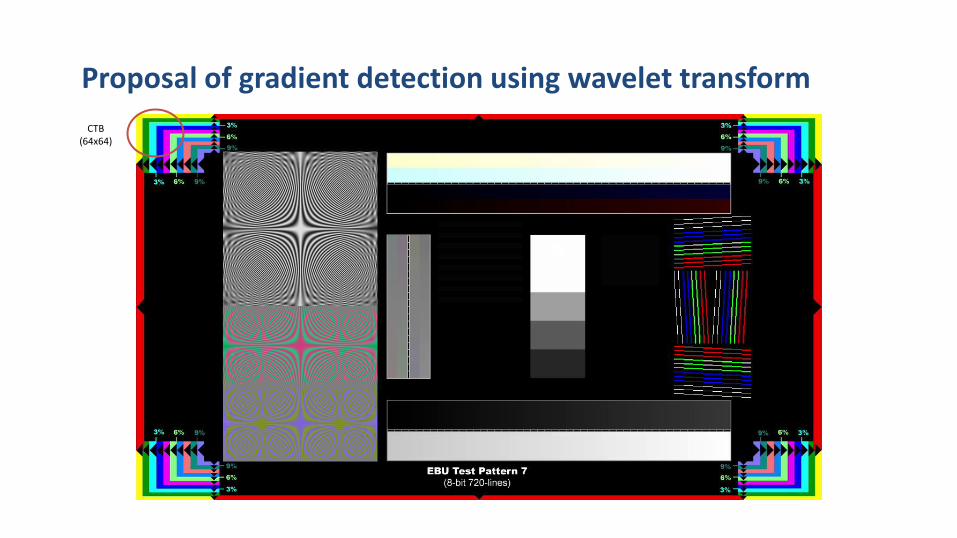
Proposal of gradient detection using wavelet transform

The RMD evaluates the 35 prediction modes, for each of five PU sizes, and in sequential order

Our proposal replaces the RMD stage by using a directional wavelet (directionlet) transform, which allows to detect the dominant gradient of the PU.

Our approach can be computed in parallel, and is specially suitable for multi-core graphic processors.

The algorithm reduces also the number of candidates modes from 8 (RMD) to 3 modes ( four modes for diagonal direction)

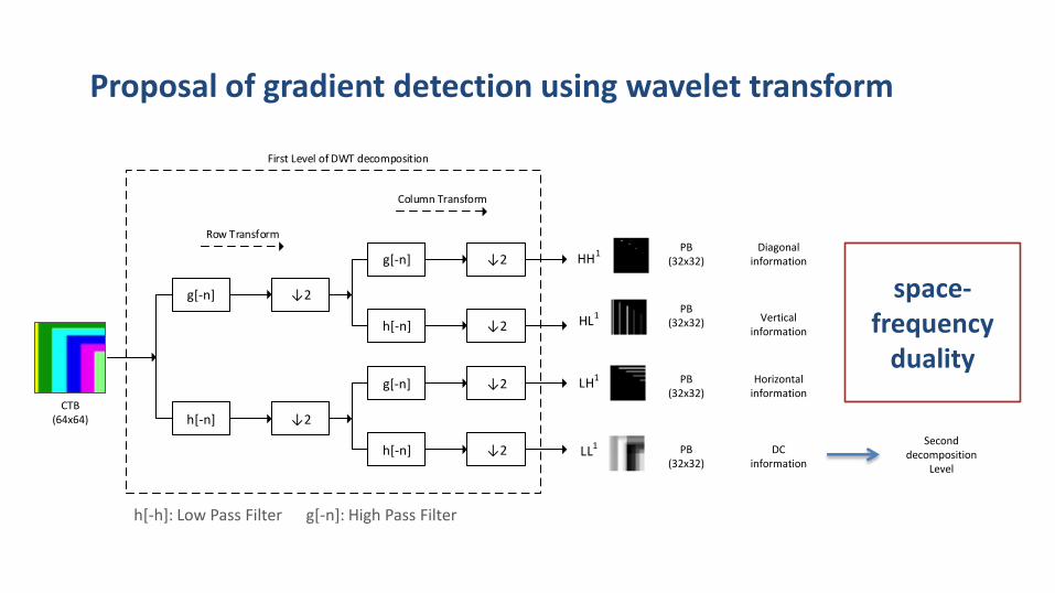
Proposal of gradient detection using wavelet transform

Conventional 2D-Wavelets transform can be implemented as two separated 1D FIR filtering over the rows and columns of the image.

The results are four sub-bands images achieving information of edge with Horizontal (LH1), Vertical (HL1), diagonal (HH1) orientations, and DC (LL1).

The LL sub-band can be newly processed using 2D wavelet transform, achieving four sub-bands of the second decomposition level (LH2,HL2, HH2, LL2).

Traditional Wavelet Transforms (WT) has been shown to be an efficient tool for edge detection and textures classification

Proposal of gradient detection using wavelet transform

CTB (64x64)

Proposal of gradient detection using wavelet transform

CTB (64x64)

g[-n] ↓2

h[-n] ↓2

Row Transform

Column Transform

First Level of DWT decomposition

g[-n] ↓2

h[-n] ↓2

g[-n] ↓2

h[-n] ↓2

HH1

HL1

LH1

LL1

h[-h]: Low Pass Filter g[-n]: High Pass Filter

PB (32x32)

PB (32x32)

PB (32x32)

PB (32x32)

Diagonal information

Vertical information

Horizontal information

DC information

Second decomposition

Level

space-frequency

duality

Proposal of gradient detection using wavelet transform

CTB(64x64)

Four Level Haar DWT

decomposition

Proposal of gradient detection using wavelet transform Rows and column DWT provides poor information for gradients other than rows and columns transform directions (0º, 90º)

In order to estimate the 33 intra prediction directions in HEVC, we need to achieve a gradient information in additional directions.

Four Level Haar DWT

decomposition

CTB (64x64)

Proposal of gradient detection using wavelet transform We compute 10 additional 1D

wavelet transform with rational directions (dy/dx) Example how to get the 10 additional 1D-DWT:

1. 8x8 block is transformed into 10 lines each one of different length: R7=(p1,p2,p3,p4,p5) R10=(p6,p7) … 2. Over this lines apply 1D-DWT get to sublines size N/2 3. Measure the energy of the coefficients to see in which direction we have less high frequencies indicating that this direction is more homogeneous

Proposal of gradient detection using wavelet transform

The 10 directions were selected in a way so that all directions can be calculated for all PU sizes. Making sure that each line has at least two points so its well defined The conventional row and columns wavelets transform, in addition to this new directions, conform a set of 12 ´ri´ gradient directions. But only three slopes match with the HEVC angular modes:

• r3 = H10 • r6 = D18

• r9 = V26

r7= -2 r8= -4 r9= ∞ r10= 4 r11= 2

r0 = 1

r1= 1/2

r2= 1/4

r3= 0

r4= -1/4

r5= -1/2

r6= -1

Proposal of gradient detection using wavelet transform

We define 12 Classes (Ci), defining a set of candidate modes to each Class according to directional transform with slope ‘ri’.

Class

Transform

Direction

Slope

(dy/dx) ϕ Candidate modes

I r0 1/1 225º H2, H3, V33, V34

II r1 1/2 206.6º H4, H5, H6

III r2 1/4 194º H7, H8

IV r3 0 180º H9, H10, H11

V r4 -1/4 166º H12, H13

VI r5 -1/2 153.4º H14, H15, H16

VII r6 -1/1 135º H17, D18, V19

VIII r7 -2/1 116.6º V20, V21, V22

IX r8 -4/1 104º V23, V24

X r9 ∞ 90º V25, V26, V27

XI r10 4/1 76º V28, V29

XII r11 2/1 63.4º V30, V31, V32

Proposal of gradient detection using wavelet transform Each wavelet coefficient Cλ φ

(i,j) in level λ and direction φ, provides frecuencial information related to co-located (2 λ x 2 λ) pixels of CTB

o Coeficients of λ=2 contain gradient information of PB4x4

o Coeficients of λ=3 contain gradient information of PB8x8

o Coeficients of λ=4 contain gradient information of PB16x16

o Coeficients of λ=5 contain gradient information of PB32x32

o Coeficients of λ=6 contain gradient information of PB64x64

For each PUNxN the dominant gradient φ is selected as the maximum Cλ φ

(i,j) at level λ=log2N

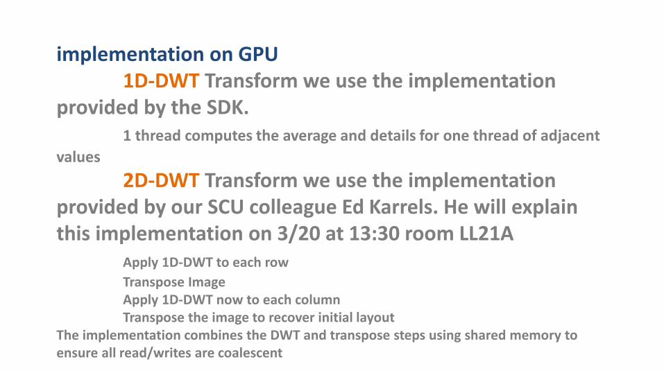
implementation on GPU 1D-DWT Transform we use the implementation provided by the SDK. 1 thread computes the average and details for one thread of adjacent

values

2D-DWT Transform we use the implementation provided by our SCU colleague Ed Karrels. He will explain this implementation on 3/20 at 13:30 room LL21A Apply 1D-DWT to each row

Transpose Image Apply 1D-DWT now to each column Transpose the image to recover initial layout The implementation combines the DWT and transpose steps using shared memory to ensure all read/writes are coalescent

implementation on GPU get 1 frame Repeat 6 times 1 kernel tile image in blocks of size NxN (N starts at 64) Apply the 2D-DWT transform calculate energy of coefficients getting the H, V and D direction 2 kernel reads the block creating the 10 lines and pass this as an input to the 1D-DWT transform calculate energy of the 10 direction select the gradient for the NxN PU as the one with less high Frequency components of the 12

Simulation results

We ha used two 4K sequences (Class A) and five HD sequences (Class B), recommended by the JCT-VC, according to:

JCT-VC, “Common test conditions and software reference configurations,” Join collaborative Team on video Coding 9th meeting, Doc. JCTVC-I1100, 2012.

4K and HD Test sequences Processing a total of 1.502.240

CTBs

Simulation results of HEVC implementation PC with an Intel Core i7-2600 3.40 GHz processor, with 8GB RAM V. Studio 2013, and W7 O.S. Nvidia GTX 690 4096MB, 3072 CUDA cores Computed the average RMD time consumed by CTB, frame and sequence

Class Sequence Frames RMD/CTB

(ms)

RMD/Frame

(sec)

RMD/Sequence

(sec)

Class A Traffic 150 6.053 6.047 907.050

PeopleOnStreet 150 6.096 6.090 913.500

BasketballDrive 500 6.116 3.113 1556.560

BQTerrace 600 6.083 3.096 1857.630

Class B Cactus 500 6.200 3.156 1578.120

Kimono 240 5.961 3.034 728.160

ParkScene 240 5.972 3.046 729.670

Time consuming of RMD in HM implementation

≈ 6ms/CTB

Our Implementation in GPU reach an average speedup of 30%

Conclusions Presented a new approach for accelerating the CU angular decision of the HEVC intra prediction step based on the DWT transform The approach is scalable and suitable for GPU architectures Can be integrated with other algorithms Reduces the time compared with the reference HM standard model

Thank you for your attention

Questions?

Presenter Information

(Name & Organization)