Almost k-Wise Independent Sets

Establish Hitting Sets for

Width-3 1-Branching Programs

Jirı Sıma, Stanislav Zak

Institute of Computer ScienceAcademy of Sciences of the Czech Republic

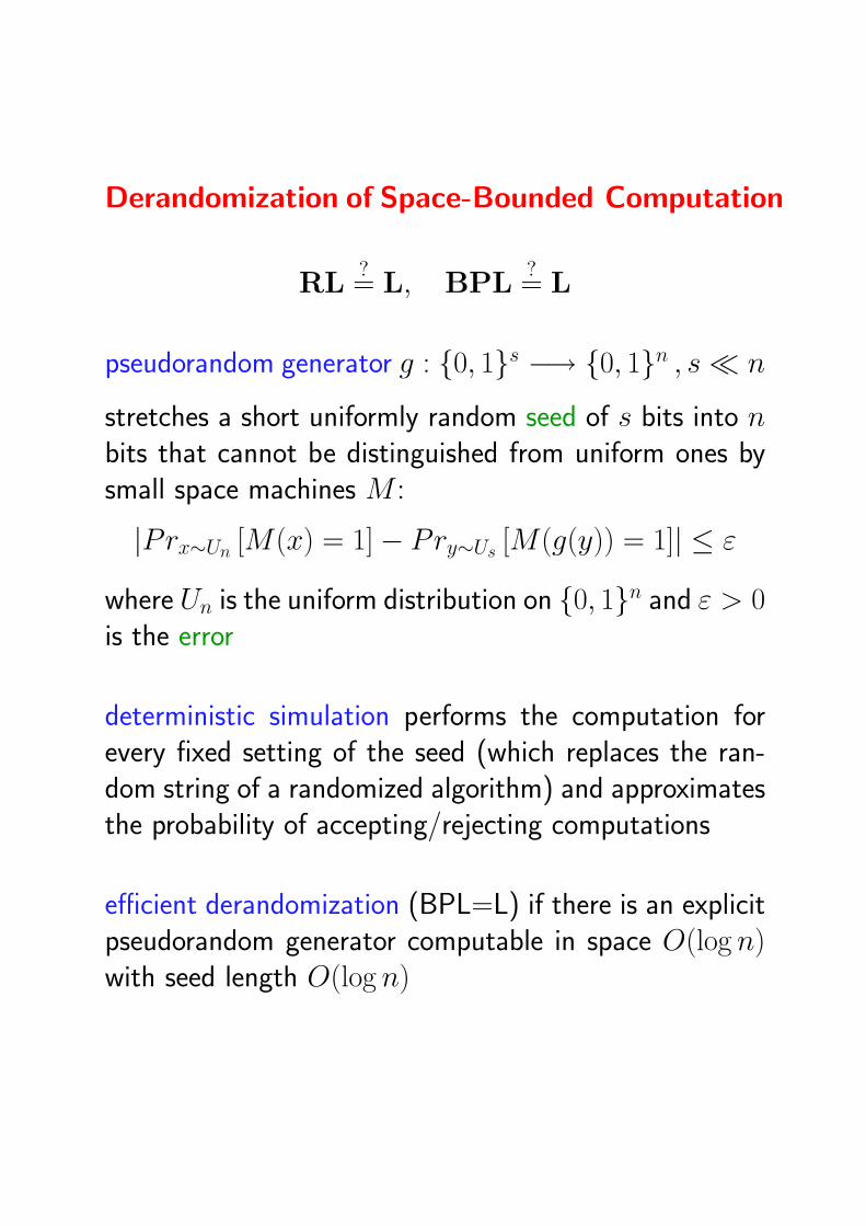
Derandomization of Space-Bounded Computation

RL?= L, BPL

?= L

pseudorandom generator g : 0, 1s −→ 0, 1n , s ¿ n

stretches a short uniformly random seed of s bits into nbits that cannot be distinguished from uniform ones bysmall space machines M :

|Prx∼Un [M(x) = 1]− Pry∼Us [M(g(y)) = 1]| ≤ ε

where Un is the uniform distribution on 0, 1n and ε > 0is the error

deterministic simulation performs the computation forevery fixed setting of the seed (which replaces the ran-dom string of a randomized algorithm) and approximatesthe probability of accepting/rejecting computations

efficient derandomization (BPL=L) if there is an explicitpseudorandom generator computable in space O(log n)with seed length O(log n)

Branching Program P

a leveled directed acyclic multi-graph G = (V, E):

• one source s ∈ V of zero in-degree at level 0

• two sinks of zero out-degree at the last level d (=depth)

• every inner (=non-sink) node has out-degree 2

• the inner nodes are labeled with input Booleanvariables x1, . . . , xn

• the two edges outgoing from any inner node at level` < d lead to nodes at the next level ` + 1 and arelabeled 0 and 1

• the two sinks are labeled 0 and 1

width = the maximum number of nodes in one level

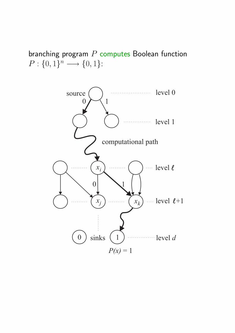
branching program P computes Boolean functionP : 0, 1n −→ 0, 1:

Branching Programs (BPs)

a non-uniform model of space bounded computation:

infinite family of branching programs Pn, one Pn foreach input length n ≥ 1

a computation that uses space s(n) and runs in timet(n) is modeled by Pn of width 2s(n) and depth t(n)(e.g. TM’s configurations are represented by BP’s nodes)

Klivans, van Melkebeek, 1999: if DSPACE(O(n)) re-quires branching programs of size 2Ω(n), then BPL=L.

Restrictions:

Read-Once BPs (1-BPs): every input variable is testedat most once along each computational path

Oblivious BPs: at each level only one variable is queried

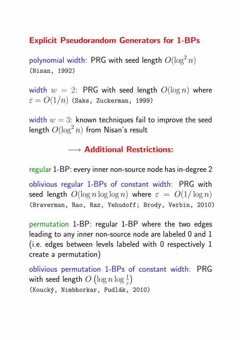
Explicit Pseudorandom Generators for 1-BPs

polynomial width: PRG with seed length O(log2 n)(Nisan, 1992)

width w = 2: PRG with seed length O(log n) whereε = O(1/n) (Saks, Zuckerman, 1999)

width w = 3: known techniques fail to improve the seedlength O(log2 n) from Nisan’s result

−→ Additional Restrictions:

regular 1-BP: every inner non-source node has in-degree 2

oblivious regular 1-BPs of constant width: PRG withseed length O(log n log log n) where ε = O(1/ log n)(Braverman, Rao, Raz, Yehudoff; Brody, Verbin, 2010)

permutation 1-BP: regular 1-BP where the two edgesleading to any inner non-source node are labeled 0 and 1(i.e. edges between levels labeled with 0 respectively 1create a permutation)

oblivious permutation 1-BPs of constant width: PRGwith seed length O

(log n log 1

ε

)(Koucky, Nimbhorkar, Pudlak, 2010)

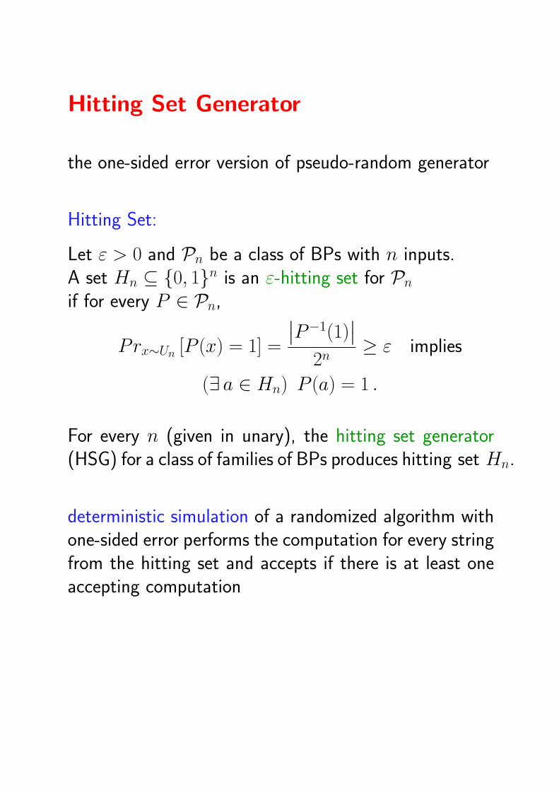
Hitting Set Generator

the one-sided error version of pseudo-random generator

Hitting Set:

Let ε > 0 and Pn be a class of BPs with n inputs.A set Hn ⊆ 0, 1n is an ε-hitting set for Pn

if for every P ∈ Pn,

Prx∼Un [P (x) = 1] =

∣∣P−1(1)∣∣

2n≥ ε implies

(∃ a ∈ Hn) P (a) = 1 .

For every n (given in unary), the hitting set generator(HSG) for a class of families of BPs produces hitting set Hn.

deterministic simulation of a randomized algorithm withone-sided error performs the computation for every stringfrom the hitting set and accepts if there is at least oneaccepting computation

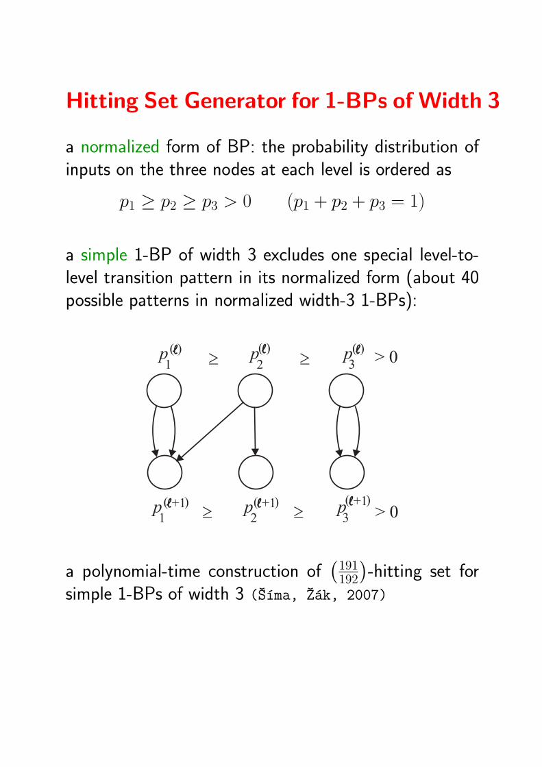
Hitting Set Generator for 1-BPs of Width 3

a normalized form of BP: the probability distribution ofinputs on the three nodes at each level is ordered as

p1 ≥ p2 ≥ p3 > 0 (p1 + p2 + p3 = 1)

a simple 1-BP of width 3 excludes one special level-to-level transition pattern in its normalized form (about 40possible patterns in normalized width-3 1-BPs):

a polynomial-time construction of(

191192

)-hitting set for

simple 1-BPs of width 3 (Sıma, Zak, 2007)

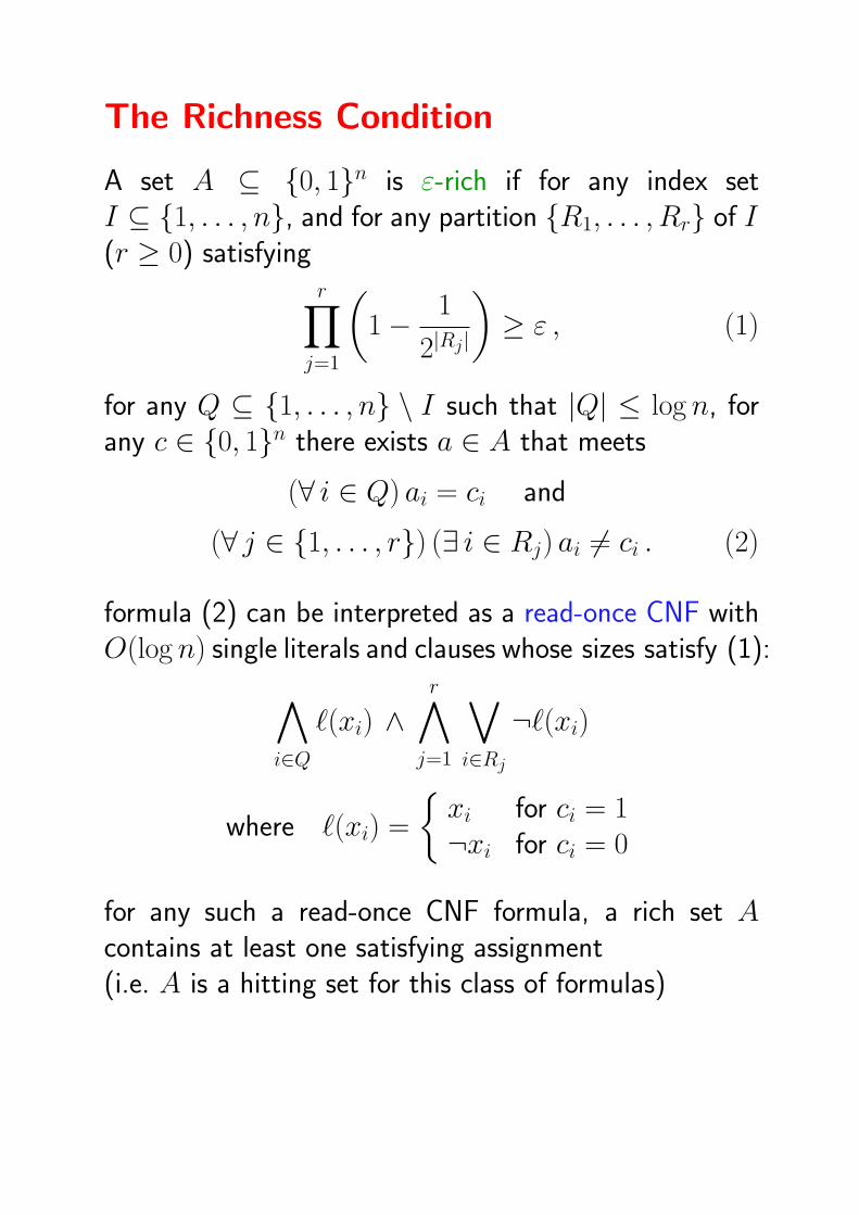
The Richness Condition

A set A ⊆ 0, 1n is ε-rich if for any index setI ⊆ 1, . . . , n, and for any partition R1, . . . , Rr of I(r ≥ 0) satisfying

r∏j=1

(1− 1

2|Rj|

)≥ ε , (1)

for any Q ⊆ 1, . . . , n \ I such that |Q| ≤ log n, forany c ∈ 0, 1n there exists a ∈ A that meets

(∀ i ∈ Q) ai = ci and

(∀ j ∈ 1, . . . , r) (∃ i ∈ Rj) ai 6= ci . (2)

formula (2) can be interpreted as a read-once CNF withO(log n) single literals and clauses whose sizes satisfy (1):

∧

i∈Q

`(xi) ∧r∧

j=1

∨

i∈Rj

¬`(xi)

where `(xi) =

xi for ci = 1¬xi for ci = 0

for any such a read-once CNF formula, a rich set Acontains at least one satisfying assignment(i.e. A is a hitting set for this class of formulas)

Sufficiency of the Richness Condition

the richness condition expresses an essential property ofhitting sets for 1-BPs of width 3 while being independentof a rather technical formalism of branching programs:

Theorem 1 Let ε > 56. If A is ε′11-rich for some ε′ < ε,

then H = Ω3(A) which contains all the vectors withinthe Hamming distance of 3 from any a ∈ A, is anε-hitting set for the class of 1-BPs of width 3.

Idea of proof:

• on the contrary, a normalized 1-BP P of width 3such that

∣∣P−1(1)∣∣ /2n ≥ ε and P (a) = 0 for every

a ∈ H, is assumed

• starting from the last level, the structure of P is in-ductively analyzed block after block (correspondingto partition classes Rj) until a set Q (|Q| ≤ log n)suitable for the richness condition is found

• the richness condition is employed to achieve acontradiction

• the proof includes a rather tedious case analysis, e.g.decreasing the lower bound for ε from the original√

12/13 to 5/6 increases significantly the number ofcases to be analyzed

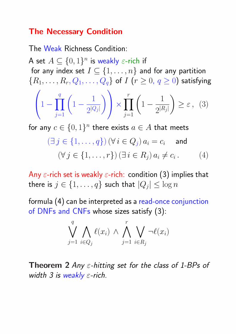
The Necessary Condition

The Weak Richness Condition:

A set A ⊆ 0, 1n is weakly ε-rich iffor any index set I ⊆ 1, . . . , n and for any partitionR1, . . . , Rr, Q1, . . . , Qq of I (r ≥ 0, q ≥ 0) satisfying1−

q∏j=1

(1− 1

2|Qj|

)×

r∏j=1

(1− 1

2|Rj|

)≥ ε , (3)

for any c ∈ 0, 1n there exists a ∈ A that meets

(∃ j ∈ 1, . . . , q) (∀ i ∈ Qj) ai = ci and

(∀ j ∈ 1, . . . , r) (∃ i ∈ Rj) ai 6= ci . (4)

Any ε-rich set is weakly ε-rich: condition (3) implies thatthere is j ∈ 1, . . . , q such that |Qj| ≤ log n

formula (4) can be interpreted as a read-once conjunctionof DNFs and CNFs whose sizes satisfy (3):

q∨j=1

∧

i∈Qj

`(xi) ∧r∧

j=1

∨

i∈Rj

¬`(xi)

Theorem 2 Any ε-hitting set for the class of 1-BPs ofwidth 3 is weakly ε-rich.

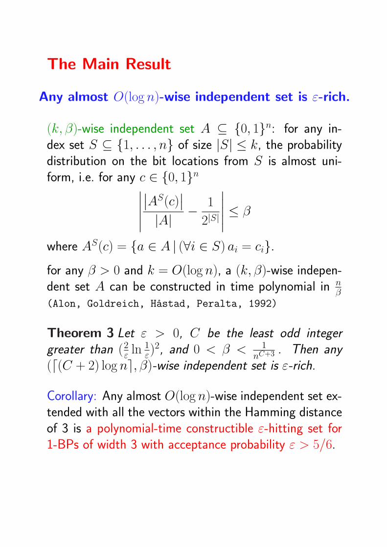
The Main Result

Any almost O(log n)-wise independent set is ε-rich.

(k, β)-wise independent set A ⊆ 0, 1n: for any in-dex set S ⊆ 1, . . . , n of size |S| ≤ k, the probabilitydistribution on the bit locations from S is almost uni-form, i.e. for any c ∈ 0, 1n

∣∣∣∣∣

∣∣AS(c)∣∣

|A| − 1

2|S|

∣∣∣∣∣ ≤ β

where AS(c) = a ∈ A | (∀i ∈ S) ai = ci.for any β > 0 and k = O(log n), a (k, β)-wise indepen-dent set A can be constructed in time polynomial in n

β(Alon, Goldreich, Hastad, Peralta, 1992)

Theorem 3 Let ε > 0, C be the least odd integergreater than (2

ε ln 1ε)

2, and 0 < β < 1nC+3 . Then any

(d(C + 2) log ne, β)-wise independent set is ε-rich.

Corollary: Any almost O(log n)-wise independent set ex-tended with all the vectors within the Hamming distanceof 3 is a polynomial-time constructible ε-hitting set for1-BPs of width 3 with acceptance probability ε > 5/6.

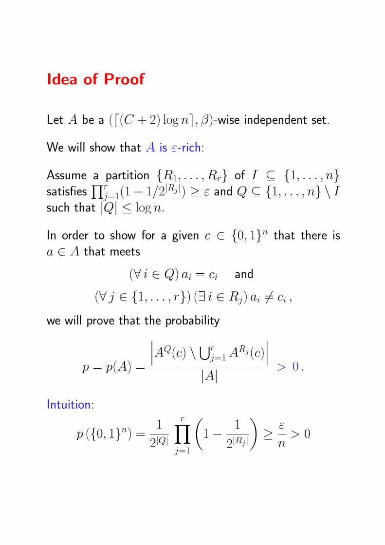
Idea of Proof

Let A be a (d(C + 2) log ne, β)-wise independent set.

We will show that A is ε-rich:

Assume a partition R1, . . . , Rr of I ⊆ 1, . . . , nsatisfies

∏rj=1(1− 1/2|Rj|) ≥ ε and Q ⊆ 1, . . . , n \ I

such that |Q| ≤ log n.

In order to show for a given c ∈ 0, 1n that there isa ∈ A that meets

(∀ i ∈ Q) ai = ci and

(∀ j ∈ 1, . . . , r) (∃ i ∈ Rj) ai 6= ci ,

we will prove that the probability

p = p(A) =

∣∣∣AQ(c) \⋃rj=1 ARj(c)

∣∣∣|A| > 0 .

Intuition:

p (0, 1n) =1

2|Q|

r∏j=1

(1− 1

2|Rj|

)≥ ε

n> 0

The Main Steps of the Proof

Modifications of Partition Classes:

• superlogarithmic cardinalities:

R′j ⊆ Rj so that |R′

j| ≤ log n

• small constant cardinalities:

R≤σ =⋃|R′j|≤σ R′

j where σ is a suitable constant

−→ Q′ = Q ∪R≤σ, c′i = 1− ci for i ∈ R≤σ

Lemma: p ≥

∣∣∣AQ′(c′) \⋃r′j=1 AR′j(c′)

∣∣∣|A|

Bonferroni inequality

p ≥C ′∑

k=0

(−1)k∑

1≤j1<j2<···<jk≤r′

∣∣∣A⋃k

i=1 R′ji∪Q′(c′)

∣∣∣|A|

Almost O(log n)-wise independence

p ≥ 1

2|Q′|

C ′∑

k=0

(−1)k∑

1≤j1<j2<···<jk≤r′

k∏i=1

1

2

∣∣∣R′ji∣∣∣− ε′

8

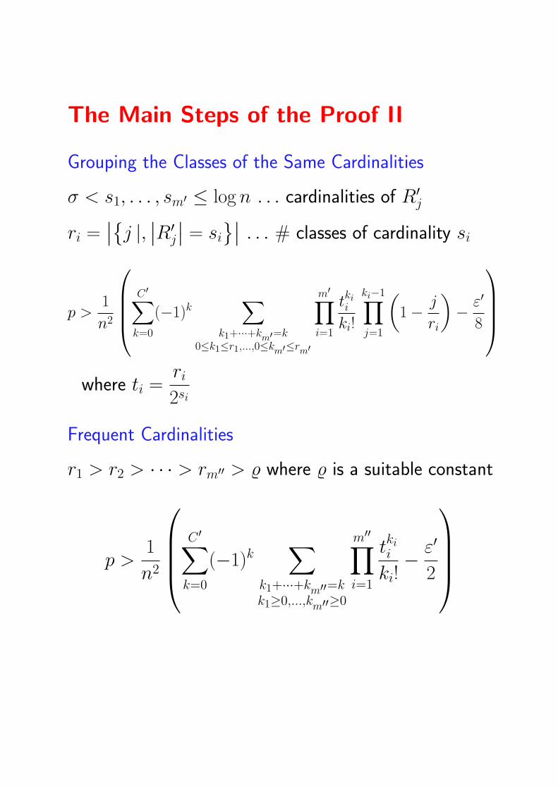
The Main Steps of the Proof II

Grouping the Classes of the Same Cardinalities

σ < s1, . . . , sm′ ≤ log n . . . cardinalities of R′j

ri =∣∣j |, ∣∣R′

j

∣∣ = si

∣∣ . . . # classes of cardinality si

p >1

n2

C ′∑

k=0

(−1)k∑

k1+···+km′=k0≤k1≤r1,...,0≤km′≤rm′

m′∏i=1

tkii

ki!

ki−1∏j=1

(1− j

ri

)− ε′

8

where ti =ri

2si

Frequent Cardinalities

r1 > r2 > · · · > rm′′ > % where % is a suitable constant

p >1

n2

C ′∑

k=0

(−1)k∑

k1+···+km′′=kk1≥0,...,km′′≥0

m′′∏i=1

tkii

ki!− ε′

2

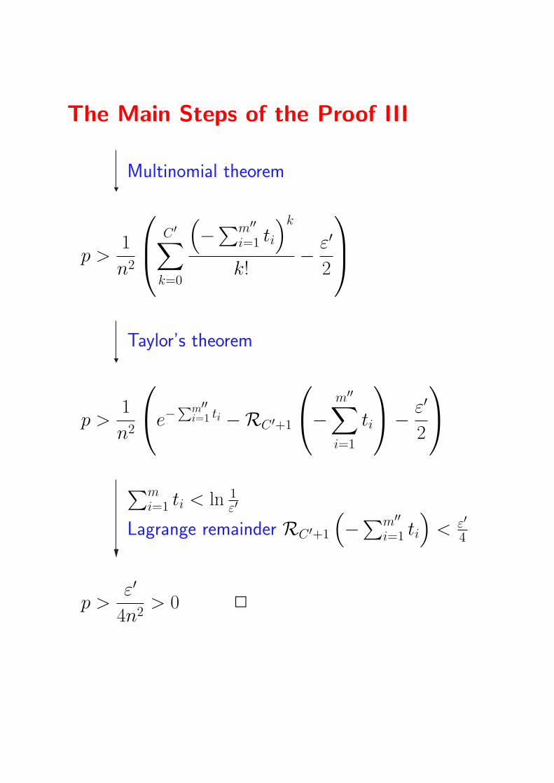
The Main Steps of the Proof III

Multinomial theorem

p >1

n2

C ′∑

k=0

(−∑m′′

i=1 ti

)k

k!− ε′

2

Taylor’s theorem

p >1

n2

e−

∑m′′i=1 ti −RC ′+1

−

m′′∑i=1

ti

− ε′

2

∑mi=1 ti < ln 1

ε′

Lagrange remainder RC ′+1

(−∑m′′

i=1 ti

)< ε′

4

p >ε′

4n2> 0 2

Conclusion & Open Problems

• the explicit polynomial-time construction of a hittingset for 1-BPs of width 3

• an important step in the effort to construct HSGs for1-BPs of bounded width

×such constructions were known only for width 2 andfor oblivious regular/permutation 1-BPs of boundedwidth

• Can the result be achieved for any acceptanceprobability ε > 0 (× our result holds for ε > 5/6) ?

• Can the technique be extended to width 4 or to boundedwidth ?