CSIS 625 1

CSIS 625 Week 3

Transmission Media, Multiplexing

Copyright 2001 - Dan Oelke

For use by students of CSIS 625 for purposes of this class only.

CSIS 625 2

Overview

• Transmission Media– Wired - Twisted Pair, Coax, Fiber– Wireless– Impairments

• Multiplexing– Space, Frequency, Wave– Synchronous & Statistical Time multiplexing– Traffic Engineering

CSIS 625 3

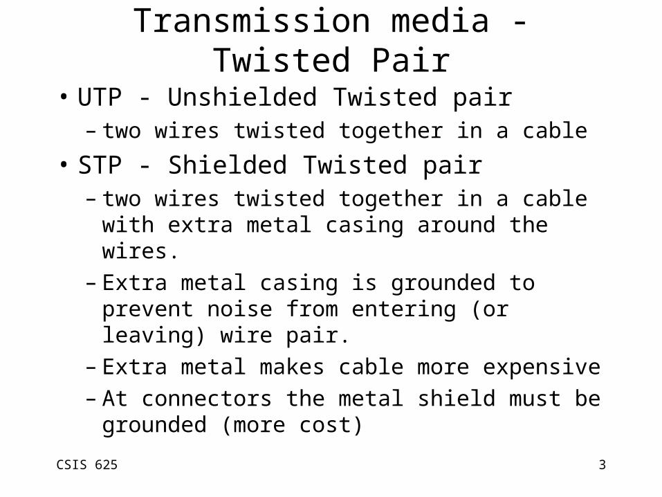
Transmission media - Twisted Pair

• UTP - Unshielded Twisted pair– two wires twisted together in a cable

• STP - Shielded Twisted pair– two wires twisted together in a cable with extra

metal casing around the wires. – Extra metal casing is grounded to prevent noise

from entering (or leaving) wire pair.– Extra metal makes cable more expensive– At connectors the metal shield must be

grounded (more cost)

CSIS 625 4

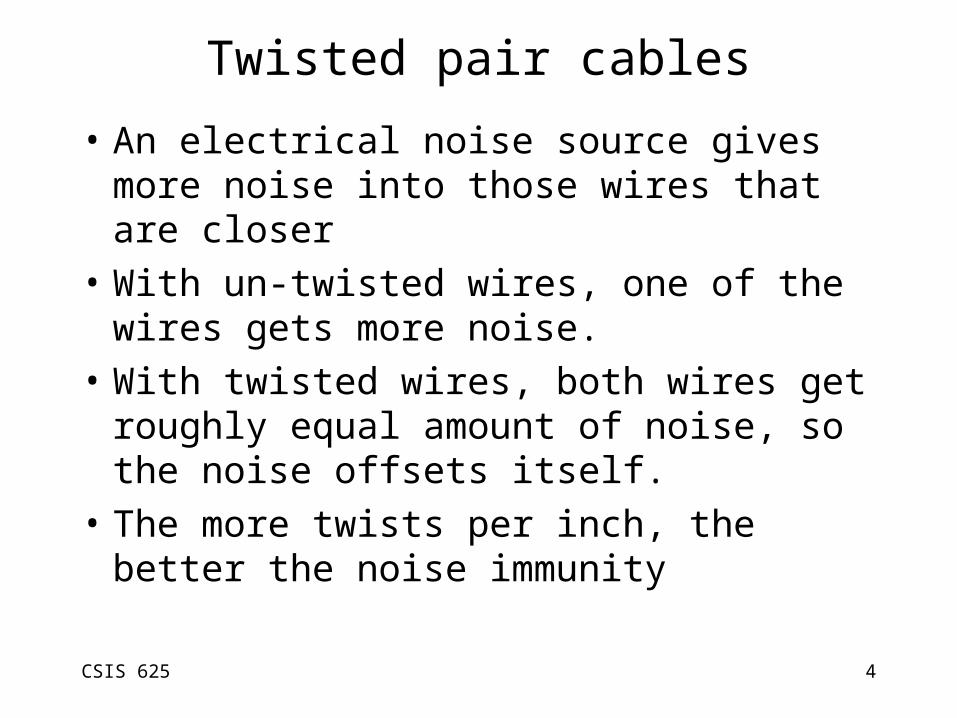
Twisted pair cables

• An electrical noise source gives more noise into those wires that are closer

• With un-twisted wires, one of the wires gets more noise.

• With twisted wires, both wires get roughly equal amount of noise, so the noise offsets itself.

• The more twists per inch, the better the noise immunity

CSIS 625 5

Twisted pair cables

• The more twists per inch, the more copper (and cost) in a cable.

• When multiple pairs are in a single cable, each of the pairs should be twisted at a slightly different number of twists per inch.– To prevent one pair creating noise in another

pair.

CSIS 625 6

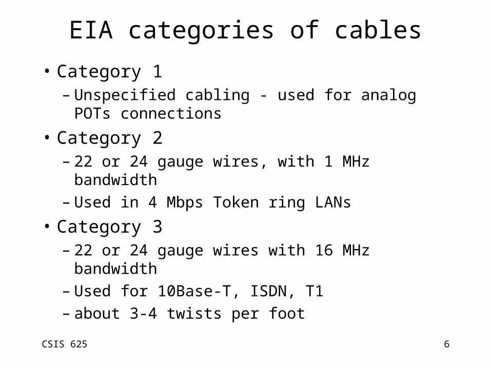
EIA categories of cables

• Category 1– Unspecified cabling - used for analog POTs

connections

• Category 2– 22 or 24 gauge wires, with 1 MHz bandwidth– Used in 4 Mbps Token ring LANs

• Category 3– 22 or 24 gauge wires with 16 MHz bandwidth– Used for 10Base-T, ISDN, T1– about 3-4 twists per foot

CSIS 625 7

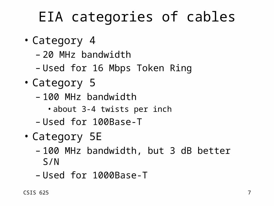
EIA categories of cables

• Category 4– 20 MHz bandwidth– Used for 16 Mbps Token Ring

• Category 5– 100 MHz bandwidth

• about 3-4 twists per inch

– Used for 100Base-T

• Category 5E– 100 MHz bandwidth, but 3 dB better S/N– Used for 1000Base-T

CSIS 625 8

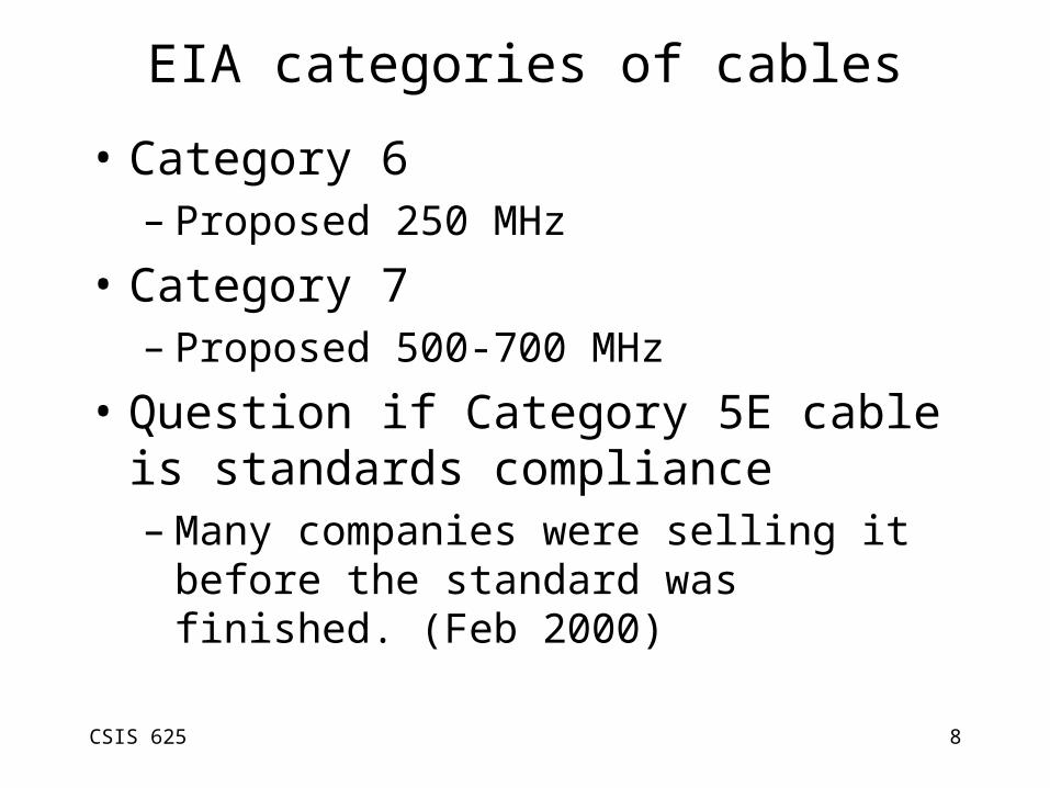
EIA categories of cables

• Category 6– Proposed 250 MHz

• Category 7– Proposed 500-700 MHz

• Question if Category 5E cable is standards compliance– Many companies were selling it before the

standard was finished. (Feb 2000)

CSIS 625 9

Coax Cable

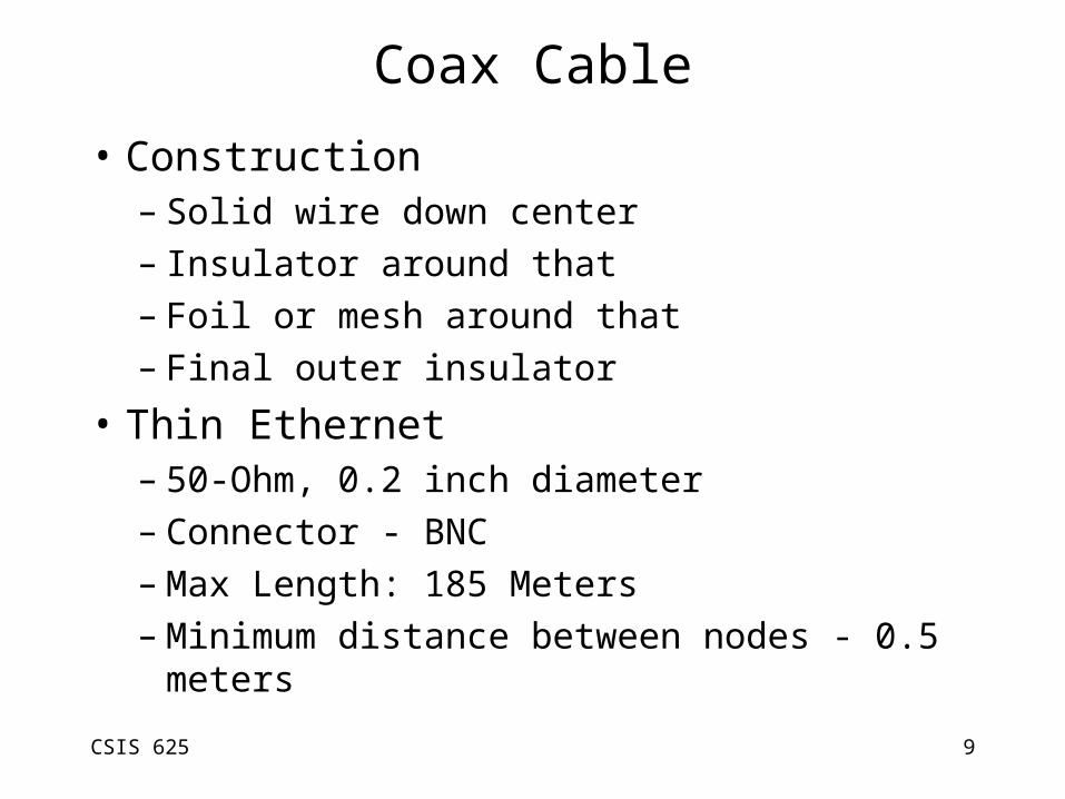
• Construction– Solid wire down center– Insulator around that– Foil or mesh around that– Final outer insulator

• Thin Ethernet– 50-Ohm, 0.2 inch diameter– Connector - BNC– Max Length: 185 Meters– Minimum distance between nodes - 0.5 meters

CSIS 625 10

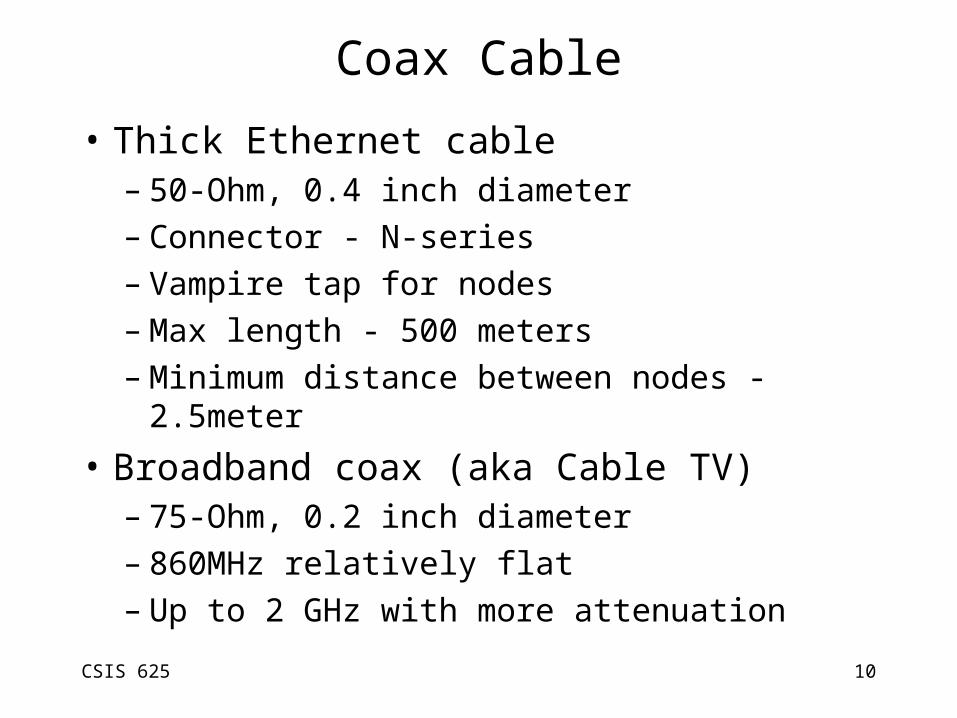
Coax Cable

• Thick Ethernet cable– 50-Ohm, 0.4 inch diameter – Connector - N-series– Vampire tap for nodes– Max length - 500 meters– Minimum distance between nodes - 2.5meter

• Broadband coax (aka Cable TV)– 75-Ohm, 0.2 inch diameter– 860MHz relatively flat– Up to 2 GHz with more attenuation

CSIS 625 11

Eye Diagrams

– A diagram that shows how well a digital signal is transported on a medium.

– Shows amplitude and timing noise– Wide open eye is better than mostly closed one.– Standards often have exclusion zones in the

center and above and below

CSIS 625 12

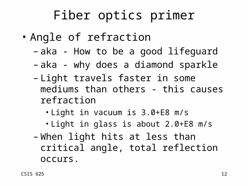
Fiber optics primer

• Angle of refraction– aka - How to be a good lifeguard– aka - why does a diamond sparkle– Light travels faster in some mediums than

others - this causes refraction• Light in vacuum is 3.0+E8 m/s

• Light in glass is about 2.0+E8 m/s

– When light hits at less than critical angle, total reflection occurs.

CSIS 625 13

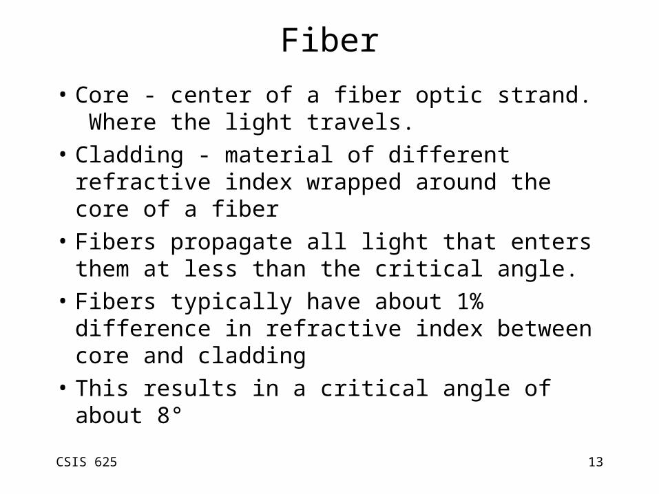
Fiber

• Core - center of a fiber optic strand. Where the light travels.

• Cladding - material of different refractive index wrapped around the core of a fiber

• Fibers propagate all light that enters them at less than the critical angle.

• Fibers typically have about 1% difference in refractive index between core and cladding

• This results in a critical angle of about 8°

CSIS 625 14

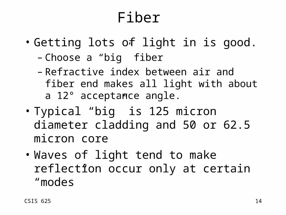
Fiber

• Getting lots of light in is good.– Choose a “big” fiber– Refractive index between air and fiber end

makes all light with about a 12° acceptance angle.

• Typical “big” is 125 micron diameter cladding and 50 or 62.5 micron core

• Waves of light tend to make reflection occur only at certain “modes”

CSIS 625 15

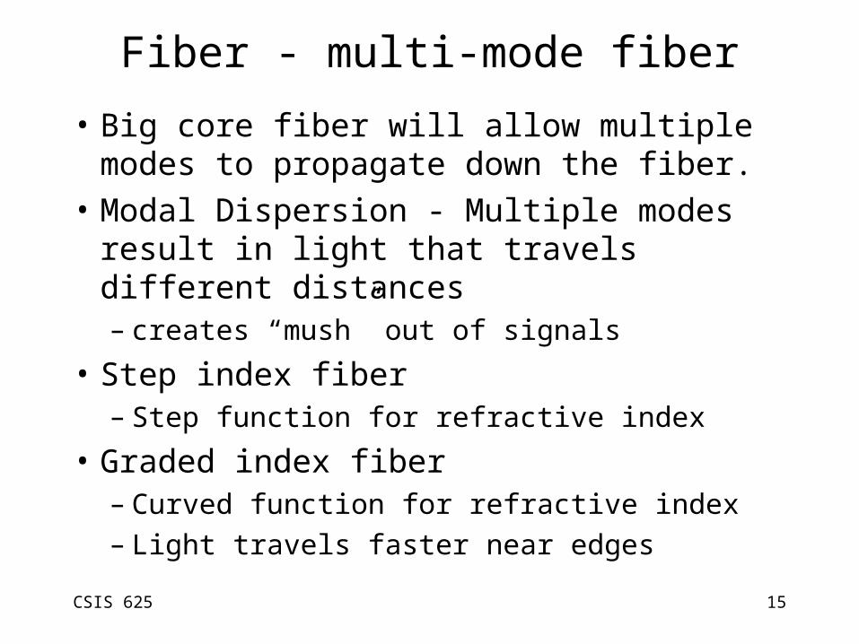
Fiber - multi-mode fiber

• Big core fiber will allow multiple modes to propagate down the fiber.

• Modal Dispersion - Multiple modes result in light that travels different distances– creates “mush” out of signals

• Step index fiber– Step function for refractive index

• Graded index fiber– Curved function for refractive index

– Light travels faster near edges

CSIS 625 16

Multi-mode fiber

• Graded index fiber allows for much farther distances at higher bit rates to be achieved

CSIS 625 17

Fiber - single-mode fiber

• To avoid Modal dispersion - use a smaller fiber where only one mode can travel down the fiber

• Harder to get light in - BUT results in much longer distances being obtainable.

• Single mode fiber is typically 125 micron diameter cladding and 8 micron core.

CSIS 625 18

Fiber light sources - Raleigh Scattering

• aka Why are sunsets red and the sky blue.

• Raleigh Scattering– Blue light is about 400nm wavelength– Red light is about 700nm wavelength– Blue is about 9.4 times more likely to be

scattered than red– From this, we want longer wavelengths to

avoid scattering and keep light headed towards destination

CSIS 625 19

Fiber light sources

• Light absorption of glass – Around 1600 nm wavelength, silica glass light

starts to absorb light

• Water is a common impurity in glass– OH tends to absorb light at various parts

• Graph of loss vs. wavelength– From graph we see that around 1550nm and

around 1310nm are best spots for transmitting– 850nm is also used because of ease of creating

light source

CSIS 625 20

Fiber Dispersion types

• Dispersion - All light does not travel at the same speed down a fiber. This results in sloped edges of optical pulses

• Modal Dispersion - – Different modes of light travel different

distances in multi-mode fiber

• Material Dispersion– Differences in the refractive index in the core

• Careful quality control fixes this

CSIS 625 21

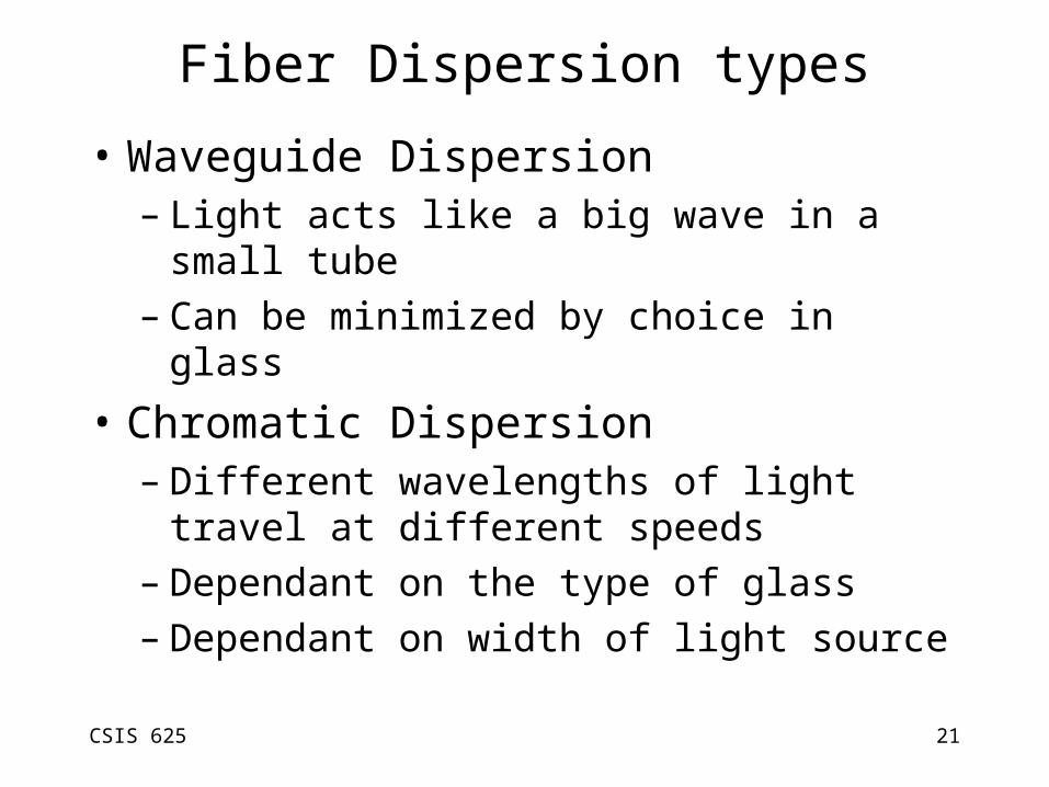
Fiber Dispersion types

• Waveguide Dispersion– Light acts like a big wave in a small tube– Can be minimized by choice in glass

• Chromatic Dispersion– Different wavelengths of light travel at

different speeds– Dependant on the type of glass– Dependant on width of light source

CSIS 625 22

Fiber Dispersion types

• Polarization mode Dispersion– Different refractive indexes in a material based

on the polarization of light. • Different refractive indexes means different speeds

of light.

– Smallest effect • Increases with square root of transmission distance

CSIS 625 23

Fiber’s advantages

• Advantages– Minimal interference– Best bandwidth and distance

• Disadvantages– Slightly more costly

• But may be offset by speed up

– Harder to do a splice

• Security - slight advantage– Contrary to the myth - You can tap a fiber– Not very cheap or easy to do it though.

CSIS 625 24

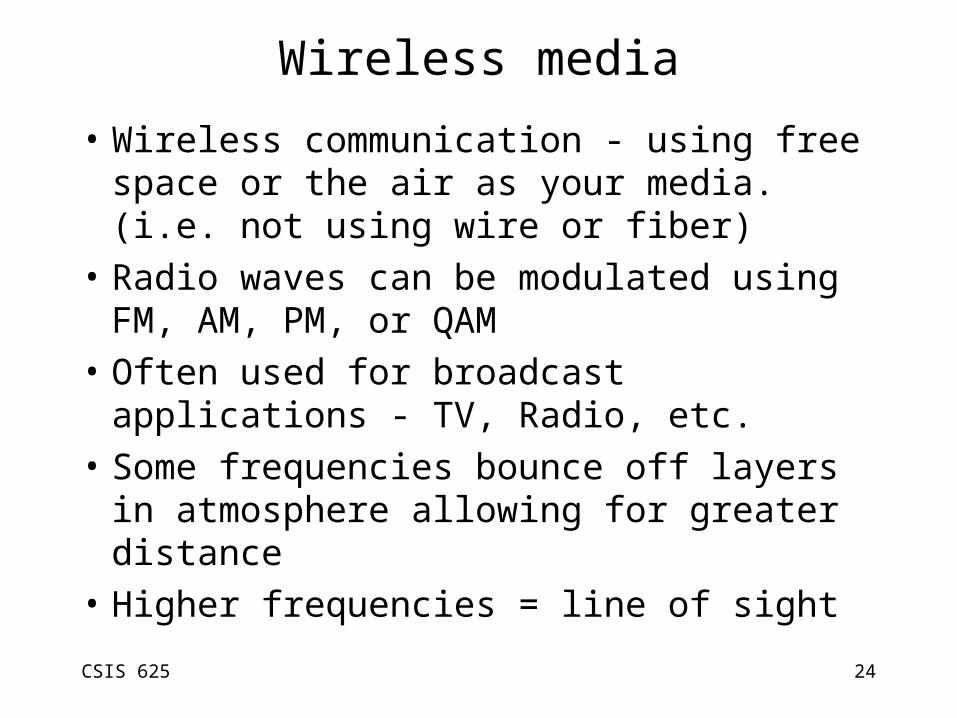
Wireless media

• Wireless communication - using free space or the air as your media. (i.e. not using wire or fiber)

• Radio waves can be modulated using FM, AM, PM, or QAM

• Often used for broadcast applications - TV, Radio, etc.

• Some frequencies bounce off layers in atmosphere allowing for greater distance

• Higher frequencies = line of sight

CSIS 625 25

Frequency Bands

– 0-300 Hz ELF - Extremely low Freq

– 300-3000 Hz ILF - Infra Low Freq

– 3-30 kHz VLF - Very Low Frequency

– 30-300 kHz LF - Low Frequency

– 300-3000 kHz MF - Medium Frequency

– 3-30 MHz HF - High Frequency

– 30-300 MHz VHF - Very High Frequency

– 300-3000 MHz UHF - Ultra High Frequency

– 3-30 GHz SHF - Super High Frequency

– 30-300 GHz EHF - Extremely High Frequency

– 300-3000 GHz THF - Tremendously High Frequency

CSIS 625 26

Wireless Applications

• TV and Radio

• Cellular Telephone

• Satellite Television

• Satellite Telephony and Data

• Wireless LANs

• Much more on this in a future lecture

CSIS 625 27

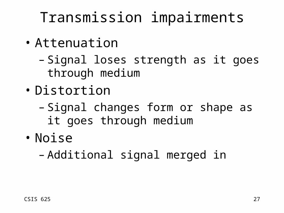
Transmission impairments

• Attenuation– Signal loses strength as it goes through medium

• Distortion– Signal changes form or shape as it goes through

medium

• Noise – Additional signal merged in

CSIS 625 28

Signal Strength

• Decibel (dB) is a measure of the relative strengths of two signals.

• dB = 10 * log10 (P2/P1)

• P1 = Power of signal at point 1

• P2 = Power of signal at point 2

• dB are used because it allows end-to-end signal strength to be determined by adding up attenuations and amplifications

• Signal-Noise Ratio - a dB measurement of signal strength to noise strength

CSIS 625 29

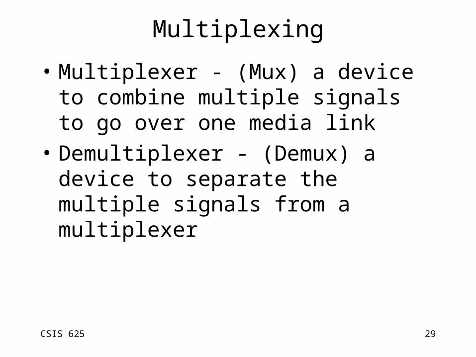
Multiplexing

• Multiplexer - (Mux) a device to combine multiple signals to go over one media link

• Demultiplexer - (Demux) a device to separate the multiple signals from a multiplexer

CSIS 625 30

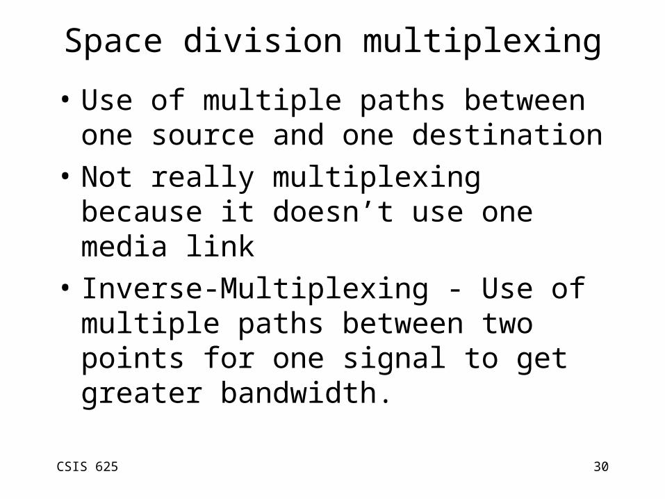
Space division multiplexing

• Use of multiple paths between one source and one destination

• Not really multiplexing because it doesn’t use one media link

• Inverse-Multiplexing - Use of multiple paths between two points for one signal to get greater bandwidth.

CSIS 625 31

Frequency Division multiplexing - FDM

• Use of different carrier frequencies

• Must make sure that the carriers do not overlap

• Guard Band - unused bandwidth between signals that provides protection against overlap

• TV and Radio are most common examples

CSIS 625 32

Telephony FDM

• Telephony before the digital time, used FDM heavily

• AT&T and CCITT came up with slightly different standards

• Lower groups multiplex to higher groups

# VoiceChannels Bandwidth Spectrum AT&T CCITT

12 48kHz 60-108kHz Group Group60 240kHz 312-552kHz Supergroup Supergroup

300 1.232MHz 812-2044kHz Mastergroup600 2.52MHz 564-3084kHz Mastergroup900 3.872MHz 8.516-12.388MHz Supermastergroup

3600 16.984MHz 0.564-17.548MHz Jumbogroup10800 57.442MHz 3.124-60.566MHz Jumbogroup

Multiplex

CSIS 625 33

Wave Division multiplexing (WDM)

• Use of multiple wavelengths of light over a fiber optic system (optical form of FDM)

• CDWM - Coarse WDM– Typically use of 850, 1310nm and 1550nm

wavelengths – Sometimes use of 4 or 8 wavelengths around

1550nm

• DWDM - Dense WDM– Use of many (16-100+) wavelengths around the

1550nm wavelength.

CSIS 625 34

Synchronous Time Division Multiplexing (TDM)

• Multiple signals are carried by interleaving portions of each signal in time.

• Each input signal has exactly the same time slot that occurs repeatedly

• A group of time slots are grouped into a frame

• May occur at bit level, byte level, or blocks of data

• May be done in analog systems as well as digital, but typically seen in digital systems

CSIS 625 35

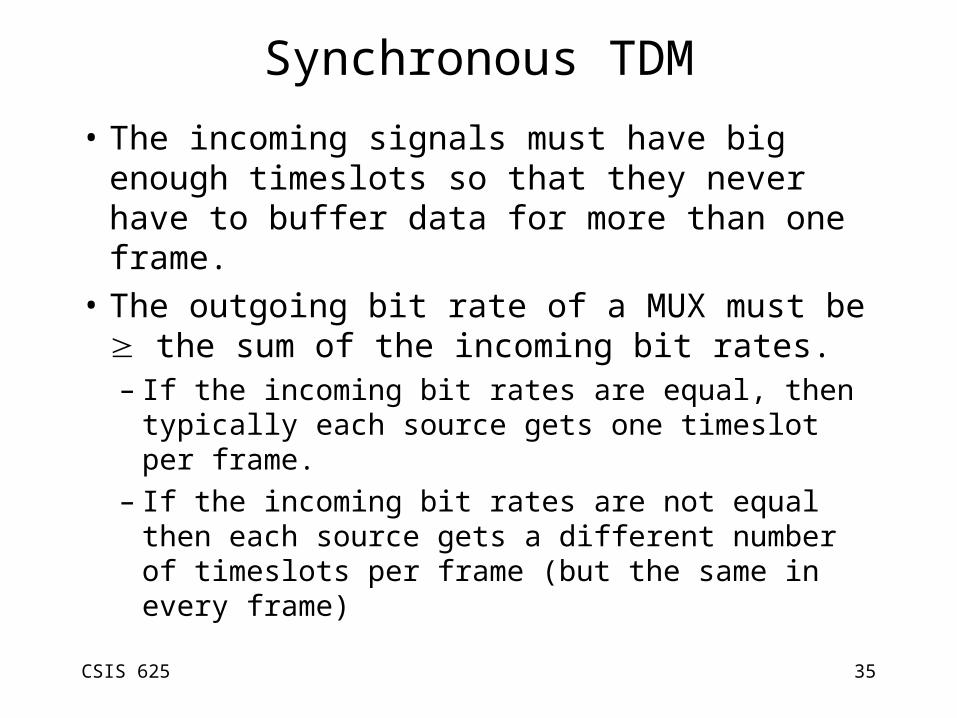
Synchronous TDM

• The incoming signals must have big enough timeslots so that they never have to buffer data for more than one frame.

• The outgoing bit rate of a MUX must be the sum of the incoming bit rates.– If the incoming bit rates are equal, then typically

each source gets one timeslot per frame.– If the incoming bit rates are not equal then each

source gets a different number of timeslots per frame (but the same in every frame)

CSIS 625 36

Synchronous TDM

• So that the DEMUX knows when the timeslots are and who gets which data, there is some framing overhead.– Typically some extra bytes of data at the start

of each frame.

• If the data rate of the incoming signals does not divide evenly into a timeslot, then extra bits may be inserted by the MUX and discarded by the DEMUX.– This is sometimes called bit-stuffing

CSIS 625 37

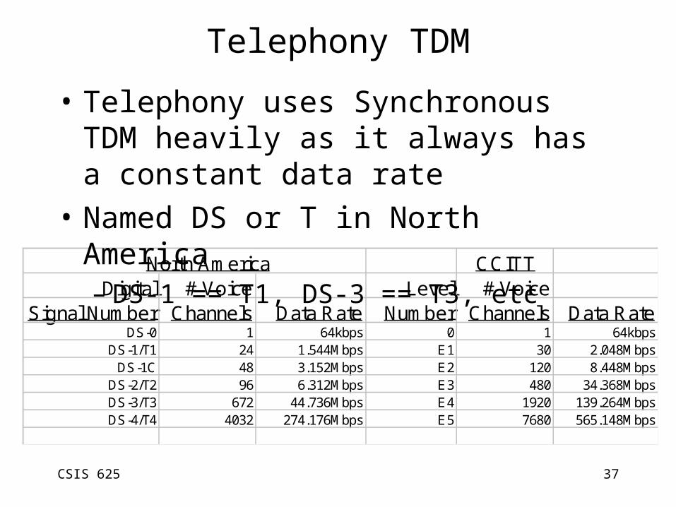
Telephony TDM

North America CCITTDigital # Voice Level # Voice

Signal Number Channels Data Rate Number Channels Data RateDS-0 1 64kbps 0 1 64kbps

DS-1/T1 24 1.544Mbps E1 30 2.048MbpsDS-1C 48 3.152Mbps E2 120 8.448Mbps

DS-2/T2 96 6.312Mbps E3 480 34.368MbpsDS-3/T3 672 44.736Mbps E4 1920 139.264MbpsDS-4/T4 4032 274.176Mbps E5 7680 565.148Mbps

• Telephony uses Synchronous TDM heavily as it always has a constant data rate

• Named DS or T in North America– DS-1 == T1, DS-3 == T3, etc

CSIS 625 38

DS1 circuit

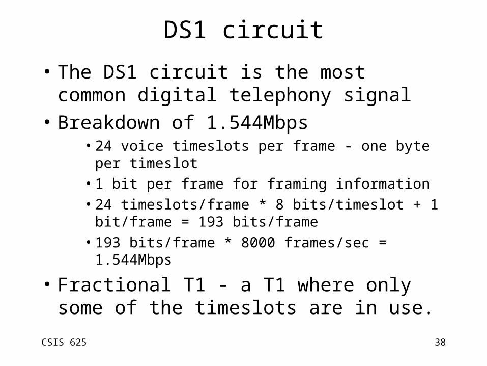
• The DS1 circuit is the most common digital telephony signal

• Breakdown of 1.544Mbps• 24 voice timeslots per frame - one byte per timeslot

• 1 bit per frame for framing information

• 24 timeslots/frame * 8 bits/timeslot + 1 bit/frame = 193 bits/frame

• 193 bits/frame * 8000 frames/sec = 1.544Mbps

• Fractional T1 - a T1 where only some of the timeslots are in use.

CSIS 625 39

T1 - a little more information

• Original D1 channel banks– Used alternating 1/0 pattern in framing bit– Could get confused by 1000Hz tone– Used least significant bit of every data byte for

signaling.

• D2-D4 channel banks– Used 12 bit pattern in framing bit– Used least significant bit data byte for signaling

only in the 6th and 12th frame– This is AB signaling

CSIS 625 40

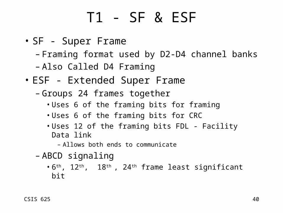
T1 - SF & ESF

• SF - Super Frame – Framing format used by D2-D4 channel banks– Also Called D4 Framing

• ESF - Extended Super Frame– Groups 24 frames together

• Uses 6 of the framing bits for framing

• Uses 6 of the framing bits for CRC

• Uses 12 of the framing bits FDL - Facility Data link– Allows both ends to communicate

– ABCD signaling • 6th, 12th, 18th , 24th frame least significant bit

CSIS 625 41

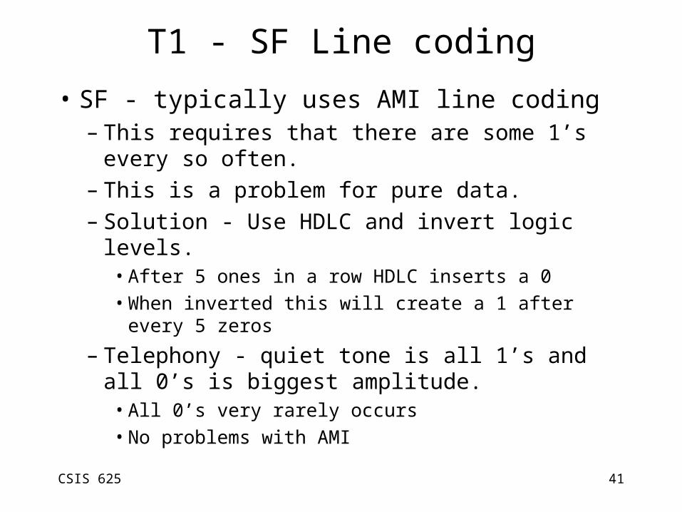
T1 - SF Line coding

• SF - typically uses AMI line coding– This requires that there are some 1’s every so

often.– This is a problem for pure data.– Solution - Use HDLC and invert logic levels.

• After 5 ones in a row HDLC inserts a 0• When inverted this will create a 1 after every 5 zeros

– Telephony - quiet tone is all 1’s and all 0’s is biggest amplitude.

• All 0’s very rarely occurs• No problems with AMI

CSIS 625 42

T1 - ESF Line coding

• ESF - typically uses B8ZS line coding– No Data dependencies – B8ZS makes sure that any data pattern can pass

without problem.

• If you order a T1 from the phone company– Specify ESF– Specify B8ZS– Especially true for data, but true even for

modem traffic or voice traffic• You get better protection and CRC error counts

CSIS 625 43

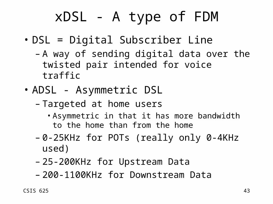
xDSL - A type of FDM

• DSL = Digital Subscriber Line– A way of sending digital data over the twisted

pair intended for voice traffic

• ADSL - Asymmetric DSL– Targeted at home users

• Asymmetric in that it has more bandwidth to the home than from the home

– 0-25KHz for POTs (really only 0-4KHz used)– 25-200KHz for Upstream Data– 200-1100KHz for Downstream Data

CSIS 625 44

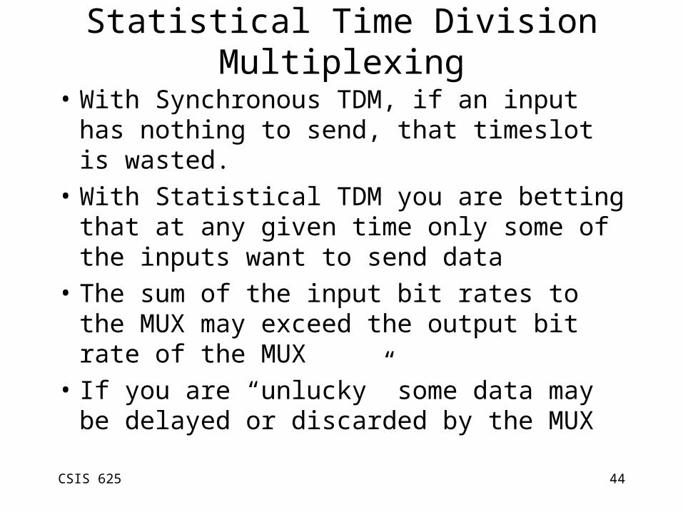
Statistical Time Division Multiplexing

• With Synchronous TDM, if an input has nothing to send, that timeslot is wasted.

• With Statistical TDM you are betting that at any given time only some of the inputs want to send data

• The sum of the input bit rates to the MUX may exceed the output bit rate of the MUX

• If you are “unlucky” some data may be delayed or discarded by the MUX

CSIS 625 45

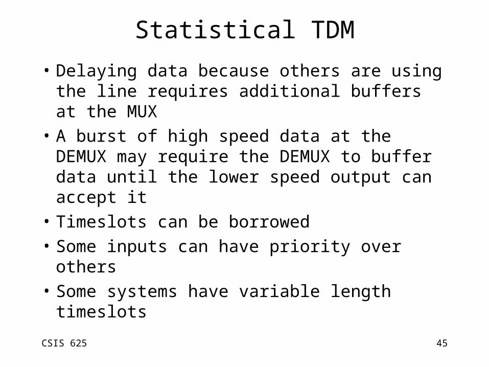
Statistical TDM

• Delaying data because others are using the line requires additional buffers at the MUX

• A burst of high speed data at the DEMUX may require the DEMUX to buffer data until the lower speed output can accept it

• Timeslots can be borrowed

• Some inputs can have priority over others

• Some systems have variable length timeslots

CSIS 625 46

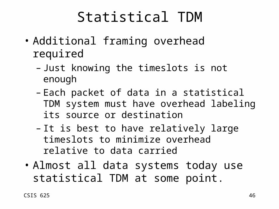
Statistical TDM

• Additional framing overhead required– Just knowing the timeslots is not enough– Each packet of data in a statistical TDM system

must have overhead labeling its source or destination

– It is best to have relatively large timeslots to minimize overhead relative to data carried

• Almost all data systems today use statistical TDM at some point.

CSIS 625 47

Traffic Engineering

• In telephony networks, not all phones are in use at the same time, so trunks between central offices are over-subscribed– This is a form of statistical TDM

• Agner Krarup Erlang (1878-1929)– developed equations on how the blocking

probability relates to the amount of traffic and number of lines.

CSIS 625 48

Traffic Engineering Definitions

• Trunk - a communication line between two switching systems

• Poisson Distribution - A mathematical formula that defines the probability of x events occurring in a certain time

• Busy Hour - The one hour during the day or year that has the most traffic

• CCS - Centum Call Seconds - amount of traffic offered on a line.– 60 * 60 = 3600 seconds or 36 CCS

CSIS 625 49

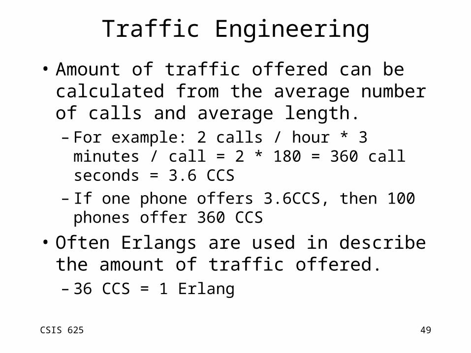
Traffic Engineering

• Amount of traffic offered can be calculated from the average number of calls and average length.– For example: 2 calls / hour * 3 minutes / call =

2 * 180 = 360 call seconds = 3.6 CCS– If one phone offers 3.6CCS, then 100 phones

offer 360 CCS

• Often Erlangs are used in describe the amount of traffic offered.– 36 CCS = 1 Erlang

CSIS 625 50

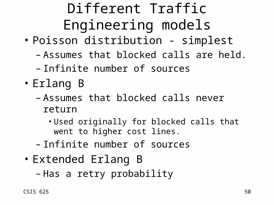
Different Traffic Engineering models

• Poisson distribution - simplest – Assumes that blocked calls are held.– Infinite number of sources

• Erlang B – Assumes that blocked calls never return

• Used originally for blocked calls that went to higher cost lines.

– Infinite number of sources

• Extended Erlang B– Has a retry probability

CSIS 625 51

Different Traffic Engineering models

• Erlang C– Assumes that blocked calls are delayed– Infinite number of sources– Used for Call Center applications

• “Trunks” are service people

• There are models for Finite number of sources, but they are used much less often.– Even if they should be used - people don’t

• Equations given are nice, but either look up tables, or calculators are really used.

CSIS 625 52

Poisson Distribution

• Poisson assumes that blocked calls wait forever.– This will tend to over estimate the number of

trunks needed– Equation for Poisson

• N = Number of events to occur in a unit time (Number of trunks)

• A = Average number of events occuring per unit time (Traffic in Erlangs)

CSIS 625 53

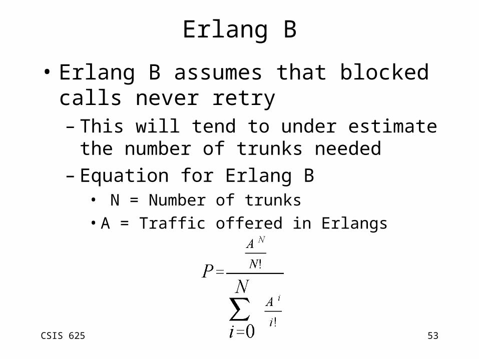
Erlang B

• Erlang B assumes that blocked calls never retry– This will tend to under estimate the number of

trunks needed– Equation for Erlang B

• N = Number of trunks

• A = Traffic offered in Erlangs

CSIS 625 54

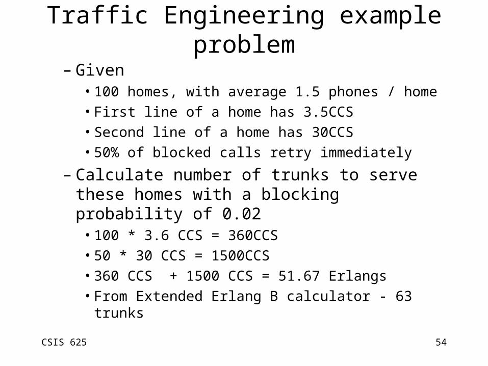
Traffic Engineering example problem

– Given • 100 homes, with average 1.5 phones / home

• First line of a home has 3.5CCS

• Second line of a home has 30CCS

• 50% of blocked calls retry immediately

– Calculate number of trunks to serve these homes with a blocking probability of 0.02

• 100 * 3.6 CCS = 360CCS

• 50 * 30 CCS = 1500CCS

• 360 CCS + 1500 CCS = 51.67 Erlangs

• From Extended Erlang B calculator - 63 trunks

CSIS 625 55

Traffic Engineering Web pages

– http://www.erlang.com/calculator/– http://www.owenduffy.com.au/electronics/

telecommunications.htm#Traffic modelling