CSIRO LAND and WATER

C S I R O L A N D a nd WAT E R

Application of the hypsometric integral and other terrain based

metrics as indicators of catchment health: A preliminary analysis

Trevor I. Dowling, D.P. Richardson, Aisling O’Sullivan,

Greg K. Summerell and Joe Walker

CSIRO Land and Water, CanberraTechnical Report 20/98, April 1998

Application of the hypsometric integral and other terrain basedmetrics as indicators of catchment health: A preliminaryanalysis

By Trevor I. Dowling, D. P. Richardson, Aisling O’Sullivan, Greg K. Summerelland Joe Walker.

CSIRO Land and Water, PO Box 1666, Canberra, ACT 2601 Australia.

Contact: T.I. DowlingCSIRO Water and LandPO Box 1666Canberra 2601+61 (02) 2465812 [email protected]

Technical Report No 20/98, April 1998

Copyright

© 2002 CSIRO Land and Water.To the extent permitted by law, all rights are reserved and no part of this publication covered bycopyright may be reproduced or copied in any form or by any means except with the writtenpermission of CSIRO Land and Water.

Important Disclaimer

To the extent permitted by law, CSIRO Land and Water (including its employees and consultants)excludes all liability to any person for any consequences, including but not limited to all losses,damages, costs, expenses and any other compensation, arising directly or indirectly from using thispublication (in part or in whole) and any information or material contained in it.

1

1. INTRODUCTION

This report documents the terrain analytical techniques and landscape metricsdeveloped as part of the project ‘Evaluating the success of tree planting fordegradation control’ (Walker et al., 1998a). The aims of the study were to assess theeffectiveness of farm scale tree plantings on landscapes, and in particular for salinitymanagement. It involved three phases:

1) A perception study – through landholder perceptions assess how well treesperform in land degradation control.

2) Measurement study – through field measurements, and guided by phase 1,check the accuracy of landholder perceptions in phase 1 and

3) Validation study – validate the conclusions from phases 1 and 2. Thevalidation study was further divided into:a) which species and how many trees are needed to have a measurable effect

on the targeted issueb) define ‘easy to use’ metrics or parameters to aggregate into an estimate of

catchment healthc) investigate landscape metrics useful in classifying catchments to assist

meaningful comparisons.

This report relates to phases 2 and 3 of the project and uses the National Tree Survey(NTS) data set which focused on small catchment sizes (100’s hectares), and theCatchment Health Study (CHS) data set which focused on large catchments (100000’s hectares). The purpose here is to:

- document the methods used to develop alternative indicators of catchment healthfor the NTS and CHS studies- investigate whether biophysical indicators could be used to quickly characterisecatchments with respect to susceptibility to dryland salinisation.

A central theme in developing terrain based indicators of catchment health is tobenchmark and monitor the condition of land and water resources within catchments(Walker and Reuter, 1996). Although essentially static, the topographiccharacteristics or morphometry of a catchment can have a substantial impact on how acatchment will respond to land use changes, relative to other catchments. Biophysicalcondition, the basic character of a catchment, together with land use managementcontrols key water quality degradation issues such as salinity, sedimentation andnutrient transport. Typical indicators of catchment health include stream electricalconductivity (EC), stream turbidity and tree cover. Although the broad aim of bothstudies was to assess the affect of tree cover on catchment health, this part aimed toexplore the contribution biophysical indicators could provide.

Several terrain based metrics were considered together with other data sources toexplore potential indicators of catchment health that could be easily acquired for anylocation in Australia. The main interest was in the hypsometric integral howeverseveral other metrics were used and investigated for their applicability to landscapefunction analysis and catchment characterisation studies.

2

This report describes an automated implementation of a hypsometric analysis forsmall size and large size catchments, and some observations of other metrics orindices that were investigated The emphasis is on fast and achievable estimates ratherthan definitive answers requiring large volumes of data and resources. The algorithmswere developed to run in the ArcInfo Geographic Information System (GIS).

Hypsometric, or area – altitude analysis, relates horizontal cross sectional area of adrainage basin to the relative elevation above the basin mouth, and was first describedby Strahler (1952). The hypsometric integral is appealing because it is adimensionless parameter and therefore allows different catchments to be comparedirrespective of scale. It integrates three dimensions, combining area on the x-axis withelevation on the y-axis. The result was described by Strahler as a measure of theerosional state or geomorphic age of the catchment. In theory hypsometric valuesrange from 0 to 1 (in this study the range was from 0.19 to 0.67). Low values areinterpreted by Strahler to represent old eroded landscapes, and high values as young,less eroded landscapes. The use of hypsometric analysis has been restricted in the pastbecause of the intensive computation required. Strahler acknowledged that for theeffort involved (using a planimeter) it would be more efficient to make a visualassessment of the contours. However, with the advances in computing and GIStechnology since 1952, hypsometry is worth reinvestigating as a means of objectivelyquantifying catchment characteristics

Other metrics investigated were circularity, catchment area and perimeter length.Circularity can be interpreted in terms of salinity hazard. That is, catchments thatapproach a circular shape are more likely to behave differently to long linearnetworks. They tend to be slow flowing, have depositional layers and low gradientsand more prone to salinisation. Linear catchments tend to have faster channeldrainage and are less prone to salinisation.

.

3

2. METHODS

2.1 General

The analyses are described in two parts. The first is an analysis of 47 catchments (6.8– 4,008 ha in area) that were studied as part of a National Tree Survey (NTS) (Walkeret al., 1998a). The second is an extension of the NTS called the Catchment HealthStudy (CHS) where 7 much larger pilot areas (48,000 – 663,000 ha.) were studied inconjunction with rapid survey techniques for assessing percentage tree cover, streamsalinity / turbidity and general health estimates.

Calculation of the hypsometric integral (i.e. the area under the hypsometric curve) wasautomated in ArcInfo Macro Language (AML) using the TOPOGRID and hydrologicfunctions available in GRID (ESRI 1995). A contour interval of 10m was chosen forboth analyses primarily because it was the input contour interval of the firstcatchments studied and allowed for direct comparison with manual planimetermethods. It also provided enough elevation ranges for the average relief to givesmooth hypsometric curves without compromising processing times. The latter isnormally the main criterion for the choice of contour interval.

The method, involving summing cells above contours, is very forgiving of poorquality data in that it will work with any DEM for any area and does not need to be adefined catchment. A hydrologically sound DEM is not critical, however, the qualityof the analysis is linked to the quality of the DEM therefore large errors are reflectedthe results accordingly.

Other catchment metrics, with potential to refine and add to the description andclassification while maintaining the simplicity and speed of the approach wereinvestigated. One method comparing area-perimeter ratios for catchments to that of acircle and is described.

A circularity index was calculated as follows:

area

perimieterycircularit

2

=

The circularity of a circle calculated in this way is 4πor 12.5. Similarly thecircularity of a square calculated in this way is 16.0.

Similar relationships were explored for rectangles and ellipses but are not reportedhere. Hypsometric and circularity indices were compared with stream electricalconductivity measurements at catchment outlets. This could be repeated on otherfactors, e.g. turbidity and subjective health classes or other indicators to test for furtherrelationships.

4

2.2 Data from the National Tree Survey (NTS): small catchments

The NTS aimed to assess the success of tree planting for the amelioration of landdegradation in heterogeneous landscapes. While the NTS was intended to haveNational application, the fieldwork was limited to 48 mainly first order catchments inNSW between Canberra, Wagga and Forbes. This was reduced to a subset of 14 siteswhere more reliable EC measurements taken in Creeks or gullies and (with theexception of 1 site) very low tree cover. EC, whilst easy to measure at a point, canvary greatly depending on the flow rate and volume of water in the streams and thetiming of the measurement. Reliability here refers to measurement times thatcoincided with low flows on the hydrograph. EC is taken as the indicator ofdegradation in this analysis.

Catchments were defined as the smallest complete watershed possible thatencompassed the tree lots being sampled, that is, down to a point on a watercoursewhere all drainage affected by the tree lot was accounted for. DEMs were notavailable at appropriate resolutions so a rapid method for generating DEMs wasdeveloped. They were derived using contours, streams and catchment boundariesdigitised from the best resolution maps available (usually 1:25000 or 1:50000) andinterpolated using ANUDEM (Hutchinson, 1989). A grid resolution of 20mx20m waschosen on the basis of manageability, appropriateness for the resolution of the inputdata and for the scale of the processes being measured in the overall study. Appendix1 is a summary of the process used in the NTS study to derive DEMs quickly fromminimal data. Appendix 2 is a listing of the automated hypsometric program whichconsists of three linked AMLs for accumulating cells between contours, processingthe resulting tables to derive required parameters and plotting the results.

2.2 Data from the Catchment Health Study (CHS): large catchments

This study focused on rapid sampling techniques for health assessment of largecatchments using spatially sparse but well selected sites that could be sampled morefrequently. The objective was to develop methods for monitoring catchment healthrelated characteristics that would require only 1 day per catchment (up to 500,000ha.). Measurements were taken for electrical conductivity (EC) and turbidity ofstreams, stream flow rate and trials of subjective health measures in the field. Variousmethods of obtaining percentage tree cover estimates from air photos or satelliteimagery were also tested in the laboratory and an order of precedence defined with airphotos preferred to satellite classifications and then field estimates.

An existing DEM was obtained for this work at 9 second or approximately 250mresolution (AUSLIG, 1997). This was the best available and appropriate for verylarge catchments. Catchment boundaries were obtained (CaLM, 1996) together withother ancillary coverages of hydrography, roads, place names etc from digital1:250000 topographic data series (AUSLIG, 1996). Hypsometric analysis andcalculation of the shape indices were performed in the same manner as the NTScatchments except that ancillary data was obtained separately or generated from the

5

DEM. These indices were compared with sampled EC measurements and tree coverestimated from available sources.

Appendix 2 lists the automated hypsometric program which is the same as that for theNTS in three linked AMLs.

3. RESULTS AND VISUALISATION:

Small catchments (NTS)

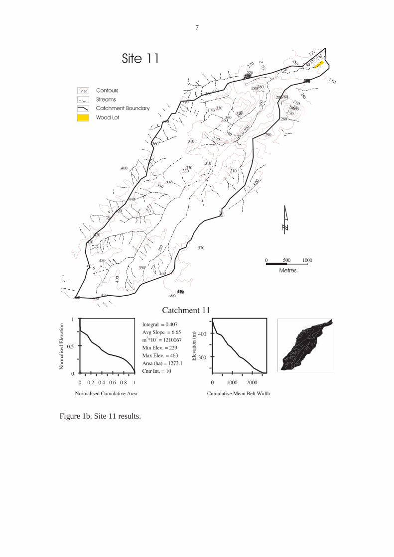
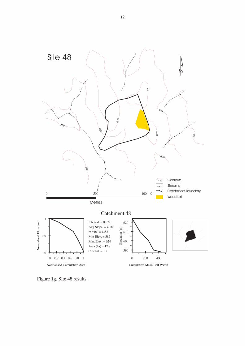
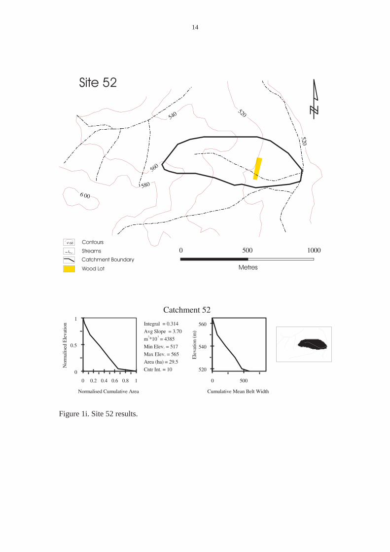
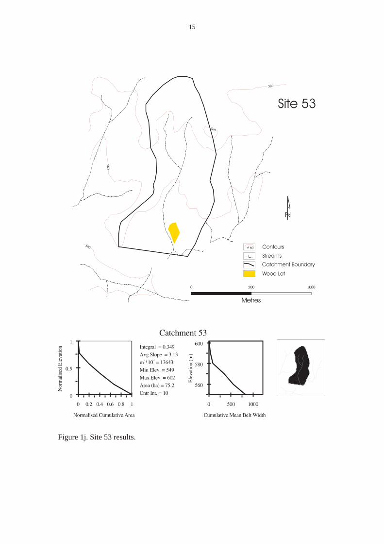
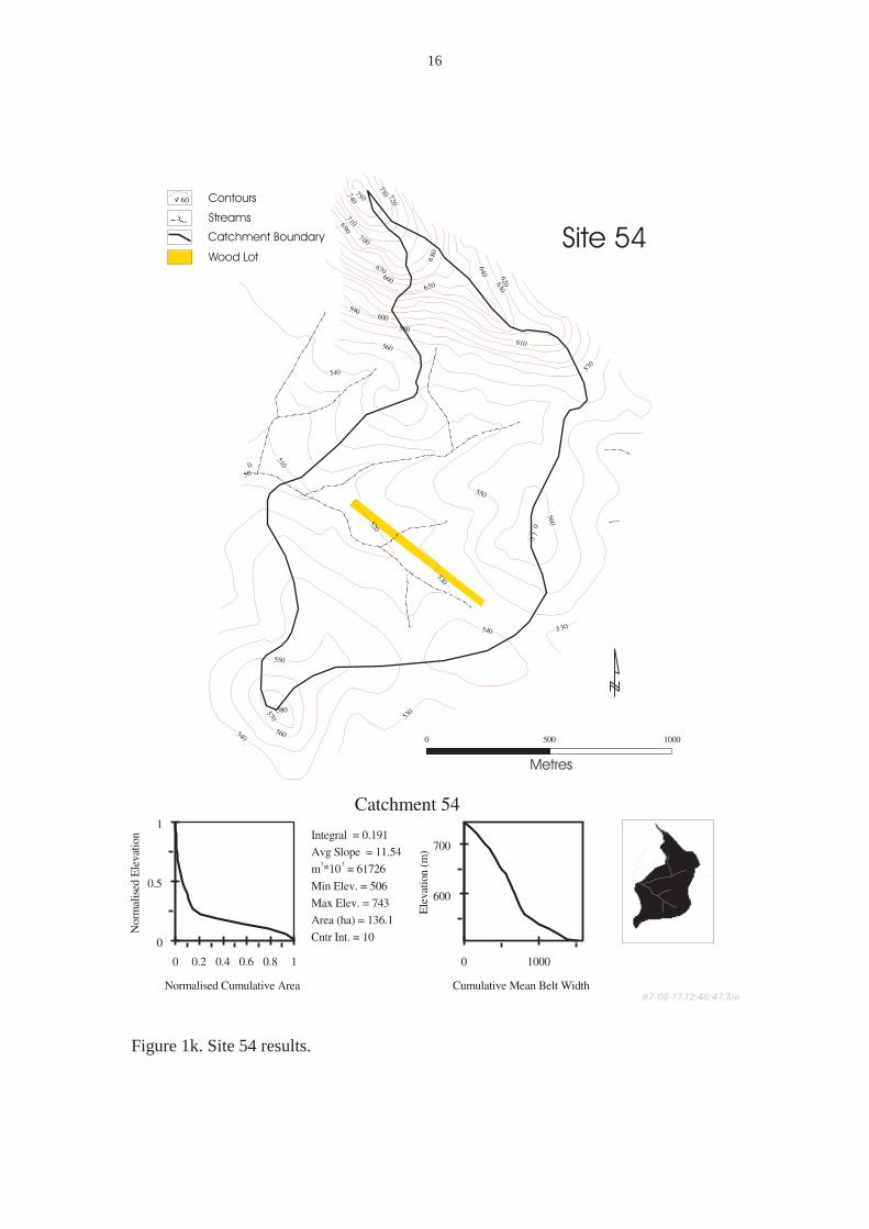
A typical site visualization and summary for an NTS catchment is presented in Figure1(a-n). It shows a site map of the digitised data in the upper portion of the page and asummary of results from the hypsometric analysis program in the lower portion. Thesummary includes:

1. the hypsometric curve;2. statistics for the catchment including integral (area under the curve), average

slope, volume under the curve, minimum and maximum elevations, area andcontour interval used;

3. a graph of the cumulative mean belt width (i.e. actual mean slope);4. a location map showing the context of the catchment relative to the extent of

the input data.

The hypsometric integrals for all the NTS catchments ranged from .180 to .672, with 1in the youthful phase, 30 in mature phase and 16 in very old phase. Table 1 showsresults for the 14 sites considered to have the most reliable EC measurements. Thesedata suggest that hypsometric integral is not related to any of the measures, especiallyEC. Some plots are given to illustrate the general lack of relationships (Figures 2 to6).

6

Figure 1a. Site 1 results.

Contours

Streams

Catchment Boundary

Wood Lot

Metres

Site 1

7

Figure 1b. Site 11 results.

Contours

Streams

Catchment Boundary

Wood Lot

Metres

Site 11

8

Figure 1c. Site 12 results

Contours

Streams

Catchment Boundary

Wood Lot

Metres

Site 12

9

Figure 1d. Site 21 results.

Contours

Streams

Catchment Boundary

Wood Lot

Site 21

Metres

10

Figure 1e. Site 23 results.

Contours

Streams

Catchment Boundary

Wood Lot

Site 23

Metres

11

Figure 1f. Site 40 results.

Contours

Streams

Catchment Boundary

Wood Lot

Site 40

Metres

12

Figure 1g. Site 48 results.

Contours

Streams

Catchment Boundary

Wood Lot

Site 48

Metres

13

Figure 1h. Site 50 results.

Contours

Streams

Catchment Boundary

Wood Lot

Site 50

Metres

14

Figure 1i. Site 52 results.

Contours

Streams

Catchment Boundary

Wood Lot

Site 52

Metres

15

Figure 1j. Site 53 results.

Contours

Streams

Catchment Boundary

Wood Lot

Metres

Site 53

16

Figure 1k. Site 54 results.

Contours

Streams

Catchment Boundary

Wood Lot

Site 54

Metres

17

Figure 1l. Site 55 results.

Contours

Streams

Catchment Boundary

Wood Lot

Metres

Site 55

18

Figure 1m. Site 62 results.

Contours

Streams

Catchment Boundary

Wood Lot

Site 62

Metres

19

Figure 1n. Site 65 results.

Contours

Streams

Catchment Boundary

Wood Lot

Site 65

Metres

20

SiteNo.

Hyps.Integral

Av. Slope(deg)

Area(ha.)

Perimeter(m)

Circularity MinElev

MaxElev

Treecover (%)

EC(us/cm)

48 .672 4.2 17.8 1,757.7 17.39 587 624 10 2300 g50 .535 3.1 199.9 6,843.6 23.46 574 643 2 1200 c12 .516 4.4 10.0 1,724.8 30.03 336 380 5 76 g62 .495 3.2 609.7 10,021.8 16.48 365 481 1 1776 c1 .480 7.2 6.8 1,615.3 37.30 399 474 90 79 g

65 .448 3.4 173.7 5,316.7 16.29 359 423 2 1300 c21 .425 4.3 60.4 3,101.3 15.91 348 404 1 3636 c55 .419 8.7 44.9 3,115.8 21.68 410 523 3 275 g11 .407 6.7 1273.0 19,858.3 30.98 229 463 1 779 c40 .402 1.6 109.2 4,362.5 17.47 455 501 1 558 g23 .355 3.9 94.8 4,371.7 20.14 376 471 3 2430 g53 .349 3.1 75.2 3,977.2 21.03 549 602 2 1300 g52 .314 3.7 29.5 2,405.5 19.73 517 565 2 1130 g54 .191 11.5 136.1 6,171.5 28.00 506 743 1 412 g

Range .492 11.2 4001.2 30,242.0 22.5 363 441 89 3560Mean .399 4.3 268.8 5,663.1 19.9 116 127 8.9 1232.2

Std Dev. .104 2.42 627.96 5,424.5 4.6 394 535 23.5 1022.2

Table 1. Summary for 14 small National Tree Survey Catchments after poor data andnon-creek (c) /gully (g) EC measurements were removed.

Figure 2. The hypsometric integral is not correlated with EC

Hypsometric Integral v's EC

y = 2083.5x2 - 161.95x + 892.97

R2 = 0.0347

0500

1000150020002500300035004000

0.1 0.2 0.3 0.4 0.5 0.6 0.7 0.8

Integral

EC

(us/

cm)

21

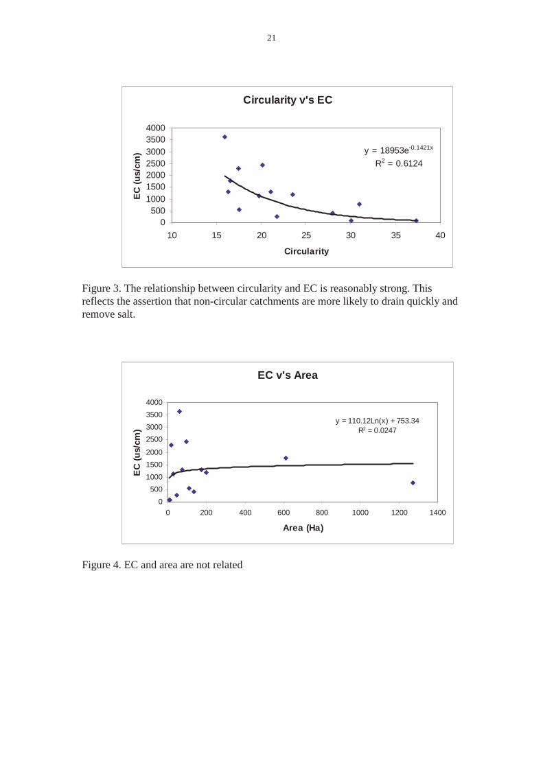
Figure 3. The relationship between circularity and EC is reasonably strong. Thisreflects the assertion that non-circular catchments are more likely to drain quickly andremove salt.

Figure 4. EC and area are not related

EC v's Area

y = 110.12Ln(x) + 753.34R2 = 0.0247

0

500

1000

1500

2000

2500

3000

3500

4000

0 200 400 600 800 1000 1200 1400

Area (Ha)

EC

(us/

cm)

Circularity v's EC

y = 18953e-0.1421x

R2 = 0.6124

0500

1000150020002500300035004000

10 15 20 25 30 35 40

Circularity

EC

(us/

cm)

22

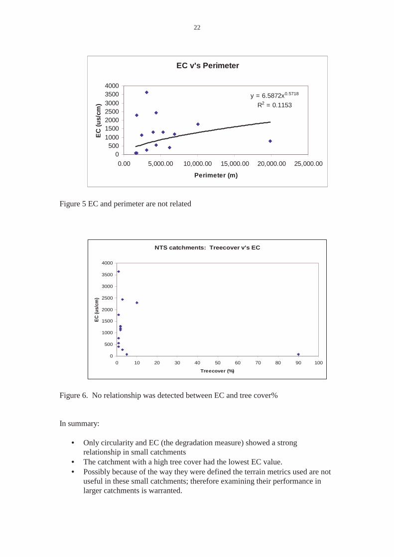
Figure 5 EC and perimeter are not related

Figure 6. No relationship was detected between EC and tree cover%

In summary:

• Only circularity and EC (the degradation measure) showed a strongrelationship in small catchments

• The catchment with a high tree cover had the lowest EC value.• Possibly because of the way they were defined the terrain metrics used are not

useful in these small catchments; therefore examining their performance inlarger catchments is warranted.

NTS catchments: Treecover v's EC

0

500

1000

1500

2000

2500

3000

3500

4000

0 10 20 30 40 50 60 70 80 90 100

Treecover (%)

EC

(us/

cm)

EC v's Perimeter

y = 6.5872x0.5718

R2 = 0.1153

0500

1000150020002500300035004000

0.00 5,000.00 10,000.00 15,000.00 20,000.00 25,000.00

Perimeter (m)

EC

(us/

cm)

23

• In addition EC measures are unreliable in small catchments because of thevery rapid decline in water flow.

• Tree cover some confounding effects on hypsometric relationships.

The 7 Large catchments (CHS)

The summaries and visualizations of the hypsometric analysis for the 7 large CHScatchments are given in Figure 7. Table 2 summarises the values for all the metricsfor the large catchments. The range of hypsometric integral values for the CHScatchments was .152 to .431 with 4 in the mature phase and 3 in the very old phase.Plots are given to illustrate the relationships between EC and metrics (Figures 8 to12).

25

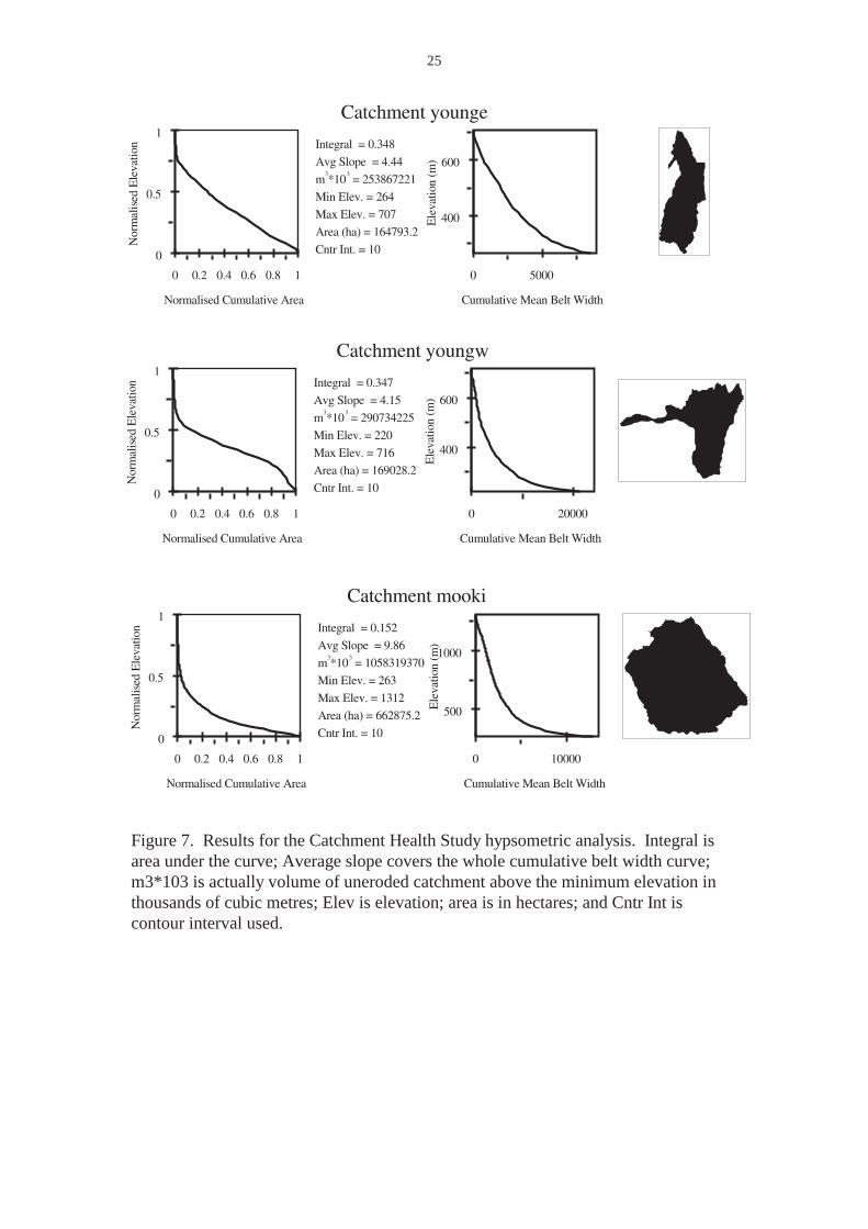
Figure 7. Results for the Catchment Health Study hypsometric analysis. Integral isarea under the curve; Average slope covers the whole cumulative belt width curve;m3*103 is actually volume of uneroded catchment above the minimum elevation inthousands of cubic metres; Elev is elevation; area is in hectares; and Cntr Int iscontour interval used.

26

Catchmentname

Hypso-metric

Integral

Averageslope(deg)

Area(ha)

(grid)

Perimeter( m )

Circularity( grid )

MinElev

MaxElev

TreeCoverest. %

TreeCoverest.

method

EC (us/cm)spatial mean

CHS pilot

EC (us/cm)at outlet

CHS pilot

Cotter 0.431 11.2 48,213 149,078 46.1 485 1,894 95.5 2,3,4 59 60

Jugiong 0.390 5.1 219,696 240,651 26.4 227 830 2.0 5 1731 1300

Queanbeyan 0.390 6.7 96,875 194,657 39.1 564 1,593 54.0 1,3 216 140

Yass 0.364 3.4 122,453 201,400 33.1 480 921 18.2 3,4 914 710

Young East 0.348 4.4 164,793 250,000 37.9 264 707 - 1,5 1145 1437

Young West 0.347 4.2 169,028 286,227 48.5 220 716 - 1,5 1584 1580

Mooki 0.152 9.9 662,875 371,223 20.8 263 1,312 15.0 1 1053 590

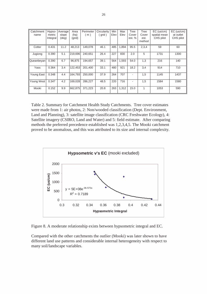
Table 2. Summary for Catchment Health Study Catchments. Tree cover estimateswere made from 1: air photos, 2: Non/wooded classification (Dept. Environment,Land and Planning), 3: satellite image classification (CRC Freshwater Ecology), 4:Satellite imagery (CSIRO, Land and Water) and 5: field estimate. After comparingmethods the preferred precedence established was 1,2,3,4,5. The Mooki catchmentproved to be anomalous, and this was attributed to its size and internal complexity.

Hypsometric v's EC (mooki excluded)

y = 5E+08e-36.573x

R2 = 0.7189

0

500

1000

1500

2000

0.3 0.32 0.34 0.36 0.38 0.4 0.42 0.44

Hypsometric Integral

EC

(us/

cm)

Figure 8. A moderate relationship exists between hypsometric integral and EC.

Compared with the other catchments the outlier (Mooki) was later shown to havedifferent land use patterns and considerable internal heterogeneity with respect tomany soil/landscape variables.

27

Circularity v's EC (mooki excluded)

y = 4810.6e-0.0583x

R2 = 0.11830

500

1000

1500

2000

0 10 20 30 40 50 60

Circularity Index

EC

(us/

cm)

Figure 9. At the larger scale circularity was not related to EC, yet it was correlated atthe small scale.

Area v's EC (mooki excluded)

y = 3E-10x2.4133

R2 = 0.8852

0

500

1000

1500

2000

2500

0 50,000 100,000 150,000 200,000 250,000

Area (ha)

EC

(us/

cm)

Figure 10. The relationship between catchment area and EC is strong

28

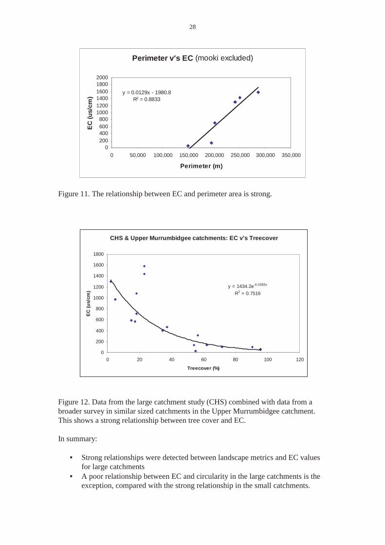
Perimeter v's EC (mooki excluded)

y = 0.0129x - 1980.8R2 = 0.8833

0200400600800

100012001400160018002000

0 50,000 100,000 150,000 200,000 250,000 300,000 350,000

Perimeter (m)

EC

(us/

cm)

Figure 11. The relationship between EC and perimeter area is strong.

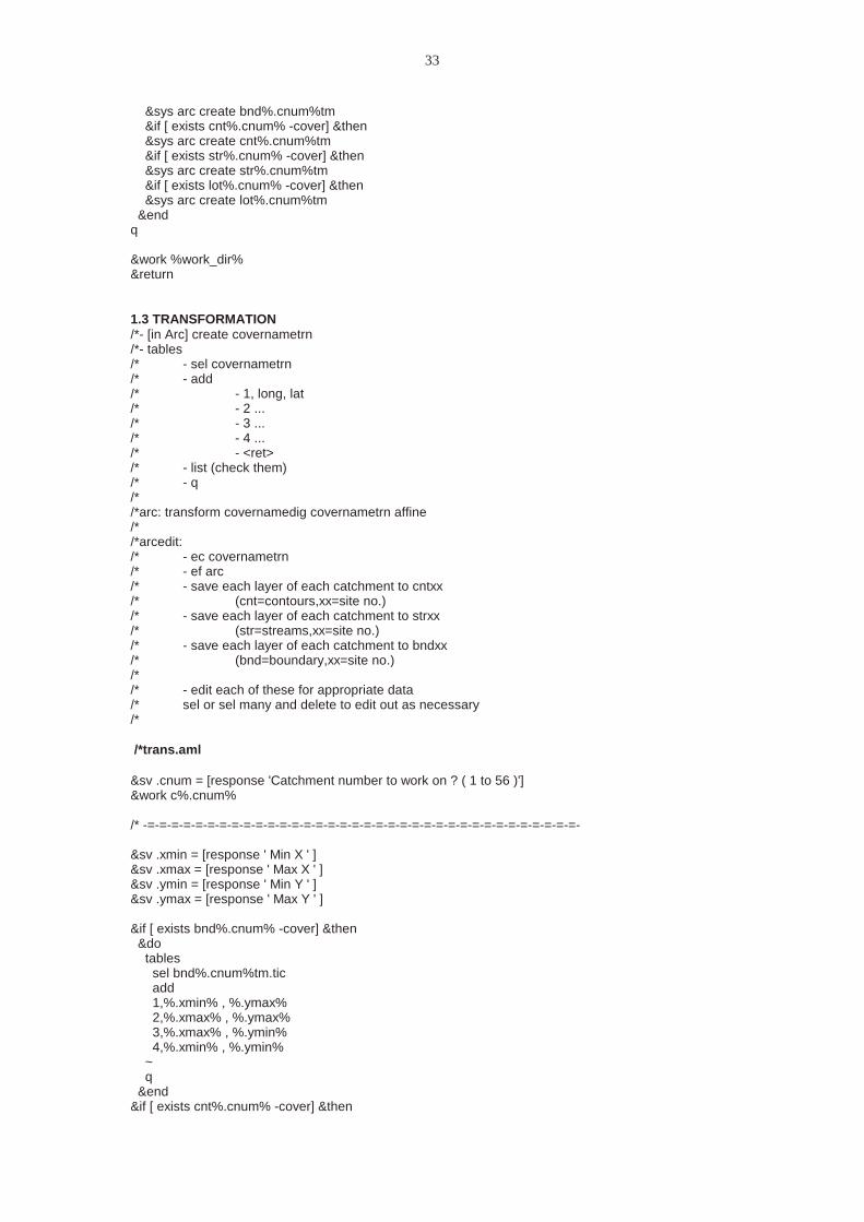
Figure 12. Data from the large catchment study (CHS) combined with data from abroader survey in similar sized catchments in the Upper Murrumbidgee catchment.This shows a strong relationship between tree cover and EC.

In summary:

• Strong relationships were detected between landscape metrics and EC valuesfor large catchments

• A poor relationship between EC and circularity in the large catchments is theexception, compared with the strong relationship in the small catchments.

CHS & Upper Murrumbidgee catchments: EC v's Treecover

y = 1434.2e-0.0355x

R2 = 0.7516

0

200

400

600

800

1000

1200

1400

1600

1800

0 20 40 60 80 100 120

Treecover (%)

EC

(us/

cm)

29

• The number of sites limits firm conclusions, but can be considered to be anencouragement for further sampling and analysis.

4. KEY MESSAGES

This paper documents preliminary research on several landscape metrics rarelyinvestigated quantitatively. It represents the beginning of a larger study to classifycatchments into different functional types and to apply biophysical indicators toestimate catchment health.

The hypsometric approach developed by Strahler and automated here has promise as aterrain analysis tool for:

• riparian studies (Prosser and Dowling, 1998),• erosion indices (Prosser and Gallant, unpublished),• indicators of catchment health (Walker et al., 1998b)• catchment classification / categorisation generally (Walker and Evans, 1997).• use as an ‘envelope’ as in the BIOCLIM type modeling that used climatic

envelopes for predicting the potential range of plants and animals (Nix, 1986;Busby, 1986)

The mmethods developed for rapidly determining the hypsometric integral forcatchments are useful where a DEM exists, but can be applied easily for smaller areaswhere only a contour map is available, with greater efficiency, flexibility and lesserror. Using a planimeter to measure small irregular areas was difficult.

Better correlations between EC and other indices existed in the larger catchmentsonly, suggesting a need to examine the field sampling method, the nature ofenvironmental signal attenuation and influences of areal scale. Sorting out thecomplex interactions between geomorphic underpinning and land use impacts,including tree planting, represents a major challenge.

For the larger CHS catchments, the removal of 1 outlier catchment resulted in strongrelationships between EC and most metrics.

The fact that we could easily identify an outlier suggests there may be a strongpotential for identifying anomalous catchments, and this could be useful forclassifying catchments into functional types.

Catchment classifications using single terrain attributes as indicators are unlikely tosucceed. Applying combinations of indicators in a framework such as anenvironmental envelope or an aggregated index are worth investigating.

30

References

AUSLIG (1996) Topo250k Digital Data, Auslig, Canberra, Australia

AUSLIG (1997) 9 second DEM, Auslig, Canberra, Australia

Busby, JR. (1986) Bioclimatic Prediction System (BIOCLIM) User's Manual Version2.0 Australian Biological Resources Study Leaflet.

CaLM, 1996) Water resources catchment boundaries, GIS Group, NSW Conservationand Land Management, Paramatta, Sydney, Australia.

ESRI (1995) ARC/INFO Users Guide, version 7.0, ESRI, California.

Hutchinson, MF. (1989). A new method for gridding elevation and stream line datawith automatic removal of pits. J. Hydrol. 106, 211232.

Nix, H.A. (1986) A biogeographic analysis of Australian Elapid Snakes. In. Atlas ofElapid Snakes of Australia. (ed.) R. Longmore pp. 415. Australian Flora and FaunaSeries Number 7. Australian Government Publishing Service: Canberra.

Prosser, I.P. and Dowling, T.I. (1997) Using catchment Morphology to Choose Whereto Locate Riparian Buffer Strips, 24th Hydrology and Water Resources Symposium,Auckland, November 1997, Institution of Engineers Australia, in press

Prosser, I.P., Dowling, T.I. and Rustomji, P. (1998) Catchment scale sedimentdelivery to streams: Linking process models, network structure and hillslopetopography. 8th Australian and New Zealand Geomorphology Conference, Nov. 15-20, 1998, Goolwa, South Australia.

Strahler, A.N. (1952) Hypsometric (area-altitude) analysis of erosional topography.Bulletin Geological Society of America, 1952, 63:1117-1142.

Walker, J., Dowling, T.I., Fitzgerald, W., Hatton, J., Mackenzie, D.H., Milloy, B.A.,Nicol, C.N., O’Sullivan, A. and Richardson, D.P. (1998a) Evaluating the Success oftree planting for degradation control. Final Report on the National Landcare Project.CSORO, Land and Water, Canberra, March 1998.

Walker, J., Jones, K.B., Dowling, T.I., Wickham, J.D., and Kepner, W. (1998b)Indicators of Landscape condition and Trends. Conference Paper, VII InternationalCongress of Ecology. Florence, Italy – 19/25 July 1998.

Walker, J. and Evans, W.R. (1997) National classification of catchments for land andriver salinity control. RIRDC National Workshop, Canberra, May 1997.

Walker, J. and Reuter, D.J. (1996) Key indicators to assess farm and catchmenthealth. In Indicators of catchment health – a technical perspective. [Walker, J andReuter, D Eds.], CSIRO Publishing, Australia.

31

APPENDIX 1. Summary of the Method of Processing NTS catchments

Documentation for deriving DEMs in the NTS topographic assessments:

NOTE: these data sets are intended as rapid assessments only.

T Dowling, CSIRO Div Water Resources, Canberra15.8.1996 - completion of the work up to and including the hypsometric analysis23.8.1996 – commencement date for this documentation.

Filename prefixes: bndnn - boundary for catchment ‘nn’cntnn - contours for catchment ‘nn’lotnn - tree lots in catchment ‘nn’strnn - streams in catchment ‘nn’

STEP 1.1:1:25000 or 50000 mapsheet -> _STARTDIG.AML -> bndnn

(& cntnn and lotnn and strnn)

STEP 1.2:Digitised covers -> GETMAP.AML -> copied to appropriate computer,

drawn to check,built appropriately

( (bndnn, cntnn, lotnn, strnn)

STEP 1.3:Built covers -> TRANS.AML -> asks for min’s & max’s, adds tics,

then transforms to AMG(bndnntm, cntnntm, lotnntm, strnntm )

digitising was quick and dirty - typical input/output RMS of .003/5.some, like on the corner of 4 sheets as bad as .1/11.this wasn't seen as critical for this 'quick look method' and shouldn'tbe used for anything where high accuracy is important.

STEP 1.4:transformed covers -> TOPO.AML -> DEM, masks catchment

(demnn, masknn, catnn)

STEP 2: Ready to invoke hmetric.aml (see Appendix 2)Masked DEM -> HMETRIC.AML -> hypsometric calculations for catchment

(hypnn.tbl)

32

APPENDIX 1. (cont) Detailed listings of AML’s used in NTS process.

1.1 Digitising:

run _STARTDIG- digitise tics ( MAP CORNERS, NOTE LONG/LATS for transform later)- digitise two world points outside map area (aml requirement)- digitise catch boundaires (ie with auto increment from 1 [default])- digitise streams following straight on- digitise contours BUT change id each time to that of contour value

needs 8 (to get menu up )needs 1 (to set id using cursor numbers)needs A (to enter number)needs 2 (to start line)needs 1 (for vertices)needs 2 (to end line)

repeat for all contours

1.2 Copying files from digitising computer to appropriate working directory if necessaryGetmap.aml:

&work %work_dir%&sv grd = [response 'Are we already in GRID ? ( y or n )']&if %grd% ne 'y' and %grd% ne 'Y' &then

&dogrid

&endclearunits map

&sv .cnum = [response 'Catchment number to work on ? ( 1 to 56 )']

&if not [ exists c%.cnum% -directory] &then&sys mkdir c%.cnum%

&work c%.cnum%&if [ exists %dig_dir%/bnd%.cnum% -cover] &then&sys arc copy %dig_dir%/bnd%.cnum% bnd%.cnum%&if [ exists %dig_dir%/cnt%.cnum% -cover] &then&sys arc copy %dig_dir%/cnt%.cnum% cnt%.cnum%&if [ exists %dig_dir%/str%.cnum% -cover] &then&sys arc copy %dig_dir%/str%.cnum% str%.cnum%&if [ exists %dig_dir%/lot%.cnum% -cover] &then&sys arc copy %dig_dir%/lot%.cnum% lot%.cnum%&sys arc lc

mape cnt%.cnum%linecolor orange&if [ exists cnt%.cnum% -cover] &thenarcs cnt%.cnum%linecolor blue&if [ exists str%.cnum% -cover] &thenarcs str%.cnum%linecolor red&if [ exists bnd%.cnum% -cover] &thenarcs bnd%.cnum%linecolor green&if [ exists lot%.cnum% -cover] &thenarcs lot%.cnum%

&sv ok = [response 'Ready to work on ? ( GRID will exit )']&if %ok% eq 'y' or %ok% eq 'Y' &then

&do&if [ exists bnd%.cnum% -cover] &then

33

&sys arc create bnd%.cnum%tm&if [ exists cnt%.cnum% -cover] &then&sys arc create cnt%.cnum%tm&if [ exists str%.cnum% -cover] &then&sys arc create str%.cnum%tm&if [ exists lot%.cnum% -cover] &then&sys arc create lot%.cnum%tm

&endq

&work %work_dir%&return

1.3 TRANSFORMATION/*- [in Arc] create covernametrn/*- tables/* - sel covernametrn/* - add/* - 1, long, lat/* - 2 .../* - 3 .../* - 4 .../* - <ret>/* - list (check them)/* - q/*/*arc: transform covernamedig covernametrn affine/*/*arcedit:/* - ec covernametrn/* - ef arc/* - save each layer of each catchment to cntxx/* (cnt=contours,xx=site no.)/* - save each layer of each catchment to strxx/* (str=streams,xx=site no.)/* - save each layer of each catchment to bndxx/* (bnd=boundary,xx=site no.)/*/* - edit each of these for appropriate data/* sel or sel many and delete to edit out as necessary/*

/*trans.aml

&sv .cnum = [response 'Catchment number to work on ? ( 1 to 56 )']&work c%.cnum%

/* -=-=-=-=-=-=-=-=-=-=-=-=-=-=-=-=-=-=-=-=-=-=-=-=-=-=-=-=-=-=-=-=-=-=-=-=-

&sv .xmin = [response ' Min X ' ]&sv .xmax = [response ' Max X ' ]&sv .ymin = [response ' Min Y ' ]&sv .ymax = [response ' Max Y ' ]

&if [ exists bnd%.cnum% -cover] &then&do

tablessel bnd%.cnum%tm.ticadd1,%.xmin% , %.ymax%2,%.xmax% , %.ymax%3,%.xmax% , %.ymin%4,%.xmin% , %.ymin%

~q

&end&if [ exists cnt%.cnum% -cover] &then

34

&dotables

sel cnt%.cnum%tm.ticadd1,%.xmin% , %.ymax%2,%.xmax% , %.ymax%3,%.xmax% , %.ymin%4,%.xmin% , %.ymin%

~q

&end

&if [ exists str%.cnum% -cover] &then&do

tablessel str%.cnum%tm.ticadd1,%.xmin% , %.ymax%2,%.xmax% , %.ymax%3,%.xmax% , %.ymin%4,%.xmin% , %.ymin%

~q

&end

&if [ exists lot%.cnum% -cover] &then&do

tablessel lot%.cnum%tm.ticadd1,%.xmin% , %.ymax%2,%.xmax% , %.ymax%3,%.xmax% , %.ymin%4,%.xmin% , %.ymin%

~q

&end

&if [ exists bnd%.cnum%tm -cover] &then&do

&sys arc transform bnd%.cnum% bnd%.cnum%tm affine&sys arc build bnd%.cnum%tm poly

&end&if [ exists cnt%.cnum%tm -cover] &then

&do&sys arc transform cnt%.cnum% cnt%.cnum%tm affine&sys arc build cnt%.cnum%tm line

&end&if [ exists str%.cnum%tm -cover] &then

&do&sys arc transform str%.cnum% str%.cnum%tm affine&sys arc build str%.cnum%tm line

&end&if [ exists lot%.cnum%tm -cover] &then

&do&sys arc transform lot%.cnum% lot%.cnum%tm affine&sys arc build lot%.cnum%tm poly

&end

&work %work_dir%&return

1.4 topo2.aml/* Generate a DEM in TOPOGRID

&work %work_dir%&sv .cnum = [response 'Catchment number to work on ? ( 1 to 56 )']

35

&work c%.cnum%shadeset rainbow

&if [ exists dem%.cnum% -grid] &thenkill dem%.cnum% all

/*&if [ exists cat%.cnum% -grid] &then/* kill cat%.cnum% all

&if [ exists drn%.cnum% -cover] &thenkill drn%.cnum% all

&if [ exists drn20 -cover] &thenkill drn20 all

&if [ exists snk%.cnum% -cover] &thenkill snk%.cnum% all

&if [ exists snk20 -cover] &thenkill snk20 all

&if [ exists cnt%.cnum% -cover] &thenkill cnt%.cnum% all

&if [ exists cnt%.cnum%tm -cover] &thenkill cnt%.cnum%tm all

&if [ exists diagtm -file] &then&sys rm diagtm

&if [ exists diag20tm -file] &then&sys rm diag20tm

copy ../c71/dem71 dem%.cnum%copy ../c71/drn71 drn%.cnum%copy ../c71/snk71 snk%.cnum%

&sys cp -p ../c71/diagtm .

copy ../c71/cnt71 cnt%.cnum%copy ../c71/cnt71tm cnt%.cnum%tm

mape dem%.cnum%grids dem%.cnum% # linear nowrap

/*setcell dem%.cnum%/*setwindow bnd%.cnum%tm/*mask%.cnum% = polygrid ( bnd%.cnum%tm )

/*cat%.cnum% = con( mask%.cnum% gt 0, dem%.cnum%, setnull(1) )

grids cat%.cnum% # linear nowraplinecolor orange&if [ exists cnt%.cnum%tm -cover] &then

arcs cnt%.cnum%tmlinecolor blue&if [ exists str%.cnum%tm -cover] &thenarcs str%.cnum%tmlinecolor red&if [ exists bnd%.cnum%tm -cover] &thenarcs bnd%.cnum%tmlinecolor green&if [ exists lot%.cnum%tm -cover] &thenarcs lot%.cnum%tm

&sv ok = [response 'Exit GRID ( n to stay & run hmetric.aml ) ?']&if %ok% eq 'y' or %ok% eq 'Y' &then

&doq

&end&work ..show work&return

36

APPENDIX 2. AML scripts for processing catchment Hypsometrics

Appendix 2.1

/* HMETRIC3v2.AML/* written 16.04.97 ... tid/* to calculate hypsometric curves and call appropriate aml's to plot:/* addtab2v0.aml - takes tabluar output and installs in info table/* gtab2v0.aml - takes table and plots graph and location map/* modified 24.04.97 ... tid/* changed to accept and extract from a multi-item grid instead of/* choices of single ones/* copied to nts/catch/hmetric3v1 prior to 14.6.97; rerun for CHS June writeup/* copied to nts/catch/hmetric3v2 prior to 14.6.97; rerun for CHS June writeup/* modified 16.6.97 ... tid to reflect changes in ~/catch/hmetric3v0.aml,/* addtab2v0.aml/* gtab2v0.aml and/* gtabsum3.aml

&messages &off &info/* set up plotting environment – page layout

shadecolor cmy 0 0 0shadeput 257gridnodatasymbol 257textset font.txttextsymbol 1

&sv .nperpage = 4/*&sv .nperpage = 1&sv .nplt = 0&sv .npage = 0&sv .end = .FALSE.

&sv .ci = [response ' Contour interval [10]' 10 ]

/*&sv runopt = [response '[t]able with headers or (g)raph for ArcInfo' t]/* table is for exporting to excel graph is for graphical output to plot.&sv runopt = g

/* Select the catchment number to process ...&ty&ty Choose the set to analyse from -&ty&ty 0. all NTS catchments&ty 1. specific NTS / CHS catchment(s)&sv setopt = [response ' Option [1]' 1 ]

&if %setopt% eq 0 &then&do

/* could automate this with listunique…&sv nums =1,3,5,8,11,12,13,14,15,16,17,19,20,21,23,24,25,28,31,34,35,36,37,38,39,40,42,43,44,46,48,49,50,52,53,54,55,56,57,61,62,63,65,66,67,68,71

&end&else

&do&sv nums := [response ' Catchment number for this run (1 to 56)' ]

&end

&do .cnum &list %nums%

&work %work_dir%/c%.cnum%mape cat%.cnum%setwindow cat%.cnum%&sv geodataset = cat%.cnum%

37

&sv .outf = hmetric%.cnum%&sv outfil := %.outf%.tbl

&ty %outfil% %.cnum% : %nums%&sv i = [close -all]&if [ exists %outfil% ] &then

&do/* &sv resp = [response 'Delete this file ?' n]

&sv resp = y&if resp eq 'y' or resp eq 'Y' &then

&do&ty&ty rm'ing %outfil%&sys rm %outfil%

&end&end

&sv file_unit = [open %outfil% openstatus -write]&ty open status = %openstatus% (0 = OK)

&sv .catgrd = cat%.cnum%&sv slpgrd = slp%.cnum%&if [exists slp%.cnum% -grid] &then

kill slp%.cnum% allslp%.cnum% = slope ( cat%.cnum% )describe slp%.cnum%

/* &if [exists %.catgrd% -grid] &then kill %.catgrd% all/* %.catgrd% = con ( %geodataset% eq %.cnum%, fil5 )

shadeset rainbow

&if ^ [exists pol%.cnum% -grid] &thenpol%.cnum% = gridpoly ( msk%.cnum% )setwindow pol%.cnum%

/* Extract vital parameters from the grid ...

&describe %.catgrd%

&sv celldim = %GRD$DX%&sv dz = %GRD$ZMAX% - %GRD$ZMIN%

&sv .zmin = [truncate %GRD$ZMIN%]&sv diffmin = [mod %.zmin%, %.ci%]&sv mincntr = %.ci% - %diffmin% + %.zmin%

&sv .zmax = [round %GRD$ZMAX%]&sv diffmax = [mod %.zmax%, %.ci%]&sv maxcntr = %.ci% - %diffmax% + %.zmax%

&sv cntr1 = %mincntr% - %.ci%&sv cntrn = %maxcntr%

&sv cumarea = 0

/* Extract vital parameters from the grid ...

totcell = scalar (0)docell

{if ( %.catgrd% ge 0 )begin

totcell = totcell + 1end

}end

/* convert scalar to variables and prefix with a ‘v’stotcell = scalar (totcell )

&sv vtotcell = [show stotcell]

38

stotarea = scalar (totcell * %celldim% * %celldim% / 10000 )&sv .vtotarea = [show stotarea]

&if %runopt% eq t or %runopt% eq T &then&do

/* write out :catchment no, contour interval, Tot Area, Tot No cells,/* Zmin, Zmax, Relief

&sv recrd = [quote %.cnum% %.ci% %.vtotarea% %vtotcell% %GRD$ZMIN% %GRD$ZMAX% %dz% 00]

&if [write %file_unit% %recrd%] = 0 &then&do

&ty record written to %outfil%&end

&else&ty EMERGENCY ! file not written ...

&sv recrd = ' '&if [write %file_unit% %recrd%] = 0 &then

&do&ty Blank Separator record ...&ty record written to %outfil%

&end&else

&ty EMERGENCY ! file not written ...&end

/********************************************************************/* Iterate through the contour ranges and count matching cells off/* the grid ...

&sv .cum_belt = 0&sv .cum_vol = 0&sv .totcumbelt = 0&sv .avg_tot_slp = 0&sv n_intvl = 0

&do xxx = %cntr1% &to %cntrn% &by %.ci%&sv yyy = %xxx% + %.ci%

&if %xxx% lt %GRD$ZMIN% &then&sv .xxxtmp = %GRD$ZMIN%

&else &if %xxx% gt %GRD$ZMAX% &then&sv .xxxtmp = %GRD$ZMAX%

&else&sv .xxxtmp = %xxx%

&if %yyy% gt %GRD$ZMAX% &then&sv yyytmp = %GRD$ZMAX%

&else&sv yyytmp = %yyy%

&ty Processing area: %.cnum% %.xxxtmp% to %yyytmp% of %.zmin% to %.zmax%

mape %.catgrd%setcell %.catgrd%setwindow %.catgrd%

p1 = scalar(0.0)cumslp = scalar(0.0)ncells = scalar(0.0)cisclr = scalar ( %.ci% )

docell{

if ( %.catgrd% ge %.xxxtmp% and %.catgrd% lt %yyytmp%)begin

p1 = p1 + %.catgrd%

39

cumslp += %slpgrd%ncells = ncells + 1

end}

end /* end docell

/* Extract required stats from the accumulations .../* convert scalar to variables and prefix with a ‘v’

&sv n_intvl = %n_intvl% + 1

&sv v1 = [show p1]

&sv vncells = [show ncells]&sv .range = [ calc %yyytmp% - %.xxxtmp%]

&if ( %vncells% le 0 ) &then&do

avg_elev = scalar( (%.xxxtmp% + %yyytmp%) / 2 )avg_slp = scalar( 0 )avg_belt = scalar( 0 )sarea = scalar( 0 )

&end&else

&doavg_elev = scalar( p1 / ncells )avg_slp = scalar( cumslp / ncells )avg_belt = scalar( %.range% / [tan [angrad [show avg_slp]]] )sarea = scalar( ncells * %celldim% * %celldim% / 10000 )&sv area_m2 = [calc %vncells% * ( %celldim% * %celldim% )]

&end

&sv vavg_slp = [show avg_slp]&ty Avg_slp = %vavg_slp%

/* next bit is an accumulation and is averaged after the loop&sv .avg_tot_slp = %.avg_tot_slp% + %vavg_slp%&sv vavg_belt = [show avg_belt]&sv .cum_belt = %.cum_belt% + %vavg_belt%

&sv vavg_elev = [show avg_elev]&sv area = [show sarea]&sv cumarea = %cumarea% + %area%&sv invcumarea = %.vtotarea% - %cumarea% + %area%

&if %.vtotarea% gt 0 &then&sv nmlarea = %invcumarea% / %.vtotarea%

&else&sv nmlarea = 0&sv nmlxxx = ( %.xxxtmp% - %GRD$ZMIN% ) / %dz%

&sv nmlyyy = ( %yyytmp% - %GRD$ZMIN% ) / %dz%&sv nmlrange = [calc %nmlyyy% - %nmlxxx%]

/* write out : LOWER cntr (/elev), normalised LOWER cntr (/elev),/* avge elevation, No. cells, Area (Ha.), Cum. Area (Ha),/* Actual Inv. Cum. Area, Normalised Inv. Cum. Area,/* Range, Normalised range

&sv recrd = [quote %.xxxtmp% %nmlxxx% %vavg_elev% %vncells% %area% %cumarea%%invcumarea% %nmlarea% %.range% %nmlrange% %vavg_belt% %.cum_belt% %vavg_slp% ]

&if [write %file_unit% %recrd%] = 0 &then&sv errcode = 0

&else&ty EMERGENCY ! file not written ...

&end /* &do end

40

/*###################################################################

&sv .avg_tot_slp = %.avg_tot_slp% / [ calc %n_intvl% - 1 ]&ty %.avg_tot_slp%

setwindow cat%.cnum%

&r %PROG_DIR%/addtab2v0

&sv .nplt = [ calc %.nplt% + 1 ]&r %PROG_DIR%/gtab3v1

&if %.nplt% eq %.nperpage% &then&do

&sv .nplt = 0&sv .npage = %.npage% + 1

&end

/*###################################################################&end /* end &do &list/*###################################################################

/* allow for unplotted unfinished page of multiple plots&if %.nplt% gt 0 &then

&do&sv .end = .TRUE.&r %PROG_DIR%/gtab3v1

&end

/*###################################################################

&if %runopt% eq t &then&do

/* End of processing so close files and 'UNIX2DOS' it ready for /*Excel/Lotus ...

&if [close %file_unit% ] = 0 &then&do

&ty Output file closed&ty Converting %outfil% to DOS ...&sys mv %outfil% htmp&sys unix2dos htmp %outfil%

&end&else

&ty EMERGENCY ! file not closed ...&end

&messages &on&work %WORK_DIR%

&return

41

Appendix 2.2

/***********************************************************************************************************/* ADDTAB2v0.aml/***********************************************************************************************************/* variables read in from hmetric3v0:/* base contour/* Normalised Elevation/* Average Elevation/* No. of cells/* Area in Ha/* Cum Area in Ha/* Act. Inv. Cum Area/* Normalised Inv. Cum Area/* Range (=ci except at extremities)/* Avg contour-belt width for true mean slope curve

&sv .inptab := %.outf%.tbl&sv .outinf := %.outf%.tab&sv .cum_vol = 0

arc tables&if [exists %.outinf% -INFO] &then

&dosel %.outinf%erase %.outinf%

y&end

define %.outinf%base_ctr88N2nml_elev88N4avg_elev88N2n_cells1010iarea_ha1010N1cum_area1212N1inv_cum_area1212N1nml_inv_c_a88

42

N4range66N2nmlrange99N6avg_belt99N2cum_belt1212N2avg_slp88N4~

add base_ctr nml_elev avg_elev n_cells area_ha cum_area inv_cum_area nml_inv_c_a rangenmlrange avg_belt cum_belt avg_slp from %.inptab%seladditem %.outinf% invcumbelt 12 12 n 1additem %.outinf% avgarea 12 12 n 1additem %.outinf% nml_avg_a 8 8 n 5additem %.outinf% integral 8 8 n 6q

resel %.outinf% infonsel %.outinf% infocursor x0 declare %.outinf% info rwcursor x0 open

resel %.outinf% infonsel %.outinf% infocursor x1 declare %.outinf% info rocursor x1 open

resel %.outinf% infonsel %.outinf% infocursor x3 declare %.outinf% info rocursor x3 open&sv listrec = show listselect

&sv count = 0&sv backcount = 0&sv .integral = 0

&do &while %:x3.aml$next% ne .FALSE.cursor x3 next&sv backcount = [ calc %backcount% + 1 ]

&end

cursor x3 %backcount%&sv .totcumbelt = %:x3.cum_belt%&ty BACKCOUNT = %backcount% %.totcumbelt%&sv backcount = %backcount% + 1

43

&label loop

&if %:x0.aml$next% ne .FALSE. &then&do

&sv count = %count% + 1&sv backcount = %backcount% - 1

&if %count% ne 1 &then&do

cursor x0 next&if %backcount% gt 0 &then cursor x3 %backcount%

&end

&if %:x0.aml$next% eq .true. &then&do

cursor x1 next&ty %backcount% %:x3.cum_belt%&sv :x0.invcumbelt = %.totcumbelt% - %:x0.cum_belt%&sv :x0.avgarea = [calc [calc %:x0.inv_cum_area% + %:x1.inv_cum_area% ] / 2. ]&sv :x0.nml_avg_a = [calc [calc %:x0.nml_inv_c_a% + %:x1.nml_inv_c_a% ] / 2. ]&sv .integral = %.integral% + [calc %:x0.nml_avg_a% * %:x0.nmlrange% ]&sv :x0.integral = %.integral%

/* in next bit avgarea(ha) * 10000 to m2 / 1000 to ooo's m2 i.e. * 10&sv .cum_vol = %.cum_vol% + [calc %:x0.avgarea% * 10 * ~

%:x0.range% ]&end

&else&do

/* &sv :x0.invcumbelt = 0&ty %backcount% %:x0.cum_belt%&sv :x0.invcumbelt = %.totcumbelt% - %:x0.cum_belt%&sv :x0.avgarea = [calc [calc %:x0.inv_cum_area% + 0. ] / 2. ]&sv :x0.nml_avg_a = [calc [calc %:x0.nml_inv_c_a% + 0. ] / 2.]&sv .integral = %.integral% + [calc %:x0.nml_avg_a% * ~

%:x0.nmlrange% ]&sv :x0.integral = %.integral%

/* in next bit avgarea(ha) * 10000 to m2 / 1000 to ooo's m2 i.e. * 10&sv .cum_vol = %.cum_vol% + [calc %:x0.avgarea% * 10 * ~

%:x0.range% ]&end

&goto loop&end /* do while

cursor x0 closecursor x1 closecursor x3 close

cursor x0 removecursor x1 removecursor x3 remove

&return

44

Appendix 2.3

/********************************************************************/* GTAB3v1.aml/********************************************************************

/* written ... tid CSIRO, Land and Water/* modified .. 29.04.97 ... tid - created 2v1 from 2v0/* ... added capability for 3 plots to a page/* modified .. 17.06.97 ... tid - created 3v1 from ~/catch/3v0/* ... mods to fit CHS catchments/*

/* set variables&sv rundate = [ date -tag ]&sv outfil = gtab%.npage%%rundate%

units pagetextset fonttextsymbol 14textquality proportionaltextsize 10 pttextstyle typeset

/* check global variables have been passed OK&ty GTAB3v1: .nperpage %.nperpage% and .nplt %.nplt%

&if %.end% eq .FALSE. &then&do

&if %.nperpage% eq 1 &then&do

display 1040%outfil%.gra

/* graphlimits&sv glimx0 = 6.0&sv glimx1 = 16.0&sv glimy0 = 16.5&sv glimy1 = 26.5

/*maplimits&sv mlimx0 = 5.25&sv mlimx1 = 17.25&sv mlimy0 = 2.0&sv mlimy1 = 14.5

&end

&else &if %.nperpage% eq 4 &then&do

&sv gxcen = 5&sv g2xcen = 13.5&sv g_dy = 3.5&sv mxcen = 17.75&sv m_dy = 4

&if %.nplt% eq 1 &then&do

display 1040%outfil%.gra

&sv glimx0 = %gxcen% - [calc %g_dy% / 2 ]&sv glimx1 = %gxcen% + [calc %g_dy% / 2 ]&sv g2limx0 = %g2xcen% - [calc %g_dy% / 2 ]&sv g2limx1 = %g2xcen% + [calc %g_dy% / 2 ]&sv gycen = 25.5&sv glimy0 = %gycen% - [calc %g_dy% / 2 ]&sv glimy1 = %gycen% + [calc %g_dy% / 2 ]

/*maplimits

45

&sv mlimx0 = %mxcen% - [calc %m_dy% / 2 ]&sv mlimx1 = %mxcen% + [calc %m_dy% / 2 ]&sv mlimy0 = %gycen% - [calc %m_dy% / 2 ]&sv mlimy1 = %gycen% + [calc %m_dy% / 2 ]

&end



/*maplimits&sv mlimx0 = %mxcen% - [calc %m_dy% / 2 ]&sv mlimx1 = %mxcen% + [calc %m_dy% / 2 ]&sv mlimy0 = %gycen% - [calc %m_dy% / 2 ]&sv mlimy1 = %gycen% + [calc %m_dy% / 2 ]

&end




&end




&end&end

&sv inptab := %.outinf%

textcolor black/* &sv title1 := [quote Catchment %.cnum% ]

&sv title1 := [quote Catchment %.cnum% ]

clipgraphextent onpageunits cmpagesize 21 29.7

/* GRAPH 1 :

graphextent 0.0 0.0 1.0 1.0

46

lineset color.lintextsize 10 pt

/*linetype wide

graphlimits %glimx0% %glimy0% %glimx1% %glimy1%linecolor black

/* linecolor purplelinesize .05units pagebox [show graphlimits]

units graphlinesize .06axis horizaxisruler 'Normalised Cumulative Area'

axis verticalaxisruler

linesize .075markersize 0.1linecolor blackmarkercolor redgraphline %inptab% info nml_inv_c_a nml_elev

units pagelinesize .06textangle 90move [calc %glimx0% - 1.25] [calc %glimy0% + ( %glimy1% - ~

%glimy0% ) / 2 ]text 'Normalised Elevation' cctextangle 0

/* GRAPH 2 :

graphextent 0.0 %GRD$ZMIN% %.totcumbelt% %GRD$ZMAX%lineset color.lintextsize 10 pt

graphlimits %g2limx0% %glimy0% %g2limx1% %glimy1%linecolor blacklinesize .06units pagebox [show graphlimits]

units graphlinesize .06axis horizaxisruler 'Cumulative Mean Belt Width'

axis verticalaxisruler

linesize .075markersize 0.1linecolor blackmarkercolor redgraphline %inptab% info invcumbelt base_ctr

units page

linesize .06textangle 90move [calc %g2limx0% - 1.25] [calc %glimy0% + ( %glimy1% - ~

/* %glimy0% ) / 2 ]text 'Elevation (m)' cctextangle 0

47

&sv dxtext = 0.5&sv dytext = .5

move [calc %glimx1% + %dxtext% ] [calc %glimy1% - 2 * %dytext% ]&sv labpos = [search %.avg_tot_slp% .]&if %labpos% gt 0 &then

&sv labsub = [substr %.avg_tot_slp% 1 [calc %labpos% + 2 ] ]&else

&sv labsub = %.avg_tot_slp%&sv lab1 = [ quote Avg Slope = %labsub% ]text %lab1% ll

move [calc %glimx1% + %dxtext% ] [calc %glimy1% - 1 * %dytext% ]&sv labpos = [search %.integral% .]&if %labpos% gt 0 &then

&sv labsub = [substr %.integral% 1 [calc %labpos% + 3 ] ]&else

&sv labsub = %.integral%&sv lab1 = [ quote Integral = %labsub% ]text %lab1% ll

move [calc %glimx1% + %dxtext% ] [calc %glimy1% - 3 * %dytext% ]&sv labpos = [search %.cum_vol% .]&if %labpos% gt 0 &then

&sv labsub = [substr %.cum_vol% 1 [calc %labpos% - 1 ] ]&else

&sv labsub = %.cum_vol%&sv labm = 'm!SUP;3!BAK;*10!SUP;3!BAK; ='&sv lab1 = [ quote [unquote %labm%] %labsub% ]text %lab1% ll

move [calc %glimx1% + %dxtext% ] [calc %glimy1% - 4 * %dytext% ]&sv labpos = [search %.zmin% .]&if %labpos% gt 0 &then

&sv labsub = [substr %.zmin% 1 [calc %labpos% + 1 ] ]&else

&sv labsub = %.zmin%&sv lab1 = [ quote Min Elev. = %labsub% ]text %lab1% ll

move [calc %glimx1% + %dxtext% ] [calc %glimy1% - 5 * %dytext% ]&sv labpos = [search %.zmax% .]&if %labpos% gt 0 &then

&sv labsub = [substr %.zmax% 1 [calc %labpos% + 1 ] ]&else

&sv labsub = %.zmax%&sv lab1 = [ quote Max Elev. = %labsub% ]text %lab1% ll

move [calc %glimx1% + %dxtext% ] [calc %glimy1% - 6 * %dytext% ]&sv labpos = [search %.vtotarea% .]&if %labpos% gt 0 &then

&sv labsub = [substr %.vtotarea% 1 [calc %labpos% + 1]]&else

&sv labsub = %.vtotarea%&sv lab1 = [ quote Area (ha) = %labsub% ]text %lab1% ll

move [calc %glimx1% + %dxtext% ] [calc %glimy1% - 7 * %dytext% ]&sv labpos = [search %.ci% .]&if %labpos% gt 0 &then

&sv labsub = [substr %.ci% 1 [calc %labpos% + 1 ] ]&else

&sv labsub = %.ci%&sv lab1 = [ quote Cntr Int. = %labsub% ]text %lab1% ll

48

box [ show pageextent ]

textsize 16 ptmove 11.5 [calc %glimy1% + 1.25 * %dytext% ]text %title1% cctextsize 10 pt

/* THE LOCATION MAP/**************************

/* &if [exists %.catgrd%c%.ci% -arc] &then kill %.catgrd%c%.ci% all/* arc latticecontour %.catgrd% %.catgrd%c%.ci% 10

maplimits %mlimx0% %mlimy0% %mlimx1% %mlimy1%mapposition cen cenunits mapmapunits metersmape %.catgrd%mapscale autoshadeset rainbow

&describe dem%.cnum%mape dem%.cnum%setwindow dem%.cnum%

&if [exists tmpmsk -grid] &then kill tmpmsk alltmpmsk = con ( %.catgrd% ge 0, 258 )&if [exists tmppol -cover] &then kill tmppol alltmppol = gridpoly ( tmpmsk )kill tmpmsk all

shadecolor blackshadeput 258polygonshades tmppol 258kill tmppol all

linecolor blackpensize .015

/* arcs %.catgrd%c%.ci%/* kill %.catgrd%c%.ci% all

pensize .015linesize .015linecolor 'dim gray'

/* &if [exists %work_dir%/c%.cnum%/bnd%.cnum%tm -cover] &then/* arcs %work_dir%/c%.cnum%/bnd%.cnum%tm

&if [exists bnd%.cnum% -cover] &thenarcs bnd%.cnum%

linecolor 'light gray'/* &if [exists %work_dir%/c%.cnum%/str%.cnum%tm -cover] &then/* arcs %work_dir%/c%.cnum%/str%.cnum%tm

&if [exists str%.cnum% -cover] &thenarcs str%.cnum%

linecolor blackbox %GRD$XMIN%, %GRD$YMIN%, %GRD$XMAX%, %GRD$YMAX%units page

/*/*/*/*/*/*/*/*/*/*/*/*/*/*/*/*/*/*/*/*/*/*/*/*/*/*/*/*/*/*/*/*/*/*//* Section to confirm correctness, Convert and Spool to Printer/*/*/*/*/*/*/*/*/*/*/*/*/*/*/*/*/*/*/*/*/*/*/*/*/*/*/*/*/*/*/*/*/*/*/

textstyle typeset&ty&ty END OF GTAB3v0 ROUTINE ... LOOKING FOR NEXT DATA !&ty

&end

49

&if %.nperpage% eq 1 or %.nplt% eq 4 or %.end% eq .true. &then&do

&sv timestmp = [ date -full ]move 17 1.textsymbol 2textsize 8 pttextcolor graytext %timestmp%

display 9999plot %outfil%.gra

/* &sv plot? = [response 'Create a postscript file for printing? [n]' n]/*/////////////// - this bit thardwired to save having to be at the printer ...

&sv plot? = y/*\\\\\\\\\\\\\\\

&label reask&if %plot?% eq y or %plot?% eq Y &then

&do/* &sv outnam = [response 'Name for Output PS file gtab.ps' gtab.ps]

&sv outnam = %outfil%.ps&if [exists %outnam%] &then &do&sv del [response 'File already exists, overwrite? [n]' n]&if %del% eq y &then

&ty [delete %outnam%]&else

&do&goto reask

&end&end&ty 'Creating ' %outnam%&sys arc postscript %outfil%.gra %outnam%

/* &sv printnow = [response 'Print now? [n]' n]&sv printnow = y&if %printnow% eq y or %printnow% eq Y &then

&do&sys lpr -s -Pecops %outnam%&sys lpq -Pecops

&end&end /* if plot? = yes

/* reset page setup to original/* display 9999/* mapscale auto/* pagesize device

&end

&return

CSIRO LAND and WATER

Documents

Transcript of CSIRO LAND and WATER