CSE5230 - Data Mining, 2003Lecture 2.1 Data Mining - CSE5230 Market Basket Analysis Machine Learning...
33
CSE5230 - Data Mining, 2003 Lecture 2.1 Data Mining - CSE5230 Market Basket Analysis Machine Learning CSE5230/DMS/2003/2
-
date post
21-Dec-2015 -
Category
Documents
-
view
217 -
download
2
Transcript of CSE5230 - Data Mining, 2003Lecture 2.1 Data Mining - CSE5230 Market Basket Analysis Machine Learning...

CSE5230 - Data Mining, 2003 Lecture 2.1
Data Mining - CSE5230
Market Basket Analysis
Machine Learning
CSE5230/DMS/2003/2

CSE5230 - Data Mining, 2003 Lecture 2.2
Lecture Outline
Association Rules Usefulness Example Choosing the right item set What is a rule? Is the Rule a Useful Predictor? Discovering Large Itemsets Strengths and Weaknesses
Machine Learning Concept Learning Hypothesis Characteristics Complexity of Search Space Learning as Compression Minimum Message Length Principle Noise and Redundancy

CSE5230 - Data Mining, 2003 Lecture 2.3
Lecture Objectives
By the end of this lecture, you should be able to:
describe the components of an association rule (AR) indicate why some ARs are more useful than others give an example of why classes and taxonomies are
important for association rule discovery explain the factors that determine whether an AR is a
useful predictor describe the empirical cycle explain the terms “complete” and “consistent” with
respect to concept learning describe the characteristics of a useful hypothesis use the “kangaroo in the mist” metaphor to describe
search in machine learning explain the Minimum Message Length principle

CSE5230 - Data Mining, 2003 Lecture 2.4
Association Rules (1)
Association Rule (AR) discovery is often referred to as Market Basket Analysis (MBA), and is also referred to as Affinity Grouping
A common example is the discovery of which items are frequently sold together at a supermarket. If this is known, decisions can be made about:
arranging items on shelves which items should be promoted together which items should not simultaneously be discounted

CSE5230 - Data Mining, 2003 Lecture 2.5
Association Rules (2)
When a customer buys a shirt, in 70% of cases, he or she will also buy a tie!
We find this happens in 13.5% of all purchases.
ConfidenceRule Body
Rule Head Support

CSE5230 - Data Mining, 2003 Lecture 2.6
Usefulness of ARs
Some rules are useful: unknown, unexpected and indicative of some action to
take.
Some rules are trivial: known by anyone familiar with the business.
Some rules are inexplicable: seem to have no explanation and do not suggest a
course of action.
“The key to success in business is to know something that nobody else knows”
Aristotle Onassis

CSE5230 - Data Mining, 2003 Lecture 2.7
AR Example: Co-Occurrence Table
Customer Items1 orange juice (OJ), cola2 milk, orange juice, window cleaner3 orange juice, detergent4 orange juice, detergent, cola5 window cleaner, cola
OJ Cleaner Milk Cola DetergentOJ 4 1 1 2 2Cleaner 1 2 1 1 0Milk 1 1 1 0 0Cola 2 1 0 3 1Detergent 2 0 0 1 2

CSE5230 - Data Mining, 2003 Lecture 2.8
The AR Discovery Process
A co-occurrence cube would show associations in three dimensions
it is hard to visualize moredimensions than that
We must: Choose the right set of items Generate rules by deciphering the counts in the co-
occurrence matrix Overcome the practical limits imposed by many items in
large numbers of transactions

CSE5230 - Data Mining, 2003 Lecture 2.9
ARs: Choosing the Right Item Set
Choosing the right level of detail (the creation of classes and a taxonomy)
Virtual items may be added to take advantage of information that goes beyond the taxonomy
Anonymous versus signed transactions
CSE5230 - Data Mining, 2003 Lecture 2.10
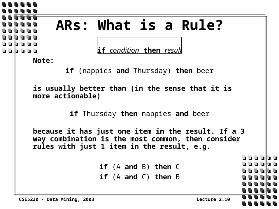
ARs: What is a Rule?
if condition then result
Note:
if (nappies and Thursday) then beer
is usually better than (in the sense that it is more actionable)
if Thursday then nappies and beer
because it has just one item in the result. If a 3 way combination is the most common, then consider rules with just 1 item in the result, e.g.
if (A and B) then C
if (A and C) then B

CSE5230 - Data Mining, 2003 Lecture 2.11
AR: Is the Rule a Useful Predictor? (1)
Confidence is the ratio of the number of transactions with all the items in the rule to the number of transactions with just the items in the condition. Consider:
if B and C then A
If this rule has a confidence of 0.33, it means that when B and C occur in a transaction, there is a 33% chance that A also occurs.

CSE5230 - Data Mining, 2003 Lecture 2.12
AR: Is the Rule a Useful Predictor? (2)
Consider the following table of probabilities of items and their combinations:
Combination ProbabilityA 0.45B 0.42C 0.40A and B 0.25A and C 0.20B and C 0.15A and B and C 0.05

CSE5230 - Data Mining, 2003 Lecture 2.13
AR: Is the Rule a Useful Predictor? (3)
Now consider the following rules:
It is tempting to choose “If B and C then A”, because it is the most confident (33%) - but there is a problem
Rule p(condition) p(condition confidenceand result)
if A and B then C 0.25 0.05 0.20if A and C then B 0.20 0.05 0.25if B and C then A 0.15 0.05 0.33

CSE5230 - Data Mining, 2003 Lecture 2.14
This rule is actually worse than just saying that A randomly occurs in the transaction - which happens 45% of the time
A measure called improvement indicates whether the rule predicts the result better than just assuming the result in the first place
p(condition and result)
p(condition)p(result)
AR: Is the Rule a Useful Predictor? (4)
improvement =
CSE5230 - Data Mining, 2003 Lecture 2.15
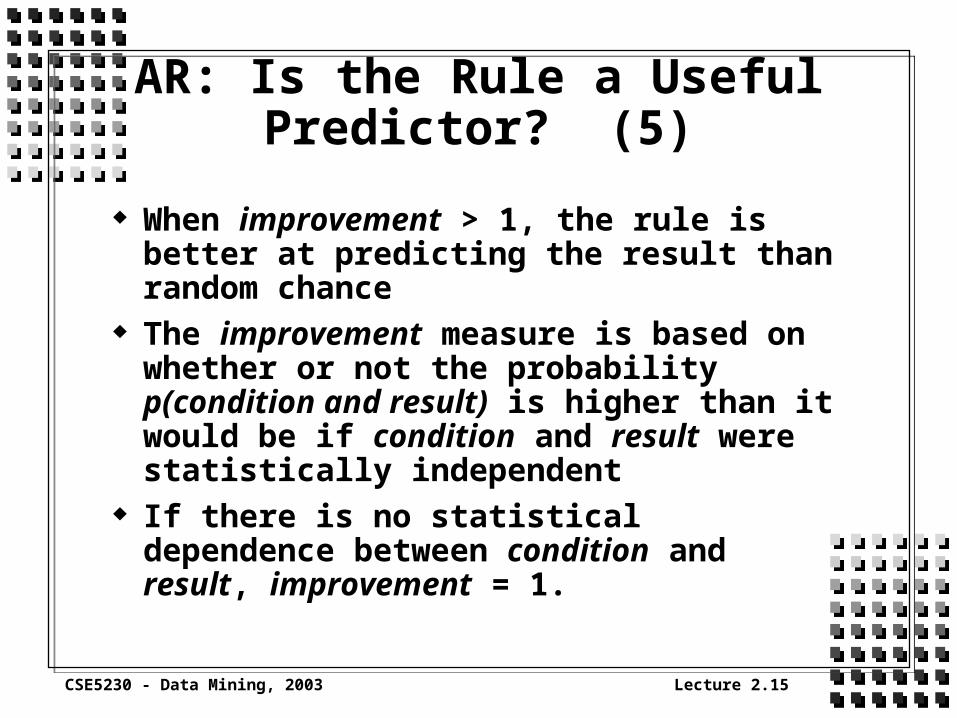
AR: Is the Rule a Useful Predictor? (5)
When improvement > 1, the rule is better at predicting the result than random chance
The improvement measure is based on whether or not the probabilityp(condition and result) is higher than it would be if condition and result were statistically independent
If there is no statistical dependence between condition and result, improvement = 1.

CSE5230 - Data Mining, 2003 Lecture 2.16
AR: Is the Rule a Useful Predictor? (6)
Consider the improvement for our rules:
Rule support confidence improvement
if A and B then C 0.05 0.20 0.50
if A and C then B 0.05 0.25 0.59
if B and C then A 0.05 0.33 0.74
if A then B 0.25 0.59 1.31
None of the rules with three items shows any improvement - the best rule in the data actually has only two items: “if A then B”. A predicts the occurrence of B 1.31 times better than chance.

CSE5230 - Data Mining, 2003 Lecture 2.17
AR: Is the Rule a Useful Predictor? (7)
When improvement < 1, negating the result produces a better rule. For example
if B and C then not A
has a confidence of 0.67 and thus an improvement of 0.67/0.55 = 1.22
Negated rules may not be as useful as the original association rules when it comes to acting on the results

CSE5230 - Data Mining, 2003 Lecture 2.18
AR: Discovering Large Item Sets
The term “frequent itemset” means “a set S that appears in at least fraction s of the baskets,” where s is some chosen constant, typically 0.01 (i.e. 1%).
DM datasets are usually too large to fit in main memory. When evaluating the running time of AR discovery algorithms we:
count the number of passes through the data
» Since the principal cost is often the time it takes to read data from disk, the number of times we need to read each datum is often the best measure of running time of the algorithm.

CSE5230 - Data Mining, 2003 Lecture 2.19
AR: Discovering Large Item Sets (2)
There is a key principle, called monotonicity or the a-priori trick that helps us find frequent itemsets:
If a set of items S is frequent (i.e., appears in at least fraction s of the baskets), then every subset of S is also frequent.
To find frequent itemsets, we can:1. Proceed level-wise, finding first the frequent items (sets of
size 1), then the frequent pairs, the frequent triples, etc. Level-wise algorithms use one pass per level.
2. Find all maximal frequent itemsets (i.e., sets S such that no proper superset of S is frequent) in one (or few) passes
CSE5230 - Data Mining, 2003 Lecture 2.20
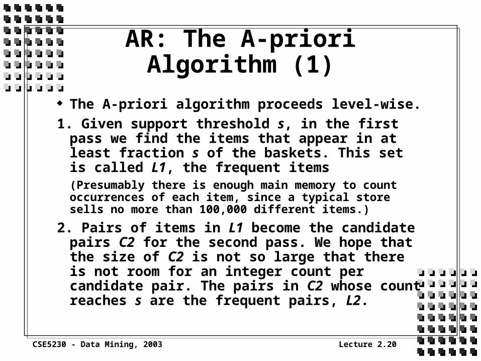
AR: The A-priori Algorithm (1)
The A-priori algorithm proceeds level-wise.
1. Given support threshold s, in the first pass we find the items that appear in at least fraction s of the baskets. This set is called L1, the frequent items
(Presumably there is enough main memory to count occurrences of each item, since a typical store sells no more than 100,000 different items.)
2. Pairs of items in L1 become the candidate pairs C2 for the second pass. We hope that the size of C2 is not so large that there is not room for an integer count per candidate pair. The pairs in C2 whose count reaches s are the frequent pairs, L2.

CSE5230 - Data Mining, 2003 Lecture 2.21
AR: The A-priori Algorithm (2)
3. The candidate triples, C3 are those sets {A, B, C} such that all of {A, B}, {A, C} and {B, C} are in L2. On the third pass, count the occurrences of triples in C3; those with a count of at least s are the frequent triples, L3.
4. Proceed as far as you like (or until the sets become empty). Li is the frequent sets of size i; Ci+1 is the set of sets of size i + 1 such that each subset of size i is in Li.
The A-priori algorithm helps because the number tuples which must be considered at each level is much smaller than it otherwise would be.
CSE5230 - Data Mining, 2003 Lecture 2.22
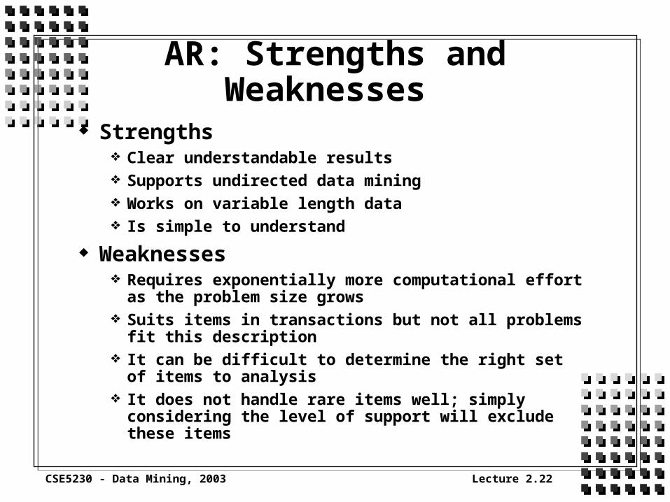
AR: Strengths and Weaknesses
Strengths Clear understandable results Supports undirected data mining Works on variable length data Is simple to understand
Weaknesses Requires exponentially more computational effort as the
problem size grows Suits items in transactions but not all problems fit this
description It can be difficult to determine the right set of items to
analysis It does not handle rare items well; simply considering the
level of support will exclude these items

CSE5230 - Data Mining, 2003 Lecture 2.23
Machine Learning
“A general law can never be verified by a finite number of observations. It can, however, be falsified by only one observation.”
Karl Popper
The patterns that machine learning algorithms find can never be definitive theories
Any results discovered must to be tested for statistical relevance

CSE5230 - Data Mining, 2003 Lecture 2.24
The Empirical Cycle
Analysis
Observation Theory
Prediction

CSE5230 - Data Mining, 2003 Lecture 2.25
Concept Learning (1)
Example: the concept of a wombat a learning algorithm could consider the characteristics
(features) of many animals and be advised in each case whether it is a wombat or not. From this a definition would be deduced.
The definition is complete if it recognizes all instances of a concept ( in
this case a wombat). consistent if it does not classify any negative examples
as falling under the concept.

CSE5230 - Data Mining, 2003 Lecture 2.26
Concept Learning (2)
An incomplete definition is too narrow and would not recognize some wombats.
An inconsistent definition is too broad and would classify some non-wombats as wombats.
A bad definition could be both inconsistent and incomplete.

CSE5230 - Data Mining, 2003 Lecture 2.27
Hypothesis Characteristics
Classification Accuracy 1 in a million wrong is better than 1 in 10 wrong.
Transparency A person is able understand the hypothesis generated. It is then
much easier to take action
Statistical Significance The hypothesis must perform better than the naïve prediction.
Imagine a situation where 80% of all animals considered are wombats. A theory that all animals are wombats would be is right 80% of the time! But nothing would have been learnt about classifying animals on the basis of their characteristics.
Information Content We look for a rich hypothesis. The more information contained
(while still being transparent) the more understanding is gained and the easier it is to formulate an action plan.

CSE5230 - Data Mining, 2003 Lecture 2.28
Complexity of Search Space
Machine learning can be considered as a search problem. We wish to find the correct hypothesis from among many.
If there are only a few hypotheses we could try them all but if there are an infinite number we need a better strategy.
If we have a measure of the quality of the hypothesis we can use that measure to select potential good hypotheses and based on the selection try to improve the theories (hill-climbing search)
Consider the metaphor of the kangaroo in the mist (see example on whiteboard).
This demonstrates that it is important to know the complexity of the search space. Also that some pattern recognition problems are almost impossible to solve.

CSE5230 - Data Mining, 2003 Lecture 2.29
Learning as a Compression
We have learnt something if we have an algorithm that creates a description of the data that is shorter than the original data set
A knowledge representation is required that is incrementally compressible and an algorithm that can achieve that incremental compression
The file-in could be a relation table and the file-out a prediction or a suggested clustering
AlgorithmFile-in File-out
CSE5230 - Data Mining, 2003 Lecture 2.30
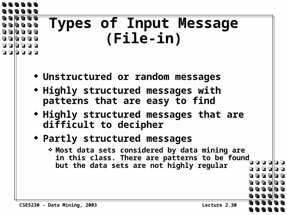
Types of Input Message (File-in)
Unstructured or random messages Highly structured messages with patterns
that are easy to find Highly structured messages that are difficult
to decipher Partly structured messages
Most data sets considered by data mining are in this class. There are patterns to be found but the data sets are not highly regular

CSE5230 - Data Mining, 2003 Lecture 2.31
Minimum Message Length Principle The best theory to explain data set is the one
that minimizes the sum of the length, in bits, of the description of the theory, plus the length of the data when encoded using the theory.
01100011001001101100011010101111100100110
00110011000011 110001100110000111
i.e., if regularity is found in a data set and the description of this regularity together with the description of the exceptions is still shorter than the original data set, then we have found something of value.
CSE5230 - Data Mining, 2003 Lecture 2.32
Noise and Redundancy
The distortion or mutation of a message is the number of bits that are corrupted
making the message longer by including redundant information can ensure that a message is received correctly even in the presence of noise
Some pattern recognition algorithms cope well with the presence of noise, others do not
We could consider a database which lacks integrity to contain a large amount of noise
patterns may exist for a small percentage of the data due solely to noise

CSE5230 - Data Mining, 2003 Lecture 2.33
References
Berry J.A. & Linoff G.; Data Mining Techniques: For Marketing, Sales, and Customer Support ; John Wiley & Sons, Inc.; 1997
Rakesh Agrawal and Ramakrishnan Srikant, Fast Algorithms for Mining Association Rules, In Jorge B. Bocca, Matthias Jarke and Carlo Zaniolo eds., VLDB'94, Proceedings of the 20th International Conference on Very Large Data Bases, Santiago de Chile, Chile, pp. 487-499, September 12-15 1994
CSE5230 web site links page