CSE3180 Summer 2005. Lect 4 / 1 Lecture No. 4. CSE3180 Summer 2005. Lect 4 / 2 Lecture 4 Structured...

CSE3180 Summer 2005. Lect 4 / 1

Lecture No. 4Lecture No. 4


Lecture 4Lecture 4

Structured Query Language - SQLCommandsStatements

QueriesViews


PowerPoint OverheadsPowerPoint OverheadsPowerPoint OverheadsPowerPoint Overheads

• The Overheads and other materials are accessible via

http://www.csse.monash.edu.au/courseware/cse3180s

• Files should be saved and copied to A:\ or D:\ (filename)

• Then you can browse these via PowerPoint97/2000

• or you can display them on the terminal screen (in the labs this will be Office 2000 software).


Doctor’s DiaryDoctor’s Diary

1. I examined your patient today who is still under our car for physical therapy

2. Discharge status : Alive, but without my permission


ObjectivesObjectives

• This lecture we will be looking at some of the aspects and functions of SQL - Structured Query Language, which provides the means of accessing data in a Relational Data Base.

• Microsoft Access provides users with a Graphics User Interface which in turn is translated into (non standard) SQL

• When you have developed part of your assignment in Access, run a query, and then display the query in its SQL statement form. You should be easily able to recognise the table names and the functions you have set up.


Objectives - cont’dObjectives - cont’dObjectives - cont’dObjectives - cont’d

The objectives of this lecture are

1. To introduce the Data Definition and Data Manipulation components of SQL (Structured Query Language) as expressed in Oracle

2. To proceed through some of the SQL commands such as Select, From, Where, Having, Group By, Order By

3. To introduce other components such as Logical Operators, Arithmetic Operators, Sub-queries and Views


ObjectivesObjectives

As we work through the material and the examples, I will point out the functions or facilities which Access provides, and there will be some SQLServer2000 references.

Summer Semester 2000. Lect 4 / 8

SQL - Data ManipulationSQL - Data Manipulation

SQL Structured Query Language

Originally designed and implemented by IBM research as the interface to a relational database.

ANSI Standard 1986. SQL99 Standard released. (SQL3)

A declarative language.

The DBMS performs retrieval.

A choice of access routines is made to optimise the query.

SQL specifies syntax features for definition of the database tables, retrieval, and update


Firstly some plusses for SQL.

1. SQL is the one industry standard for querying databases

2. Other ‘tools’ such as front enders don’t allow the developer to use all of the features of a database

3. Tools provided invariably do not exploit the full functionality of the underlying language

4. An SQL query in a client-server environment can be run in any application language and the result will always be the same

An Introduction to SQLAn Introduction to SQL


SQL requires a different approach from that used in other programming languages

C, Fortran, Basic, Cobol, Pascal, PL/1 are procedural languages. They are characterised by statements which tell the executing computer what to do, and in a structured step-by-step way (even when loops are used).

SQL is a declarative language - the computer is told what the user wants to achieve and the computer ‘decides’ on how to achieve this requirement, and correctly.

The user sees the results.

Procedural and Non-Procedural LanguagesProcedural and Non-Procedural Languages


SQL acts as a bridge between

– the user

– the database management system (DBMS)

– the data tables

– the transactions which involve the previous 3 items

SQL also allows the ‘system’ to be administered and

managed by a database administrator using the same

format : procedural commands and data in tables.

SQL can be embedded into source code (C, Cobol, C+

+, Java)

Some SQL Basics Some SQL Basics


SQL Some VariationsSQL Some Variations

• Microsoft Access SQL is mostly ANSI-89 Level 1 compliant. (watch SQLServer as a replacement)

• Some ANSI SQL features are not implemented in Access SQL

• MS Access SQL includes reserved words and features not supported in ANSI SQL

• Some differences– Matching character MS Access ANSI SQL

Single character ? _

Zero or more chars * %• MS Access does not support COMMIT, GRANT, LOCK• DISTINCT aggregate functions (eg SUM(DISTINCT att)


Some Aspects of SQLSome Aspects of SQL

The language consists of commands which allow users (with appropriate privileges) to– create database and table structures– perform data manipulations– perform database administration– query a database to extract information

All relational Database Management Systems support SQL

Many software vendors have developed extensions to the basic SQL command set



SQL is a non-procedural language

The user specifies what is to be done, but not how (which invariably irritates and confuses ‘normal’ software language developers

Complex activities required to perform a process are the function of SQL, not detailed user code software

Some of the advanced features of SQL include– stored procedures and triggers– conditions and looping



It is not meant to ‘stand alone’ in the applications area

It is not intended to create menus, special report forms, overlays, pop-ups,..

These features are normally supplied as vendor-enhancements

It is a data management and extraction tool


SQL and its ANSI SupportSQL and its ANSI Support

• There is a National Committee for Information Technology Standards - NCITS.

• There is a H2 Technical Committee which reports to NCITS on matters of database - and in particular database processing capabilities. This was previously ANSI X3H2

• Successful recommendations are then proposed to and invariably accepted by the American National Standards Institute

• Another ‘working group’ is the Object Management Group (OMJ) which also has a Technical Committee

• These 2 Committees are responsible for the framework for co-operation between SQL and Java, and SQL and XML


DDL - Data DefinitionDDL - Data Definition

CREATE (1) TABLE - define table name, attributes, types

(2) VIEW - define user view of data

(3) INDEX - create index on nominated attributes

DROP (1) TABLE - delete table, attributes and values

(2) VIEW - delete user view(s)

(3) INDEX - delete index, indexes

NOTE: Ingres and Oracle support the 'owner' concept.

Hence only 'owners' can DROP nnnn

Oracle 8i has an ALTER command to vary attribute characteristics. Ingres V6.4 does not support this feature


DML - Data Manipulation LanguageDML - Data Manipulation Language

Group 1 - Data Modification

INSERT - Add a single row (interactive)

- Perform successive INSERTS as a 'transaction ‘set’ - interactive

COPY - From an external file to a database table

- From a table to an external file

UPDATE - Amend attribute values in rows

DELETE - Delete rows of data from a table

WHEN IN DOUBT, USE HELP or DOCUMENTATION.


DML - Data Manipulation LanguageDML - Data Manipulation LanguageGroup 2

DATA CONTROL - User control of transaction processing

COMMIT - Commit or enable changes to the database

ROLLBACK - Rollback and reprocess (or some other action) transaction which could not be COMMITTed .

Group 3

DATA SECURITY - Authority over users - generally only available to the DBA

GRANT - Allow access privileges to users (e.g. read,write,update to nominated tables or attribute values in tables)

REVOKE - Revoke or cancel access privileges


CREATECREATE

The Oracle based SQL syntax is :

create table <tablename> ( columnname format

{,columnname format})

e.g. create table wages(name varchar2(10),

identity number(2,0),

Department varchar2(3),

date_comm date);

The same table but with more constraints :-

create table wages(name varchar2(10) not null,

identity number(2,0) not null,

Department varchar2(3) not null,

date_comm date) not null;


Optional CREATEOptional CREATE

create table highincome

as select name, salary

from wages where salary > 75000; (attribute properties are copied to the new

table)

This creates an ‘extract file’ of only those entries from the table ‘wages’ where the salary is in excess of 75,000 (what currency ?)

It is NOT automatically updated unless there is either

(a) cascade update set with the referential integrity constraint

or (b) a trigger and constraint is developed for the 2 tables


INSERTINSERT

This command allows data to be inserted, one row at a time, into an existing table

Syntax: Insert into <tablename> (list of attributes)

values (list of values)

Note: The list of attributes can be ignored providing the order of attribute values, and completeness of attribute instances, is as per the table list.

example: insert into emp(name, sal, byear)

values(‘Jones, Bill’, 45000,1967);

or(see note) insert into emp values(‘Jones, Bill’, 45000,1968);


INSERT - an extensionINSERT - an extension

The Insert command can also use a feature similar to create, i.e. use data from an existing table to populate another table.

insert into job(jid, jtitle, lowsal, highsal)

select job_no, title, lowsal, highsal)

from newjob

where title = ‘system analyst’);

The attributes of the table ‘newjob’ comprise at least job_no,title, lowsal, highsal


Oracle - SQLLOADOracle - SQLLOAD

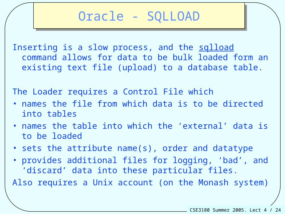
Inserting is a slow process, and the sqlload command allows for data to be bulk loaded form an existing text file (upload) to a database table.

The Loader requires a Control File which• names the file from which data is to be directed into tables• names the table into which the ‘external’ data is to be

loaded• sets the attribute name(s), order and datatype• provides additional files for logging, ‘bad’, and ‘discard’

data into these particular files.

Also requires a Unix account (on the Monash system)


Oracle LoaderOracle Loader

Some features :

skip - starting point of load

load - default of all

log - log of records

bad - log of discards

Control file : details of loader file, name of Oracle table to load into, column and field specifications


Import and ExportImport and Export

• These commands are available to the DBA and the application developers

• The commands make quick and dependable copies of Oracle data

• EXPORT makes a copy of data and data structures in a operating system file (external directory e.g. Unix)

• IMPORT reads file created by Export and places data and data structures into Oracle database tables

• Their uses are:– backup and recovery– moving data between instances of Oracle– moving data between tablespaces


CopyCopy

There are a number of forms associated with ‘COPY’

1. Copying data from 1 database to another

remote to local

local to remote

remote to remote

2.Copy data from one table to another (single database)

Copy data to one table from another

a sample:

copy from rsimpson@cse2180 (to the current database)

create empcopy2

using select * from user.dept


Access ImportAccess Import

• MS-Access offers an Import function which directs data from others sources (e.g. other Access databases, Excel, and various other sources such as SQL server) to an Access database. These sources can be local or remote.

• This serves the same purpose which is to use (or reuse) existing data and bulk copy to a target.

• Error messages (mismatches, data missing, data type mismatch etc) are generated as a by product of the process.

• The target database table (or tables) must be compatible with the source ( or is that vice - versa ?)


Database QueriesDatabase Queries

The commands which you have just seen are not normally available to ‘users’ as in Administration staff, Analytical staff, Review and Audit staff members.

They are invariably restricted to Designers, Software Application and Database Administration members.

The most frequent use of a database is associated with querying and retrieving data - and in many organisations these activities are embedded in host programs with menu options for individual user interaction - and here also there are privileges or restrictions on who can do what.


General Form of a QueryGeneral Form of a Query

SELECT as a function applies algebra in developing a result table from a base table, (or tables). The result table may have 0 to n rows...

The SELECT COMMAND is used to query data in the database..

Its syntax is : SELECT (select-list - attributes or derived data

FROM (table name or names)

WHERE (sets up conditions)

GROUP BY (attribute names)

HAVING (search-conditions)

ORDER BY (attribute name or names)


General Form of a QueryGeneral Form of a Query

SELECT and FROM are compulsory.

Other clauses are optional but occur in the order shown

HAVING is normally associated with GROUP BY


Select ExamplesSelect Examples

SELECT * FROM PART;

Selects all column values for all rows

SELECT PARTID, PNAME FROM PART

WHERE PRICE BETWEEN 0.2 AND 1.0;

Selects rows where price >= .2 and <= 1.0

SELECT PARTID, PNAME FROM PART

WHERE PNAME IN ('NUT','BOLT');

Selects rows where pname has a value in the following list

PARTPartID Pname Price QOHP1 Nut 0.2 20P2 Bolt 1 40P3 Caravan 5000 3


SELECTSELECT

SELECT pname, price*qoh AS Pvalue

FROM PART

WHERE price > 0.20 AND price * qoh > 30.0

ORDER BY pname desc;

Result Table --->

PARTPartID Pname Price QOHP1 Nut 0.2 20P2 Bolt 1 40P3 Caravan 5000 3

Pname PvalueCaravan 15000Bolt 40


Format of a Query ScriptFormat of a Query Script

SELECT (attribute list )

FROM (tables list)

WHERE (conditions for joins)

GROUP BY (selected groupings

HAVING (condition for grouping)

ORDER BY (Attribute(s) order [ Asc or Desc]


Expressions in SelectExpressions in Select

Arithmetic operators are + - ** * /

Comparison operators are = != <> ^= > < >= <=

Logical operators are AND OR NOT

Parentheses may be used to alter order of evaluation - unary, **, * /, + -

Wildcard % = any string of zero or more character

_ = any one character

[ ] = any of the characters enclosed in brackets

A range of numeric, string, date and other functions are available.


SELECT VocabularySELECT Vocabulary

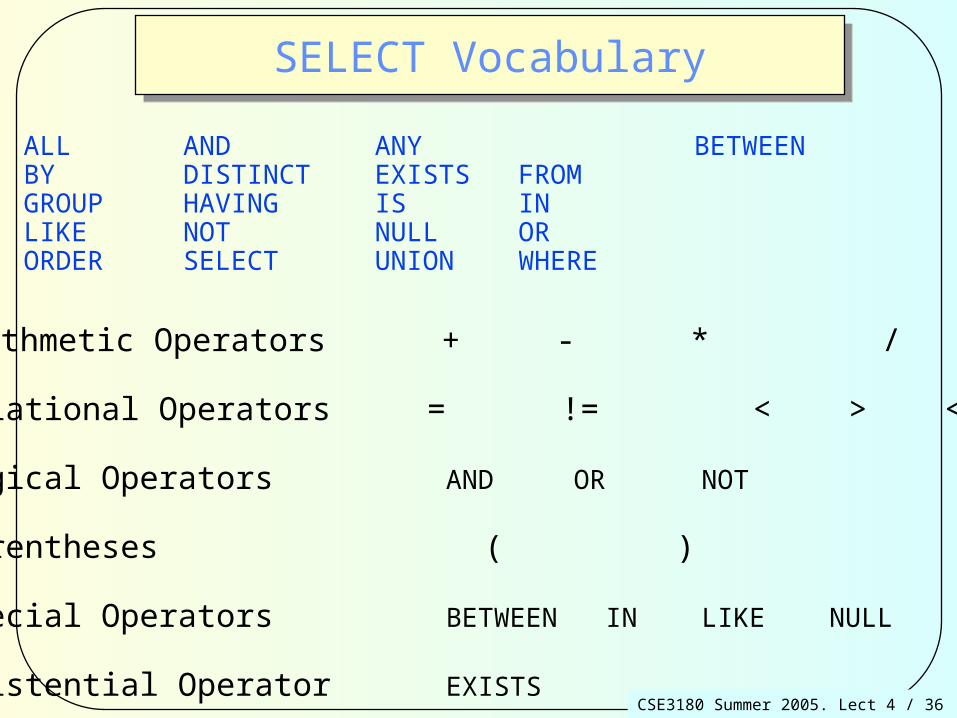
ALL AND ANY BETWEENBY DISTINCT EXISTS FROMGROUP HAVING IS INLIKE NOT NULL ORORDER SELECT UNION WHERE

Arithmetic Operators + - * /

Relational Operators = != < > <= >=

Logical Operators AND OR NOT

Parentheses ( )

Special Operators BETWEEN IN LIKE NULL

Existential Operator EXISTS


SQL - Sample Database SchemaSQL - Sample Database Schema

MARRIAGE

PM_NAME SPOUSE_NAME MAR_YR PM_AGE NR_CHILDREN

MINISTRY

MIN_NR PM_NAME PARTY DAY_COMM MTH_COMM YR_COMM

PM_NAME BIRTH_YR YRS_SERVED DEATH_AGE STATE_BORN STATE_REP

PRIME _MINISTER


Arithmetic OperatorsArithmetic Operators

List the name, birth year and year of death of each prime minister who was born in New South Wales. List in order of birth year.

SELECT PM_NAME, BIRTH_YR, BIRTH_YR + DEATH_AGEFROM PRIME_MINISTERWHERE STATE_BORN = ‘NSW’ORDER BY BIRTH_YR;

PM_NAME BIRTH_YR BIRTH_YR + DEATH_AGEBarton E 1849 1920Page E C G 1880 1961Chifley J 1885 1951Holt H E 1908 1967McMahon W 1908 ?Whitlam E G 1916 ?


Logical OperatorsLogical Operators

Which prime ministers were born in Victoria before the turn of the century?

SELECT PM_NAME, BIRTH_YR, STATE_BORNFROM PRIME_MINISTERWHERE STATE_BORN=‘VIC’ AND BIRTH_YR < 1900;

PM_NAME BIRTH_YR STATE_BORNDeakin A 1856 VICBruce S M 1883 VICScullin J H 1876 VICMenzies R G 1894 VICCurtin J 1885 VIC


Combining Logical OperatorsCombining Logical Operators

Which prime ministers were born in NSW and then represented Victoriaor have simply not served less than two years?

SELECT PM_NAME, STATE_BORN, STATE_REP, YRS_SERVEDFROM PRIME _MINISTERWHERE STATE_REP = ‘VIC’AND STATE_BORN = ‘NSW’OR NOT YRS_SERVED < 2; (or Yrs_Served >1.99)PM_NAME STATE_BORN STATE_REP YRS_SERVEDHolt H E NSW VIC 1.88Gorton J G VIC VIC 3.17Whitlam E G NSW NSW 2.92Fraser J M VIC VIC 7.33


Select Examples - ‘PART’ tableSelect Examples - ‘PART’ table

SELECT PNAME FROM PART

WHERE QOH IS NULL;

Selects those rows where qoh has a null value (is this different from a 0 value ?)

SELECT * FROM PART

WHERE PNAME LIKE '_ _T' or PNAME LIKE '%LT';

Selects rows where pname has three letters the last of which is a T or PNAME ends in LT

And the answer to the question above is ‘Definitely YES’


Use of COUNT and Distinct operatorsUse of COUNT and Distinct operators

How many Liberal prime ministers were commissioned between 1970 and 1980?

SELECT ‘Liberal PMs’, COUNT(*), COUNT(DISTINCT PM_NAME)FROM MINISTRYWHERE PARTY = ‘Liberal’AND YR_COMM BETWEEN 1970 AND 1980;

COUNT(*) COUNT(DISTINCT PM_NAME)

Liberal PMs 5 2


UNION OperatorUNION Operator

Normally used with the SELECT command to form a single table from two or more tables. This can be a real or virtual table.

The attributes used in a UNION must be identical - in data type and size.

example: create table names as select name from master

union select newnames from newmaster;


UnionUnion

Assume that the following ‘Names’ data is contained in 2 tables

Longtime Prospect

Adah Talbot Adah Talbot

Dick Jones Dory Kenson

Donald Rollo Elbert Talbot

Elbert Talbot George Phepps

George Oscar Jed Hopkins

Pat Lavay Pat Lavay

Peter Lawson Ted Butcher

Wilfred Lowell Wilfred Lowell (8 names) (8 names)


UnionUnion

The statement select name from longtime

union

select name from prospect; would give this resultAdah Talbot

Dick Jones

Donald Rollo

Dory Kenson

Elbert Talbot

George Oscar

George Phepps note that there are NO duplicatesJed Hopkins

Pat Lavay

Peter Lawson

Ted Butcher

Wilfred Lowell

(12 names)


DELETEDELETE

DELETE FROM tablename [corr-name]

[ WHERE search-condition ]

Delete one or many rows in a table.

In general search-condition and qualification may not involve a sub select on tablename.

DELETE FROM PART WHERE qoh < 4.00;


UPDATEUPDATE

UPDATE tablename [corr-name]

[ FROM tablename [corr-name] {, tablename [corr-name]}]

SET colname = expression { , colname = expression}

[ WHERE search_condition ]Replaces values of the specified columns with expression values for all

rows satisfying the search condition.

Expressions in the set clause may be constants or column values from the UPDATE tablename or FROM tablename

UPDATE PART

SET price = price * 1.1

WHERE price < 20;


SET FunctionsSET Functions

• A SET Function is one which operates on an entire column of values, not just a single value

• The SET functions supported are:

Name Format(Result) Description

count integer Count of Occurrences

sum integer,float,money Summation

avg float,money Average (sum/count)

max same as the argument Maximum value

min same as the argument Minimum value


Use of SET functionsUse of SET functions

Set functions supported: avg count max min sum

Set functions may not be used directly in a search condition

SELECT count(PartID) AS Part_count, avg(price) AS Av_price, count(distinct price) AS Price_count FROM part;

PARTPartID Pname Price QOHP1 Nut 1.00 20P2 Bolt 1.00 20P3 Caravan 5000 3

Part_count Av_price Price_count 3 1667.33 2


Use of GROUP BYUse of GROUP BY

List the number of prime ministers from each party.

SELECT PARTY, COUNT(*)FROM MINISTRYGROUP BY PARTY;

PARTY COUNT(*)Country 3Free Trade 1Labor 15Liberal 17National Labor 1Nationalist 3Protectionist 4United Australia 5


Grouping by More than One AttributeGrouping by More than One Attribute

Group prime ministers by their state born and by the state they represented.Give the numbers of prime ministers and the total numbers of years served.

SELECT STATE_BORN, STATE_REP, COUNT(*), SUM(YRS_SERVED)FROM PRIME_MINISTERGROUP BY STATE_BORN, STATE_REP;

STATE_BORN STATE_REP COUNT(*) SUM(YRS_SERVED)? NSW 4 9.67? QLD 1 4.81NSW NSW 5 11.83NSW VIC 1 1.88QLD QLD 2 0.13TAS TAS 1 7.25VIC VIC 7 42.69VIC WA 1 3.75


Grouping with the WHERE ClauseGrouping with the WHERE Clause

For prime ministers born after 1900, list the number of prime ministersborn in each state and the total number of years served.

STATE_BORN COUNT(*) SUM(YRS_SERVED)WA 1 ?VIC 2 10.50NSW 3 6.52

SELECT STATE_BORN, COUNT(*), SUM(YRS_SERVED)FROM PRIME_MINISTERWHERE BIRTH_YR > 1900GROUP BY STATE_BORN;


Grouping with the HAVING ClauseGrouping with the HAVING Clause

For each state where the total years served by prime ministers born in thatstate is less than 10 years, give the number of prime ministersborn in that state and the total number of years served.

SELECT STATE_BORN, COUNT(*), SUM(YRS_SERVED)FROM PRIME_MINISTERGROUP BY STATE_BORNHAVING SUM(YRS_SERVED) < 10;

STATE_BORN COUNT(*) SUM(YRS_SERVED)TAS 1 7.25QLD 2 0.13


Grouping with the HAVING ClauseGrouping with the HAVING Clause

SELECT PartID, Count(SuppID) AS Supp_count, Sum(qty_supp) Total_qty

FROM part_supplier

GROUP BY PartID

HAVING count(SuppID) > 1;

PART_SUPPLIER

PartID SuppID Qty_SuppP1 S1 20P2 S1 30P1 S2 20P3 S2 10

PartID Supp_count Qty_SuppP1 2 40


SubQueriesSubQueries

Provide the facility of a query supplying dynamic values to another query for use in the search conditions of the mainquery.Example: Give the name and age at which death occurred for each Prime Minister who died at an age less than the average . List in order of age at death.

SELECT PM_NAME, DEATH_AGEFROM PRIME_MINISTERWHERE DEATH_AGE < ( SELECT AVG(DEATH_AGE) FROM PRIME_MINISTER);The subquery computes the average age at death.The main query then selects the appropriate names andages based on the values supplied by the sub-query.(in this case where the age at death is less than the average)



Give the name and death age for each prime minister who died at an age less than the average death age of all prime ministers.List in ascending order of death age.

SELECT PM_NAME, DEATH_AGEFROM PRIME_MINISTERWHERE DEATH_AGE < (SELECT AVG(DEATH_AGE) FROM PRIME_MINISTER);ORDER BY DEATH AGE

PM_NAME DEATH_AGEHolt H E 59Lyons J A 60Curtin J 60Deakin A 63



Which prime minister died the oldest? Give the name and that age.

SELECT PM_NAME, DEATH_AGEFROM PRIME_MINISTERWHERE DEATH_AGE = (SELECT MAX(DEATH_AGE) FROM PRIME_MINISTER);

PM_NAME DEATH_AGEForde F M 93


SubQuery with IN OperatorSubQuery with IN Operator

SELECT DISTINCT DEPUTY_NAME, PARTYFROM DEPUTY_PMWHERE DEPUTY_NAME IN (SELECT PM_NAME FROM PRIME_MINISTER);

DEPUTY_NAME PARTYChifley J B LaborCook J Free TradeCook Nationalist Deakin A Protectionist

List the name and party of each deputy prime minister who was also a Prime Minister.


SubQuery with ANY OperatorSubQuery with ANY Operator

PART_SUPPLIER

SELECT PartID, SuppID, qty_supp FROM Part_supplier

WHERE qty_supp > ANY

(SELECT avg(qty_supp) FROM Part-supplier);

PartID SuppID Qty_SuppP1 S1 20P2 S1 30P1 S2 20P3 S2 10

PartID SuppID Qty_SuppP2 S1 30P1 S2 25


Multiple Nested SubQueriesMultiple Nested SubQueries

Give the name and birth year of each prime minister who was commissioned after Bob Hawke had turned 21. Order by birth year.

SELECT PM_NAME, BIRTH_YRFROM PRIME_MINISTERWHERE PM_NAME = ANY (SELECT PM_NAME FROM MINISTRY WHERE YR_COMM > (SELECT BIRTH_YR + 21 FROM PRIME_MINISTER WHERE PM_NAME = ‘Hawke R J L’)) AND PM_NAME <> ‘Hawke R J L’ ORDER BY BIRTH_YR;


Result of Previous QueryResult of Previous Query

Give the name and birth year of each prime minister

who was commissioned after Bob Hawke had turned 21.

Order by birth year.

PM_NAME BIRTH_YR

Menzies R G 1894

McEwan J 1900

Holt H E 1908

McMahon W 1908

Gorton J G 1911

Whitlam E G 1916


A Search and Join ConditionA Search and Join Condition

For each prime minister born in or after 1900, give the name, birth year and party.

SELECT P.PM_NAME, BIRTH_YR, PARTYFROM PRIME_MINISTER P, MINISTRY MWHERE P.PM_NAME = M.PM_NAME AND BIRTH_YR >= 1900;

PM_NAME BIRTH_YR PARTYHolt H E 1908 LiberalHolt H E 1908 LiberalMcEwen J 1900 CountryGorton J G 1911 LiberalGorton J G 1911 LiberalGorton J G 1911 Liberal



SELECT PartID, SuppID, qty_supp FROM Part_supplier


(SELECT avg(qty_supp) FROM Part-supplier);

Subqueries may be used in a number of SQL statements.

select, update, insert, delete, create table,

create view, create permit, create integrity

· Subqueries may be nested to several levels.

· Special comparison operators are used in additional to =, <>, >, <, etc to indicate comparison to a set of values:

IN equals one of the values returned by the subquery

ANY true if any value returned meets the condition

ALL true if all values returned meet the condition


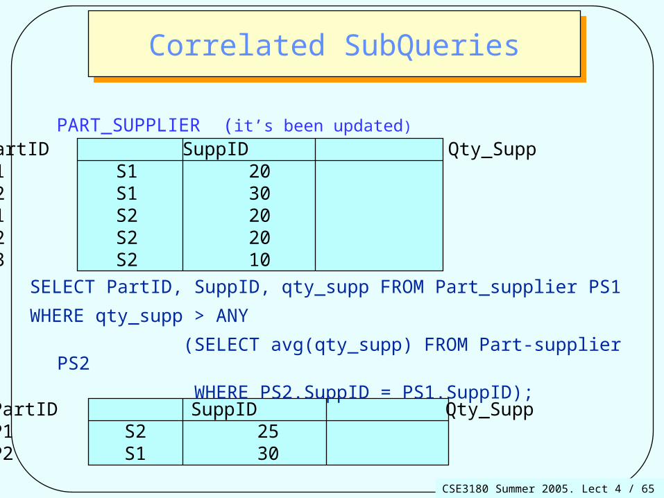
Correlated SubQueriesCorrelated SubQueries

PART_SUPPLIER (it’s been updated)

SELECT PartID, SuppID, qty_supp FROM Part_supplier PS1


(SELECT avg(qty_supp) FROM Part-supplier PS2

WHERE PS2.SuppID = PS1.SuppID);

PartID SuppID Qty_SuppP1 S1 20P2 S1 30P1 S2 20P2 S2 20P3 S2 10

PartID SuppID Qty_SuppP1 S2 25P2 S1 30


Correlated SubQueriesCorrelated SubQueries

SELECT PartID, SuppID, qty_supp

FROM Part_supplier PS1


(SELECT avg(qty_supp) FROM Part-supplier PS2

WHERE PS2.PartID = PS1.PartID);

· Subqueries (inner queries) are generally executed once and return a set of values to the outer query.

· With a correlated subquery, the outer query passes values to the inner query which then evaluates and returns a set of values to the outer query. This process repeats until the outer query terminates.

Which suppliers are supplying more than the average for a part and how much of that part do they supply?


Joining TablesJoining Tables

DEP

SELECT e.empid AS Number, e.ename AS Name, d.dname AS Department

FROM emp e, dep d

WHERE e.deptid = d.deptid;

DeptID DnameD1 TaxD2 PayD3 Leave

EMP

EmpID Ename MgrID DeptIDE1 Red E1 D1E2 Blue E1 D1E3 Brown E1 D2

Number Name DepartmentE1 Red TaxE2 Blue TaxE3 Brown Pay


A Search and Join ConditionA Search and Join Condition


SELECT P.PM_NAME, BIRTH_YR, PARTYFROM PRIME_MINISTER P, MINISTRY MWHERE P.PM_NAME = M.PM_NAME AND BIRTH_YR >= 1900;

PM_NAME BIRTH_YR PARTYHolt H E 1908 LiberalHolt H E 1908 LiberalMcEwen J 1900 CountryGorton J G 1911 LiberalGorton J G 1911 LiberalGorton J G 1911 Liberal


A Search and Join Condition


SELECT DISTINCT P.PM_NAME, BIRTH_YR, PARTYFROM PRIME_MINISTER P, MINISTRY MWHERE P.PM_NAME = M.PM_NAME AND BIRTH_YR >= 1900;

PM_NAME BIRTH_YR PARTYFraser J M 1930 LiberalGorton J G 1911 LiberalHawke R J L 1929 LaborHolt H E 1908 LiberalMcEwan J 1900 CountryMcMahon W 1908 LiberalWhitlam E G 1916 Labor

With ‘distinct’


Multiple JoinsMultiple Joins

SELECT DISTINCT P.PM_NAME, BIRTH_YR, MAR_YR, PARTYFROM PRIME_MINISTER P, PM_MARRIAGE W, MINISTRY MWHERE P.PM_NAME = W.PM_NAMEAND P.PM_NAME = M.PM_NAMEAND BIRTH_YR >= 1900;

PM_NAME BIRTH_YR MAR_YR PARTYFraser J M 1930 1956 LiberalGorton J G 1911 1935 LiberalHawke R J L 1929 1956 LaborHolt H E 1908 1946 Liberal

Give the name, birth year, party and the year of marriage of prime ministers born in or after 1900.


Anatomy of the Previous QueryAnatomy of the Previous Query

WHERE P.PM_NAME = W.PM_NAME

AND P.PM_NAME = M.PM_NAME

AND BIRTH_YEAR >= 1900 ;

SELECT DISTINCT P.PM_NAME, BIRTH_YR, MAR-YR, PARTY FROM PRIME_MINISTER P, PM_MARRIAGE W, MINISTRY M


Joining a Table to ItselfJoining a Table to Itself

SELECT X.empno AS Number, X.ename AS Name, Y.ename AS Manager

FROM emp X, emp Y

WHERE X.mgrno = Y.empno;

EMP

EmpID Ename MgrID DeptIDE1 Red E1 D1E2 Blue E1 D1E3 Brown E1 D2

Number Name ManagerE1 Red RedE2 Blue RedE3 Brown Red


The Existential OperatorThe Existential Operator

This is a test for Existence (or non-existence)

It differs from the IN operator in that it does not match a column or columns used in a correlated sub-query

A query such as this : select name from workerskill group by name having count (skill) > 1;

would give a list of workers who had more than 1 skill from a table named workerskill.


The Existential OperatorThe Existential Operator

However if we attempt to find both the Name and Skill, the query will fail as the count is on the Primary Key, in this example, skill.

There is only one Primary Key per row, and therefore the COUNT > 1 cannot exceed 1, and the query must fail.

In using the Existential operator, we use a subterfuge and that is to have the query think that the inspected table occurs twice. (by correlation).


The Existential Operator

How is this done ?Let’s look at this ‘solution’.

Select name, skill from workerskill wswhere exists (select * from workerskill

where ws.name = name group by name having count(skill) > 1);

as an exercise, you might like to try a solution with the subquery such as ‘where name IN…... and then use a similar construction to the above


The EXISTS OperatorThe EXISTS Operator

List the name, birth year and state represented of prime ministers who were also deputy prime ministers.

SELECT PM_NAME, BIRTH_YR, STATE_REPFROM PRIME_MINISTERWHERE EXISTS (SELECT * FROM DEPUTY_PM WHERE DEPUTY_NAME = PM_NAME);

PM_NAME BIRTH_YR STATE_REPDeakin A 1856 VICCook J 1860 NSWHughes W M 1862 NSW


The NOT EXISTS OperatorThe NOT EXISTS Operator

SELECT PM_NAME, BIRTH_YR, DEATH_AGEFROM PRIME_MINISTER PWHERE NOT EXISTS (SELECT * FROM PM_RECREATION WHERE PM_NAME = P.PM_NAME);

PM_NAME STATE_REP DEATH_AGEReid G H NSW 73Fisher A QLD 66Cook J NSW 87

Give the name, state represented and death age of each prime minister who has no recreational interests.


Create ViewCreate View

CREATE VIEW view-name [ (colname { , colname} ) ] AS subselect

[WITH CHECK OPTION]

. Creates a virtual table by storing the view definition in the catalog.

· Updates, inserts and deletes are not permitted if the subselect accesses more than one base table; the view was created from a non-updatable view; any columns in the view are derived. Additionally inserts are not allowed if the view contains a where clause with the check option or if any not null not default column of the base table is not part of the view.

· The with check option will not allow update of columns that are part of the view's where clause.

· Provide logical data independence when base table structure changes.

· Same data may be seen in different ways by different users.

· Users perception may be simplified and views provide automatic security.


Create ViewCreate View

Emp (empid, empname, salary_pa, deptid)

Dept (deptid, deptname)

CREATE VIEW empdetails (empid, empname, deptname, salary_fn) AS

SELECT e.empid, e.empname, d.deptname,

e.salary_pa / 26

FROM emp e, deptname d

WHERE e.deptid = d.deptid;


To Run a VIEWTo Run a VIEW

Select * from (View Name);

• Other conditions may be applied at runtime which to supplement those already contained in the View construct

e.g. Select * from empdetails

where deptname = ‘Finance’ ;

There is an ‘updatable view’ process which is possible, but with much constraint. There is a paper on this at the website.

CSE3180 Summer 2005. Lect 4 / 1 Lecture No. 4. CSE3180 Summer 2005. Lect 4 / 2 Lecture 4 Structured...

Documents

Transcript of CSE3180 Summer 2005. Lect 4 / 1 Lecture No. 4. CSE3180 Summer 2005. Lect 4 / 2 Lecture 4 Structured...