CSE182-L18

Population Genetics

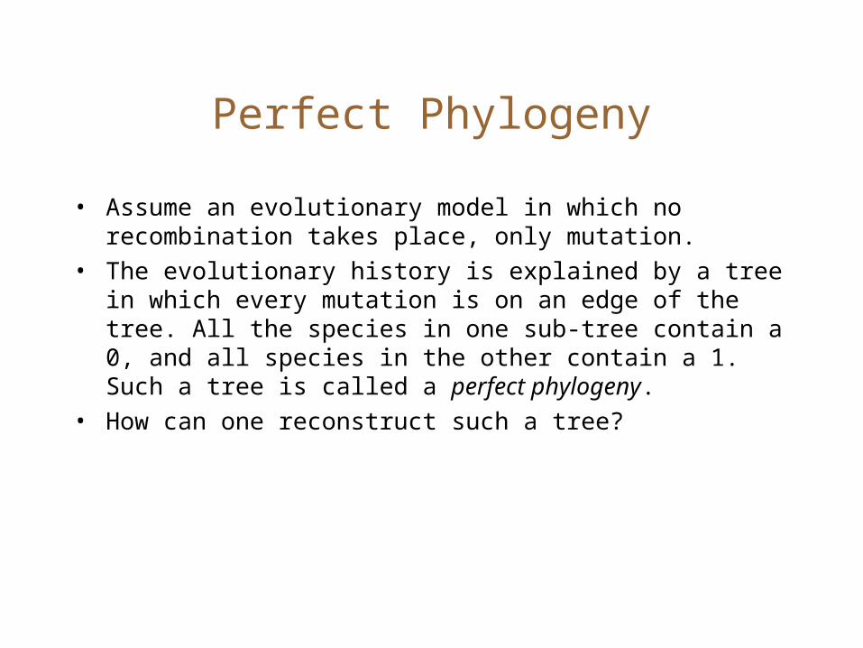
Perfect Phylogeny

• Assume an evolutionary model in which no recombination takes place, only mutation.

• The evolutionary history is explained by a tree in which every mutation is on an edge of the tree. All the species in one sub-tree contain a 0, and all species in the other contain a 1. Such a tree is called a perfect phylogeny.

• How can one reconstruct such a tree?

The 4-gamete condition

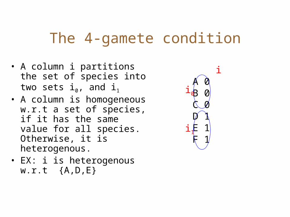
• A column i partitions the set of species into two sets i0, and i1

• A column is homogeneous w.r.t a set of species, if it has the same value for all species. Otherwise, it is heterogenous.

• EX: i is heterogenous w.r.t {A,D,E}

iA 0B 0C 0D 1E 1F 1

i0

i1

4 Gamete Condition

• 4 Gamete Condition– There exists a perfect phylogeny if and only if for all pair of

columns (i,j), either j is not heterogenous w.r.t i0, or i1.

– Equivalent to– There exists a perfect phylogeny if and only if for all pairs

of columns (i,j), the following 4 rows do not exist(0,0), (0,1), (1,0), (1,1)

4-gamete condition: proof

• Depending on which edge the mutation j occurs, either i0, or i1 should be homogenous.

• (only if) Every perfect phylogeny satisfies the 4-gamete condition

• (if) If the 4-gamete condition is satisfied, does a prefect phylogeny exist?

i0 i1

i

An algorithm for constructing a perfect phylogeny

• We will consider the case where 0 is the ancestral state, and 1 is the mutated state. This will be fixed later.

• In any tree, each node (except the root) has a single parent.– It is sufficient to construct a parent for every node.

• In each step, we add a column and refine some of the nodes containing multiple children.

• Stop if all columns have been considered.

Inclusion Property

• For any pair of columns i,j

– i < j if and only if i1 j1

• Note that if i<j then the edge containing i is an ancestor of the edge containing i

i

j

Example

1 2 3 4 5A 1 1 0 0 0B 0 0 1 0 0C 1 1 0 1 0D 0 0 1 0 1E 1 0 0 0 0

r

A B C D E

Initially, there is a single clade r, and each node has r as its parent

Sort columns

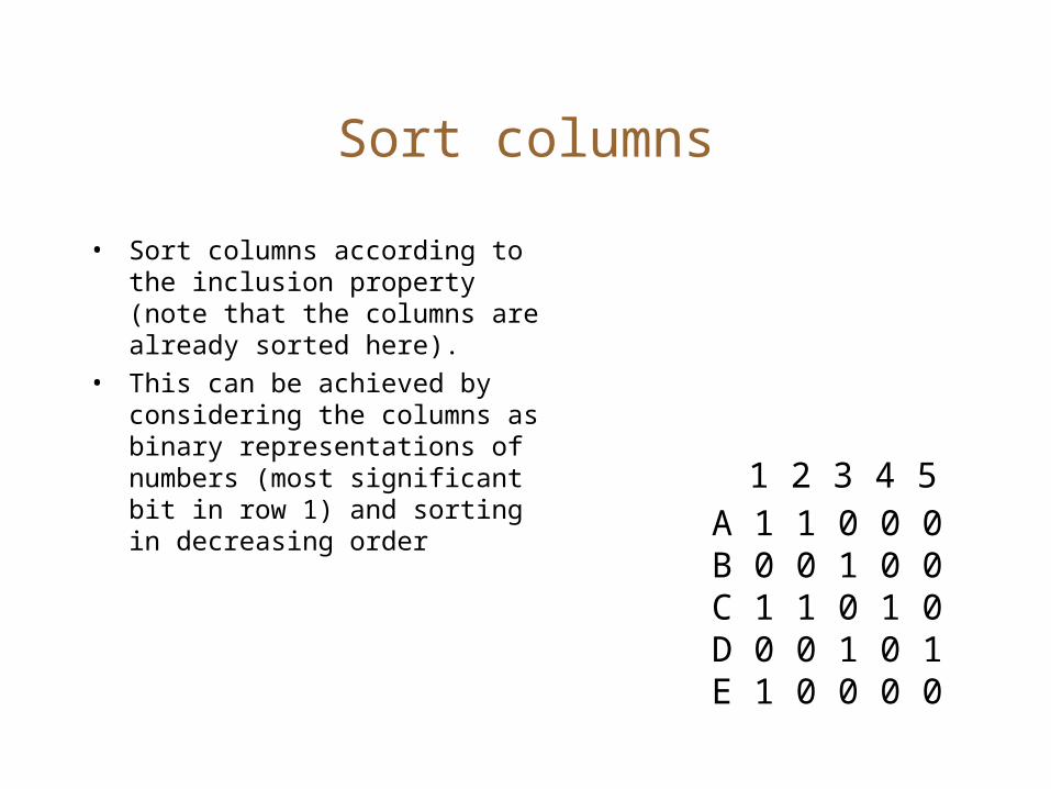
• Sort columns according to the inclusion property (note that the columns are already sorted here).

• This can be achieved by considering the columns as binary representations of numbers (most significant bit in row 1) and sorting in decreasing order

1 2 3 4 5A 1 1 0 0 0B 0 0 1 0 0C 1 1 0 1 0D 0 0 1 0 1E 1 0 0 0 0

Add first column

• In adding column i– Check each edge

and decide which side you belong.

– Finally add a node if you can resolve a clade

r

A BC DE

1 2 3 4 5

A 1 1 0 0 0B 0 0 1 0 0C 1 1 0 1 0D 0 0 1 0 1E 1 0 0 0 0

u

Adding other columns

• Add other columns on edges using the ordering property

r

E B

C

D

A

1 2 3 4 5

A 1 1 0 0 0B 0 0 1 0 0C 1 1 0 1 0D 0 0 1 0 1E 1 0 0 0 0

1

2

4

3

5

Unrooted case

• Switch the values in each column, so that 0 is the majority element.

• Apply the algorithm for the rooted case

Summary :No recombination leads to correlation between sites

0 0 0 0 0 0 0 0

0 0 1 0 0 0 0 0

0 0 1 0 0 0 0 1 0 0 1 0 1 0 0 0

3

8 5

• The different sites are linked. A 1 in position 8 implies 0 in position 5, and vice versa.

• The history of a population can be expressed as a tree.

• The tree can be constructed efficiently

A B

Recombination

• A tree is not sufficient as a sequence may have 2 parents

• Recombination leads to violation of 4 gamete property.

• Recombination leads to loss of correlation between columns

0000000011111111

00011111

Studying recombination

• A tree is not sufficient as a sequence may have 2 parents

• Recombination leads to loss of correlation between columns

• How can we measure recombination?

Linkage (Dis)-equilibrium (LD)

Extensive Recombination– Pr[A,B=(0,1)=0.125

• Linkage equilibrium

A B0 10 10 00 01 01 01 01 0

No recombination–Pr[A,B=0,1] = 0.25

•Linkage disequilibrium

A B0 00 10 00 01 11 01 01 0

Measuring LD

• Consider two bi-allelic sites A and B, with values 0 and 1.

• Let p1 = probability[individual has allele 1 in site A]

• q1 = probability[individual has allele 1 in site B]

• P11 = Prob [individual has allele 1 in site A, and B]

• Linkage Disequilibrium, D = |P11-p1q1| = |P01-p0q1| =….

• If D=0, sites are uncorrelated, (are in linkage equilibrium)

• If |D| >>0, sites are highly correlated (have high LD)• Other measures exist, but they all measure similar

quantities.

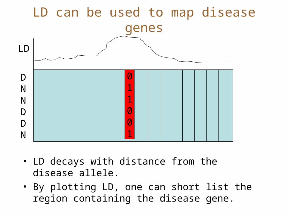
LD can be used to map disease genes

• LD decays with distance from the disease allele.

• By plotting LD, one can short list the region containing the disease gene.

011001

DNNDDN

LD

Population sub-structure can cause problems in disease gene

mapping

Population sub-structure can increase LD

• Consider two populations that were isolated and evolving independently.

• They might have different allele frequencies in some regions.

• Pick two regions that are far apart (LD is very low, close to 0)

0 .. 10 .. 10 .. 01 .. 10 .. 10 .. 10 .. 10 .. 10 .. 1

1 .. 01 .. 00 .. 01 .. 11 .. 01 .. 01 .. 01 .. 01 .. 0

Pop. A

Pop. B

p1=0.1q1=0.9P11=0.1D=0.01

p1=0.9q1=0.1P11=0.1D=0.01

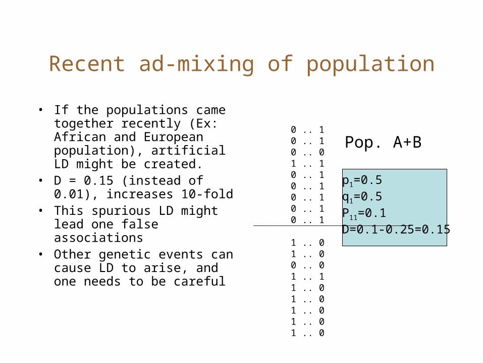
Recent ad-mixing of population

• If the populations came together recently (Ex: African and European population), artificial LD might be created.

• D = 0.15 (instead of 0.01), increases 10-fold

• This spurious LD might lead one false associations

• Other genetic events can cause LD to arise, and one needs to be careful

0 .. 10 .. 10 .. 01 .. 10 .. 10 .. 10 .. 10 .. 10 .. 1

1 .. 01 .. 00 .. 01 .. 11 .. 01 .. 01 .. 01 .. 01 .. 0

Pop. A+B

p1=0.5q1=0.5P11=0.1D=0.1-0.25=0.15

Determining population sub-structure

• Given a mix of people, can you sub-divide them into ethnic populations.

• Turn the ‘problem’ of spurious LD into a clue. – Find markers that are too far apart to show LD– If they do show LD (correlation), that shows the

existence of multiple populations.– Sub-divide them into populations so that LD

disappears.

Determining Population sub-structure

• Same example as before:• The two markers are too

similar to show any LD, yet they do show LD.

• However, if you split them so that all 0..1 are in one population and all 1..0 are in another, LD disappears

0 .. 10 .. 10 .. 01 .. 10 .. 10 .. 10 .. 10 .. 10 .. 1

1 .. 01 .. 00 .. 01 .. 11 .. 01 .. 01 .. 01 .. 01 .. 0

Iterative Algorithm for Population Substructure

• Assume that there are 2 sub-populations• Randomly partition the individuals into two.• Select an individual, and compute the

probabilities Pr(x|A), and Pr (x|B)• Assign the individual to A with probability

– Pr(x|A)/ (Pr(x|A)+Pr(x|B))

• Continue.

Iterative algorithm for population sub-structure

• Define• N = number of individuals (each has a single

chromosome)• k = number of sub-populations. • Z {1..k}N is a vector giving the sub-

population. – Zi=k’ => individual i is assigned to population k’

• Xi,j = allelic value for individual i in position j• Pk,j,l = frequency of allele l at position j in

population k

Example

• Ex: consider the following assignment

• P1,1,0 = 0.9

• P2,1,0 = 0.1

0 .. 10 .. 10 .. 01 .. 10 .. 10 .. 10 .. 10 .. 10 .. 10 .. 1

1 .. 01 .. 00 .. 01 .. 11 .. 01 .. 01 .. 01 .. 01 .. 01 .. 0

1111111111

2222222222

Goal

• X is known.• P, Z are unknown. • The goal is to estimate Pr(P,Z|X)• Various learning techniques can be

employed. • Here a Bayesian (MCMC) scheme is

employed. We will only consider a simplified version

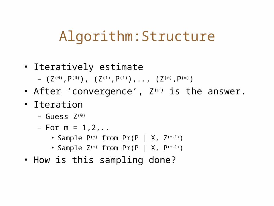
Algorithm:Structure

• Iteratively estimate – (Z(0),P(0)), (Z(1),P(1)),.., (Z(m),P(m))

• After ‘convergence’, Z(m) is the answer.• Iteration

– Guess Z(0)

– For m = 1,2,..• Sample P(m) from Pr(P | X, Z(m-1))• Sample Z(m) from Pr(P | X, P(m-1))

• How is this sampling done?

Example

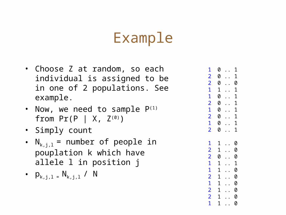
• Choose Z at random, so each individual is assigned to be in one of 2 populations. See example.

• Now, we need to sample P(1) from Pr(P | X, Z(0))

• Simply count

• Nk,j,l = number of people in pouplation k which have allele l in position j

• pk,j,l = Nk,j,l / N

0 .. 10 .. 10 .. 01 .. 10 .. 10 .. 10 .. 10 .. 10 .. 10 .. 1

1 .. 01 .. 00 .. 01 .. 11 .. 01 .. 01 .. 01 .. 01 .. 01 .. 0

1221121212

1221121221

Example

• Nk,j,l = number of people in population k which have allele l in position j

• pk,j,l = Nk,j,l / N1,1,*

• N1,1,0 = 4• N1,1,1 = 6• p1,1,0 = 4/10• p1,2,0 = 4/10 • Thus, we can sample P(m)

0 .. 10 .. 10 .. 01 .. 10 .. 10 .. 10 .. 10 .. 10 .. 10 .. 1

1 .. 01 .. 00 .. 01 .. 11 .. 01 .. 01 .. 01 .. 01 .. 01 .. 0

1221121212

1221121221

Sampling Z

• Pr[Z1 = 1] = Pr[”01” belongs to population 1]?

• We know that each position should be in linkage equilibrium and independent.

• Pr[”01” |Population 1] = p1,1,0 * p1,2,1

=(4/10)*(6/10)=(0.24)

• Pr[”01” |Population 2] = p2,1,0 * p2,2,1 = (6/10)*(4/10)=0.24

• Pr [Z1 = 1] = 0.24/(0.24+0.24) = 0.5

Sampling

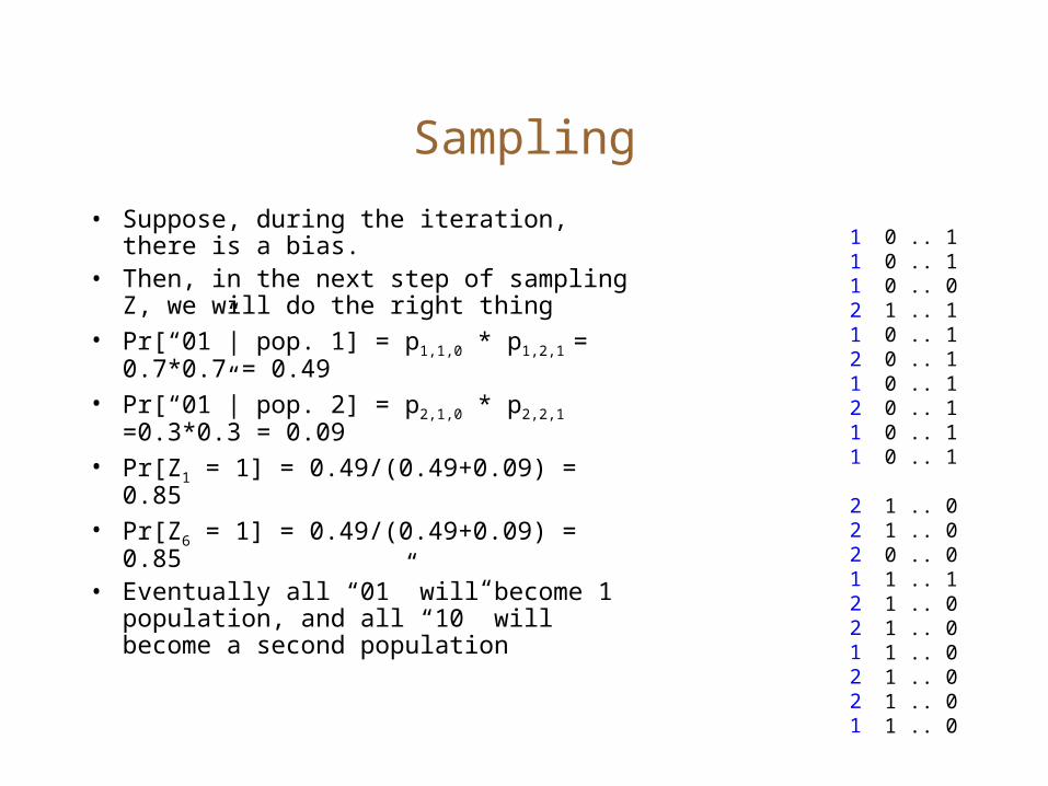
• Suppose, during the iteration, there is a bias.

• Then, in the next step of sampling Z, we will do the right thing

• Pr[“01”| pop. 1] = p1,1,0 * p1,2,1 = 0.7*0.7 = 0.49

• Pr[“01”| pop. 2] = p2,1,0 * p2,2,1

=0.3*0.3 = 0.09• Pr[Z1 = 1] = 0.49/(0.49+0.09) = 0.85• Pr[Z6 = 1] = 0.49/(0.49+0.09) = 0.85• Eventually all “01” will become 1

population, and all “10” will become a second population

0 .. 10 .. 10 .. 01 .. 10 .. 10 .. 10 .. 10 .. 10 .. 10 .. 1

1 .. 01 .. 00 .. 01 .. 11 .. 01 .. 01 .. 01 .. 01 .. 01 .. 0

1112121211

2221221221

Population Structure

• 377 locations (loci) were sampled in 1000 people from 52 populations.

• 6 genetic clusters were obtained, which corresponded to 5 geographic regions (Rosenberg et al. Science 2003)

AfricaEurasia East Asia

America

Oce

ania

Other topics

Protein SequenceAnalysis

Sequence Analysis

Gene Finding

Assembly

ncRNA

GenomicAnalysis/Pop. Genetics

ncRNA gene finding

• Gene is transcribed but not translated.• What are the clues to non-coding genes?

– Look for signals selecting start of transcription and translation. Non coding genes are transcribed by Pol III

– Non-coding genes have structure. Look for genomic sequences that fold into an RNA structure

• Structure: Given a sequence, what is the structure into which it can fold with minimum energy?

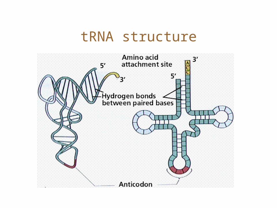
tRNA structure

RNA structure: Basics

• Key: RNA is single-stranded. Think of a string over 4 letters, AC,G, and U. • The complementary bases form pairs.• Base-pairing defines a secondary structure. The base-pairing is usually non-crossing.

RNA structure: pseudoknots

Sometimes, unpaired bases in loops form ‘crossing pairs’. These are pseudoknots

Transcript profiling

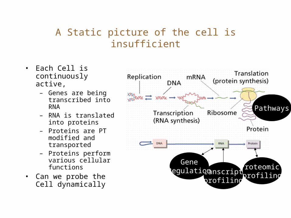
A Static picture of the cell is insufficient

• Each Cell is continuously active, – Genes are being

transcribed into RNA– RNA is translated into

proteins– Proteins are PT

modified and transported

– Proteins perform various cellular functions

• Can we probe the Cell dynamically

GeneRegulation Proteomic

profiling

Pathways

Gene expression

• The expression of transcripts and protein in the cell is not static. It changes in response to signals.

• The expression can be measured using micro-arrays.

• What causes the change in expression?

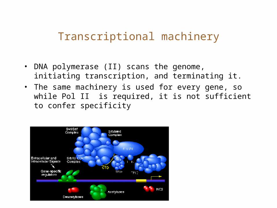
Transcriptional machinery

• DNA polymerase (II) scans the genome, initiating transcription, and terminating it.

• The same machinery is used for every gene, so while Pol II is required, it is not sufficient to confer specificity

TF binding

• Other transcription factors interact with the core machinery and upstream DNA to provide specificity.

• TFs bind to TF binding sites which are clustered in upstream enhancer and promoter elements.

• The enhancer elements may be located many kb upstream of the core-promoter

Upstream elements

Transcription factors

TF binding sites• TF binding sites are

weak signal (about 10 bp with 5bp conserved)

• If two genes are co-regulated, they are likely to share binding sites

• Discovery of binding site motifs is an important research problem.

TGAGGAG

TCAGGAG

TCAGGTG

TGAGGTG

TCAGGTG

g1

g2

g3

g4

g5

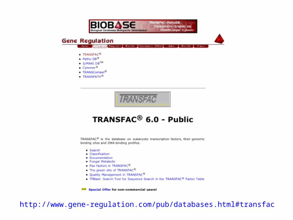
http://www.gene-regulation.com/pub/databases.html#transfac

Discovering TF binding sites

• Identification of these TF binding sites/switches is critical.

• Requires identification of co-regulated genes (genes containing the same set of switches).

• How do we find co-regulated genes?

Idea1: Use orthologous genes from different species

ACGGCAGCTCGCCGCCGCGC||||| || ||||||| ||ACGGC-GGGCGCCGCCCCGC

ACGGCAGCTCGCCGCCGC-C| || | ||||||| | AGTGC-GGGCGCCGCCTCAT

ACGGC-GC-TCGCCGCCGCGC| | | || | | AT-ACGAAGTAGCGG-ATGGT

1. The species are too close (EX: humans and chimps). Binding & non-binding sites are both conserved.

2. The species are distant. Binding sites are conserved but not other sequence.

3. The species are very distant. Even binding sites are not conerved. The genes have alternative regulators.

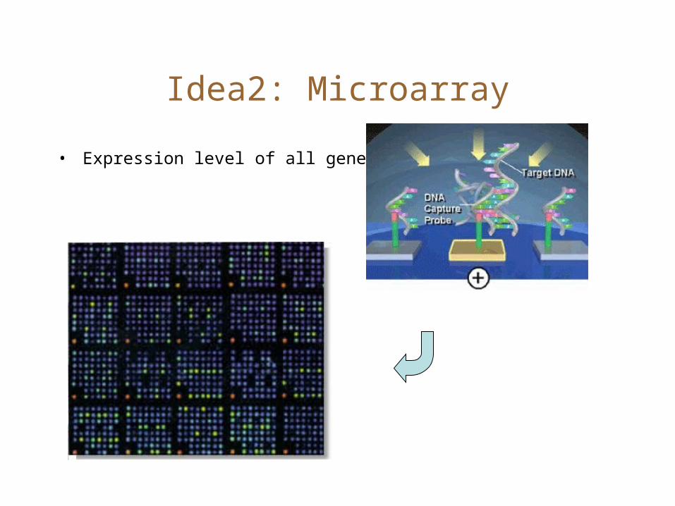
Idea2: Microarray

• Expression level of all genes

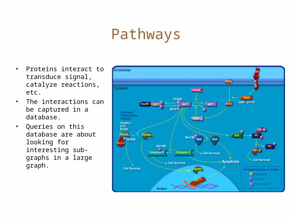
Pathways

• Proteins interact to transduce signal, catalyze reactions, etc.

• The interactions can be captured in a database.

• Queries on this database are about looking for interesting sub-graphs in a large graph.

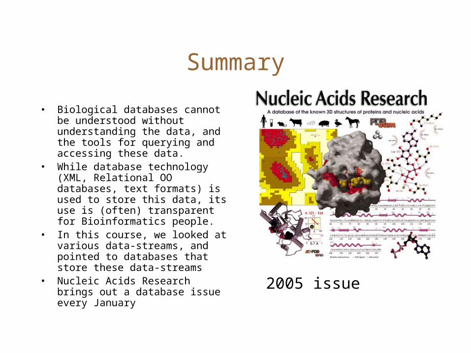
Summary

• Biological databases cannot be understood without understanding the data, and the tools for querying and accessing these data.

• While database technology (XML, Relational OO databases, text formats) is used to store this data, its use is (often) transparent for Bioinformatics people.

• In this course, we looked at various data-streams, and pointed to databases that store these data-streams

• Nucleic Acids Research brings out a database issue every January

2005 issue