CSE.0002 Introduction to Computational Science and ...

CSE.0002Introduction to Computational Science and

EngineeringClass notes

TeamDraft October 21, 2020

Preface

What is Computational Science and Engineering (CSE)? In com-puter science, we study algorithms for tasks like sorting a list, partitioning agraph, finding the shortest path, and many more. In CSE, we first look to thesciences (physics, chemistry, biology, Earth sciences, social sciences,. . . ), findthe equations that describe some phenomenon, and then study the algorithmsthat solve those equations or manipulate them somehow. These mathemati-cal equations are called models, and they include Newton’s law (F=ma), massbalance and reaction rates for chemical or biological compounds, the laws ofelectromagnetism, etc. They often involve implicit relationships like differ-ential equations that still need to be solved with algorithms to reveal usefulinformation. Setting up models and solving them is universal and powerful –all engineering and science fields use models from robotics to climate science,atomic to planetary motion, epidemiology, material science to electrical en-gineering, and so on. CSE also enables optimization, control, data fitting,and uncertainty quantification for the systems described by those models.

As a discipline, CSE typically involves scientific and engineering aspects(where the models come from), analytical aspects (how to understand themodels mathematically), and computational aspects (how to deal with themodels on a computer.) The emphasis on these notes is mostly on the thirdaspect, computation.

Contents:

Part 1: Models and Simulation

• Introduction to Initial Value Problems (IVP), the exponential so-lution, numerical methods for IVP.

• Systems of equations, elimination, implicit methods for linear sys-tems of IVP.

3

4

• Nonlinear models, root-finding and Newton’s method, implicitmethods for nonlinear IVP.

Part 2: Optimization and Control

• Constrained and unconstrained formulations

• Classification of minima

• Iterative methods

Part 3: Uncertainty Quantification

• Probability: random variable, distribution, moments, conditionalprobabilities

• Estimation of the mean and standard deviation, confidence inter-vals

• Monte Carlo sampling

Many examples from mechanics (robotics, planetary motion, particle mo-tion, vehicle motion), chemistry, Earth and climate science, biology (epidemi-ology), etc.

Chapter 1

Introduction to Initial ValueProblems

1.1 Time-dependent phenomena and rates of

change

A major objective of this subject is to introduce key concepts behind compu-tational algorithms used to simulate phenomena that depend on time. Timerates of change, not surprisingly, play an important role in modeling time-dependent phenoma.

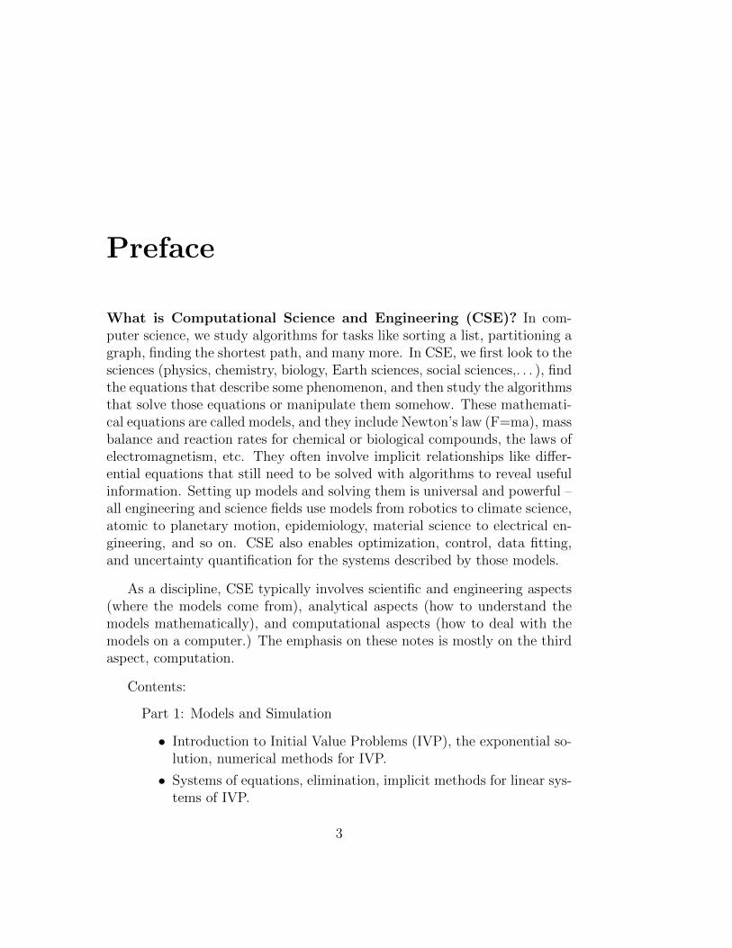
Example 1. Consider the deceleration to rest of a car that is initially movingat 90 km/hr = 25 m/s. Figure 1.1 shows an example of how the car’s positionx(t), velocity V (t), and acceleration a(t) might behave during the deceleration.The velocity is defined as the time rate of change of the position,

V =dx

dt

Graphically, V (t) is the slope at time t of the x(t) plot. And similarly, theacceleration is defined as the time rate of change of the velocity,

a =dV

dt

The motion shown in the plot is one in which the acceleration is small ini-tially, and then increases in magnitude during the middle of the deceleration,and again becomes small (in fact 0) at the end of the motion. As with therelationship of V to x, a(t) is the slope at time t of the plot of V (t).

5

6 CHAPTER 1. INTRODUCTION TO INITIAL VALUE PROBLEMS

0

50

100

150x

(m)

0

5

10

15

20

25

V (m

/s)

0 2 4 6 8 10 12t (s)

3

2

1

0

a (m

/s^2

)

Figure 1.1: Position, velocity and acceleration of a vehicle braking from 25m/s to rest.

Indeed, the notation dvdt

for the derivative of v with respect to t is sugges-tive of a ratio of differences:

dv

dt(t) ' ∆v

∆t=v(t+ ∆t)− v(t)

(t+ ∆t)− t=v(t+ ∆t)− v(t)

∆t, (1.1)

and the ' sign becomes an equality (=) in the limit when the small timeincrement ∆t is taken to zero. We might also use v′(t) or v(t) to denote thederivative of v with respect to t at time t).

1.2 Models of Time-dependent Phenomena

The mathematical models used to describe time-dependent phenomena inNature and social systems are frequently differential equations, i.e., rela-tionships between functions and their derivatives.

1.2. MODELS OF TIME-DEPENDENT PHENOMENA 7

Where do models involving derivatives come from? The most importantexample is perhaps ~F = m~a, Newton’s second law, that we have alreadyencountered. Here the basic quantity is the position ~x(t) of a particle or anobject as a function of time t. In general, ~x(t) = (x1(t), x2(t), x3(t)) is avector in 3 dimensions for each time t, but there are also cases where we onlyconsider two, or one component of x(t) at a time (and we might still denotethose by x(t) when convenient). Then the velocity vector ~v(t) is the timederivative of ~x(t), and the acceleration vector ~a(t) is the time derivative of~v(t):

~v(t) =d~x

dt(t), ~a(t) =

d~v

dt(t) =

d2~x

dt2(t).

The force vector ~F acting on the object at x(t) is either given as a functionof time, or is itself a function of x and/or v. Either way, “F = ma” becomesa differential equation.

More generally, mathematical models involving derivatives range fromtrustworthy elegant theories (like Newton’s laws of gravity; or Euler’s equa-tion of fluid dynamics; or Maxwell’s laws of electromagnetism; or Einstein’slaws of gravity; or Schrodinger’s law of quantum mechanics,...) to ad-hocrelationships that imperfectly quantify some aspects of a phenomenon (likeaveraged models of viral spread; or models of average concentration of chem-icals; or models of temperature of an object; or macroscopic models of flowsin porous media; or models for option pricing in investment banking,...). Asyou can see, the list is long! We will encounter many of them throughout thenotes. But all these example have in common that they involve differentialequations that need to be solved. CSE offers the common knowledge neededto tackle (almost) all of them.

In the remainder of this section, we consider a few examples of such modeldifferential equations.

1.2.1 Skydiving

The motion of a sky diver can be modeled using “F=ma”. Let V (t) be thevelocity oriented downward (in the direction of gravity). Then, a = dV/dt isthe acceleration downward. The force F is also defined as oriented downwardand is a combination of gravity and aerodynamic drag. The aerodynamicdrag, D, opposes the velocity (and thus acts upward). Thus, F = mg − D


and the model differential equation can be written,

mdV

dt= mg −D

The drag on an object (in this case, a skydiver) is frequently estimated usinga drag coefficient CD as follows,

CD =D

12ρaV 2Aref

(1.2)

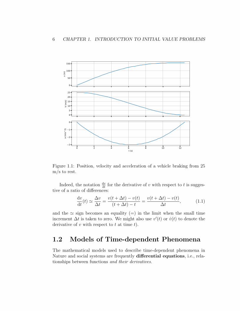
where ρa is the density of the air and Aref is a reference area which is relatedin some way to the geometry of the object. Drag coefficients (which are non-dimensional) can frequently be estimated for shapes based upon knowledgeof CD for similar (or the same) shapes. We will consider a sky diver in threeorientations:

• Spread eagle: in this high drag case, typically the reference area ischosen as the area of the skydiver as viewed from below. So, for atypical human, this would be about Aref ≈ 0.64 m2. And the CD ≈ 1.

• Arrow: in this low drag case, the diver orients pointed downward.Traditionally, the reference area for this orientation is chosen as thesame as the spread eagle. So, Aref ≈ 0.64 m2. The drag coefficient isabout a factor of ten less in this orientation, CD ≈ 0.1.

• Ball: in this case, the diver rolls into a compact ball shape. The refer-ence area is usually the cross-sectional area of the “ball”, which wouldbe approximately 0.2 m2. And the CD ≈ 0.4.

Independent of the specific orientation, the drag can be expressed usingthe CD as,

D =1

2ρaV

2ArefCD

Finally, combining this gives the form of the model equation as,

mdV

dt= mg − 1

2ρaV

2ArefCD (1.3)

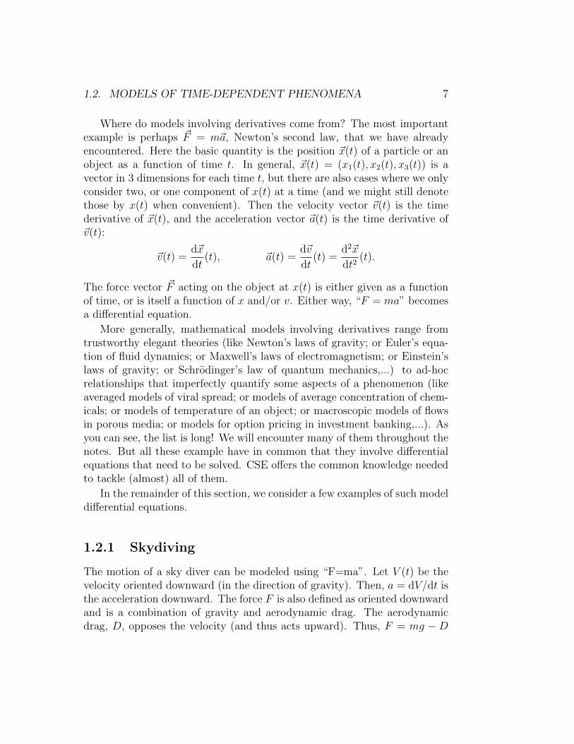
In Figure 1.3, the velocity evolution V (t) is shown for the three orientationsusing the following values for the other parameters,

V (0) = 0 ρa = 1 kg/m3 g = 9.81 m/s2 m = 80 kg


Figure 1.2: Skydiver in spread eagle and arrow positions.

0 20 40 60 80 100t (s)

0

20

40

60

80

100

120

140

160

V (m

/s)

Skydiver velocity vs. timeeagleballarrow

Figure 1.3: Skydiver velocity V (t) in three different positions


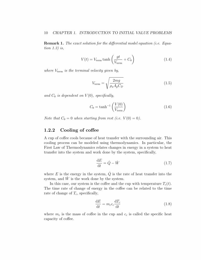
Remark 1. The exact solution for the differential model equation (i.e. Equa-tion 1.3) is,

V (t) = Vterm tanh

(gt

Vterm

+ C0

)(1.4)

where Vterm is the terminal velocity given by,

Vterm =

√2mg

ρaApCD

(1.5)

and C0 is dependent on V (0), specifically,

C0 = tanh−1

(V (0)

Vterm

)(1.6)

Note that C0 = 0 when starting from rest (i.e. V (0) = 0).

1.2.2 Cooling of coffee

A cup of coffee cools because of heat transfer with the surrounding air. Thiscooling process can be modeled using thermodynamics. In particular, theFirst Law of Thermodynamics relates changes in energy in a system to heattransfer into the system and work done by the system, specifically,

dE

dt= Q− W (1.7)

where E is the energy in the system, Q is the rate of heat transfer into thesystem, and W is the work done by the system.

In this case, our system is the coffee and the cup with temperature Tc(t).The time rate of change of energy in the coffee can be related to the timerate of change of Tc, specifically,

dE

dt= mccc

dTcdt

(1.8)

where mc is the mass of coffee in the cup and cc is called the specific heatcapacity of coffee.


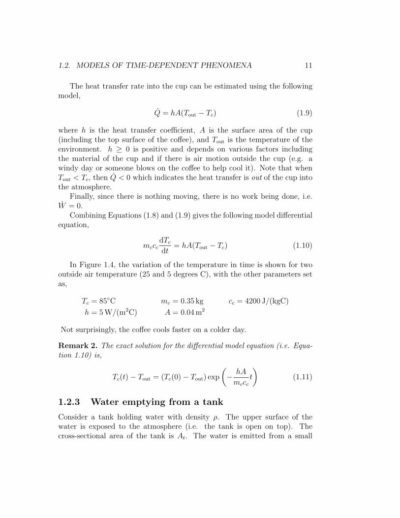
The heat transfer rate into the cup can be estimated using the followingmodel,

Q = hA(Tout − Tc) (1.9)

where h is the heat transfer coefficient, A is the surface area of the cup(including the top surface of the coffee), and Tout is the temperature of theenvironment. h ≥ 0 is positive and depends on various factors includingthe material of the cup and if there is air motion outside the cup (e.g. awindy day or someone blows on the coffee to help cool it). Note that whenTout < Tc, then Q < 0 which indicates the heat transfer is out of the cup intothe atmosphere.

Finally, since there is nothing moving, there is no work being done, i.e.W = 0.

Combining Equations (1.8) and (1.9) gives the following model differentialequation,

mcccdTcdt

= hA(Tout − Tc) (1.10)

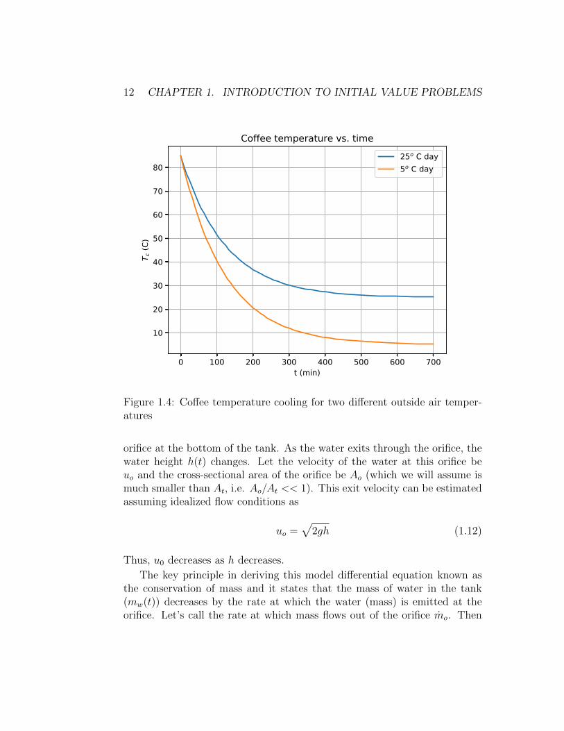
In Figure 1.4, the variation of the temperature in time is shown for twooutside air temperature (25 and 5 degrees C), with the other parameters setas,

Tc = 85◦C mc = 0.35 kg cc = 4200 J/(kgC)

h = 5 W/(m2C) A = 0.04 m2

Not surprisingly, the coffee cools faster on a colder day.


Tc(t)− Tout = (Tc(0)− Tout) exp

(− hA

mccct

)(1.11)

1.2.3 Water emptying from a tank

Consider a tank holding water with density ρ. The upper surface of thewater is exposed to the atmosphere (i.e. the tank is open on top). Thecross-sectional area of the tank is At. The water is emitted from a small


0 100 200 300 400 500 600 700t (min)

10

20

30

40

50

60

70

80

T c (C

)Coffee temperature vs. time

25o C day5o C day

Figure 1.4: Coffee temperature cooling for two different outside air temper-atures

orifice at the bottom of the tank. As the water exits through the orifice, thewater height h(t) changes. Let the velocity of the water at this orifice beuo and the cross-sectional area of the orifice be Ao (which we will assume ismuch smaller than At, i.e. Ao/At << 1). This exit velocity can be estimatedassuming idealized flow conditions as

uo =√

2gh (1.12)

Thus, u0 decreases as h decreases.

The key principle in deriving this model differential equation known asthe conservation of mass and it states that the mass of water in the tank(mw(t)) decreases by the rate at which the water (mass) is emitted at theorifice. Let’s call the rate at which mass flows out of the orifice mo. Then


At

Ao

u0

h(t)

g

x

y

Figure 1.5: Water emptying from a tank

conservation of mass gives,

dmw

dt= −mo (1.13)

At any instant, the mass of water in the tank, mw(t) is equal to thevolume of water Volw(t) and the density ρ through mw = ρVolw. The watervolume is simply Ath. Thus,

mw(t) = ρVolw(t) = ρAth(t) (1.14)

The mass flow rate out of the orifice can be shown to be mo = ρAouowhich upon substitution of Equation (1.12) gives,

mo = ρAo

√2gh (1.15)

Finally, substituting Equations (1.14) and (1.12) into Equation (1.13)gives the model differential equation,

Atdh

dt= −Ao

√2gh (1.16)

Note that the left-hand side arises because ρ and At do not depend on time,and so differentiating ρAth with respect to time gives ρAtdh/dt. Also notethat the density (maybe somewhat surprisingly) is eliminated from this modelequation. In other words, the flow of water out of the tank does not dependon its density!


0 25 50 75 100 125 150 175t (s)

0.04

0.06

0.08

0.10

0.12

0.14

h (m

)Water height vs. time

ModelExperiment

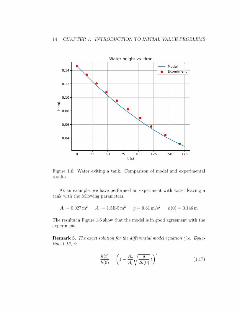
Figure 1.6: Water exiting a tank. Comparison of model and experimentalresults.

As an example, we have performed an experiment with water leaving atank with the following parameters,

At = 0.027 m2 Ao = 1.5E-5 m2 g = 9.81 m/s2 h(0) = 0.146 m

The results in Figure 1.6 show that the model is in good agreement with theexperiment.


h(t)

h(0)=

(1− Ao

At

√g

2h(0)t

)2

(1.17)

1.3. INITIAL VALUE PROBLEMS 15

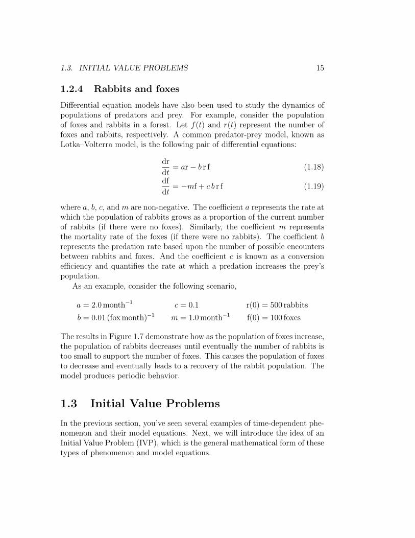
1.2.4 Rabbits and foxes

Differential equation models have also been used to study the dynamics ofpopulations of predators and prey. For example, consider the populationof foxes and rabbits in a forest. Let f(t) and r(t) represent the number offoxes and rabbits, respectively. A common predator-prey model, known asLotka–Volterra model, is the following pair of differential equations:

dr

dt= ar− b r f (1.18)

df

dt= −mf + c b r f (1.19)

where a, b, c, and m are non-negative. The coefficient a represents the rate atwhich the population of rabbits grows as a proportion of the current numberof rabbits (if there were no foxes). Similarly, the coefficient m representsthe mortality rate of the foxes (if there were no rabbits). The coefficient brepresents the predation rate based upon the number of possible encountersbetween rabbits and foxes. And the coefficient c is known as a conversionefficiency and quantifies the rate at which a predation increases the prey’spopulation.

As an example, consider the following scenario,

a = 2.0 month−1 c = 0.1 r(0) = 500 rabbits

b = 0.01 (fox month)−1 m = 1.0 month−1 f(0) = 100 foxes

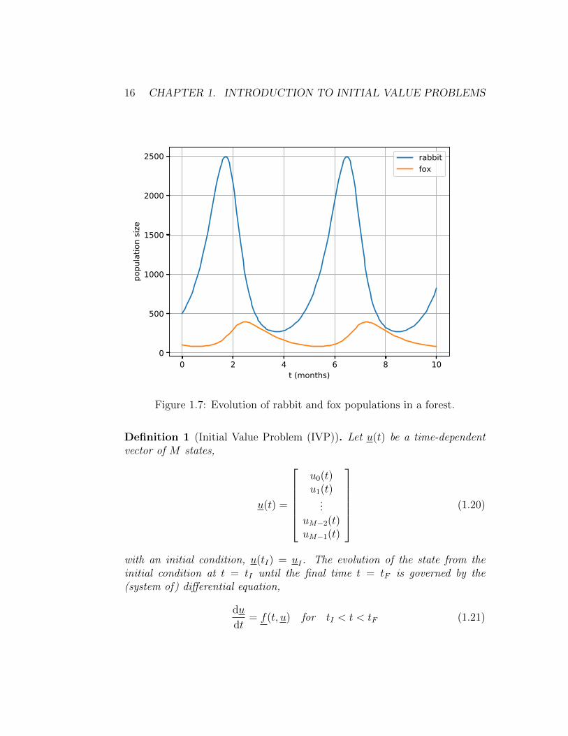
The results in Figure 1.7 demonstrate how as the population of foxes increase,the population of rabbits decreases until eventually the number of rabbits istoo small to support the number of foxes. This causes the population of foxesto decrease and eventually leads to a recovery of the rabbit population. Themodel produces periodic behavior.

1.3 Initial Value Problems

In the previous section, you’ve seen several examples of time-dependent phe-nomenon and their model equations. Next, we will introduce the idea of anInitial Value Problem (IVP), which is the general mathematical form of thesetypes of phenomenon and model equations.


0 2 4 6 8 10t (months)

0

500

1000

1500

2000

2500

popu

latio

n siz

e

rabbitfox

Figure 1.7: Evolution of rabbit and fox populations in a forest.

Definition 1 (Initial Value Problem (IVP)). Let u(t) be a time-dependentvector of M states,

u(t) =

u0(t)u1(t)

...uM−2(t)uM−1(t)

(1.20)

with an initial condition, u(tI) = uI . The evolution of the state from theinitial condition at t = tI until the final time t = tF is governed by the(system of) differential equation,

du

dt= f(t, u) for tI < t < tF (1.21)

1.3. INITIAL VALUE PROBLEMS 17

Remark 4. When M = 1, we refer to the problem as a scalar IVP. Forconvenience and clarity, we drop the underline notation and write the scalarIVP as,

du

dt= f(t, u) for tI < t < tF (1.22)

with u(tI) = uI .

Remark 5. While the IVP description above is for a range of time tI < t <tF , often we may not know a precise final time. Rather, we are interestedin solving the problem until the time when some event occurs. For example,in the coffee cooling, perhaps we want to know how long we have until thetemperature drops to Tc = 70◦C. Or, for the water tank problem, we maywant to run the simulation until the tank is completely empty. In eithercase, we will not know ahead of time how long it will take (that’s why we arerunning the simulation after all)! When this situation occurs, we will justinclude a check within our computer code to see if some condition has beenmet. When it is met (e.g. the coffee temperature has reached 70◦C), thenthe computation will be stopped.

For simplicity in most of these notes, we will assume that tF is known.

1.3.1 Skydiving

For the skydiving example in Section 1.2.1, dividing Equation (1.3) by mgives

dV

dt= g − 1

2

ρaV2ArefCD

m(1.23)

which in terms of the general IVP form gives a scalar (M = 1) system ofequation with

u = V f = g − 1

2

ρau2ArefCD

m(1.24)

1.3.2 Cooling of coffee

For the coffee cooling example in Section 1.2.2, dividing Equation (1.10) bymccc gives

dTcdt

=hA

mccc(Tout − Tc) (1.25)



u = Tc f =hA

mccc(Tout − u) (1.26)

1.3.3 Water emptying from a tank

For the water tank example in Section 1.2.3, dividing Equation (1.16) by At

gives

dh

dt= −Ao

At

√2gh (1.27)


u = h f = −Ao

At

√2gu (1.28)

1.3.4 Rabbits and foxes

For the predator-prey example in Section 1.2.4, Equations (1.18) and (1.19)are already in the IVP general form. This M = 2 system of equations has,

u0 = r f0 = au0 − b u0 u1 (1.29)

u1 = f f1 = −mu1 + c b u0 u1 (1.30)

1.4 Linear scalar IVP and exponential solu-

tion

The behavior of a linear scalar (M = 1) IVP provides useful insight intothe behavior of much more complex systems of equations. Further, manyphenomena can be described by a linear scalar IVP. The mean of linear isthe f is at most a linear function of u. For the scalar M = 1 case, considerthe following linear differential model equation,

du

dt= λu (1.31)

1.4. LINEAR SCALAR IVP AND EXPONENTIAL SOLUTION 19

where λ is a constant (i.e. independent of time). Thus, for this linear scalarIVP, f = λu.

Recall that the derivative of the exponential function exp(λt) is λ exp(λt),i.e.

d

dt[exp(λt)] = λ exp(λt)

Comparing this to Equation (1.31), we see that the solution to that equationis,

u(t) = uI exp(λt) (1.32)

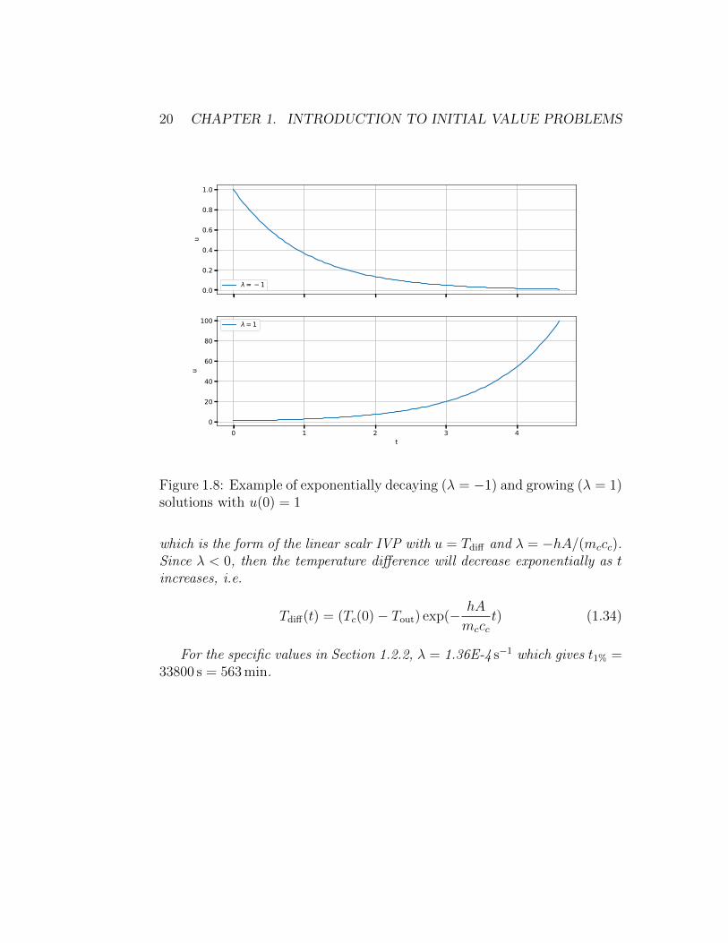
For λ < 0, then as t increases, the state u(t) decreases in magnitude. Thisis known as an exponentially decaying solution. And vice-cersa, for λ > 0,the state u(t) increases in magnitude as t increases. This is known as anexponentially growing solution. An example of these solutions is shown forλ = −1 and λ = 1 with u(0) = 1 in Figure 1.8.

A useful idea is that λ is a rate constant (units of 1/time) and we canthink of 1/λ as a time scale. For example, in the case of an exponentiallydecaying solution, let t1% be the time when the state will be 1% of its initialcondition. This occurs when λt = −4.6. (i.e. exp(−4.6) = 0.01). Thus,t1% = 4.6/|λ| for a decaying solution. For an exponentially growing solution,the same time scale will give the time at which the state was been amplifiedby a factor of 100.

Example 2 (Coffee cooling in a cup). Recall the model equation for coffeecooling in a cup as given in Equation (1.25). By change the state variableto be the difference in temperature between Tc and Tout, we can recover thelinear scalar IVP of Equation (1.31). Define Tdiff(t) ≡ Tc(t) − Tout. Notethat,

dTdiff

dt=

dTcdt

Then Equation (1.25) can be written as,

dTdiff

dt= − hA

mcccTdiff (1.33)


0.0

0.2

0.4

0.6

0.8

1.0u

= 1

0 1 2 3 4t

0

20

40

60

80

100

u

= 1

Figure 1.8: Example of exponentially decaying (λ = −1) and growing (λ = 1)solutions with u(0) = 1

which is the form of the linear scalr IVP with u = Tdiff and λ = −hA/(mccc).Since λ < 0, then the temperature difference will decrease exponentially as tincreases, i.e.

Tdiff(t) = (Tc(0)− Tout) exp(− hA

mccct) (1.34)

For the specific values in Section 1.2.2, λ = 1.36E-4 s−1 which gives t1% =33800 s = 563 min.

Chapter 2

Introduction to Discretizationof IVP

2.1 Discretization

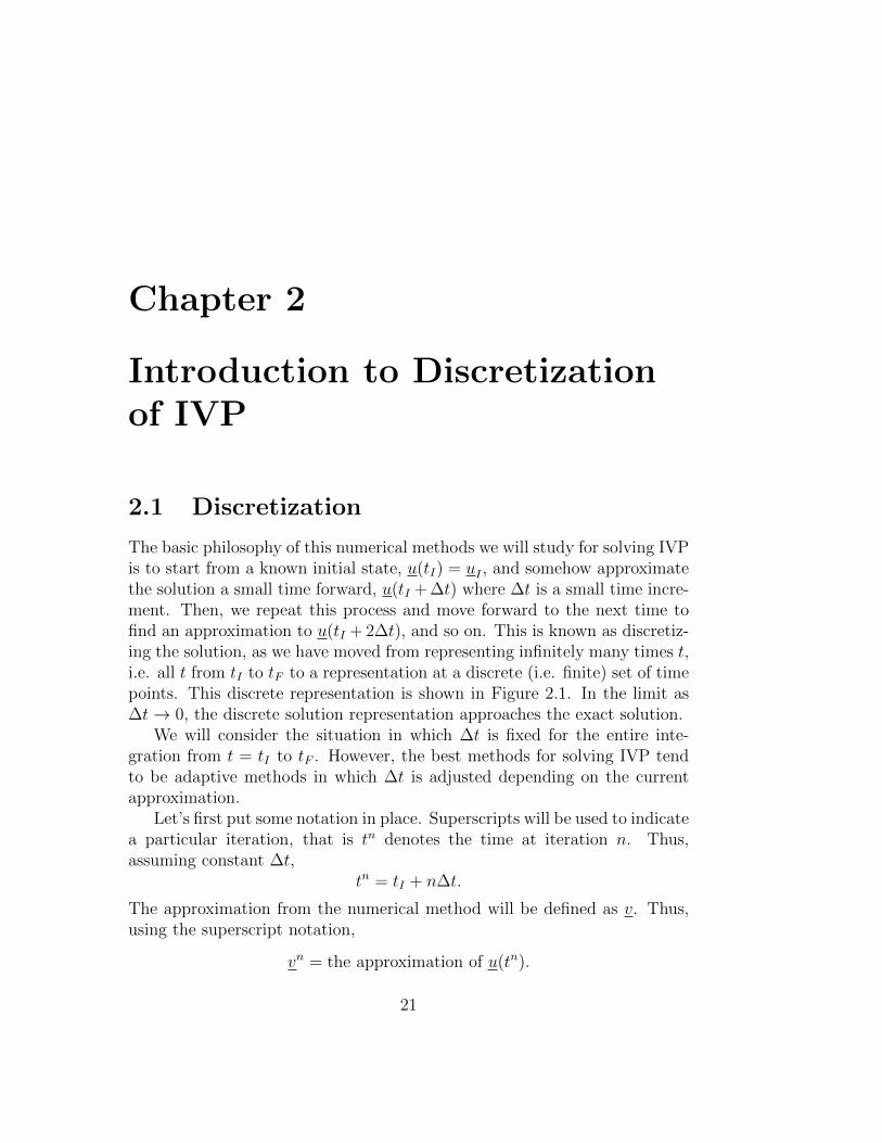
The basic philosophy of this numerical methods we will study for solving IVPis to start from a known initial state, u(tI) = uI , and somehow approximatethe solution a small time forward, u(tI + ∆t) where ∆t is a small time incre-ment. Then, we repeat this process and move forward to the next time tofind an approximation to u(tI + 2∆t), and so on. This is known as discretiz-ing the solution, as we have moved from representing infinitely many times t,i.e. all t from tI to tF to a representation at a discrete (i.e. finite) set of timepoints. This discrete representation is shown in Figure 2.1. In the limit as∆t→ 0, the discrete solution representation approaches the exact solution.

We will consider the situation in which ∆t is fixed for the entire inte-gration from t = tI to tF . However, the best methods for solving IVP tendto be adaptive methods in which ∆t is adjusted depending on the currentapproximation.

Let’s first put some notation in place. Superscripts will be used to indicatea particular iteration, that is tn denotes the time at iteration n. Thus,assuming constant ∆t,

tn = tI + n∆t.

The approximation from the numerical method will be defined as v. Thus,using the superscript notation,

vn = the approximation of u(tn).

21

22 CHAPTER 2. INTRODUCTION TO DISCRETIZATION OF IVP

°A. uL↳)=u°

une ult , + not)i÷÷# tbt ft

n n . . . .

Figure 2.1: Discrete representation of the exact solution in which u(t) issampled at tn = tI + n∆t giving un = u(tn)

2.2 Forward Euler method

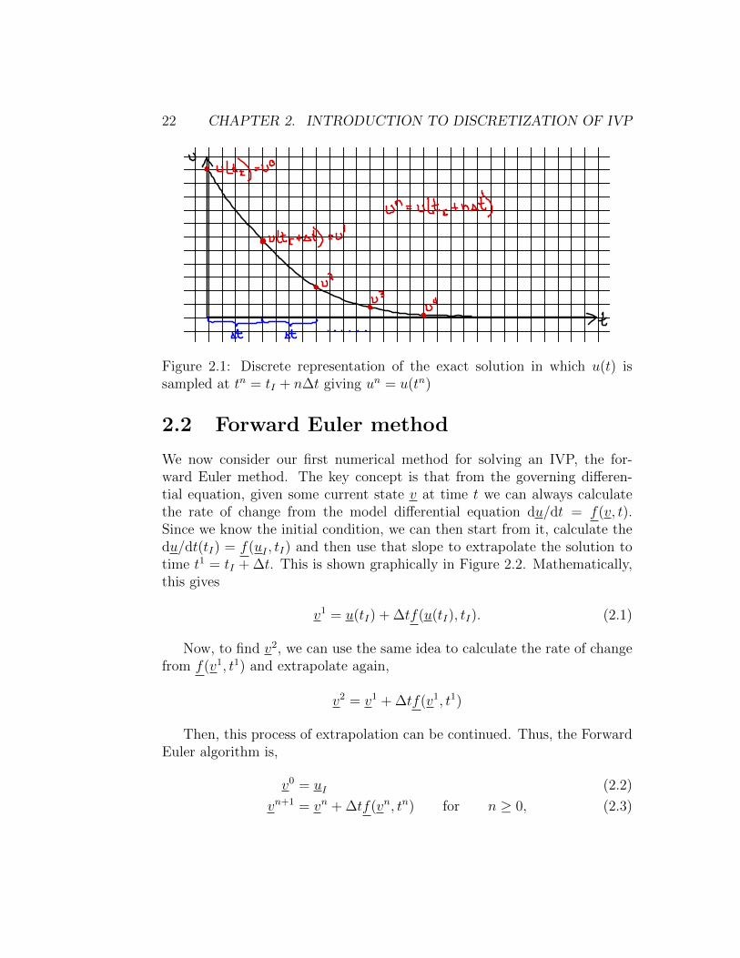
We now consider our first numerical method for solving an IVP, the for-ward Euler method. The key concept is that from the governing differen-tial equation, given some current state v at time t we can always calculatethe rate of change from the model differential equation du/dt = f(v, t).Since we know the initial condition, we can then start from it, calculate thedu/dt(tI) = f(uI , tI) and then use that slope to extrapolate the solution totime t1 = tI + ∆t. This is shown graphically in Figure 2.2. Mathematically,this gives

v1 = u(tI) + ∆tf(u(tI), tI). (2.1)

Now, to find v2, we can use the same idea to calculate the rate of changefrom f(v1, t1) and extrapolate again,

v2 = v1 + ∆tf(v1, t1)

Then, this process of extrapolation can be continued. Thus, the ForwardEuler algorithm is,

v0 = uI (2.2)

vn+1 = vn + ∆tf(vn, tn) for n ≥ 0, (2.3)

2.2. FORWARD EULER METHOD 23

°£ u Lte) = u° =V

O= uI

une uLt,+ not)

"""fi÷÷÷# t

bt ftn n . . . .

Figure 2.2: Forward Euler method

Example 3 (Forward Euler simulation of coffee cooling). The script belowis a Forward Euler simulation of coffee cooling. The resulting plot is shownin Figure 2.3.

######### BEGINNING OF PYTHON SCRIPT #########

import matplotlib.pyplot as plt

import math

mc = 0.35 # kg

cc = 4200.0 # J / (kg C)

h = 5.0 # W/(m^2 C)

A = 0.04 # m^2

Tout = 25.0 # C

TcI = 85.0 # Initial temperature of coffee (C)

tFmin = 700.0 # final time to simulate to (min)

dtmin = 5e1 # time increment to give solutions at (min)

# Convert times to seconds

tF = tFmin*60

dt = dtmin*60


# Sets initial condition

t = [0]

v = [TcI]

# Loop from from t=0 to t>=tF

tn = t[0]

vn = v[0]

while (tn<tF):

# Calculate forcing

fn = h*A/(mc*cc)*(Tout - vn)

# Update solution and time

vn1 = vn + dt*fn

tn1 = tn + dt

# Append to v and t

v.append(vn1)

t.append(tn1/60) # store time in minutes

# Set vn and tn for next iteration

vn = vn1

tn = tn1

# Calculate exact solution and error

u = []

e = []

lam = -h*A/(mc*cc)

for n in range(len(t)):

ts = t[n]*60

un = Tout + (TcI-Tout)*math.exp(lam*ts)

en = abs(v[n]-un)

u.append(un)

e.append(en)

# Plot

2.3. ACCURACY AND CONVERGENCE 25

plt.subplot(2,1,1)

plt.scatter(t,v,marker=’o’,label=’numerical’)

plt.ylabel(’$T_c$ (C)’)

plt.grid(True)

plt.scatter(t,u,marker=’x’,label=’exact’)

plt.legend()

plt.subplot(2,1,2)

plt.scatter(t,e,marker=’o’)

plt.xlabel(’t (min)’)

plt.ylabel(’error (C)’)

plt.grid(True)

######### END OF PYTHON SCRIPT #########

2.3 Accuracy and Convergence

As the timestep is decreased, i.e. ∆t → 0, we would like our numericalmethod to better approximate the exact solution to the model equations.Let’s define the error in our approximation at timestep n to be:

en ≡ vn − u(tn) (2.4)

Since this is u(tn) is in general an M -dimensional vector of states, then soare vn and en. We can define the components of this error then,

enm = vnm − um(tn) (2.5)

for each m = 0 to M−1. Then, to measure the error for the entire simulation(i.e. over all timesteps), we’ll take the maximum magnitude,

(em)max = maxn|enm| (2.6)

Then, in terms of these error definitions, we desire that the maximumerror in each state goes to zero as ∆t→ 0. This concept is known as conver-gence and is stated mathematically as follows:


0 100 200 300 400 500 600 700t (min)

30

40

50

60

70

80

T c (C

)numericalexact

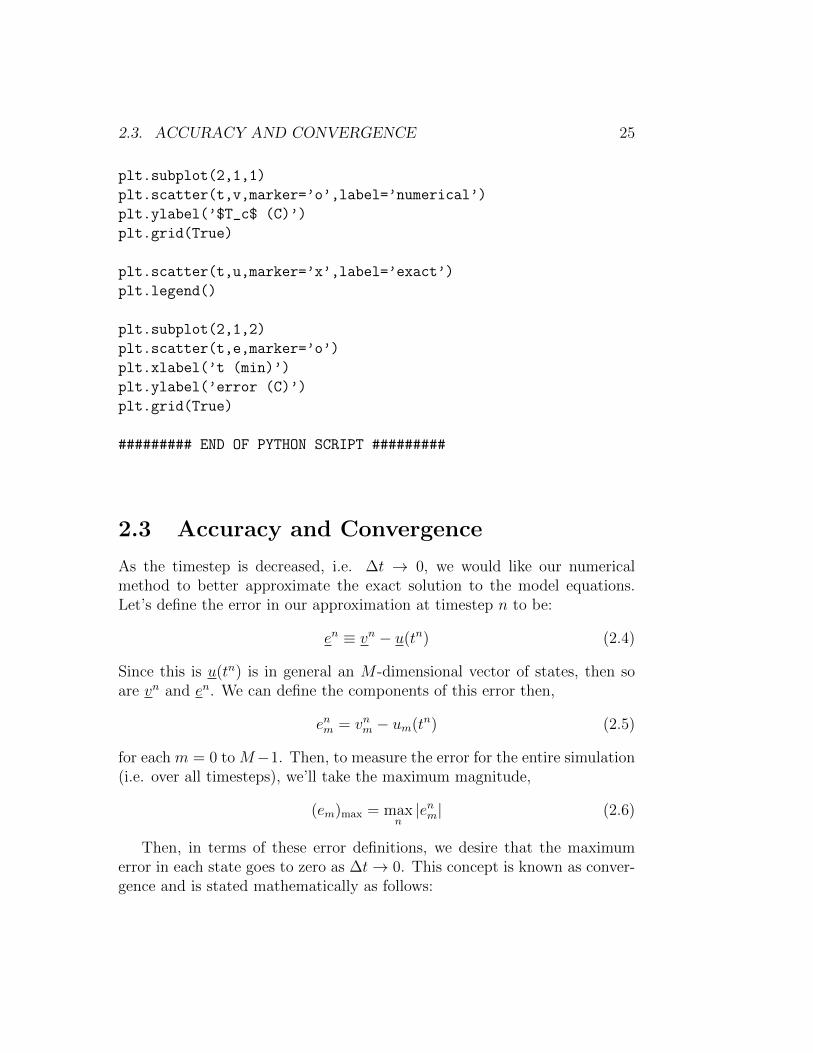
Figure 2.3: Forward Euler method applied to coffee cooling using ∆t = 50minutes.

Definition 2 (Convergence). A numerical method for an Initial Value Prob-lem is convergent from t = tI to tF is convergent if for all m,

(em)max → 0 as ∆t→ 0.

While convergence is a clear requirement for a good numerical method,the rate at which the method converges is also important. This rate is knownas the order of accuracy.

Definition 3 (Order of Accuracy). A method has an order of accuracy of pif, for all m,

(em)max = O(∆tp) as ∆t→ 0,

Some important comments:

2.4. RUNGE-KUTTA METHODS 27

• Theoretical proofs do exist for the order of accuracy of numerical meth-ods. However, that is beyond the scope of this introductory course.

• Typically, when a given numerical method is said to have a convergencerate p (e.g., the Forward Euler method is 1st-order accurate, i.e. p = 1)this assumes that the problem being solved is sufficiently smooth.

• The details on this issue of smoothness and accuracy are advancedtopics which we can’t cover here.

Example 4 (Accuracy of Forward Euler simulation of coffee cooling). Let’sconsider the error for the Forward Euler simulation of coffee cooling. Fig-ure 2.4 shows that the error decreases by about a factor of 10 for a factor of10 decrease in ∆t from 50 to 5 minutes. This would seem to indicate a firstorder (p = 1) method since the error seems proportion to ∆.

To see more certainly that Forward Euler is p = 1, we plot the maximumerror (emax) versus a range of ∆t in Figure 2.5. This plot is done using alog-log scale because the slope then is directly the observed order of accuracy.To see that this is true, recall that the definition of the order of accuracy saysthat,

emax = O(∆tp)

log emax = O(log(∆tp))

⇒ log emax = O(p log ∆t)

Thus, p is the slope of the log emax versus log ∆t plot. As can be seen inFigure 2.5, the slope is 1.

2.4 Runge-Kutta Methods

2.4.1 2nd order Runge-Kutta Method (RK2)

A popular second-order (p = 2) Runge-Kutta (RK2) method is known asthe modified Euler method. The basic idea is to attempt to estimate theslope du/dt at the middle of a timestep (i.e. at tn + ∆/2) and use thatestimated slope in the Forward Euler method. Specically, the modified Euler


0 100 200 300 400 500 600 700

30

40

50

60

70

80T c

(C)

t = 50 minnumericalexact

0 100 200 300 400 500 600 700t (min)

0

1

2

3

4

5

erro

r (C)

0 100 200 300 400 500 600 700

30

40

50

60

70

80

T c (C

)

t = 5 minnumericalexact

0 100 200 300 400 500 600 700t (min)

0.0

0.1

0.2

0.3

0.4

erro

r (C)

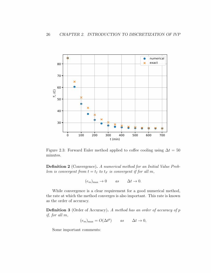
Figure 2.4: Forward Euler method applied to coffee cooling using ∆t = 50and ∆t = 5 minutes. Comparisons to exact solution. Note the difference inscales for the error plots: for ∆t = 50 minutes, the maximum error is about5.5◦ C while for ∆t = 5 minutes, the maximum error is about 0.46◦ C.

RK2 method is given by,

a = ∆tf(vn, tn) (2.7)

b = ∆tf(vn + a/2, tn + ∆t/2) (2.8)

vn+1 = vn + b (2.9)

The final update involves extrapolating the full timestep from vn using b.And, b is evaluated using the estimated slope at tn + ∆t/2.

Note that f is evaluated twice to calculate the new value of vn+1: onceto determine a and once to determine b. So, per iteration, it is essentiallytwice as expensive as Forward Euler (since the cost of evaluating f usuallyis the dominant cost of either Forward Euler or modified Euler).


10 1 100 101

t (min)

10 2

10 1

100

max

erro

r (C)

Figure 2.5: Error convergence for Forward Euler method applied to coffeecooling.

2.4.2 4th order Runge-Kutta Method (RK4)

The most popular form of a fourth-order (p = 4) accurate Runge-Kuttamethod is:

a = ∆tf(vn, tn) (2.10)

b = ∆tf(vn + a/2, tn + ∆t/2) (2.11)

c = ∆tf(vn + b/2, tn + ∆t/2) (2.12)

d = ∆tf(vn + c, tn + ∆t) (2.13)

vn+1 = vn +1

6(a+ 2b+ 2c+ d) (2.14)

Note that this method requires four evaluations of f per iteration.


10 1 100 101

t (min)

10 12

10 10

10 8

10 6

10 4

10 2

100

max

erro

r (C)

FERK2RK4

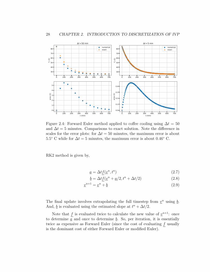
Figure 2.6: Error convergence versus ∆t for Forward Euler, RK2, and RK4methods applied to coffee cooling.

Example 5 (Accuracy and cost of Forward Euler, RK2, and RK4 simulationsof coffee cooling). We now compare convergence and order of accuracy forForward Euler, RK2, and RK4 applied to the coffee cooling problem. Asshown in Figure 2.6, the observed rates are as expected (i.e. p = 1, 2, and4 for Forward Euler, RK2, and RK4) with substantial decreases in the errorfor RK4 compared to Forward Euler and RK2 at the same ∆t. Note that theRK4 result appears to have a decreased rate at the small ∆t values, however,what is actually happening is the machine precision is limiting the error fromdecreasing further.

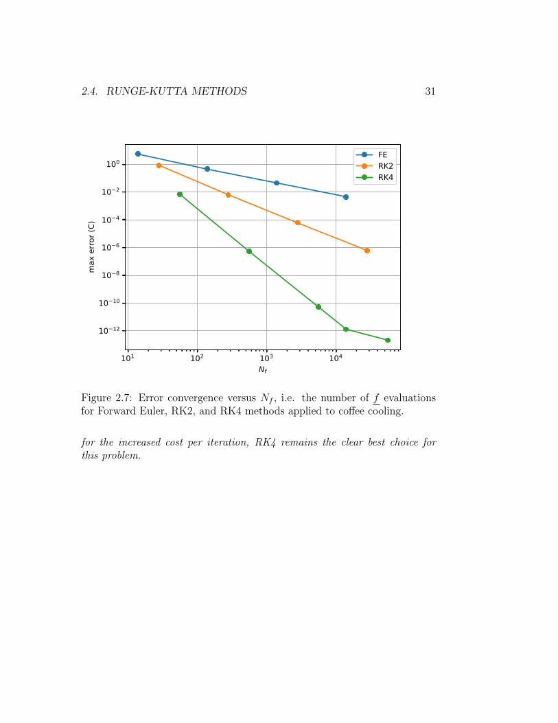
However, for most applications (which will be much more complex thanthis coffee cooling example), the dominant cost is the number of f evaluations.Thus, we should account for the fact that Forward Euler, RK2, ands RK4require 1, 2, and 4 f evaluations per timestep. We can then plot the error asa function of f evaluations. This is shown in Figure 2.7. Even accounting


101 102 103 104

Nf

10 12

10 10

10 8

10 6

10 4

10 2

100

max

erro

r (C)

FERK2RK4

Figure 2.7: Error convergence versus Nf , i.e. the number of f evaluationsfor Forward Euler, RK2, and RK4 methods applied to coffee cooling.

for the increased cost per iteration, RK4 remains the clear best choice forthis problem.

CSE.0002 Introduction to Computational Science and ...

Documents

Transcript of CSE.0002 Introduction to Computational Science and ...