CSE 562 Database Systems Relational Algebra …mpetropo/CSE562-SP10/slides/02AlgebraSQL.pdfCSE 562...

1

CSE 562 Database Systems

Relational Algebra/SQL Overview

UB CSE 562

Some slides are based or modified from originals by Database Systems: The Complete Book,

Pearson Prentice Hall 2nd Edition ©2008 Garcia-Molina, Ullman, and Widom

UB CSE 562 2

Summary

•  Applications’ View of a Relational Database Management System (RDBMS)

•  Relational Algebra Overview •  SQL Overview •  Extended Relational Algebra/Equivalent SQL

UB CSE 562 3

Applications’ View of an RDBMS System

•  Persistent data structure –  Large volume of data –  “Independent” from processes

using the data

•  High-level API for access & modification –  Declarative, automatically optimized

•  Transaction management (ACID) –  Atomicity: all or none happens,

despite failures & errors –  Concurrency –  Isolation: appearance of “one at a time” –  Durability: recovery from failures and other errors

RDBMS Client

Relations, cursors, other…

JDBC/ODBC SQL commands

RDBMS Server

(Web) Application

Relational Database

UB CSE 562 4

Data Structure: Relational Model

•  Relational Databases: Schema + Data

•  Schema: –  collection of tables

(also called relations) –  each table has a set

of attributes –  no repeating relation names,

no repeating attributes in one table

•  Data (also called instance): –  set of tuples –  tuples have one value for each

attribute of the table they belong

Title Director Actor Wild Lynch Winger Sky Berto Winger Reds Beatty Beatty Tango Berto Brando Tango Berto Winger Tango Berto Snyder

Movie

Theater Title Odeon Wild Forum Reds Forum Sky

Schedule

2

UB CSE 562 5

Levels of Abstraction

Disk

Physical Schema

Logical Schema

View View View

describes stored data in terms of data model

includes storage details file organization indexes

UB CSE 562 6

Data Independence

•  Physical Data Independence: Applications are insulated from changes in physical storage details

•  Logical Data Independence: Applications are insulated from changes to logical structure of the data

•  Why are these properties important? – Reduce program maintenance – Logical database design changes over time – Physical database design tuned for

performance

UB CSE 562 7

Programming Interface: JDBC/ODBC

•  How client opens connection with a server •  How access & modification commands are issued

UB CSE 562 8

Access (Query) & Modification Language: SQL

•  SQL –  used by the database user –  declarative: we only describe what we want to

retrieve –  based on tuple relational calculus

•  The input to and the output of a query is always a table (regardless of the query language used)

•  Internal Equivalent of SQL: Relational Algebra –  used internally by the database system –  procedural (operational): we describe how we

retrieve

3

UB CSE 562 9

Summary



UB CSE 562 10

Basic Relational Algebra Operators

•  Selection (σ) –  selects tuples of the

argument relation R that satisfy the condition c

–  The condition c consists of atomic predicates of the form

–  attr = value (attr is an attribute of R)

–  attr1 = attr2

–  other operators possible (e.g. >, <, !=, LIKE)

–  Bigger conditions constructed by conjunctions (AND) and disjunctions (OR) of atomic predicates

Find tuples where director=“Berto”

Find tuples where director=actor

Title Director Actor Sky Berto Winger

Tango Berto Brando Tango Berto Winger Tango Berto Snyder

Title Director Actor Reds Beatty Beatty

Title Director Actor Sky Berto Winger Reds Beatty Beatty Tango Berto Brando Tango Berto Winger Tango Berto Snyder

UB CSE 562 11

Basic Relational Algebra Operators

•  Projection (π) –  returns a table

that has only the attributes attr1, …, attrN of R

–  no duplicate tuples in the result (the example has only one <Tango,Berto> tuple

•  Cartesian Product (x) –  the schema of the result has all

attributes of both R and S –  for every tuple r ∈ R and s ∈ S,

there is a result tuple that consists of r and s

–  if both R and S have an attribute A, then rename to R.A and S.A

Project title & director of Movie

R.A B S.A C 0 1 a b 0 1 c d 2 4 a b 2 4 c d

Title Director Sky Berto

Tango Berto

A B 0 1 2 4

R

A C a b c d

S

R X S

UB CSE 562 12

Basic Relational Algebra Operations

•  Rename (ρ) –  renames attribute A of

relation R into B –  renames relation R into S

•  Union (∪) –  applies to two tables R and S

with same schema –  R ∪ S is the set of tuples that

are in R or S or both

•  Difference (–) –  applies to two tables R and S

with same schema –  R – S is the set of tuples in R

but not in S

Find all people, i.e., actors and directors, of the table Movie

Find all directors who are not actors

4

UB CSE 562 13

Other Relational Algebra Operations

•  Extended Projection: Using the same operator, we allow the list L to contain arbitrary expressions involving attributes:

1.  Arithmetic on attributes, e.g., A+B→C 2.  Duplicate occurrences of the same

attribute •  Example

A B 1 2 3 4

C A1 A2 3 1 1 7 3 3

UB CSE 562 14


•  Theta-Join: R1 ⋈C R2 –  Take the product R1 Χ R2 –  Then apply to the result

•  As for , c can be any boolean-valued condition –  Historic versions of this operator allowed only A θ B,

where θ is =, <, etc.; hence the name “theta-join”

•  Example: Movie ⋈Movie.Title=Schedule.Title Schedule

Movie.Title Director Actor Schedule.Title Theater Wild Lynch Winger Wild Odeon Sky Berto Winger Sky Forum Reds Beatty Beatty Reds Forum

UB CSE 562 15


•  Natural Join: R1 ⋈ R2 A useful join variant connects two relations by: –  Equating attributes of the same name, and –  Projecting out one copy of each pair of equated

attributes

•  Example: Movie ⋈ Schedule

Title Director Actor Theater Wild Lynch Winger Odeon Sky Berto Winger Forum Reds Beatty Beatty Forum

UB CSE 562 16

Building Complex Expressions

•  Algebras allow us to express sequences of operations in a natural way –  Example: in arithmetic – (x + 4)*(y - 3)

•  Relational algebra allows the same •  Three notations, just as in arithmetic:

1.  Sequences of assignment statements 2.  Expressions with several operators 3.  Expression trees

5

UB CSE 562 17

Sequences of Assignments

•  Create temporary relation names •  Renaming can be implied by giving relations a

list of attributes

•  Example: R3 := R1 ⋈C R2 can be written: R4 := R1 X R2 R3 := (R4)

UB CSE 562 18

Expressions in a Single Assignment

•  Example: the theta-join R3 := R1 ⋈C R2 can be written: R3 := (R1 X R2)

•  Precedence of relational operators: 1. Unary operators – select, project, rename – have

highest precedence, bind first 2.  Then come products and joins 3.  Then intersection 4.  Finally, union and set difference bind last

  But you can always insert parentheses to force the order you desire

UB CSE 562 19

Expression Trees

•  Leaves are operands – either variables standing for relations or particular, constant relations

•  Interior nodes are operators, applied to their child or children

UB CSE 562 20

Schemas for Interior Nodes

•  An expression tree defines a schema for the relation associated with each interior node

•  Similarly, a sequence of assignments defines a schema for each relation on the left of the := sign

6

UB CSE 562 21

Schema-Defining Rules 1

•  For union, intersection, and difference, the schemas of the two operands must be the same, so use that schema for the result

•  Selection: schema of the result is the same as the schema of the operand

•  Projection: list of attributes tells us the schema

UB CSE 562 22

Schema-Defining Rules 2

•  Product: the schema is the attributes of both relations –  Use R.A, etc., to distinguish two attributes named A

•  Theta-join: same as product •  Natural join: use attributes of both relations

–  Shared attribute names are merged

•  Renaming: the operator tells the schema

UB CSE 562 23

Relational Algebra on Bags

•  A bag is like a set, but an element may appear more than once –  Multiset is another name for “bag”

•  Example: –  {1,2,1,3} is a bag –  {1,2,3} is also a bag that happens to be a set

•  Bags also resemble lists, but order in a bag is unimportant

•  Example: {1,2,1} = {1,1,2} as bags, but [1,2,1] != [1,1,2] as lists

UB CSE 562 24

Why Bags?

•  SQL, the most important query language for relational databases is actually a bag language –  SQL will eliminate duplicates, but usually only if you

ask it to do so explicitly

•  Some operations, like projection, are much more efficient on bags than sets

7

UB CSE 562 25

Operations on Bags

•  Selection applies to each tuple, so its effect on bags is like its effect on sets

•  Projection also applies to each tuple, but as a bag operator, we do not eliminate duplicates

•  Products and joins are done on each pair of tuples, so duplicates in bags have no effect on how we operate

UB CSE 562 26

Examples

•  Bag Selection

•  Bag Projection

A B 1 2 5 6 1 2

A B 1 2 1 2

A 1 5 1

UB CSE 562 27

Examples

•  Bag Product

•  Bag Theta-Join

A B 1 2 5 6 1 2

A R.B S.B C 1 2 3 4 1 2 7 8 5 6 3 4 5 6 7 8 1 2 3 4 1 2 7 8

B C 3 4 7 8

R ⋈ R.B<S.B S = A R.B S.B C 1 2 3 4 1 2 7 8 5 6 7 8 1 2 3 4 1 2 7 8

UB CSE 562 28

Bag Union

•  Union, intersection, and difference need new definitions for bags

•  An element appears in the union of two bags the sum of the number of times it appears in each bag

•  Example: {1,2,1} ∪ {1,1,2,3,1} = {1,1,1,1,1,2,2,3}

8

UB CSE 562 29

Bag Intersection

•  An element appears in the intersection of two bags the minimum of the number of times it appears in either

•  Example: {1,2,1} ∩ {1,2,3} = {1,2}

UB CSE 562 30

Bag Difference

•  An element appears in the difference A – B of bags as many times as it appears in A, minus the number of times it appears in B –  But never less than 0 times

•  Example: {1,2,1} – {1,2,3} = {1} {1,2,1} – {1,1,1} = {2}

UB CSE 562 31

Beware: Bag Laws != Set Laws

•  Not all algebraic laws that hold for sets also hold for bags

•  Example: the commutative law for union does hold for bags (R ∪ S = S ∪ R) –  Since addition is commutative, adding the number of

times x appears in R and S doesn’t depend on the order of R and S

UB CSE 562 32

An Example of Inequivalence

•  Set union is idempotent, meaning that S ∪ S = S

•  However, for bags, if x appears n times in S, then it appears 2n times in S ∪ S

•  Thus S ∪ S != S in general

9

UB CSE 562 33

Summary



UB CSE 562 34

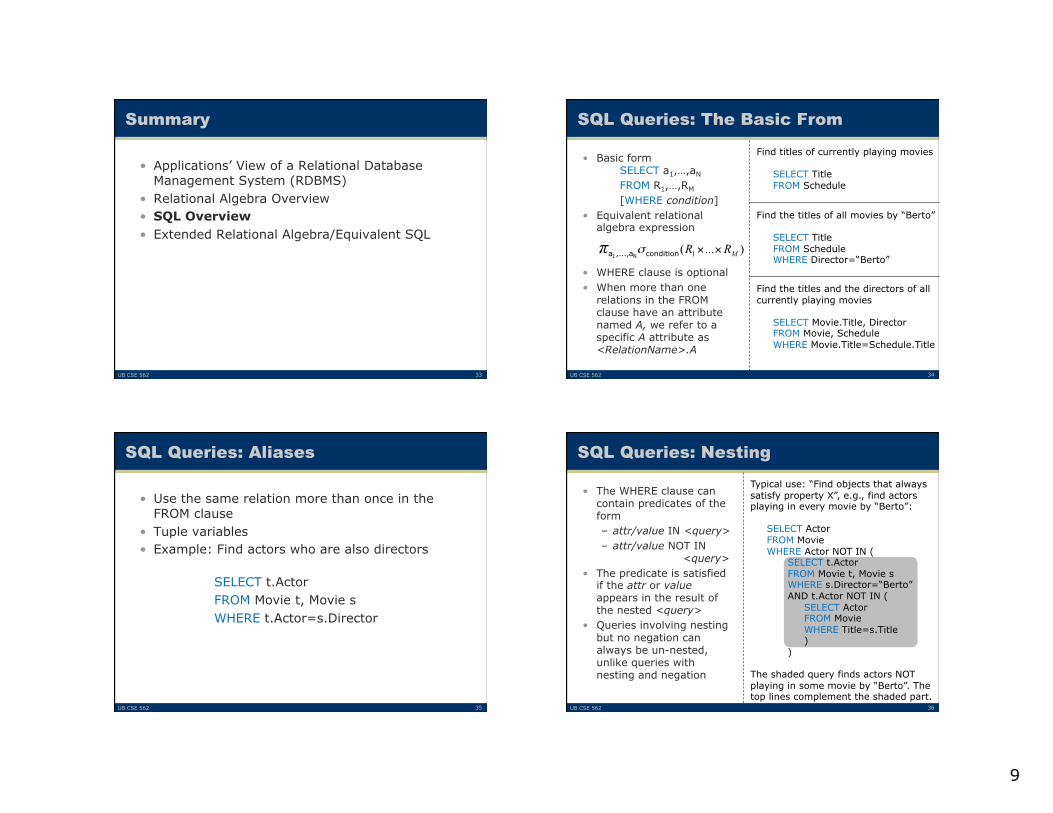
SQL Queries: The Basic From

•  Basic form SELECT a1,…,aN

FROM R1,…,RM

[WHERE condition] •  Equivalent relational

algebra expression

•  WHERE clause is optional •  When more than one

relations in the FROM clause have an attribute named A, we refer to a specific A attribute as <RelationName>.A

Find titles of currently playing movies

SELECT Title FROM Schedule

Find the titles of all movies by “Berto”

SELECT Title FROM Schedule WHERE Director=“Berto”

Find the titles and the directors of all currently playing movies

SELECT Movie.Title, Director FROM Movie, Schedule WHERE Movie.Title=Schedule.Title

UB CSE 562 35

SQL Queries: Aliases

•  Use the same relation more than once in the FROM clause

•  Tuple variables •  Example: Find actors who are also directors

SELECT t.Actor

FROM Movie t, Movie s WHERE t.Actor=s.Director

UB CSE 562 36

SQL Queries: Nesting

•  The WHERE clause can contain predicates of the form –  attr/value IN <query> –  attr/value NOT IN

<query> •  The predicate is satisfied

if the attr or value appears in the result of the nested <query>

•  Queries involving nesting but no negation can always be un-nested, unlike queries with nesting and negation

Typical use: “Find objects that always satisfy property X”, e.g., find actors playing in every movie by “Berto”:

SELECT Actor FROM Movie WHERE Actor NOT IN (

SELECT t.Actor FROM Movie t, Movie s WHERE s.Director=“Berto” AND t.Actor NOT IN ( SELECT Actor FROM Movie WHERE Title=s.Title ) )

The shaded query finds actors NOT playing in some movie by “Berto”. The top lines complement the shaded part.

10

UB CSE 562 37

Homework Problem

•  Compare with shaded sub-query of previous slide. The sample data may help you.

SELECT Actor FROM Movie WHERE Actor NOT IN ( SELECT Actor FROM Movie WHERE Director=“Berto” )

Actor Director Movie

a B 1

a B 2

b B 1

c X 3

d B 1

d B 2

d X 3

UB CSE 562 38

Nested Queries: Existential Quantification

•  A op ANY <nested query> is satisfied if there is a value X in the result of the <nested query> and the condition A op X is satisfied –  (= ANY) ≡ IN –  But, (≠ ANY) ≡ NOT IN

Find directors of currently playing movies

SELECT Director FROM Movie WHERE Title = ANY

SELECT Title FROM Schedule

UB CSE 562 39

Nested Queries: Universal Quantification

•  A op ALL <nested query> is satisfied if for every value X in the result of the <nested query> the condition A op X is satisfied –  (≠ ALL) ≡ NOT IN –  But, (= ALL) ≡ IN

Find the employees with the highest salary

SELECT Name FROM Employee WHERE Salary >= ALL

SELECT Salary FROM Employee

UB CSE 562 40

Nested Queries: Set Comparison

<nested query 1> CONTAINS

<nested query 2>

Find actors playing in every movie by “Berto”

SELECT s.Actor FROM Movie s WHERE

(SELECT Title FROM Movie t WHERE t.Actor = s.Actor) CONTAINS (SELECT Title FROM Movie WHERE Director = “Berto”)

11

UB CSE 562 41

SQL: Union, Intersection, Difference

•  Union <SQL query 1>

UNION <SQL query 2>

•  Intersection <SQL query 1>

INTERSECT <SQL query 2>

•  Difference <SQL query 1>

MINUS <SQL query 2>

Find all actors or directors

(SELECT Actor FROM Movie) UNION (SELECT Director FROM Movie)

Find all actors who are not directors

(SELECT Actor FROM Movie) MINUS (SELECT Director FROM Movie)

UB CSE 562 42

NULL Values

•  Tuples in SQL relations can have NULL as a value for one or more components

•  Meaning depends on context. Two common cases: –  Missing value: e.g., we know movie Tango has a third

actor, but we don’t know who she/he is

–  Inapplicable: e.g., the value of attribute spouse for an unmarried person

Title Director Actor Tango Berto Brando Tango Berto Winger Tango Berto NULL

UB CSE 562 43

Comparing NULL’s to Values

•  The logic of conditions in SQL is really 3-valued logic: TRUE, FALSE, UNKNOWN

•  Comparing any value (including NULL itself) with NULL yields UNKNOWN

•  A tuple is in a query answer iff the WHERE clause is TRUE (not FALSE or UNKNOWN)

UB CSE 562 44

Three-Valued Logic

•  To understand how AND, OR, and NOT work in 3-valued logic, think of TRUE = 1, FALSE = 0, and UNKNOWN = ½

•  AND = MIN; OR = MAX, NOT(x) = 1-x •  Example:

TRUE AND (FALSE OR NOT(UNKNOWN)) = MIN(1, MAX(0, (1 - ½ ))) = MIN(1, MAX(0, ½ )) = MIN(1, ½ ) = ½

12

UB CSE 562 45

Surprising Example

•  From the following Sells relation:

SELECT book FROM Sells WHERE price < 20.00 OR price >= 20.00;

UNKNOWN UNKNOWN

UNKNOWN

book store price Harry Potter Amazon NULL

UB CSE 562 46

Reason: 2-Valued Laws != 3-Valued Laws

•  Some common laws, like commutativity of AND, hold in 3-valued logic

•  But not others, e.g., the law of the excluded middle: p OR NOT p = TRUE –  When p = UNKNOWN, the left side is

MAX( ½, (1 – ½ )) = ½ != 1

UB CSE 562 47

Bag Semantics

•  Although the SELECT-FROM-WHERE statement uses bag semantics, the default for union, intersection, and difference is set semantics –  That is, duplicates are eliminated as the operation is

applied

UB CSE 562 48

Motivation: Efficiency

•  When doing projection, it is easier to avoid eliminating duplicates –  Just work tuple-at-a-time

•  For intersection or difference, it is most efficient to sort the relations first –  At that point you may as well eliminate the duplicates

anyway

13

UB CSE 562 49

Controlling Duplicate Elimination

•  Force the result to be a set by SELECT DISTINCT …

•  Force the result to be a bag (i.e., don’t eliminate duplicates) by ALL, as in

… UNION ALL …

UB CSE 562 50

Summary



UB CSE 562 51

The Extended Algebra

δ = eliminate duplicates from bags

τ = sort tuples

γ = grouping and aggregation

UB CSE 562 52

Duplicate Elimination

•  R1 := δ(R2)

•  R1 consists of one copy of each tuple that appears in R2 one or more times

•  Example: R =

δ(R)=

A B 1 2 3 4 1 2

A B 1 2 3 4

14

UB CSE 562 53

Sorting

•  R1 := τL (R2) –  L is a list of some of the attributes of R2

•  R1 is the list of tuples of R2 sorted first on the value of the first attribute on L, then on the second attribute of L, and so on –  Break ties arbitrarily

•  τ is the only operator whose result is neither a set nor a bag

UB CSE 562 54

Aggregation Operators

•  Aggregation operators are not operators of relational algebra

•  Rather, they apply to entire columns of a table and produce a single result

•  The most important examples: SUM, AVG, COUNT, MIN, and MAX

•  Example: R =

SUM(A) = 7 COUNT(A) = 3 MAX(B) = 4 AVG(B) = 3

A B 1 3 3 4 3 2

UB CSE 562 55

Grouping Operator

•  R1 := γL (R2) L is a list of elements that are either: 1.  Individual (grouping) attributes 2.  AGG(A), where AGG is one of the aggregation

operators and A is an attribute –  An arrow and a new attribute name renames the component

UB CSE 562 56

Applying γL(R)

•  Group R according to all the grouping attributes on list L –  That is: form one group for each distinct list of values

for those attributes in R

•  Within each group, compute AGG(A) for each aggregation on list L

•  Result has one tuple for each group: 1.  The grouping attributes and 2.  Their group’s aggregations

15

UB CSE 562 57

First, group R by A and B:

Then, average C within groups:

Example: Grouping/Aggregation

R =

γA,B,AVG(C)->X (R) = ??

A B C 1 2 3 4 5 6 1 2 5

A B C 1 2 3 1 2 5 4 5 6

A B X 1 2 4 4 5 6

UB CSE 562 58

Outerjoin

•  Suppose we join R ⋈C S

•  A tuple of R that has no tuple of S with which it joins is said to be dangling –  Similarly for a tuple of S

•  Outerjoin preserves dangling tuples by padding them with NULLs

UB CSE 562 59

Example: Outerjoin

R = A B 1 2 4 5

S = B C 2 3 6 7

(1,2) joins with (2,3), but the other two tuples are dangling

R OUTERJOIN S = A B C 1 2 3 4 5 NULL

NULL 6 7

UB CSE 562 60

SQL Outerjoins

•  R OUTER JOIN S is the core of an outerjoin expression

•  It is modified by: 1. Optional NATURAL in front of OUTER 2. Optional ON <condition> after JOIN 3. Optional LEFT, RIGHT, or FULL before OUTER

  LEFT = pad dangling tuples of R only   RIGHT = pad dangling tuples of S only   FULL = pad both; this choice is the default

Only one of these

16

UB CSE 562 61

SQL Aggregations

•  SUM, AVG, COUNT, MIN, and MAX can be applied to a column in a SELECT clause to produce that aggregation on the column

•  Also, COUNT(*) counts the number of tuples •  Example: Find the average salary of all employees

Name Dept Salary Joe Toys 45 Nick PCs 50 Jim Toys 35 Jack PCs 40

Employee SELECT AvgSal = AVG(Salary) FROM Employee

AvgSal 42.5

UB CSE 562 62

Eliminating Duplicates in a SQL Aggregation

•  Use DISTINCT inside an aggregation •  Example: Find the number of different departments:

SELECT COUNT(DISTINCT Dept) FROM Employee


Employee

UB CSE 562 63

NULL’s Ignored in SQL Aggregation

•  NULL never contributes to a sum, average, or count, and can never be the minimum or maximum of a column

•  But if there are no non-NULL values in a column, then the result of the aggregation is NULL –  Exception: COUNT of an empty set is 0

UB CSE 562 64

Example: Effect of NULL’s

SELECT COUNT(*) FROM Employee WHERE Dept=“Toys”;

SELECT COUNT(Salary) FROM Employee WHERE Dept=“Toys”;

The number of employees in the Toys department

The number of employees in the Toys department

with a known salary

Name Dept Salary Joe Toys 45 Jim Toys NULL Jack PCs 40

Employee

17

UB CSE 562 65

SQL Grouping

•  We may follow a SELECT-FROM-WHERE expression by GROUP BY and a list of attributes

•  The relation that results from the SELECT-FROM-WHERE is grouped according to the values of all those attributes, and any aggregation is applied only within each group

UB CSE 562 66

Example: SQL Grouping

Find the average salary for each department:

SELECT Dept, AvgSal = AVG(Salary) FROM Employee GROUP BY Dept


Employee

Dept AvgSal Toys 40 PCs 45

UB CSE 562 67

Example: Null Values and Aggregates

•  Example:

•  select count(a), count(b), avg(b), count(*) from R group by a

a b x 1 x 2 x null

null null null null

R

count(a) count(b) avg(b) count(*) 3 2 1.5 3 0 0 null 2

UB CSE 562 68

Restriction on SELECT Lists With Aggregation

•  If any aggregation is used, then each element of the SELECT list must be either: 1.  Aggregated, or 2.  An attribute on the GROUP BY list

•  Example: You might think you could find the department with the highest salary by: SELECT Dept, MaxSal = MAX(Salary) FROM Employee But this query is illegal in SQL

18

UB CSE 562 69

SQL HAVING Clauses

•  HAVING <condition> may follow a GROUP BY clause

•  If so, the condition applies to each group, and groups not satisfying the condition are eliminated

UB CSE 562 70

Example: SQL HAVING

•  Example: Find the average salary of for each department that has either more than 1 employee or starts with a “To”:

SELECT Dept, AvgSal=(AVG(Salary)) FROM Employee GROUP BY Dept HAVING COUNT(Name) > 1 OR Dept LIKE “To”

UB CSE 562 71

Requirements on HAVING Conditions

•  Conditions may refer to attributes only if they are either: 1.  A grouping attribute, or 2.  Aggregated

(same condition as for SELECT clauses with aggregation)

UB CSE 562 72

Summary of SQL Queries

•  A query in SQL can consist of up to six clauses, but only the first two, SELECT and FROM, are mandatory.

•  The clauses are specified in the following order:

SELECT <attribute list> FROM <table list> [WHERE <condition>] [GROUP BY <grouping attribute(s)>] [HAVING <group condition>] [ORDER BY <attribute list>]

19

UB CSE 562 73

Summary of SQL Queries (cont’d)

•  The SELECT-clause lists the attributes or functions to be retrieved

•  The FROM-clause specifies all relations (or aliases) needed in the query but not those needed in nested queries

•  The WHERE-clause specifies the conditions for selection and join of tuples from the relations specified in the FROM-clause

•  GROUP BY specifies grouping attributes •  HAVING specifies a condition for selection of groups •  ORDER BY specifies an order for displaying the result of a

query •  A query is evaluated by first applying the WHERE-clause,

then GROUP BY and HAVING, and finally the SELECT-clause

UB CSE 562 74

Recursion in SQL

•  SQL:1999 permits recursive queries •  Example: find all employee-manager pairs, where the employee

reports to the manager directly or indirectly (that is manager’s manager, manager’s manager’s manager, etc.)

WITH RECURSIVE empl(employee_name, manager_name) AS ( SELECT employee_name, manager_name FROM manager UNION SELECT manager.employee_name, empl.manager_name FROM manager, empl WHERE manager.manager_name = empl.employe_name) SELECT * FROM empl

•  This example query computes the transitive closure of the manager relation

UB CSE 562 75

The Power of Recursion

•  Recursive queries make it possible to write queries, such as transitive closure queries, that cannot be written without recursion or iteration –  Intuition: Without recursion, a non-recursive non-

iterative program can perform only a fixed number of joins of manager with itself – This can give only a fixed number of levels of

managers – Given a program we can construct a database with

a greater number of levels of managers on which the program will not work

UB CSE 562 76

The Power of Recursion (cont’d)

•  Computing transitive closure –  The next slide shows a manager relation and finds all

employees managed by “Jones” –  Each step of the iterative process constructs an

extended version of empl from its recursive definition –  The final result is called the fixed point of the recursive

definition

20

UB CSE 562 77

Example of Fixed-Point Computation

UB CSE 562 78

The Power of Recursion (cont’d)

•  Recursive queries are required to be monotonic, that is, if we add tuples to manager the query result contains all of the tuples it contained before, plus possibly more

•  Example: SELECT AvgSal = AVG(Salary) FROM Employee is not monotone in Employee

–  Inserting a tuple into Employee usually changes the average salary and thus deletes the old average salary

UB CSE 562 79

SQL as a Data Manipulation Language: Insertions

Inserting tuples INSERT INTO R

VALUES (v1,…,vk); •  some values may be left

NULL •  use results of queries for

insertion INSERT INTO R SELECT …

FROM … WHERE …

INSERT INTO Movie VALUES (“Brave”, “Gibson”, “Gibson”);

INSERT INTO Movie(Title,Director) VALUES (“Brave”, “Gibson”);

INSERT INTO EuroMovie SELECT * FROM Movie WHERE Director = “Berto”

UB CSE 562 80

SQL as a Data Manipulation Language: Deletions

•  Deletion basic form: delete every tuple that satisfies <cond> DELETE FROM R WHERE <cond>

•  Delete the movies that are not currently playing DELETE FROM Movie WHERE Title NOT IN SELECT Title FROM Schedule

21

UB CSE 562 81

SQL as a Data Manipulation Language: Updates

•  Update basic form: update every tuple that satisfies <cond> in the way specified by the SET clause UPDATE R SET A1=<exp1>,…,Ak=<expk> WHERE <cond>

•  Change all “Berto” entries to “Bertoluci” UPDATE Movie SET Director=“Bertoluci” WHERE Director=“Berto”

•  Increase all salaries in the Toys dept by 10% UPDATE Employee SET Salary = 1.1 * Salary WHERE Dept = “Toys”

•  The “rich get richer” exercise: Increase by 10% the salary of the employee with the highest salary

UB CSE 562 82

This Time

•  Relational Algebra –  Chapter 2: 2.4 –  Chapter 5: 5.1, 5.2

•  SQL –  Chapter 6 –  Chapter 10: 10.2

CSE 562 Database Systems Relational Algebra …mpetropo/CSE562-SP10/slides/02AlgebraSQL.pdfCSE 562...

Documents

Transcript of CSE 562 Database Systems Relational Algebra …mpetropo/CSE562-SP10/slides/02AlgebraSQL.pdfCSE 562...