CSE-473 Artificial Intelligence

Partially-Observable MDPS(POMDPs)

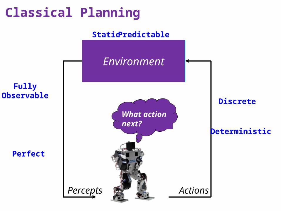
Classical Planning

What action next?

Percepts Actions

Environment

Static

Fully Observable

Perfect

Predictable

Discrete

Deterministic

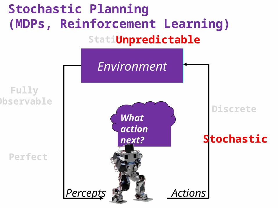
Stochastic Planning (MDPs, Reinforcement Learning)

What action next?

Percepts Actions

Environment

Static

Fully Observable

Perfect

Stochastic

Unpredictable

Discrete

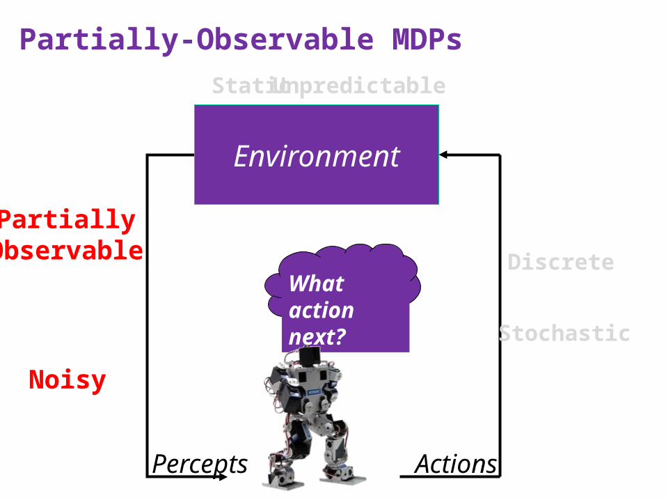
Partially-Observable MDPs

What action next?

Percepts Actions

Environment

Static

Partially Observable

Noisy

Stochastic

Unpredictable

Discrete

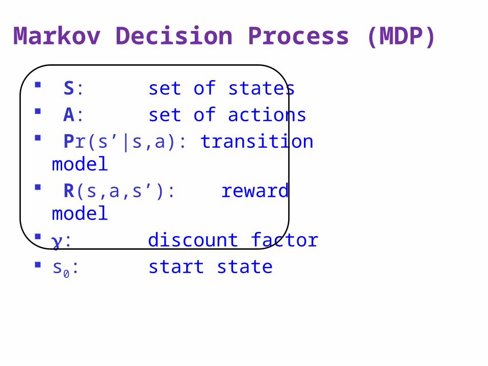
Markov Decision Process (MDP)

S: set of states A: set of actions Pr(s’|s,a): transition model R(s,a,s’): reward model : discount factor s0: start state

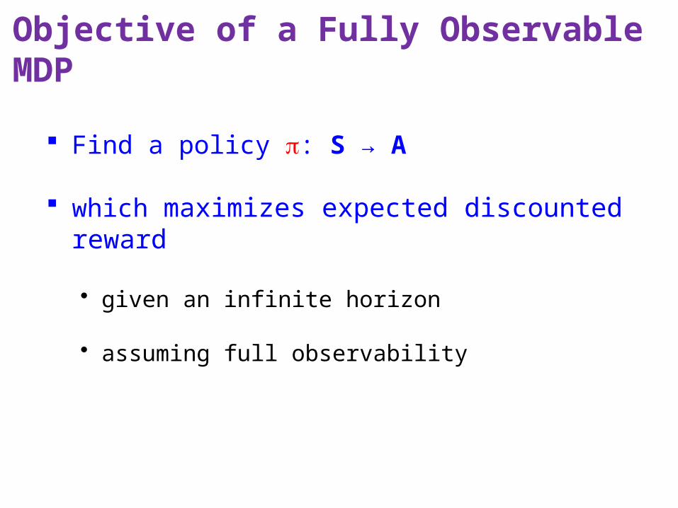
Objective of a Fully Observable MDP

Find a policy : S → A

which maximizes expected discounted reward

• given an infinite horizon

• assuming full observability

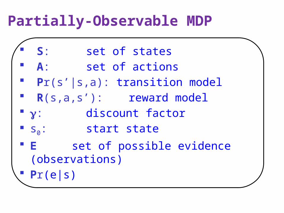
Partially-Observable MDP

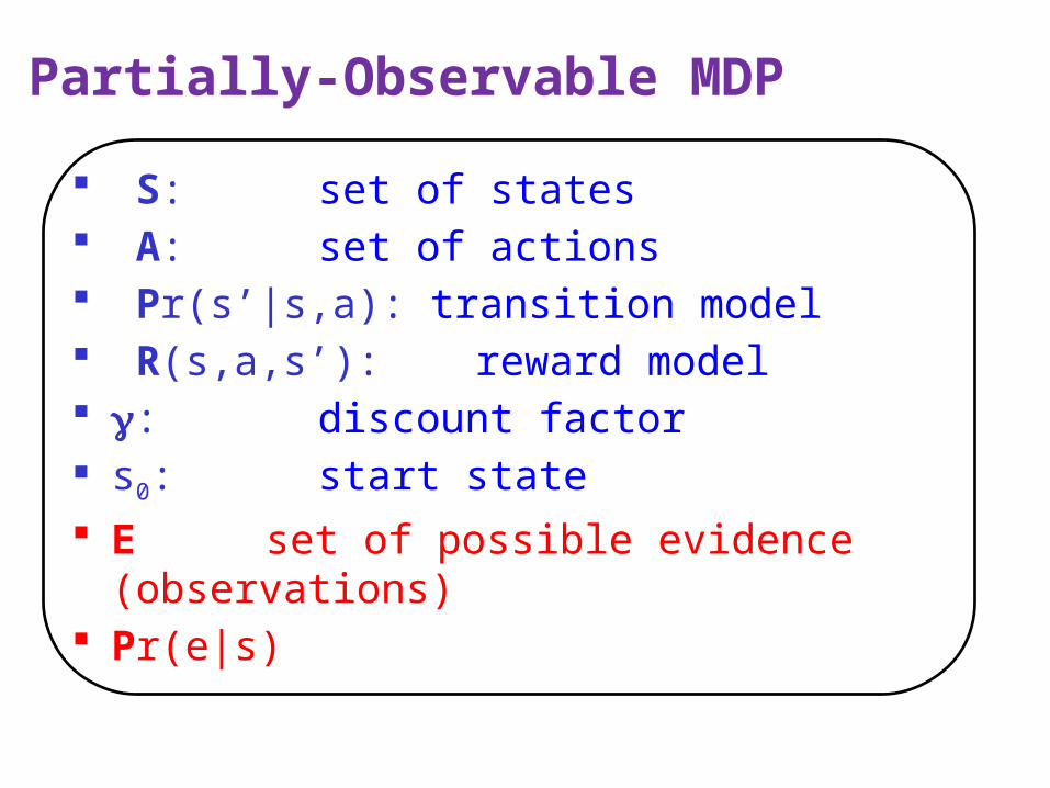
S: set of states A: set of actions Pr(s’|s,a): transition model R(s,a,s’): reward model : discount factor s0: start state E set of possible evidence (observations) Pr(e|s)

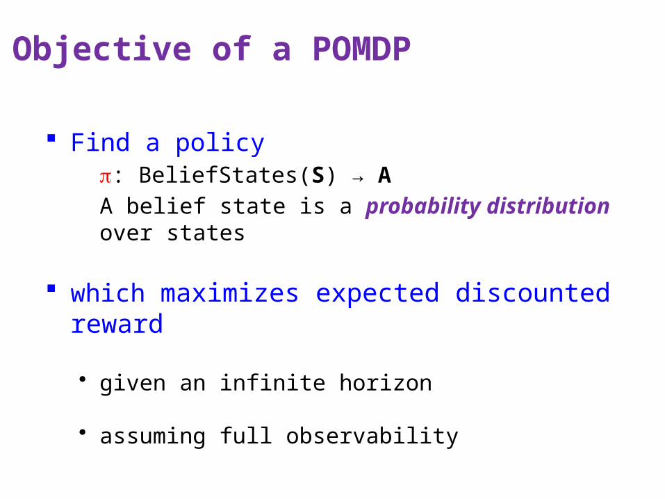
Objective of a POMDP

Find a policy : BeliefStates(S) → A A belief state is a probability distribution over states

which maximizes expected discounted reward

• given an infinite horizon

• assuming full observability

9

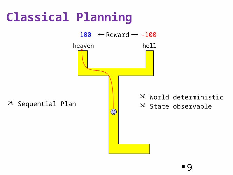
Classical Planning

hellheaven

• World deterministic• State observable• Sequential Plan

Reward100 -100

10

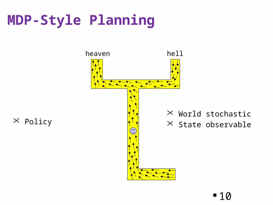
MDP-Style Planning

hellheaven

• World stochastic• State observable• Policy

11

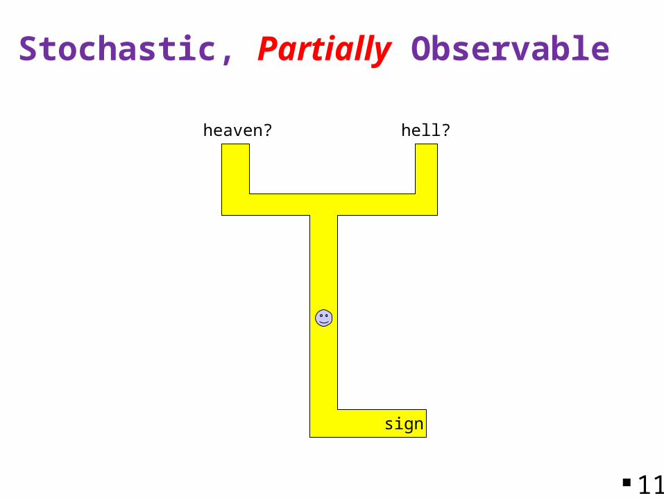
Stochastic, Partially Observable

sign

hell?heaven?

12

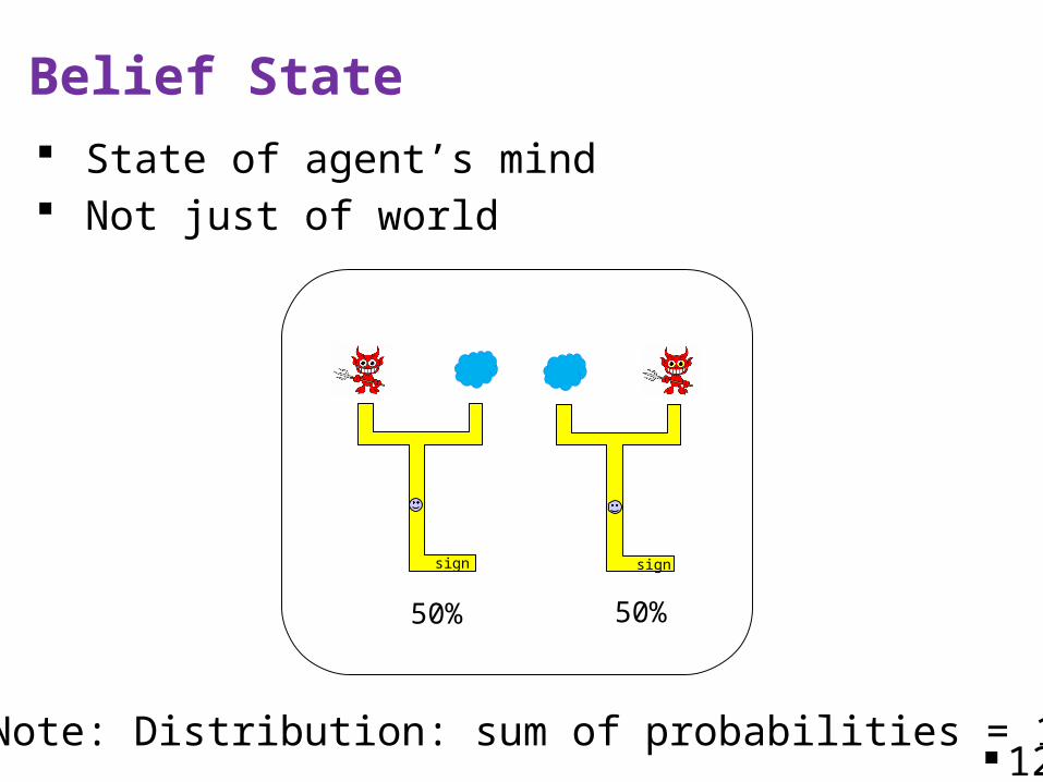
Belief State

sign sign

50% 50%

State of agent’s mind Not just of world

Note: Distribution: sum of probabilities = 1

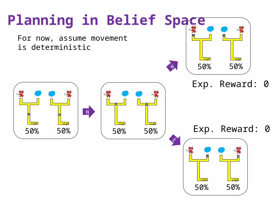
Planning in Belief Space

sign sign

50% 50%sign sign

50% 50%

sign sign

50% 50%

sign sign

50% 50%

N

W

E

Exp. Reward: 0

Exp. Reward: 0

For now, assume movement is deterministic

Partially-Observable MDP

S: set of states A: set of actions Pr(s’|s,a): transition model R(s,a,s’): reward model : discount factor s0: start state E set of possible evidence (observations) Pr(e|s)

Evidence Model

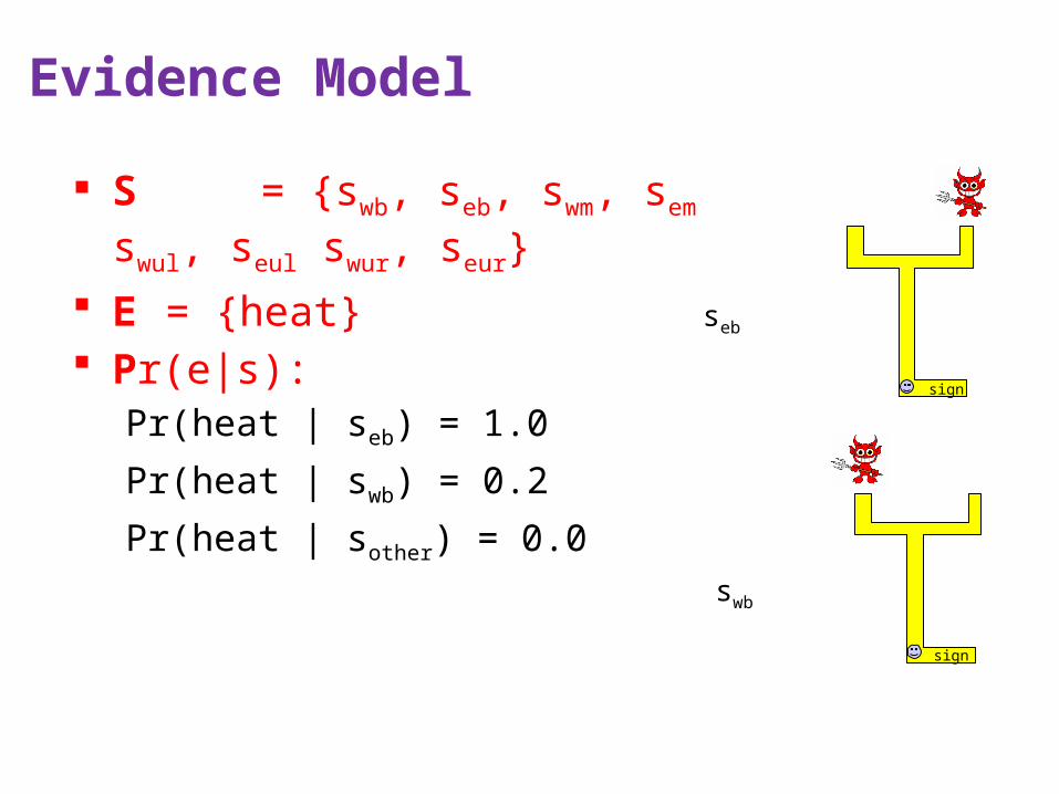
S = {swb, seb, swm, sem swul, seul swur, seur} E = {heat} Pr(e|s):

Pr(heat | seb) = 1.0

Pr(heat | swb) = 0.2

Pr(heat | sother) = 0.0

sign

sign

seb

swb

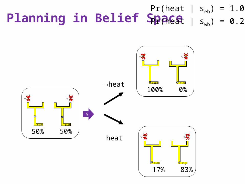
Planning in Belief Space

sign sign

50% 50%

sign sign

100% 0%

S

sign sign

17% 83%

heat

heat

Pr(heat | seb) = 1.0

Pr(heat | swb) = 0.2

17

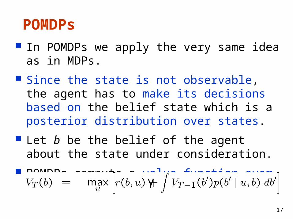
POMDPs In POMDPs we apply the very same idea as in MDPs. Since the state is not observable, the agent has to make

its decisions based on the belief state which is a posterior distribution over states.

Let b be the belief of the agent about the state under consideration.

POMDPs compute a value function over belief space:

γ

18

Problems

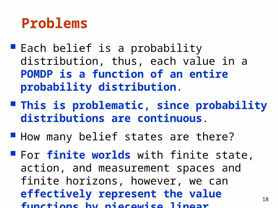
Each belief is a probability distribution, thus, each value in a POMDP is a function of an entire probability distribution.

This is problematic, since probability distributions are continuous.

How many belief states are there? For finite worlds with finite state, action, and

measurement spaces and finite horizons, however, we can effectively represent the value functions by piecewise linear functions.

19

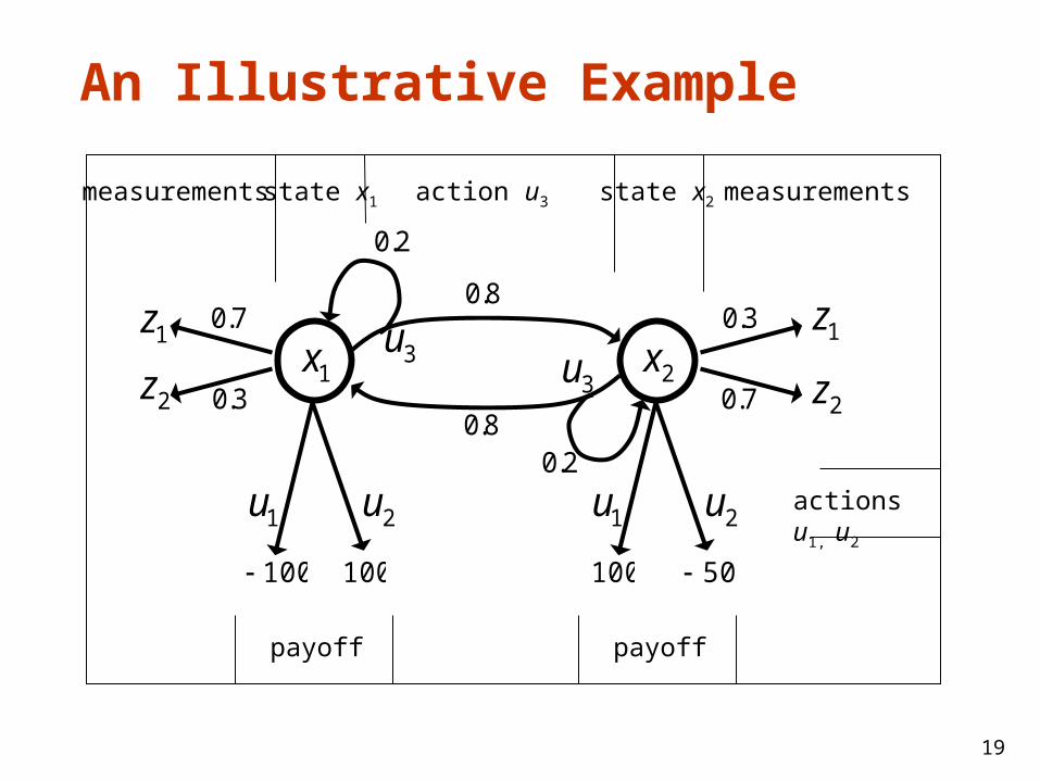
An Illustrative Example

2x1x 3u8.0

2z1z

3u

2.0

8.02.0

7.0

3.0

3.0

7.0

measurements action u3 state x2

payoff

measurements

1u 2u 1u 2u

100 50100 100

actions u1, u2

payoff

state x1

1z

2z

20

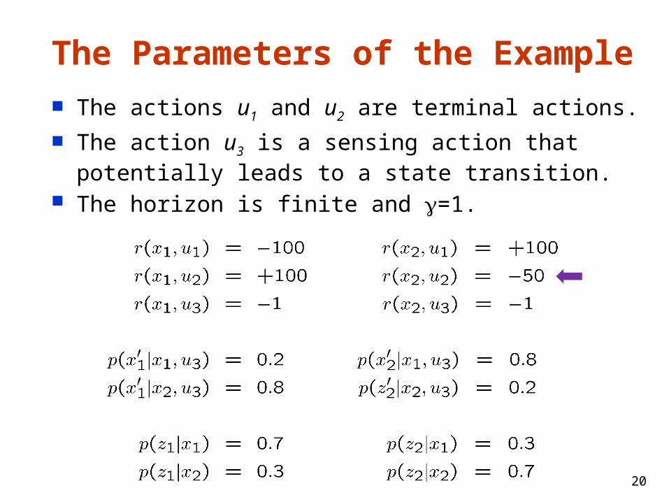
The Parameters of the Example The actions u1 and u2 are terminal actions. The action u3 is a sensing action that potentially

leads to a state transition. The horizon is finite and =1.

21

Payoff in POMDPs

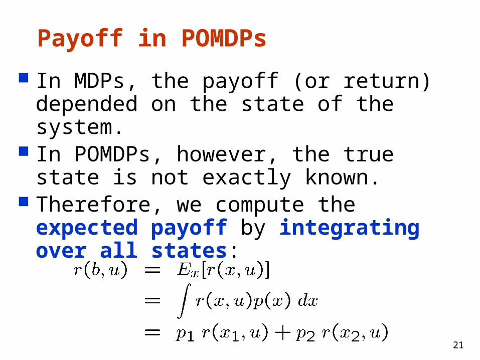
In MDPs, the payoff (or return) depended on the state of the system.

In POMDPs, however, the true state is not exactly known.

Therefore, we compute the expected payoff by integrating over all states:

22

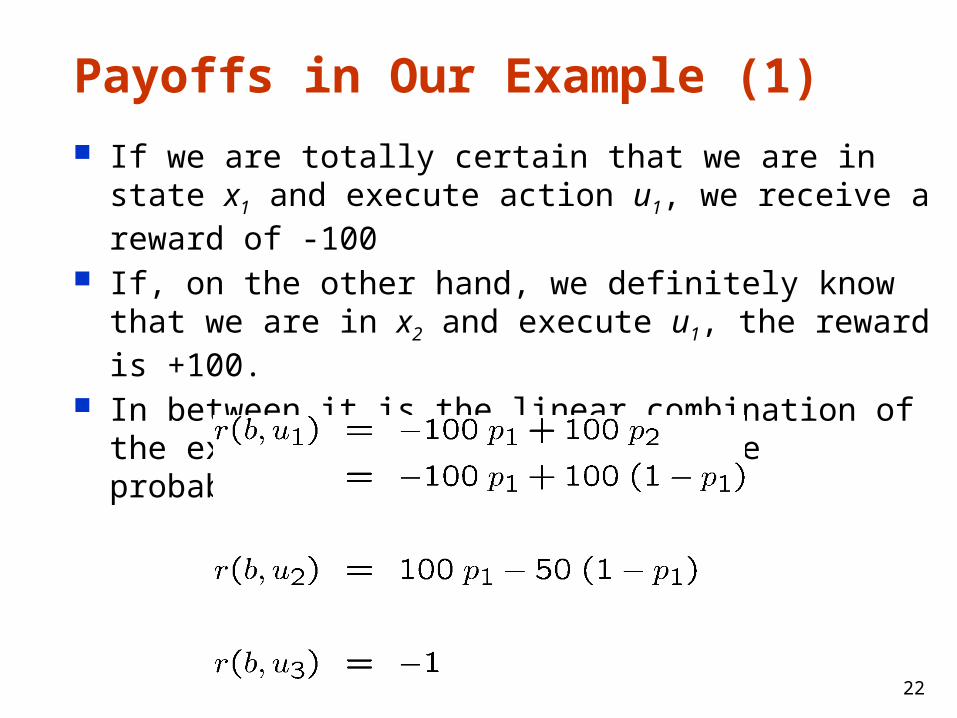
Payoffs in Our Example (1)

If we are totally certain that we are in state x1 and execute action u1, we receive a reward of -100

If, on the other hand, we definitely know that we are in x2 and execute u1, the reward is +100.

In between it is the linear combination of the extreme values weighted by the probabilities

23

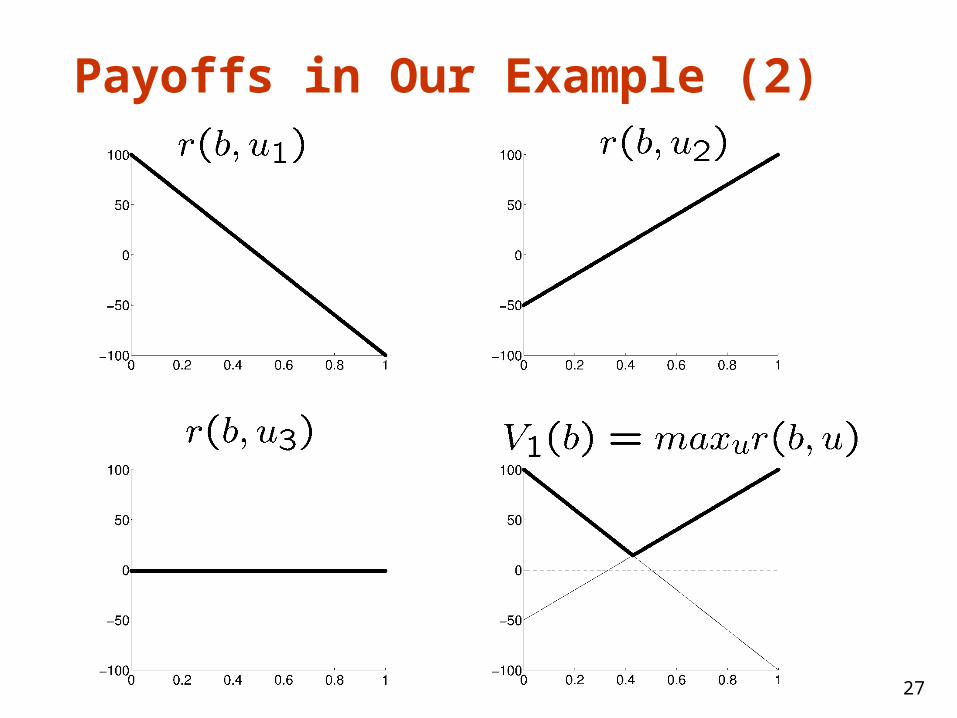
Payoffs in Our Example (2)

24

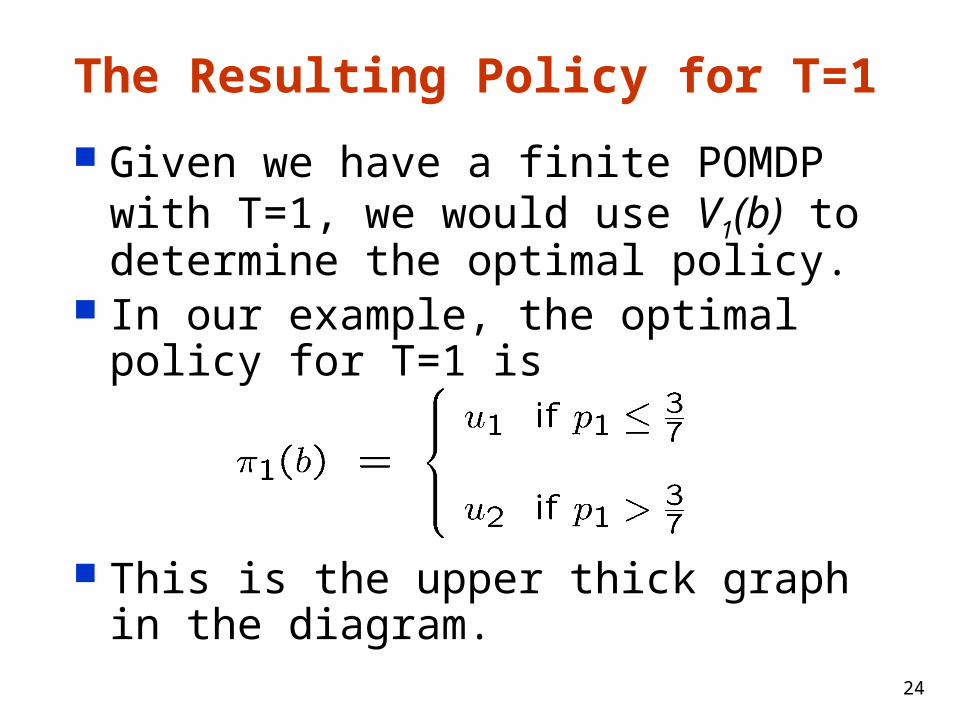
The Resulting Policy for T=1

Given we have a finite POMDP with T=1, we would use V1(b) to determine the optimal policy.

In our example, the optimal policy for T=1 is

This is the upper thick graph in the diagram.

25

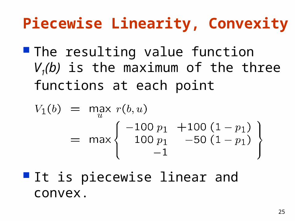
Piecewise Linearity, Convexity

The resulting value function V1(b) is the maximum of the three functions at each point

It is piecewise linear and convex.

26

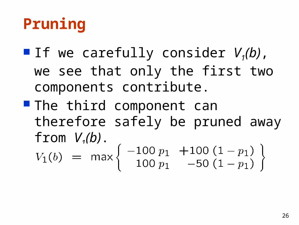
Pruning

If we carefully consider V1(b), we see that only the first two components contribute.

The third component can therefore safely be pruned away from V1(b).

27

Payoffs in Our Example (2)

28

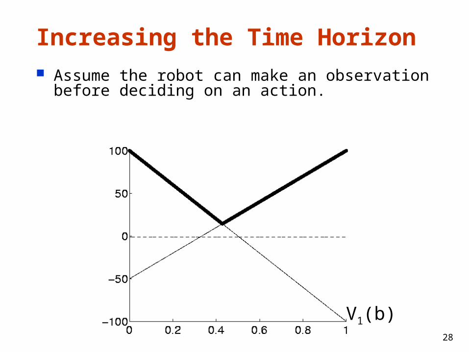
Increasing the Time Horizon Assume the robot can make an observation before

deciding on an action.

V1(b)

29

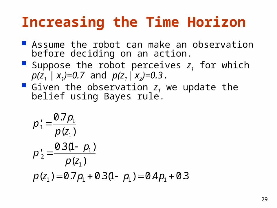
Increasing the Time Horizon Assume the robot can make an observation before

deciding on an action. Suppose the robot perceives z1 for which

p(z1 | x1)=0.7 and p(z1| x2)=0.3. Given the observation z1 we update the belief using

Bayes rule.

3.04.0)1(3.07.0)(

)(

)1(3.0'

)(

7.0'

1111

1

12

1

11

pppzp

zp

pp

zp

pp

30

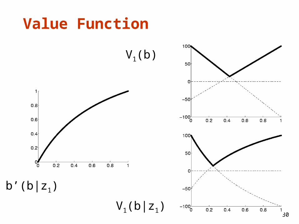
Value Function

b’(b|z1)

V1(b)

V1(b|z1)

31

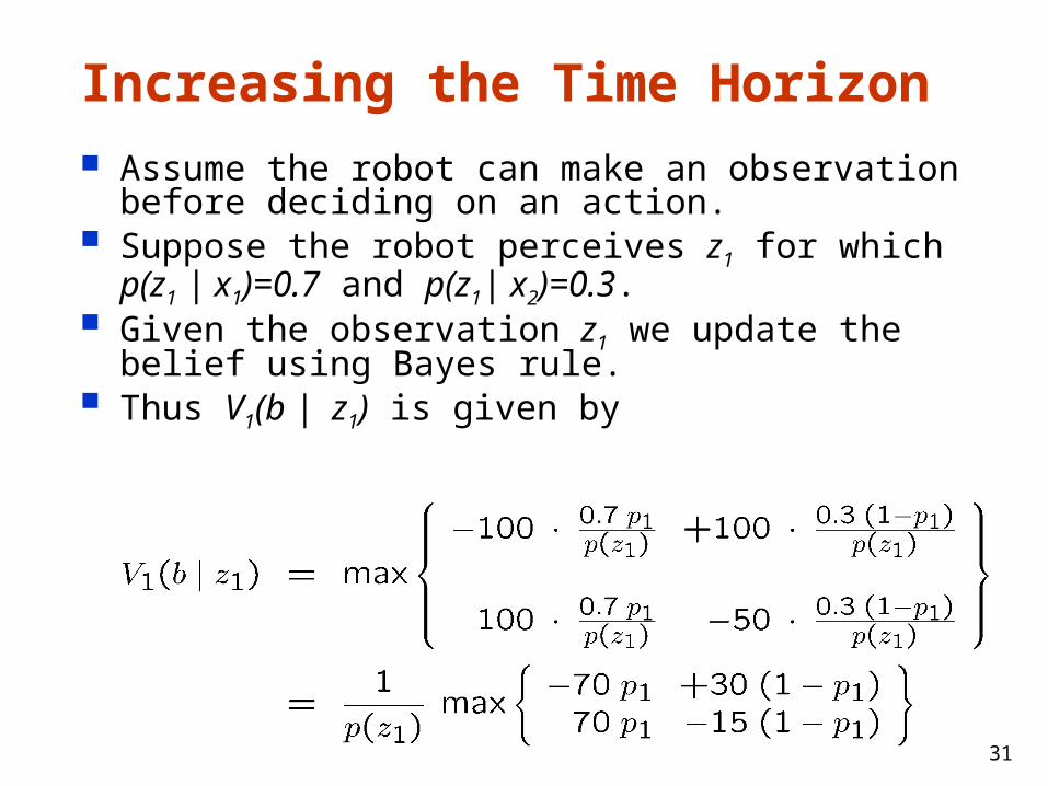
Increasing the Time Horizon Assume the robot can make an observation before

deciding on an action. Suppose the robot perceives z1 for which

p(z1 | x1)=0.7 and p(z1| x2)=0.3. Given the observation z1 we update the belief using

Bayes rule. Thus V1(b | z1) is given by

32

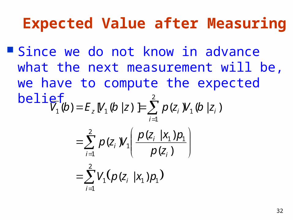
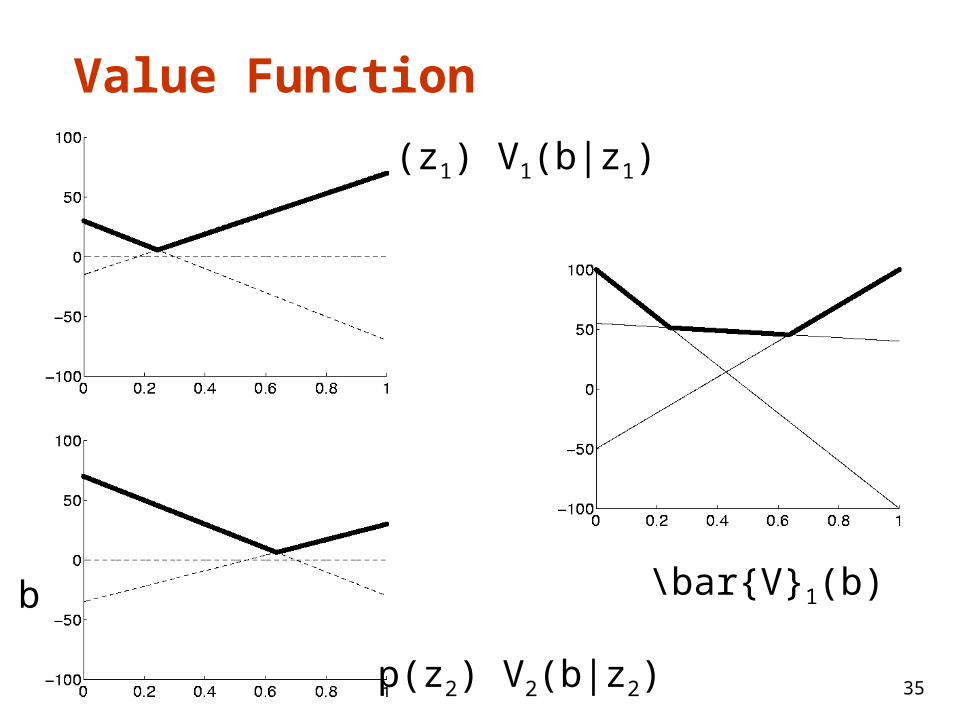
Expected Value after Measuring

Since we do not know in advance what the next measurement will be, we have to compute the expected belief

2

1111

2

1

111

2

1111

)|(

)(

)|()(

)|()()]|([)(

ii

i i

ii

iiiz

pxzpV

zp

pxzpVzp

zbVzpzbVEbV

33

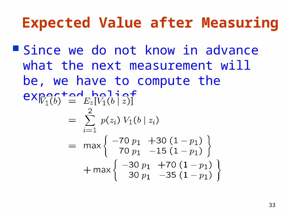
Expected Value after Measuring

Since we do not know in advance what the next measurement will be, we have to compute the expected belief

34

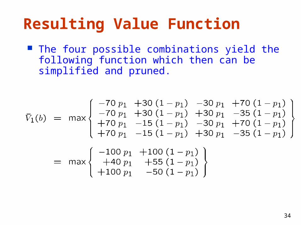
Resulting Value Function The four possible combinations yield the

following function which then can be simplified and pruned.

35

Value Function

b’(b|z1)

p(z1) V1(b|z1)

p(z2) V2(b|z2)

\bar{V}1(b)

36

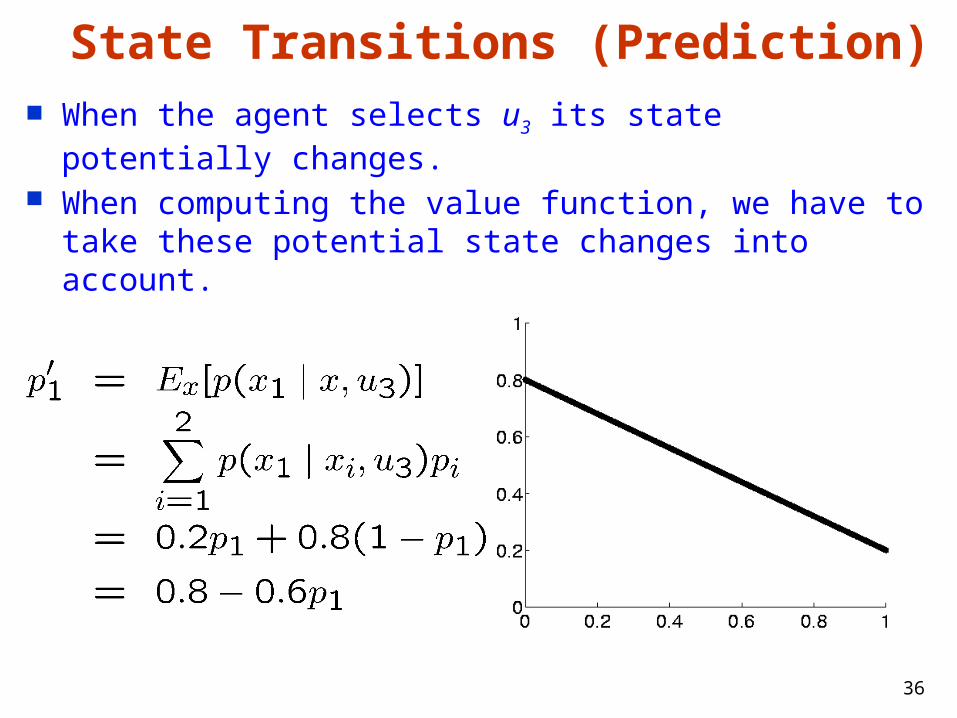
State Transitions (Prediction) When the agent selects u3 its state potentially

changes. When computing the value function, we have to take

these potential state changes into account.

37

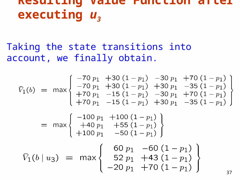
Resulting Value Function after executing u3

Taking the state transitions into account, we finally obtain.

38

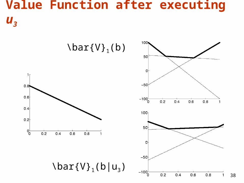
Value Function after executing u3

\bar{V}1(b)

\bar{V}1(b|u3)

39

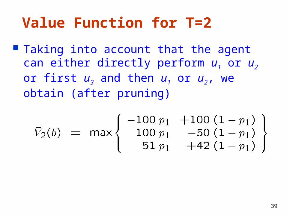
Value Function for T=2

Taking into account that the agent can either directly perform u1 or u2 or first u3 and then u1 or u2, we obtain (after pruning)

40

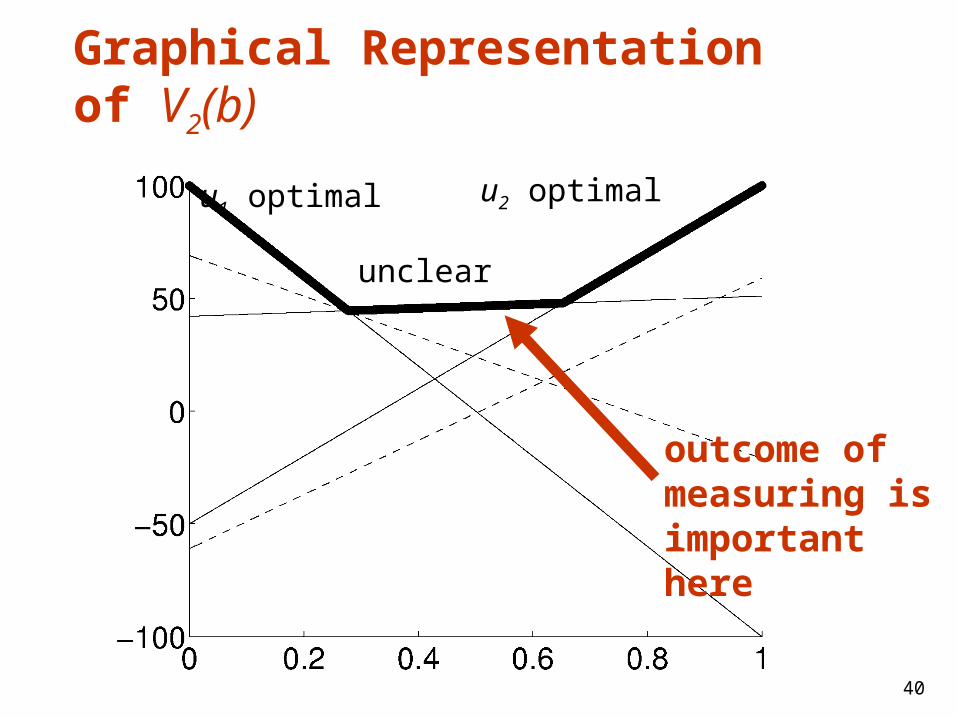
Graphical Representation of V2(b)

u1 optimal u2 optimal

unclear

outcome of measuring is important here

41

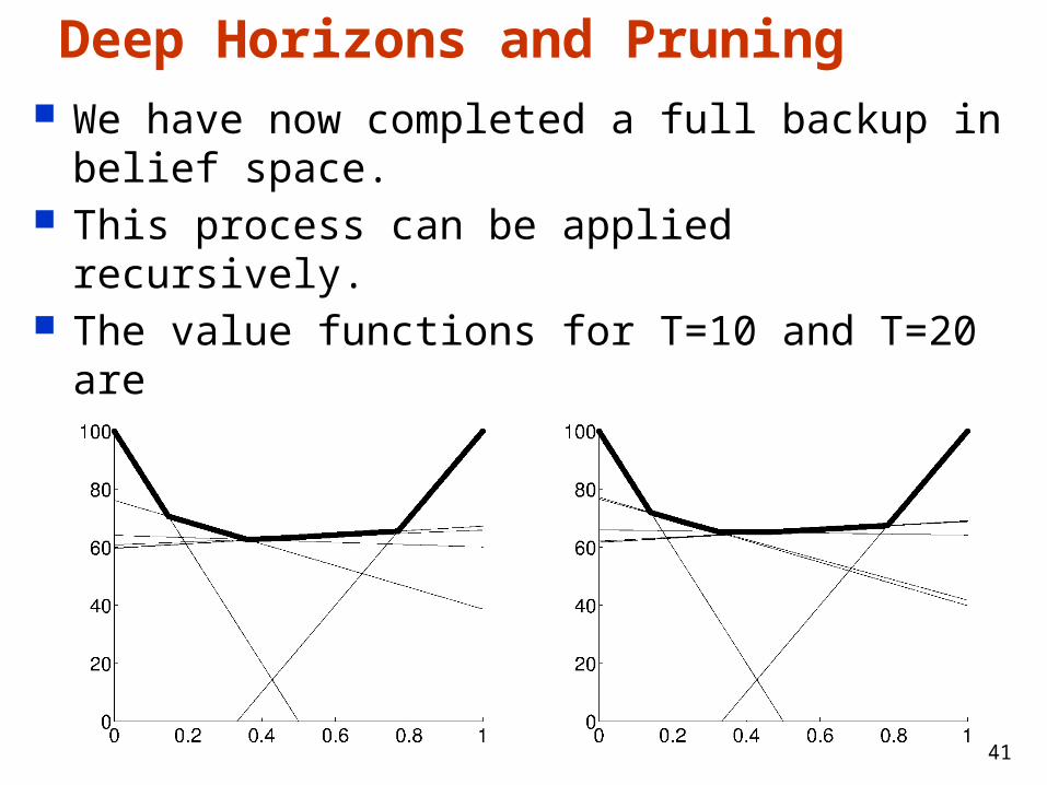
Deep Horizons and Pruning We have now completed a full backup in belief space. This process can be applied recursively. The value functions for T=10 and T=20 are

44

Why Pruning is Essential Each update introduces additional linear

components to V. Each measurement squares the number of

linear components. Thus, an unpruned value function for T=20

includes more than 10547,864 linear functions. At T=30 we have 10561,012,337 linear functions. The pruned value functions at T=20, in

comparison, contains only 12 linear components. The combinatorial explosion of linear components

in the value function are the major reason why POMDPs are impractical for most applications.

45

POMDP Summary

POMDPs compute the optimal action in partially observable, stochastic domains.

For finite horizon problems, the resulting value functions are piecewise linear and convex.

In each iteration the number of linear constraints grows exponentially.

POMDPs so far have only been applied successfully to very small state spaces with small numbers of possible observations and actions.