CSCI-1680 Network Layer:

Intra-domain Routing

Based  partly  on  lecture  notes  by  David  Mazières,  Phil  Levis,  John  Janno<  

Rodrigo Fonseca

Today

•  Intra-Domain Routing •  Next class: Inter-Domain Routing

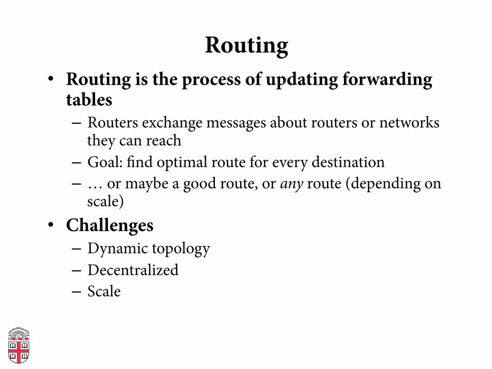
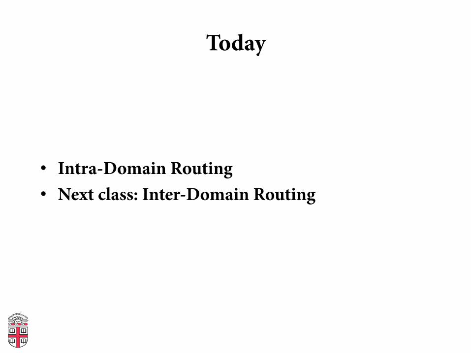
Routing •  Routing is the process of updating forwarding

tables –  Routers exchange messages about routers or networks

they can reach –  Goal: !nd optimal route for every destination –  … or maybe a good route, or any route (depending on

scale) •  Challenges

–  Dynamic topology –  Decentralized –  Scale

Scaling Issues

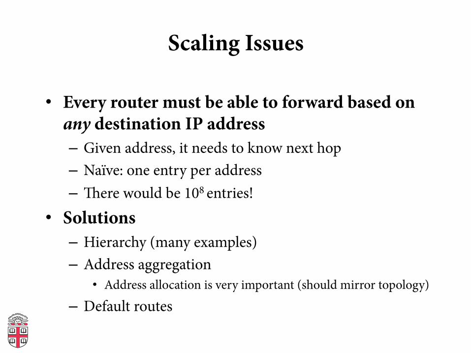
•  Every router must be able to forward based on any destination IP address –  Given address, it needs to know next hop –  Naïve: one entry per address – ere would be 108 entries!

•  Solutions –  Hierarchy (many examples) –  Address aggregation

•  Address allocation is very important (should mirror topology)

–  Default routes

IP Connectivity

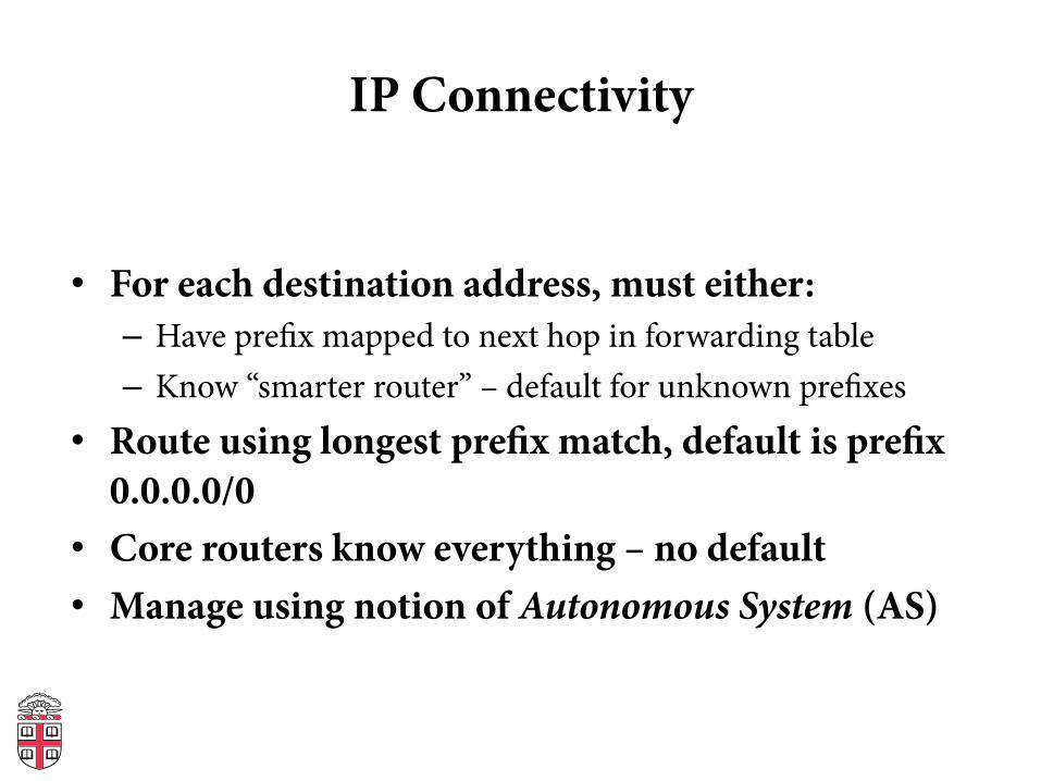
•  For each destination address, must either: –  Have pre!x mapped to next hop in forwarding table –  Know “smarter router” – default for unknown pre!xes

•  Route using longest pre!x match, default is pre!x 0.0.0.0/0

•  Core routers know everything – no default •  Manage using notion of Autonomous System (AS)

NSFNET backboneStanford

BARRNETregional

BerkeleyPARC

NCAR

UA

UNM

Westnetregional

UNL KU

ISU

MidNetregional…

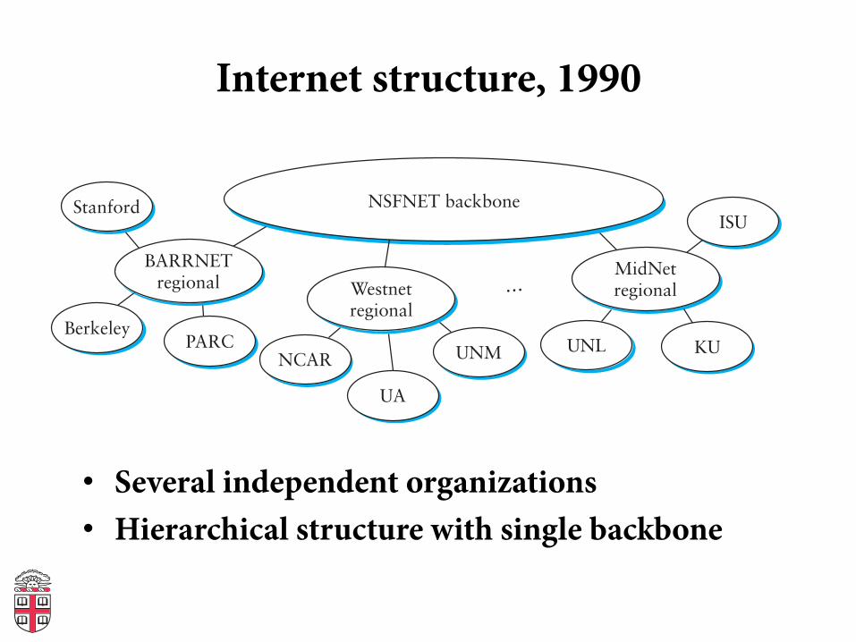
Internet structure, 1990

•  Several independent organizations •  Hierarchical structure with single backbone

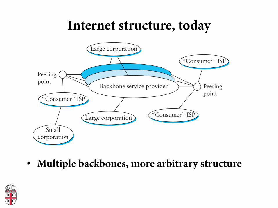
Internet structure, today

•  Multiple backbones, more arbitrary structure

Backbone service provider

Peeringpoint

Peeringpoint

Large corporation

Large corporation

Smallcorporation

“Consumer” ISP

“Consumer” ISP

“Consumer” ISP

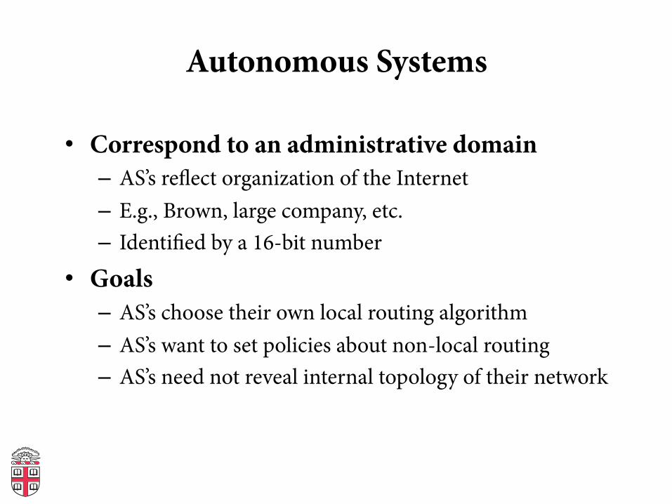
Autonomous Systems

•  Correspond to an administrative domain –  AS’s re#ect organization of the Internet –  E.g., Brown, large company, etc. –  Identi!ed by a 16-bit number

•  Goals –  AS’s choose their own local routing algorithm –  AS’s want to set policies about non-local routing –  AS’s need not reveal internal topology of their network

A R I NAmerican Registry for Internet Numbers

digitalenvoyPROJECT

C o p y r i g h t ( c ) 2 0 0 8 U C R e g e n t sA l l r i g h t s r e s e r v e d .

A R K H O S T S . AARNet . APAN . ARIN . ASTI Institute . CANET . CENIC . CNRST . ELTENET . FunkFeuer . HEANet . Iowa State University . KREONet2 . Purdue University . RNP . TKK . Universitat Leipzig . Universitat Politecnica . University of Cambridge . University of Hawaii . University of Waikato

A C K N O W L E D G E M E N T S F O R I P v 6 . APNIC . AfriNIC . Alexander Gall . Andreas Johansson . Antonio Prado . Antonio Querubin . ARIN . Azael Fernandez Alcantara . Bernhard Schmidt . Brad Dreisbach . Brian Fitzgerald . CAIDA . Chris Morrow . Derek Morr . Gabriel Kerneis . Geoff Huston . Gert Doering . ISC . IIjitsch van Beijnum . Jean-Philippe Pick . John Kristoff . John Osmon . Kenjiro Cho . Kurt Jaeger . LACNIC . Martin Millnert . Mathieu Arnold . RIPE NCC . Nuno Vieira . Ollivier Robert . Sebastian Abt . Shane Kerr

A N A L Y S I S T E A M . Bradley Huffaker . kc claffyS O F T W A R E D E V E L O P M E N T Young Hyun . Matthew LuckieP O S T E R D E S I G N Jennifer Hsu

C O O P E R A T I V E A S S O C I A T I O N F O R I N T E R N E T D A T A A N A L Y S I S

San Diego Supercomputer Center . University of California, San Diego500 Gilman Drive, mc0505 . La Jolla, CA 92093-0505 . 858-534-5000 . http://www.caida.org/

http://www.caida.org/research/topology/as_core_network/

w w w . c a i d a . o r g

01

0W

20W

30W

40W

50W

60W

70W

80W90W100W

110W

120W

130W

140W

150W

160W

17

0W

18

0E/

W1

70

E

160E

150E

140E

130E

120E

110E

100E 90E80E

70E

60E

50E

40E

30E

20E

10

E

OC

E

A

N

I

A

A

FR

IC

A

S

O

U

TH

AM

ER

ICA

A

S

IA

EU

RO

PE

NO

RTH AME

RI

CA

2516(KDDI)2516(KDDI)

1273(CW)1273(CW)5459(London IX)5459(London IX)

3320(Deutsche Telekom)3320(Deutsche Telekom)1299(TeliaNet)1299(TeliaNet)

1239(Sprint)1239(Sprint)3257(Tiscali)3257(Tiscali)

3549(Global Crossing)3549(Global Crossing)7018(AT&T)7018(AT&T)174(Cogent)174(Cogent)

702(MCI)702(MCI)

6453(Teleglobe)6453(Teleglobe)6461(Abovenet)6461(Abovenet)

7132(SBC)7132(SBC)4323(Time Warner)4323(Time Warner)

209(Qwest)209(Qwest)

3561(Savvis)3561(Savvis)

2914(NTT)2914(NTT)

701(UUNET)701(UUNET)3356(Level 3)3356(Level 3)

8928(Interoute)8928(Interoute)

10026(Asia Netcom)10026(Asia Netcom)

7473(Singapore Tel.)7473(Singapore Tel.)

4637(Reach)4637(Reach)

20485(JSC)20485(JSC)

5511(France Tel)5511(France Tel)

15412(Flag)15412(Flag)

3786 (DACOM)3786 (DACOM)

786(JANET)786(JANET)

703 (UUNET)703 (UUNET)

2828 (XO)2828 (XO)3491 (Beyond)3491 (Beyond)

4766 (Korea Tel)4766 (Korea Tel)3904 (Hutchison(3904 (Hutchison)

7714(TelstraClear)7714(TelstraClear)

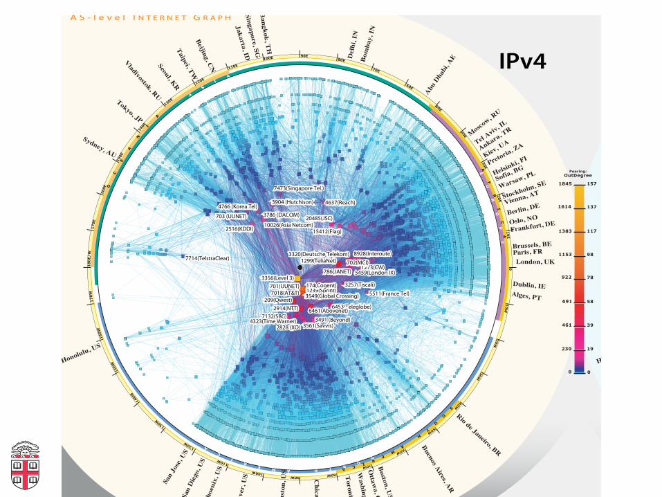
This visualization represents macroscopic snapshots of the IPv4 and IPv6Internet topologies observed during the first week of January 2008.It simultaneously illustrates the peering richness of each topology and the worldwide distribution of nodes in each routing system.

The IPv4 data was collected between January 2nd and 17th 2008 by 13 CAIDA archipelago monitors located in 13 different cities, 11 countries, and 3continents. The monitors probed paths toward 48M /24 networks spread across 95% of the prefixes seen in Route Views Border Gateway Protocol (BGP) routing tables on 1 January 2008.

The IPv6 data was collected between January 1st and 8th 2008 by volunteers responding to a request sent to the North American Network Operators' Group (NANOG) mailing list. There were 56 contributors, in 53 different cities, 9 countries, and

3 continents. They used the scamper command-line tool to probe 2,358 IPv6 destinations spread across 822 prefixes or 81% of the prefixes seen by RIPE NCC on 1 January 2008.

We aggregated these network views to construct IPv4 and IPv6 Internet graphs at the Autonomous System (AS) level. Each AS approximately corresponds to an Internet Service Provider (ISP). We map each IP address to the AS responsible for routing traffic to it, i.e., to the origin (end-of-path) AS for the IP prefix representing the best match of this address in BGP routing tables. For the IPv4 graph we used the BGP IPv4 routing table collected by Route Views. For the IPv6 graph we used the IPv6 routing table collected by RIPE NCC.

The position of each AS node is plotted in polar coordinates, position (radius, angle) calculated using the following equations:

The outdegree of an AS node is the number of next-hop ASes that were observed accepting our probe traffic from this AS. The link color reflects outdegree, from lowest (blue) to highest (yellow). Toward the center of the graph we have manually labeled some of the higher degree ASes with their associated ISPs.

To determine the longitude of ASes, we used the IPv4 BGP table from Route Views and mapped each AS to its set of announced IPv4 prefixes. (IPv4 tables are currently much larger, facilitating more accurate inference of geographic coverage of an AS.) We subdivided prefixes into the smallest prefixes that Digital

maximum.outdegree + 11- log( outdegree(AS) + 1 )radius =

( longitude of the AS’s BGP prefixes )in netacqangle =

Number ofIP address

Number ofIP links

Number ofASes

Number ofASlinks

IPv6IPv4

Dates

Jan. 2nd-17th, 2008Jan. 1st-8th, 2008

4,853,9914,752

5,682,41917,036

17,791489

50,3331,904

1845

1614

1383

1153

922

691

461

230

0

Peering:OutDegree

157

137

117

98

78

58

39

19

0

A S - l e v e l I N T E R N E T G R A P H

I P v 4 & I P v 6 I N T E R N E T T O P O L O G Y M A P J A N U A RY 2 0 0 8

0 1

0W

20W

30W 40W

50W 60W 70W 80W 90W

100W

110W

1

20W

1

30W

140W

15

0W

160W

1

70

W

1

80

E/

W

1

70

E

1

60E

15

0E

140

E

130E

1

20E

110E

100E 90E 80E 70E 60E 50E 40E 30E 20E 1

0E

OC

E

A

N

I

A

A

FR

IC

A

S

O

U

TH

AM

ER

IC

A

A

S

IA

EU

RO

PE

NO

RTHAME

RI

CA

Brussels, BE

Oslo, NO

RK,lu

oeS

SU,ululonoH

SU,revne

D

Toronto, C

A

SU,ogei

DnaS

SU,esoJnaS

SU,xineohP

SU,notsuo

H

Chicago, U

S

Ottaw

a, CA

Washington, U

SBoston, U

S

Buenos Aires, AR

Rio de Janeiro, BR

London, UKParis, FR

Berlin, DE

Vienna, ATStockholm

, SESofi

a, BGHel

sinki, FIPre

toria, ZA

Kiev, UA

Warsaw,

PL

Ankara, TR

Tel Aviv, IL

Moscow,RU

AbuDhabi,AEBombay,IN

Delhi, IN

HT,

kokg

naB

GS,e

ropa

gniS

DI,a

trak

aJ

NC,

gniji

eBWT

,iepia

T

PJ,oyk

oT

UA,yen

dyS

Frankfurt, DE

UR,k

otsovi

dalV

Alges, PT

Dublin, IE

LambdaNet (13237)LambdaNet (13237)

Global (3549)Global (3549)Sprint (6175)Sprint (6175) Teleglobe (6453)Teleglobe (6453)

TowardEX (30071)TowardEX (30071)Hurricane (6939)Hurricane (6939)

Tiscali (3257)Tiscali (3257)NTT (2914)NTT (2914)

IIJ (2497)IIJ (2497)

WIDE (2500)WIDE (2500)

Asia Netcom (18084)Asia Netcom (18084)OpenCarrier (41692)OpenCarrier (41692)

Cable & Wireless (1273)Cable & Wireless (1273)

LavaNet (6435)LavaNet (6435)

Envoy's Netacuity (R) mapped to a single geographic location in January 2008. We calculated the AS angle coordinate from the weighted average (by number of IP addresses in each mapped prefix) of the longitude coordinates of these prefixes.

The IPv6 graph with 486 ASes remains much smaller than the IPv4 graph with 18,753 ASes. While the IPv4 graph's central core is still dominated by American ASes, the IPv6 graph center is more balanced between America and Europe. A European ISP Tiscali (3257) has replaced the previously highest ranking AS, NTT (2914), since our last IPv6 Internet AS core graph in 2005. Although NTT is a Japanese telecommunication company, the address space it uses for AS 2914 comes from the American company Verio, which NTT purchased in 2000. The fact that the largest AS in the IPv6 graph is European and that the other European ASes are comparable in degree to the American ASes reflects the wider adoption of IPv6 outside the United States.

Brussels, BE

Oslo, NO

RK,lu

oeS

SU,ululonoH

SU,revne

D

Toronto, C

A

SU,ogei

DnaS

SU,esoJnaS

SU,xineohP

SU,notsuo

H

Chicago, U

S

Ottaw

a, CA

Washington, U

SBoston, U

S

Buenos Aires, AR

Rio de Janeiro, BR

London, UKParis, FR

Berlin, DE

Vienna, ATStockholm

, SESofi

a, BGHel

sinki, FIPre

toria, ZA

Kiev, UA

Warsaw,

PL

Ankara, TR

Tel Aviv, IL

Moscow,RU

AbuDhabi,AEBombay,IN

Delhi, IN

HT,

kokg

naB

GS,e

ropa

gniS

DI,a

trak

aJ

NC,

gniji

eBWT

,iepia

T

PJ,oyk

oT

UA,yen

dyS

Frankfurt, DE

UR,k

otsovi

dalV

Alges, PT

Dublin, IE

IPv6IPv4

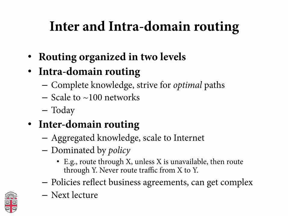
Inter and Intra-domain routing

•  Routing organized in two levels •  Intra-domain routing

–  Complete knowledge, strive for optimal paths –  Scale to ~100 networks –  Today

•  Inter-domain routing –  Aggregated knowledge, scale to Internet –  Dominated by policy

•  E.g., route through X, unless X is unavailable, then route through Y. Never route traffic from X to Y.

–  Policies re#ect business agreements, can get complex –  Next lecture

Intra-Domain Routing

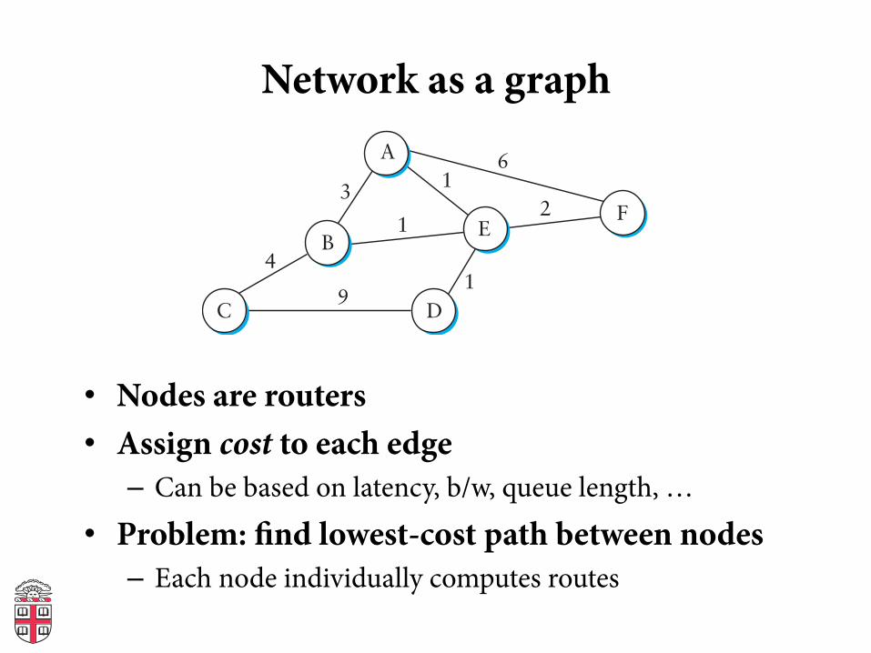
Network as a graph

•  Nodes are routers •  Assign cost to each edge

–  Can be based on latency, b/w, queue length, … •  Problem: !nd lowest-cost path between nodes

–  Each node individually computes routes

4

36

21

9

1

1D

A

FE

B

C

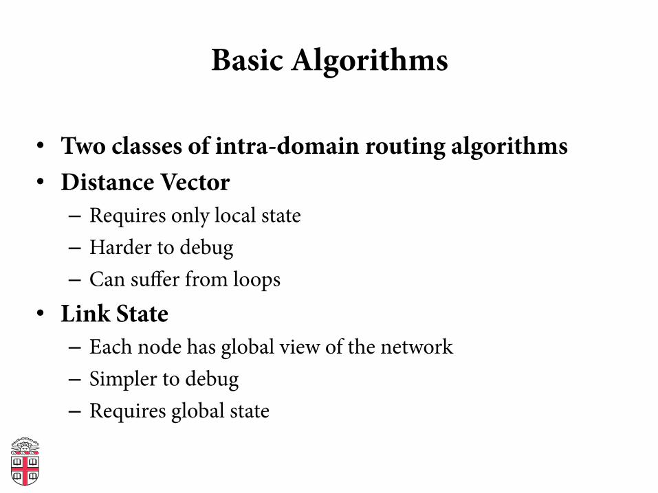
Basic Algorithms

•  Two classes of intra-domain routing algorithms •  Distance Vector –  Requires only local state –  Harder to debug –  Can suffer from loops

•  Link State –  Each node has global view of the network –  Simpler to debug –  Requires global state

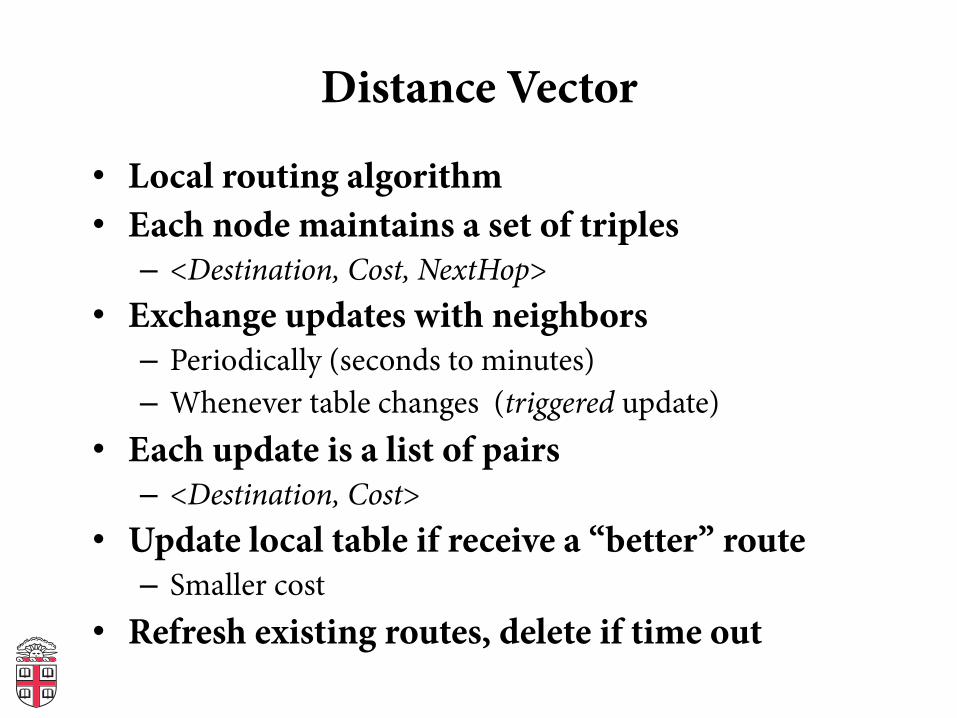
Distance Vector

•  Local routing algorithm •  Each node maintains a set of triples

–  <Destination, Cost, NextHop> •  Exchange updates with neighbors

–  Periodically (seconds to minutes) –  Whenever table changes (triggered update)

•  Each update is a list of pairs –  <Destination, Cost>

•  Update local table if receive a “better” route –  Smaller cost

•  Refresh existing routes, delete if time out

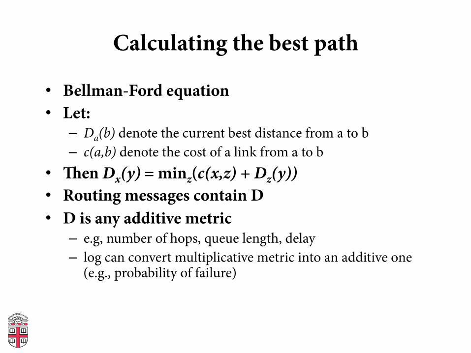
Calculating the best path

•  Bellman-Ford equation •  Let:

–  Da(b) denote the current best distance from a to b –  c(a,b) denote the cost of a link from a to b

•  en Dx(y) = minz(c(x,z) + Dz(y)) •  Routing messages contain D •  D is any additive metric

–  e.g, number of hops, queue length, delay –  log can convert multiplicative metric into an additive one

(e.g., probability of failure)

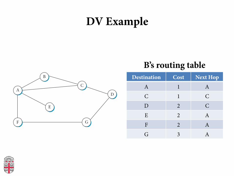
DV Example

Destination Cost Next Hop A 1 A C 1 C D 2 C E 2 A F 2 A G 3 A

D

G

A

F

E

B

C

B’s routing table

G,  1,  G  

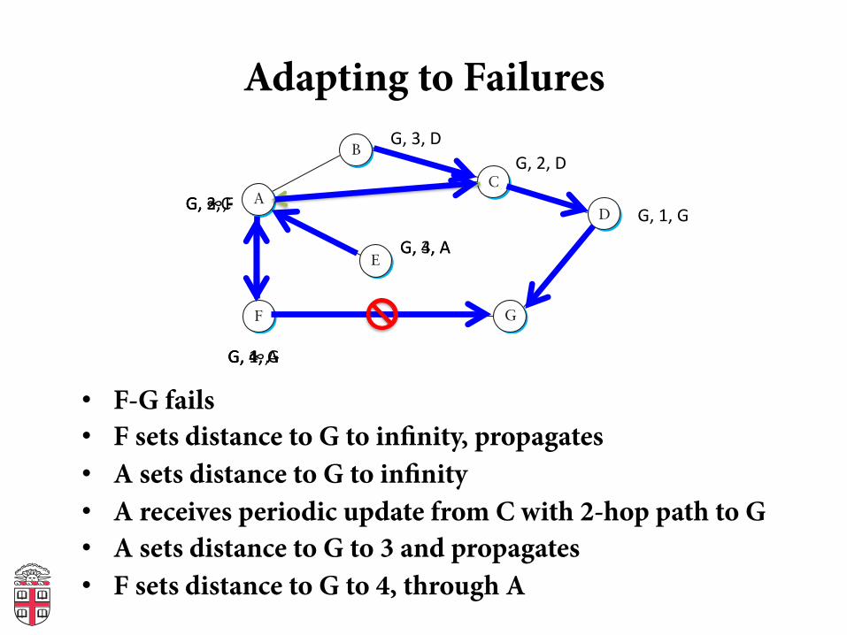
•  F-G fails •  F sets distance to G to in!nity, propagates •  A sets distance to G to in!nity •  A receives periodic update from C with 2-hop path to G •  A sets distance to G to 3 and propagates •  F sets distance to G to 4, through A

G,  ∞,  -­‐  G,  4,  A  

Adapting to Failures

D

G

A

F

E

B

CG,  2,  F  

G,  2,  D  G,  3,  D  

G,  3,  A  

G,  1,  G  G,  ∞,-­‐  G,  3,C  

G,  4,  A  

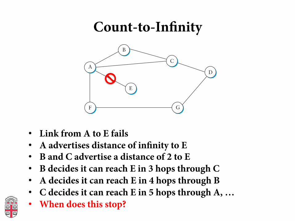
Count-to-In!nity

•  Link from A to E fails •  A advertises distance of in!nity to E •  B and C advertise a distance of 2 to E •  B decides it can reach E in 3 hops through C •  A decides it can reach E in 4 hops through B •  C decides it can reach E in 5 hops through A, … •  When does this stop?

D

G

A

F

E

B

C

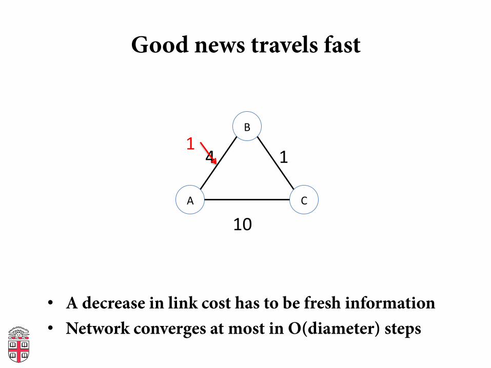
Good news travels fast

A  

B  

C  

4   1  

10  

1  

•  A decrease in link cost has to be fresh information •  Network converges at most in O(diameter) steps

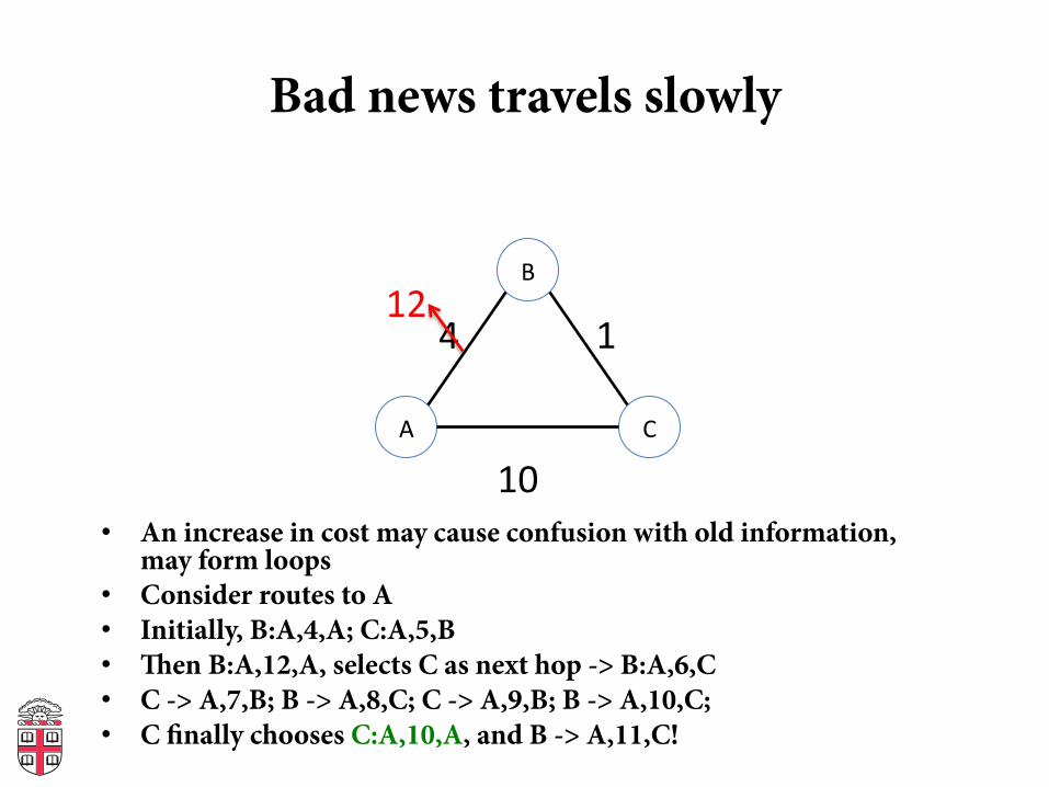
Bad news travels slowly

A  

B  

C  

4   1  

10  

12  

•  An increase in cost may cause confusion with old information, may form loops

•  Consider routes to A •  Initially, B:A,4,A; C:A,5,B •  en B:A,12,A, selects C as next hop -> B:A,6,C •  C -> A,7,B; B -> A,8,C; C -> A,9,B; B -> A,10,C; •  C !nally chooses C:A,10,A, and B -> A,11,C!

How to avoid loops

•  IP TTL !eld prevents a packet from living forever –  Does not repair a loop

•  Simple approach: consider a small cost n (e.g., 16) to be in!nity –  Aer n rounds decide node is unavailable –  But rounds can be long, this takes time

•  Problem: distance vector based only on local information

Better loop avoidance

•  Split Horizon –  When sending updates to node A, don’t include routes

you learned from A –  Prevents B and C from sending cost 2 to A

•  Split Horizon with Poison Reverse –  Rather than not advertising routes learned from A,

explicitly include cost of ∞. –  Faster to break out of loops, but increases

advertisement sizes

Warning

•  Split horizon/split horizon with poison reverse only help between two nodes –  Can still get loop with three nodes involved –  Might need to delay advertising routes aer changes,

but affects convergence time

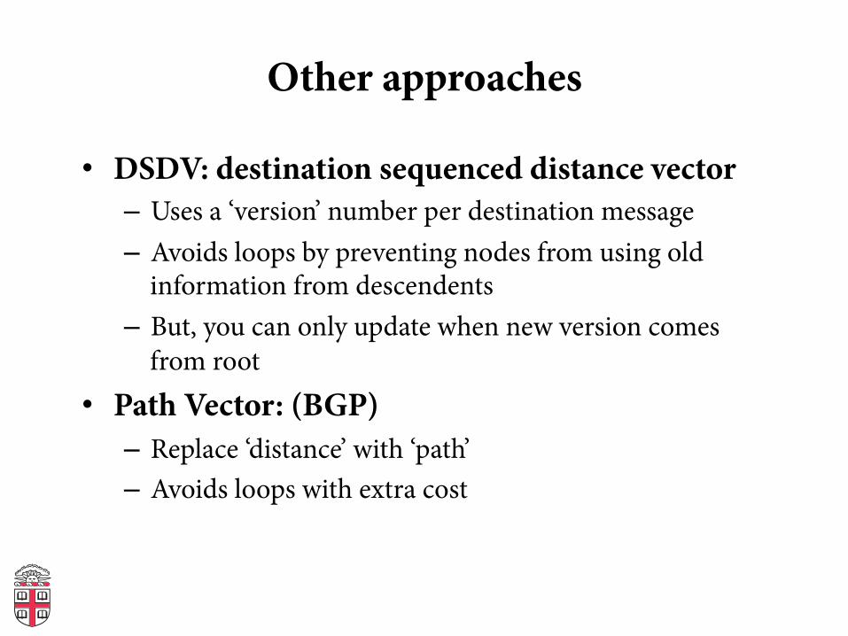
Other approaches

•  DSDV: destination sequenced distance vector –  Uses a ‘version’ number per destination message –  Avoids loops by preventing nodes from using old

information from descendents –  But, you can only update when new version comes

from root •  Path Vector: (BGP)

–  Replace ‘distance’ with ‘path’ –  Avoids loops with extra cost

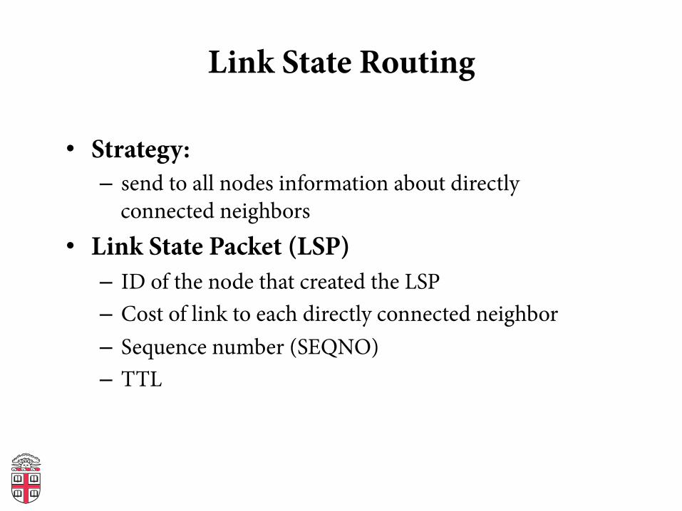
Link State Routing

•  Strategy: –  send to all nodes information about directly

connected neighbors •  Link State Packet (LSP)

–  ID of the node that created the LSP –  Cost of link to each directly connected neighbor –  Sequence number (SEQNO) –  TTL

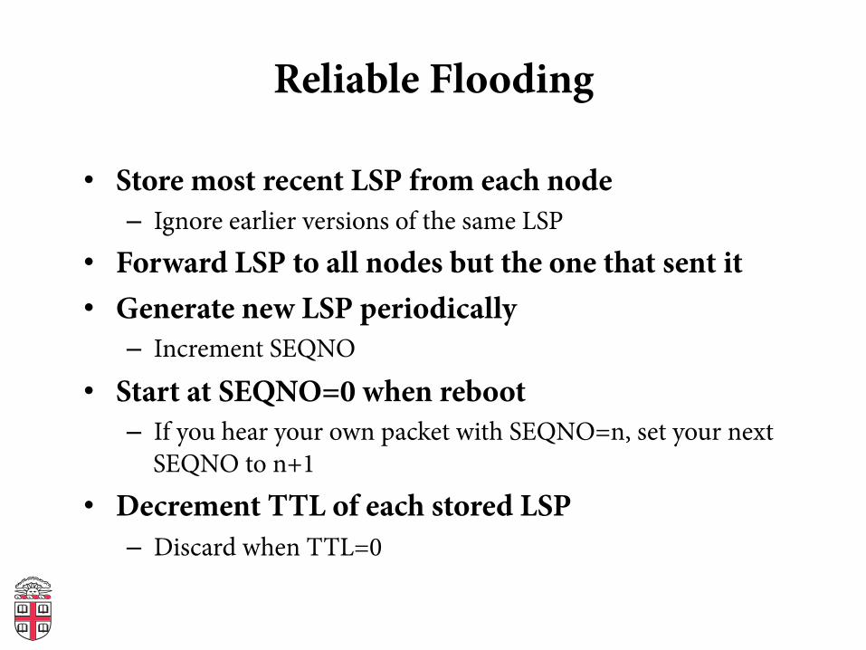
Reliable Flooding

•  Store most recent LSP from each node –  Ignore earlier versions of the same LSP

•  Forward LSP to all nodes but the one that sent it •  Generate new LSP periodically

–  Increment SEQNO

•  Start at SEQNO=0 when reboot –  If you hear your own packet with SEQNO=n, set your next

SEQNO to n+1 •  Decrement TTL of each stored LSP

–  Discard when TTL=0

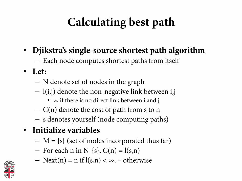
Calculating best path

•  Djikstra’s single-source shortest path algorithm –  Each node computes shortest paths from itself

•  Let: –  N denote set of nodes in the graph –  l(i,j) denote the non-negative link between i,j

•  ∞ if there is no direct link between i and j –  C(n) denote the cost of path from s to n –  s denotes yourself (node computing paths)

•  Initialize variables –  M = {s} (set of nodes incorporated thus far) –  For each n in N-{s}, C(n) = l(s,n) –  Next(n) = n if l(s,n) < ∞, – otherwise

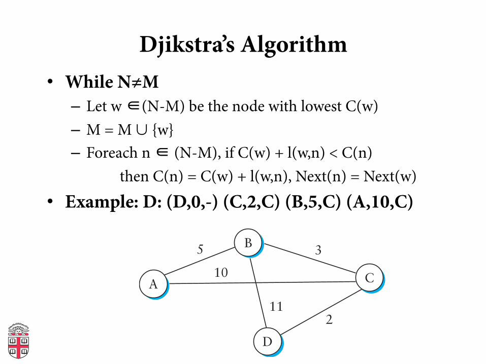
Djikstra’s Algorithm •  While N≠M

–  Let w ∈(N-M) be the node with lowest C(w) –  M = M ∪ {w} –  Foreach n ∈ (N-M), if C(w) + l(w,n) < C(n)

then C(n) = C(w) + l(w,n), Next(n) = Next(w) •  Example: D: (D,0,-) (C,2,C) (B,5,C) (A,10,C)

D

A

B

C

5 3

211

10

Distance Vector vs. Link State

•  # of messages (per node) –  DV: O(d), where d is degree of node –  LS: O(nd) for n nodes in system

•  Computation –  DV: convergence time varies (e.g., count-to-in!nity) –  LS: O(n2) with O(nd) messages

•  Robustness: what happens with malfunctioning router? –  DV: Nodes can advertise incorrect path cost –  DV: Others can use the cost, propagates through network –  LS: Nodes can advertise incorrect link cost

Metrics •  Original ARPANET metric

–  measures number of packets enqueued in each link –  neither latency nor bandwidth in consideration

•  New ARPANET metric –  Stamp arrival time (AT) and departure time (DT) –  When link-level ACK arrives, compute

Delay = (DT – AT) + Transmit + Latency –  If timeout, reset DT to departure time for retransmission –  Link cost = average delay over some time period

•  Fine Tuning –  Compressed dynamic range –  Replaced Delay with link utilization

•  Today: commonly set manually to achieve speci!c goals

Examples

•  RIPv2 –  Fairly simple implementation of DV –  RFC 2453 (38 pages)

•  OSPF (Open Shortest Path First) –  More complex link-state protocol –  Adds notion of areas for scalability –  RFC 2328 (244 pages)

RIPv2

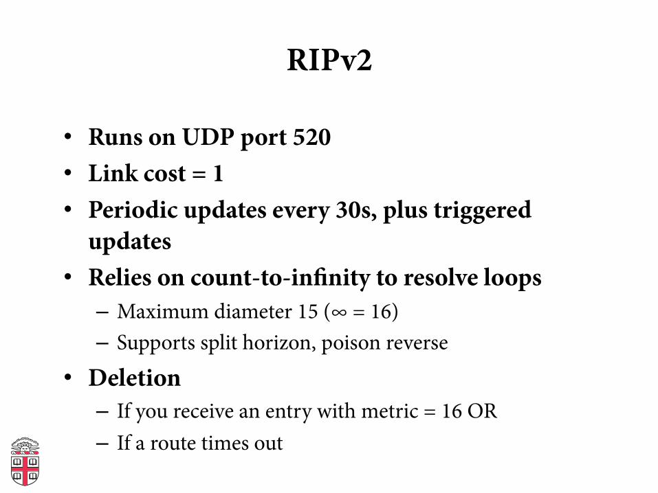
•  Runs on UDP port 520 •  Link cost = 1 •  Periodic updates every 30s, plus triggered

updates •  Relies on count-to-in!nity to resolve loops

–  Maximum diameter 15 (∞ = 16) –  Supports split horizon, poison reverse

•  Deletion –  If you receive an entry with metric = 16 OR –  If a route times out

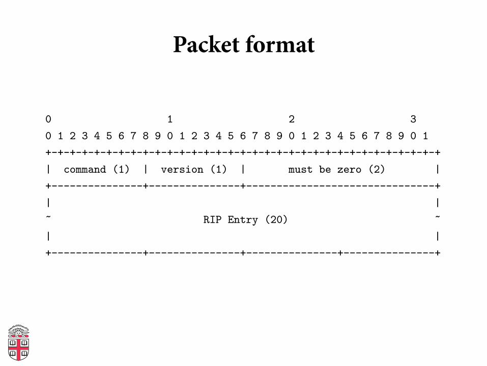
Packet format RIPv2 packet format

0 1 2 3

0 1 2 3 4 5 6 7 8 9 0 1 2 3 4 5 6 7 8 9 0 1 2 3 4 5 6 7 8 9 0 1

+-+-+-+-+-+-+-+-+-+-+-+-+-+-+-+-+-+-+-+-+-+-+-+-+-+-+-+-+-+-+-+-+

| command (1) | version (1) | must be zero (2) |

+---------------+---------------+-------------------------------+

| |

~ RIP Entry (20) ~

| |

+---------------+---------------+---------------+---------------+

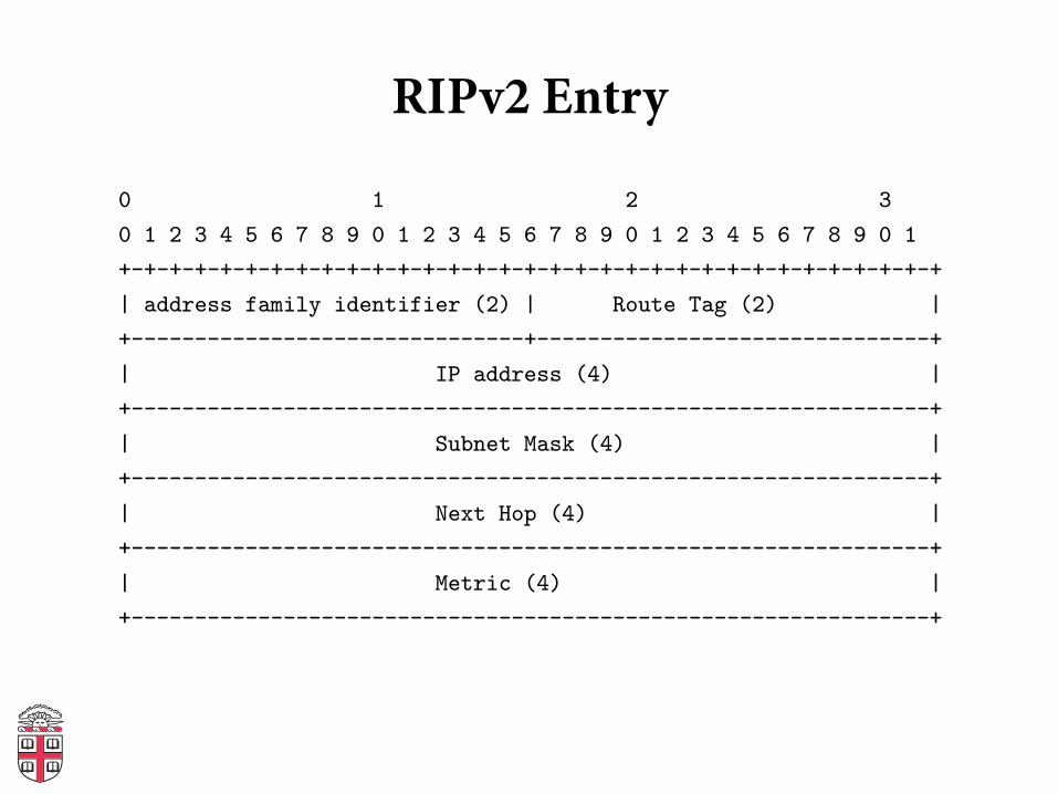
RIPv2 Entry RIPv2 Entry

0 1 2 3

0 1 2 3 4 5 6 7 8 9 0 1 2 3 4 5 6 7 8 9 0 1 2 3 4 5 6 7 8 9 0 1

+-+-+-+-+-+-+-+-+-+-+-+-+-+-+-+-+-+-+-+-+-+-+-+-+-+-+-+-+-+-+-+-+

| address family identifier (2) | Route Tag (2) |

+-------------------------------+-------------------------------+

| IP address (4) |

+---------------------------------------------------------------+

| Subnet Mask (4) |

+---------------------------------------------------------------+

| Next Hop (4) |

+---------------------------------------------------------------+

| Metric (4) |

+---------------------------------------------------------------+

Route Tag !eld

•  Allows RIP nodes to distinguish internal and external routes

•  Must persist across announcements •  E.g., encode AS

Next Hop !eld

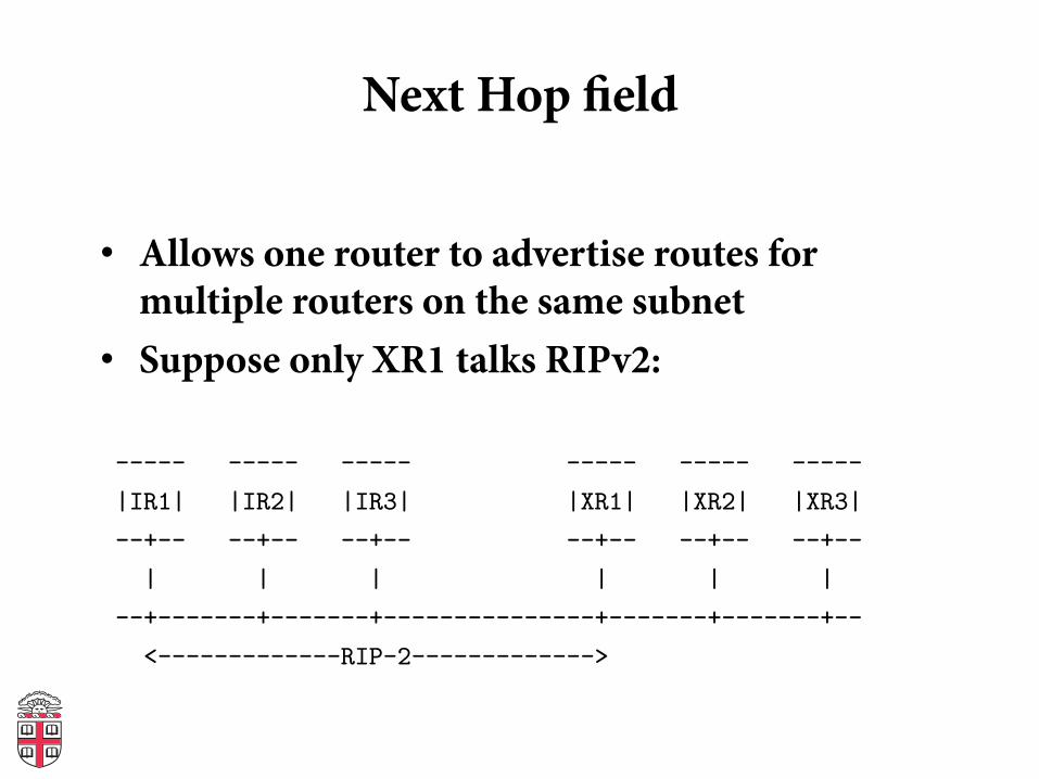
•  Allows one router to advertise routes for multiple routers on the same subnet

•  Suppose only XR1 talks RIPv2:

Next Hop Field

• Allows one router to advertise routes for multiplerouters on same subnet

• Suppose only XR1 talks RIP2:----- ----- ----- ----- ----- -----

|IR1| |IR2| |IR3| |XR1| |XR2| |XR3|

--+-- --+-- --+-- --+-- --+-- --+--

| | | | | |

--+-------+-------+---------------+-------+-------+--

<-------------RIP-2------------->

OSPFv2

•  Link state protocol •  Runs directly over IP (protocol 89)

–  Has to provide its own reliability

•  All exchanges are authenticated •  Adds notion of areas for scalability

OSPF Areas

•  Area 0 is “backbone” area (includes all boundary routers)

•  Traffic between two areas must always go through area 0

•  Only need to know how to route exactly within area

•  Otherwise, just route to the appropriate area •  Tradeoff: scalability versus optimal routes

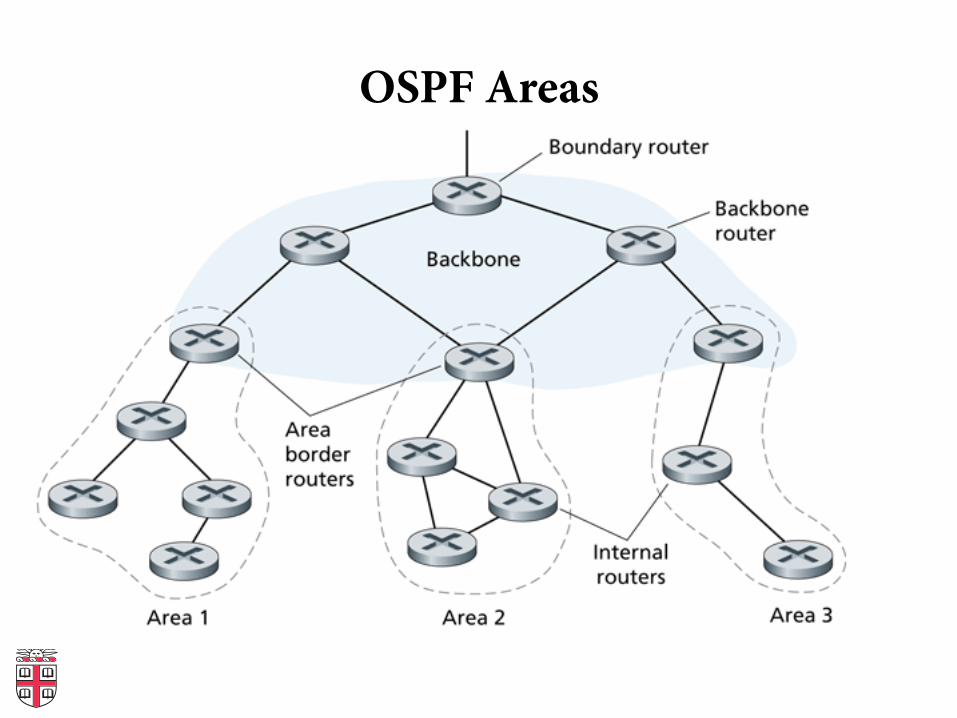
OSPF Areas OSPF areas

Next Class

•  Inter-domain routing: how scale routing to the entire Internet