CSC321 Lecture 18: Mixture Modelingrgrosse/courses/csc321_2017/slides/... · 2017-03-22 ·...

CSC321 Lecture 18: Mixture Modeling

Roger Grosse

Roger Grosse CSC321 Lecture 18: Mixture Modeling 1 / 27

Overview

Some examples of situations where you’d use unupservised learning

You want to understand how a scientific field has changed over time.You want to take a large database of papers and model how thedistribution of topics changes from year to year. But what are thetopics?You’re a biologist studying animal behavior, so you want to infer ahigh-level description of their behavior from video. You don’t know theset of behaviors ahead of time.You want to reduce your energy consumption, so you take a time seriesof your energy consumption over time, and try to break it down intoseparate components (refrigerator, washing machine, etc.).

Common theme: you have some data, and you want to infer thecausal structure underlying the data.

This structure is latent, which means it’s never observed.


Overview

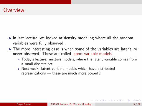
In last lecture, we looked at density modeling where all the randomvariables were fully observed.

The more interesting case is when some of the variables are latent, ornever observed. These are called latent variable models.

Today’s lecture: mixture models, where the latent variable comes froma small discrete setNext week: latent variable models which have distributedrepresentations — these are much more powerful


Clustering

Sometimes the data form clusters, where examples within a cluster aresimilar to each other, and examples in different clusters are dissimilar:

Such a distribution is multimodal, since it has multiple modes, orregions of high probability mass.

Grouping data points into clusters, with no labels, is called clustering

E.g. clustering machine learning papers based on topic (deep learning,Bayesian models, etc.)

This is an overly simplistic model — more on that later


K-Means

First, let’s look at a simple clustering algorithm, called k-means.This is an iterative algorithm. In each iteration, we keep track of:

An assignment of data points to clustersThe center of each cluster

Start with random cluster locations, then alternate between:Assignment step: assign each data point to the nearest clusterRefitting step: move each cluster center to the average of its datapoints


K-Means

Each iteration can be shown to decrease a particular cost function: the sum of

squared distances from data points to their corresponding cluster centers.

More on this in CSC411.Problem: what if the clusters aren’t spherical?

Let’s instead treat clustering as a distribution modeling problem.

Last lecture, we fit Gaussian distributions to data.To model multimodal distributions, let’s fit a mixture model, whereeach data point belongs to a different component.E.g., in a mixture of Gaussians, each data point comes from one ofseveral different Gaussian distributions.We don’t need to use Gaussians — we can pick whatever distributionbest represents our data.


Mixture of Gaussians

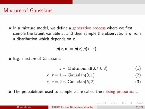
In a mixture model, we define a generative process where we firstsample the latent variable z , and then sample the observations x froma distribution which depends on z .

p(z , x) = p(z) p(x | z).

E.g. mixture of Gaussians:

z ∼ Multinomial(0.7, 0.3) (1)

x | z = 1 ∼ Gaussian(0, 1) (2)

x | z = 2 ∼ Gaussian(6, 2) (3)

The probabilities used to sample z are called the mixing proportions.


Mixture of Gaussians

Example:

The probability density function over x is defined by marginalizing, orsumming out, z :

p(x) =K∑

k=1

Pr(z = k) p(x | z = k)


Posterior Inference

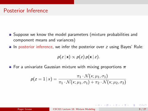
Suppose we know the model parameters (mixture probabilities andcomponent means and variances)

In posterior inference, we infer the posterior over z using Bayes’ Rule:

p(z | x) ∝ p(z) p(x | z).

For a univariate Gaussian mixture with mixing proportions π

p(z = 1 | x) =π1 · N (x ;µ1, σ1)

π1 · N (x ;µ1, σ1) + π2 · N (x ;µ2, σ2)


Posterior Inference

Example:


Posterior Inference

Sometimes the observables aren’t actually observed — then we saythey’re missingOne use of probabilistic models is to make predictions about missingdata

E.g. image completion, which you’ll do in Assignment 4

Analogously to Bayesian parameter estimation, we use the posteriorpredictive distribution:

p(x2 | x1) =∑z

p(z | x1)︸︷︷︸posterior

p(x2 | z , x1).

If the dimensions of x are conditionally independent given z , this isjust a reweighting of the original mixture model, where we use theposterior rather than the prior.

p(x2 | x1) =∑z

p(z | x1)︸︷︷︸posterior

p(x2 | z)︸︷︷︸component PDF

.


Posterior Inference

Example:

Fully worked-through example in the lecture notes.


Parameter Learning

Now let’s talk about learning. We need to fit two sets of paramters:

The mixture probabilities πk = Pr(z = k)The mean µk and standard deviation σk for each component

If someone hands us the values of all the latent variables, it’s easy tofit the parameters using maximum likelihood.

` = logN∏i=1

p(z(i), x (i))

= logN∏i=1

p(z(i))p(x (i) | z(i))

=N∑i=1

log p(z(i))︸︷︷︸π

+ log p(x (i) | z(i))︸︷︷︸µk , σk


Parameter Learning

Let r(i)k be the indicator variable for z(i) = k . This is called the

responsibilitiy

Solving for the mixing probabilities:

` =N∑i=1

log p(z(i)) + log p(x (i) | z(i))

= const +N∑i=1

log p(z(i))

This is just the maximum likelihood problem for the multinomialdistirbution. The solution is just the empirical proabilities, which wecan write as:

πk ←1

N

N∑i=1

r(i)k


Parameter Learning

Solving for the mean parameter µk for component k :

` =N∑i=1

log p(z (i)) + log p(x (i) | z (i))

= const +N∑i=1

log p(x (i) | z (i))

= const +N∑i=1

r(i)k logN (x (i);µk , σk)

This is just maximum likelihood for the parameters of a Gaussiandistribution, where only certain data points count.

Solution:

µk ←∑N

i=1 r(i)k x (i)∑N

i=1 r(i)k


Expectation-Maximization

We’ve seen how to do two things:

Given the model parameters, compute the posterior over the latentvariablesGiven the latent variables, find the maximum likelihood parameters

But we don’t know the parameters or latent variables, so we have achicken-and-egg problem.

Remember k-means? We iterated between an assignment step and arefitting step.

Expectation-Maximization (E-M) is an analogous procedure whichalternates bewteen two steps:

Expectation step (E-step): Compute the posterior expectations ofthe latent variables zMaximization step (M-step): Solve for the maximum likelihoodparameters given the full set of x ’s and z ’s



E-step:

This is like the assignment step in k-means, except that we assignfractional responsibilities.

r(i)k ← Pr(z(i) = k | x (i))∝ πk · N (x (i);µk , σk)

This is just posterior inference, which we’ve already talked about.



M-step:

Maximum likelihood with fractional counts:

θ ← arg maxθ

N∑i=1

K∑k=1

r(i)k

[logPr(z(i) = k) + log p(x(i) | z(i) = k)

]The maximum likelihood formulas we already saw don’t depend onthe responsibilities being 0 or 1. They also work with fractionalresponsibilities. E.g.,

πk ←1

N

N∑i=1

r(i)k

µk ←∑N

i=1 r(i)k x (i)∑N

i=1 r(i)k



We initialize the model parameters randomly and then repeatedlyapply the E-step and M-step.

Each step can be shown to increase the log-likelihood, but this isbeyond the scope of the class.

Optional mathematical justification in the lecture notes, in case you’reinterested.Also, there’s a full explanation in CSC 411.Next lecture, we’ll fit a different latent variable model by doing gradientdescent on the parameters. This will turn out to have an EM-like flavor.


Example

Suppose we recorded a bunch of temperatures in March for Torontoand Miami, but forgot to record which was which, and they’re alljumbled together.

Let’s try to separate them out using a mixture of Gaussians and E-M.


Example

Random initialization


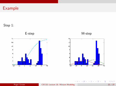
Example

Step 1:

E-step M-step


Example

Step 2:

E-step M-step


Example

Step 3:

E-step M-step


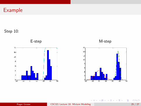
Example

Step 10:

E-step M-step



We used univariate Gaussian components for simplicity, but otherdistributions are possible.

Multivariate Gaussians:

In Programming Assignment 4, you will fit a mixture of Bernoullismodel.


Odds and Ends

E-M can get stuck in local optima.

Initialize from k-means, which can be more robust in practiceUse multiple random restarts and pick the one with the best objectivefunction

Mixture models are a localist representation: the latent variables takevalues in a small discrete set.

We can use more complex distributions over latent variables to get adistributed representation.The difficulty is posterior inference: while this is easy to do exactly formixture models, it’s intractable in general, and we’ll need to makeapproximations.


CSC321 Lecture 18: Mixture Modelingrgrosse/courses/csc321_2017/slides/... · 2017-03-22 ·...

Documents

Transcript of CSC321 Lecture 18: Mixture Modelingrgrosse/courses/csc321_2017/slides/... · 2017-03-22 ·...