CS6220: Data Mining Techniques - CS | Computer...
62
CS6220: DATA MINING TECHNIQUES Instructor: Yizhou Sun [email protected] January 28, 2013 Chapter 7: Advanced Pattern Mining
Transcript of CS6220: Data Mining Techniques - CS | Computer...
CS6220: DATA MINING TECHNIQUES
Instructor: Yizhou Sun [email protected]
January 28, 2013
Chapter 7: Advanced Pattern Mining
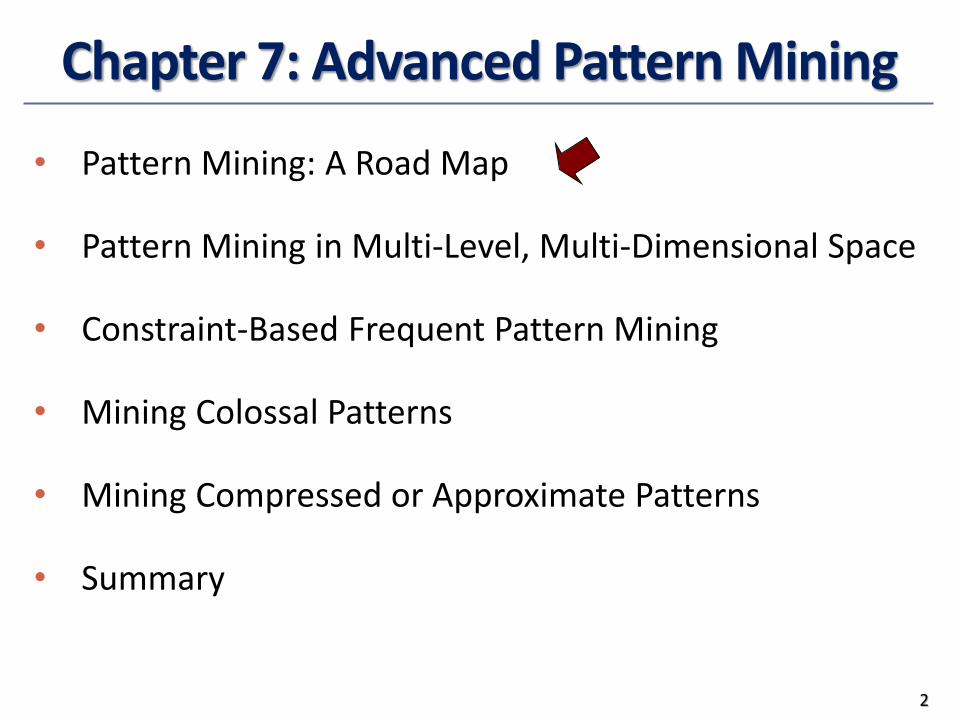
Chapter 7: Advanced Pattern Mining
• Pattern Mining: A Road Map
• Pattern Mining in Multi-Level, Multi-Dimensional Space
• Constraint-Based Frequent Pattern Mining
• Mining Colossal Patterns
• Mining Compressed or Approximate Patterns
• Summary
2
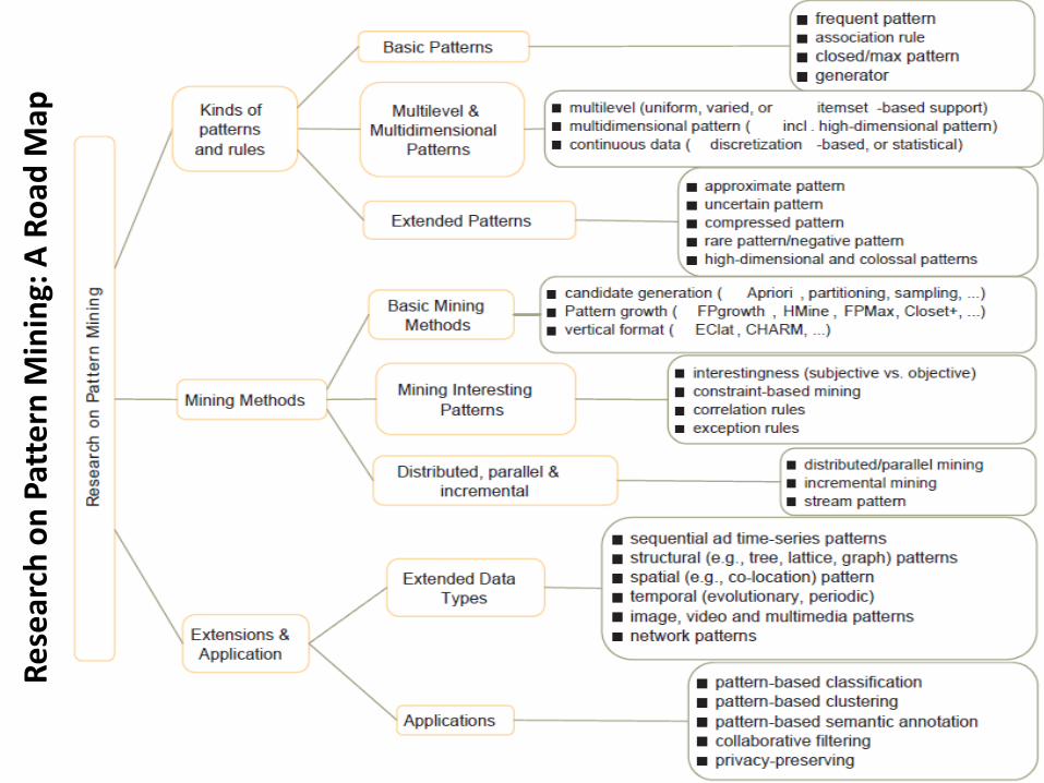
Re
sear
ch o
n P
atte
rn M
inin
g: A
Ro
ad M
ap
3
Chapter 7: Advanced Pattern Mining
• Pattern Mining: A Road Map
• Pattern Mining in Multi-Level, Multi-Dimensional Space
• Mining Multi-Level Association
• Mining Multi-Dimensional Association
• Mining Quantitative Association Rules
• Mining Rare Patterns and Negative Patterns
• Constraint-Based Frequent Pattern Mining
• Mining Colossal Patterns
• Mining Compressed or Approximate Patterns
• Summary
4
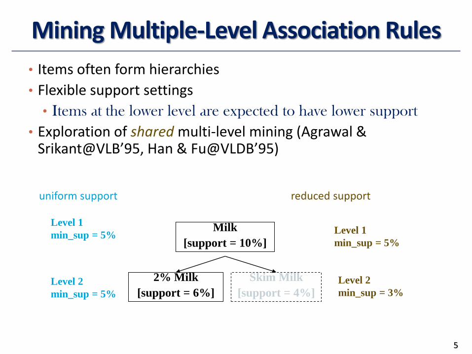
Mining Multiple-Level Association Rules
• Items often form hierarchies
• Flexible support settings
• Items at the lower level are expected to have lower support
• Exploration of shared multi-level mining (Agrawal & Srikant@VLB’95, Han & Fu@VLDB’95)
5
uniform support
Milk
[support = 10%]
2% Milk
[support = 6%]
Skim Milk
[support = 4%]
Level 1
min_sup = 5%
Level 2
min_sup = 5%
Level 1
min_sup = 5%
Level 2
min_sup = 3%
reduced support
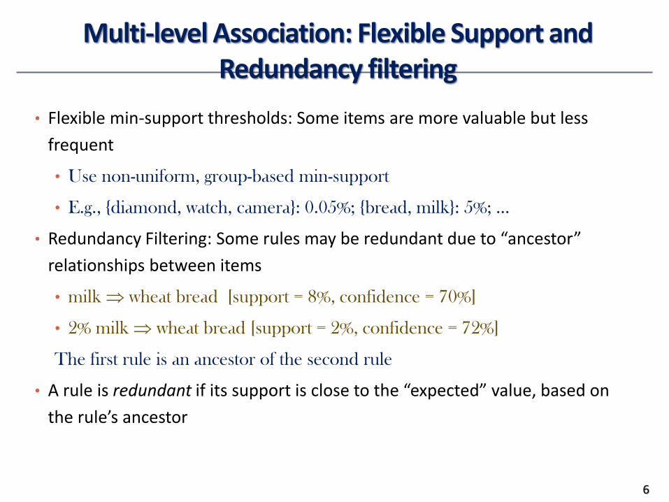
Multi-level Association: Flexible Support and Redundancy filtering
• Flexible min-support thresholds: Some items are more valuable but less
frequent
• Use non-uniform, group-based min-support
• E.g., {diamond, watch, camera}: 0.05%; {bread, milk}: 5%; …
• Redundancy Filtering: Some rules may be redundant due to “ancestor”
relationships between items
• milk wheat bread [support = 8%, confidence = 70%]
• 2% milk wheat bread [support = 2%, confidence = 72%]
The first rule is an ancestor of the second rule
• A rule is redundant if its support is close to the “expected” value, based on
the rule’s ancestor
6
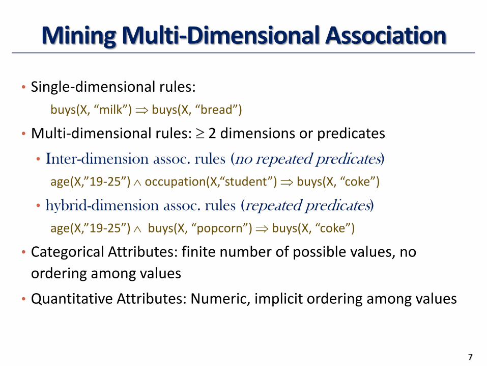
Mining Multi-Dimensional Association
• Single-dimensional rules:
buys(X, “milk”) buys(X, “bread”)
• Multi-dimensional rules: 2 dimensions or predicates
• Inter-dimension assoc. rules (no repeated predicates)
age(X,”19-25”) occupation(X,“student”) buys(X, “coke”)
• hybrid-dimension assoc. rules (repeated predicates)
age(X,”19-25”) buys(X, “popcorn”) buys(X, “coke”)
• Categorical Attributes: finite number of possible values, no
ordering among values
• Quantitative Attributes: Numeric, implicit ordering among values
7
Mining Quantitative Associations
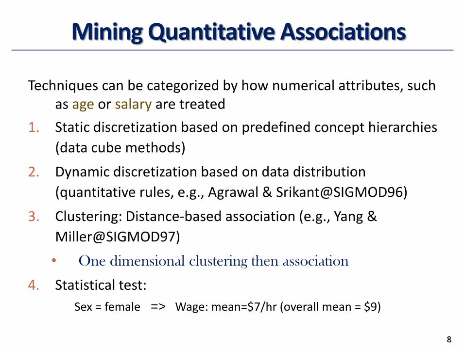
Techniques can be categorized by how numerical attributes, such as age or salary are treated
1. Static discretization based on predefined concept hierarchies
(data cube methods)
2. Dynamic discretization based on data distribution
(quantitative rules, e.g., Agrawal & Srikant@SIGMOD96)
3. Clustering: Distance-based association (e.g., Yang &
Miller@SIGMOD97)
• One dimensional clustering then association
4. Statistical test:
Sex = female => Wage: mean=$7/hr (overall mean = $9)
8
Negative and Rare Patterns
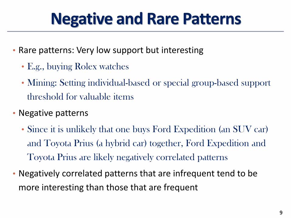
• Rare patterns: Very low support but interesting
• E.g., buying Rolex watches
• Mining: Setting individual-based or special group-based support
threshold for valuable items
• Negative patterns
• Since it is unlikely that one buys Ford Expedition (an SUV car)
and Toyota Prius (a hybrid car) together, Ford Expedition and
Toyota Prius are likely negatively correlated patterns
• Negatively correlated patterns that are infrequent tend to be
more interesting than those that are frequent
9
10
Defining Negative Correlated Patterns (I)
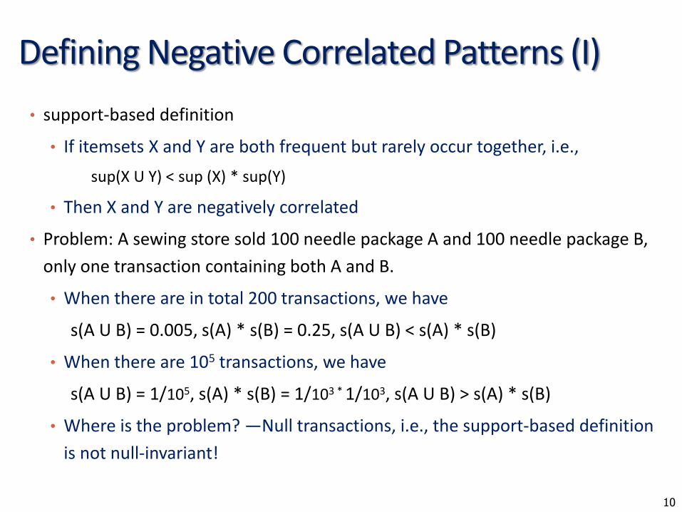
• support-based definition
• If itemsets X and Y are both frequent but rarely occur together, i.e.,
sup(X U Y) < sup (X) * sup(Y)
• Then X and Y are negatively correlated
• Problem: A sewing store sold 100 needle package A and 100 needle package B,
only one transaction containing both A and B.
• When there are in total 200 transactions, we have
s(A U B) = 0.005, s(A) * s(B) = 0.25, s(A U B) < s(A) * s(B)
• When there are 105 transactions, we have
s(A U B) = 1/105, s(A) * s(B) = 1/103 * 1/103, s(A U B) > s(A) * s(B)
• Where is the problem? —Null transactions, i.e., the support-based definition
is not null-invariant!
11
Defining Negative Correlated Patterns (II)
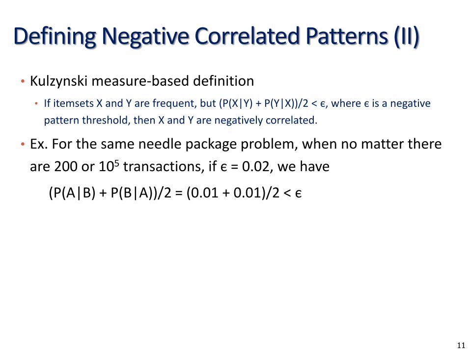
• Kulzynski measure-based definition
• If itemsets X and Y are frequent, but (P(X|Y) + P(Y|X))/2 < є, where є is a negative
pattern threshold, then X and Y are negatively correlated.
• Ex. For the same needle package problem, when no matter there
are 200 or 105 transactions, if є = 0.02, we have
(P(A|B) + P(B|A))/2 = (0.01 + 0.01)/2 < є
Chapter 7: Advanced Pattern Mining
• Pattern Mining: A Road Map
• Pattern Mining in Multi-Level, Multi-Dimensional Space
• Constraint-Based Frequent Pattern Mining
• Mining Colossal Patterns
• Mining Compressed or Approximate Patterns
• Summary
12
Constraint-based (Query-Directed) Mining
• Finding all the patterns in a database autonomously? — unrealistic!
• The patterns could be too many but not focused!
• Data mining should be an interactive process
• User directs what to be mined using a data mining query language (or a
graphical user interface)
• Constraint-based mining
• User flexibility: provides constraints on what to be mined
• Optimization: explores such constraints for efficient mining — constraint-
based mining: constraint-pushing, similar to push selection first in DB query
processing
• Note: still find all the answers satisfying constraints, not finding some answers
in “heuristic search”
13
Constraints in Data Mining
• Knowledge type constraint:
• classification, association, etc.
• Data constraint — using SQL-like queries
• find product pairs sold together in stores in Chicago this year
• Dimension/level constraint
• in relevance to region, price, brand, customer category
• Interestingness constraint
• strong rules: min_support 3%, min_confidence 60%
• Rule (or pattern) constraint
• small sales (price < $10) triggers big sales (sum > $200)
14
Meta-Rule Guided Mining
• Meta-rule can be in the rule form with partially instantiated predicates and constants
P1(X, Y) ^ P2(X, W) => buys(X, “iPad”)
• The resulting rule derived can be
age(X, “15-25”) ^ profession(X, “student”) => buys(X, “iPad”)
• In general, it can be in the form of
P1 ^ P2 ^ … ^ Pl => Q1 ^ Q2 ^ … ^ Qr
15
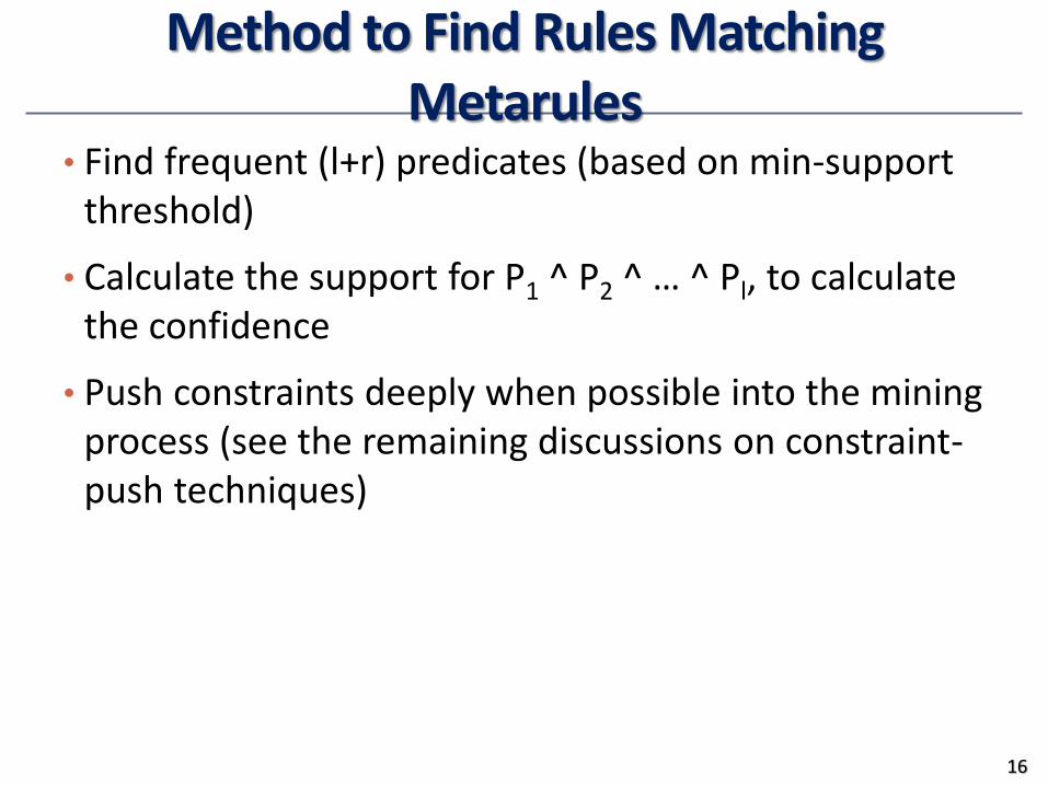
Method to Find Rules Matching Metarules
• Find frequent (l+r) predicates (based on min-support threshold)
• Calculate the support for P1 ^ P2 ^ … ^ Pl, to calculate the confidence
• Push constraints deeply when possible into the mining process (see the remaining discussions on constraint-push techniques)
16
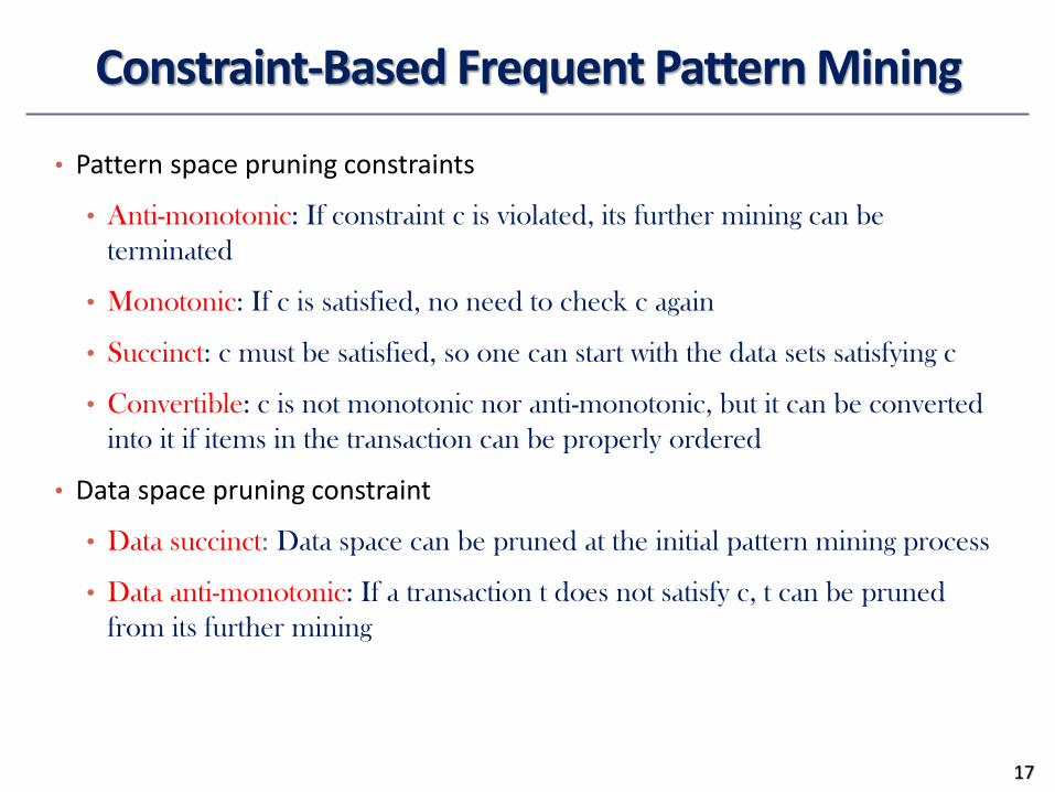
Constraint-Based Frequent Pattern Mining
• Pattern space pruning constraints
• Anti-monotonic: If constraint c is violated, its further mining can be
terminated
• Monotonic: If c is satisfied, no need to check c again
• Succinct: c must be satisfied, so one can start with the data sets satisfying c
• Convertible: c is not monotonic nor anti-monotonic, but it can be converted
into it if items in the transaction can be properly ordered
• Data space pruning constraint
• Data succinct: Data space can be pruned at the initial pattern mining process
• Data anti-monotonic: If a transaction t does not satisfy c, t can be pruned
from its further mining
17
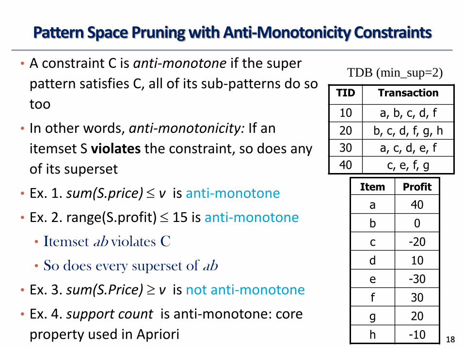
Pattern Space Pruning with Anti-Monotonicity Constraints
• A constraint C is anti-monotone if the super
pattern satisfies C, all of its sub-patterns do so
too
• In other words, anti-monotonicity: If an
itemset S violates the constraint, so does any
of its superset
• Ex. 1. sum(S.price) v is anti-monotone
• Ex. 2. range(S.profit) 15 is anti-monotone
• Itemset ab violates C
• So does every superset of ab
• Ex. 3. sum(S.Price) v is not anti-monotone
• Ex. 4. support count is anti-monotone: core
property used in Apriori
TID Transaction
10 a, b, c, d, f
20 b, c, d, f, g, h
30 a, c, d, e, f
40 c, e, f, g
TDB (min_sup=2)
Item Profit
a 40
b 0
c -20
d 10
e -30
f 30
g 20
h -10 18
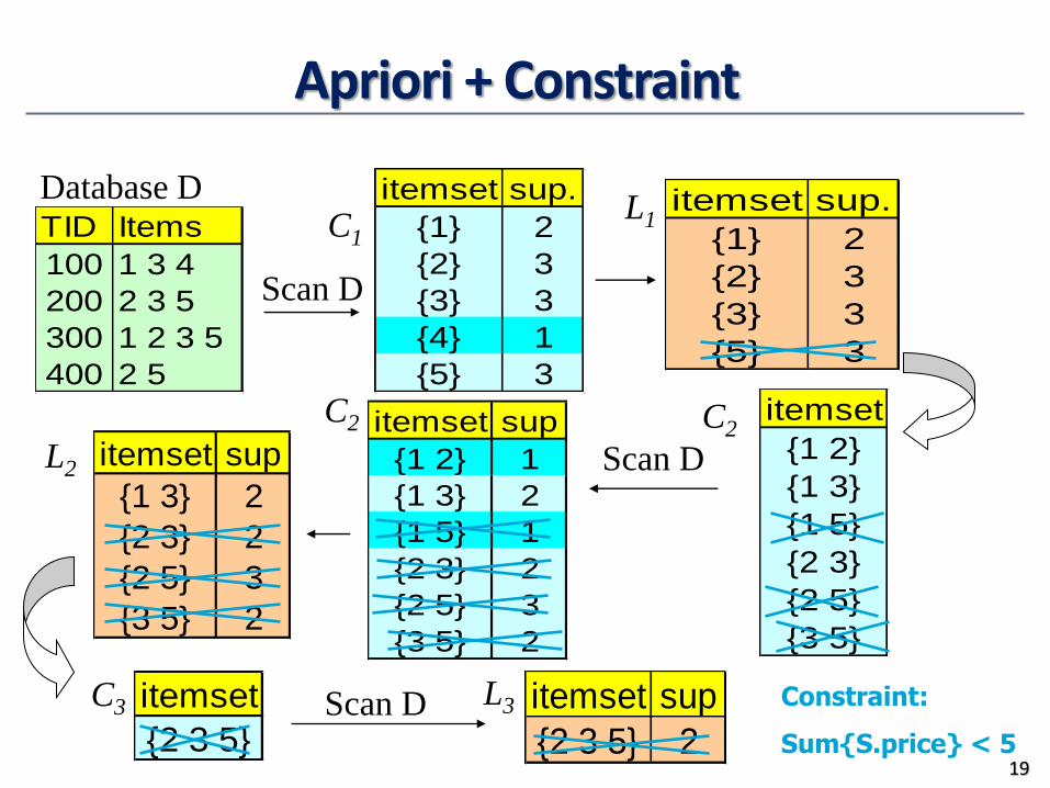
Apriori + Constraint
TID Items
100 1 3 4
200 2 3 5
300 1 2 3 5
400 2 5
Database D itemset sup.
{1} 2
{2} 3
{3} 3
{4} 1
{5} 3
itemset sup.
{1} 2
{2} 3
{3} 3
{5} 3
Scan D
C1
L1
itemset
{1 2}
{1 3}
{1 5}
{2 3}
{2 5}
{3 5}
itemset sup
{1 2} 1
{1 3} 2
{1 5} 1
{2 3} 2
{2 5} 3
{3 5} 2
itemset sup
{1 3} 2
{2 3} 2
{2 5} 3
{3 5} 2
L2
C2 C2
Scan D
C3 L3 itemset
{2 3 5}Scan D itemset sup
{2 3 5} 2
Constraint:
Sum{S.price} < 5 19
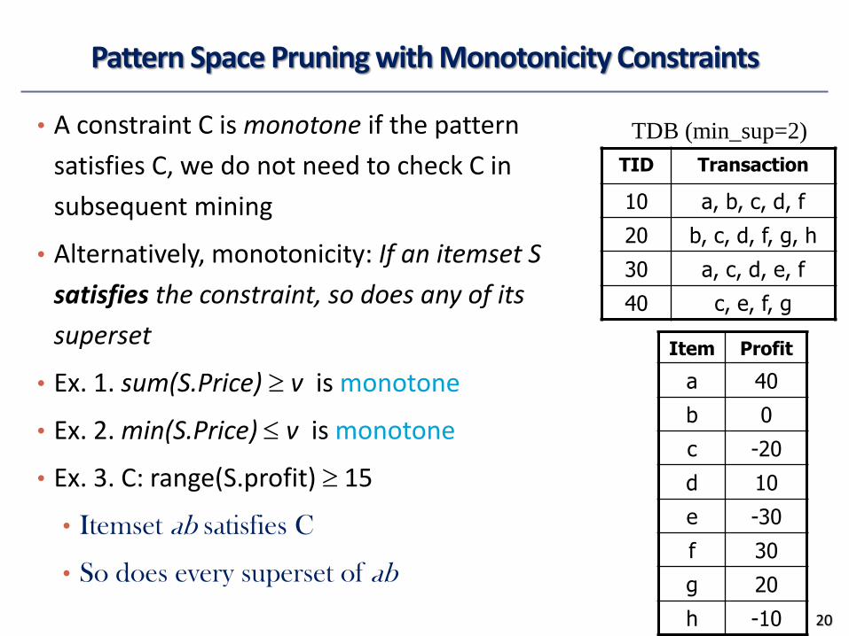
Pattern Space Pruning with Monotonicity Constraints
• A constraint C is monotone if the pattern
satisfies C, we do not need to check C in
subsequent mining
• Alternatively, monotonicity: If an itemset S
satisfies the constraint, so does any of its
superset
• Ex. 1. sum(S.Price) v is monotone
• Ex. 2. min(S.Price) v is monotone
• Ex. 3. C: range(S.profit) 15
• Itemset ab satisfies C
• So does every superset of ab
TID Transaction
10 a, b, c, d, f
20 b, c, d, f, g, h
30 a, c, d, e, f
40 c, e, f, g
TDB (min_sup=2)
Item Profit
a 40
b 0
c -20
d 10
e -30
f 30
g 20
h -10 20
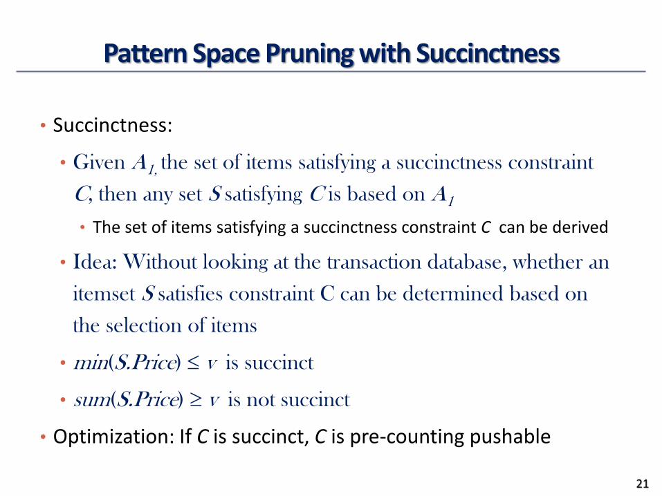
Pattern Space Pruning with Succinctness
• Succinctness:
• Given A1, the set of items satisfying a succinctness constraint
C, then any set S satisfying C is based on A1
• The set of items satisfying a succinctness constraint C can be derived
• Idea: Without looking at the transaction database, whether an
itemset S satisfies constraint C can be determined based on
the selection of items
• min(S.Price) v is succinct
• sum(S.Price) v is not succinct
• Optimization: If C is succinct, C is pre-counting pushable
21
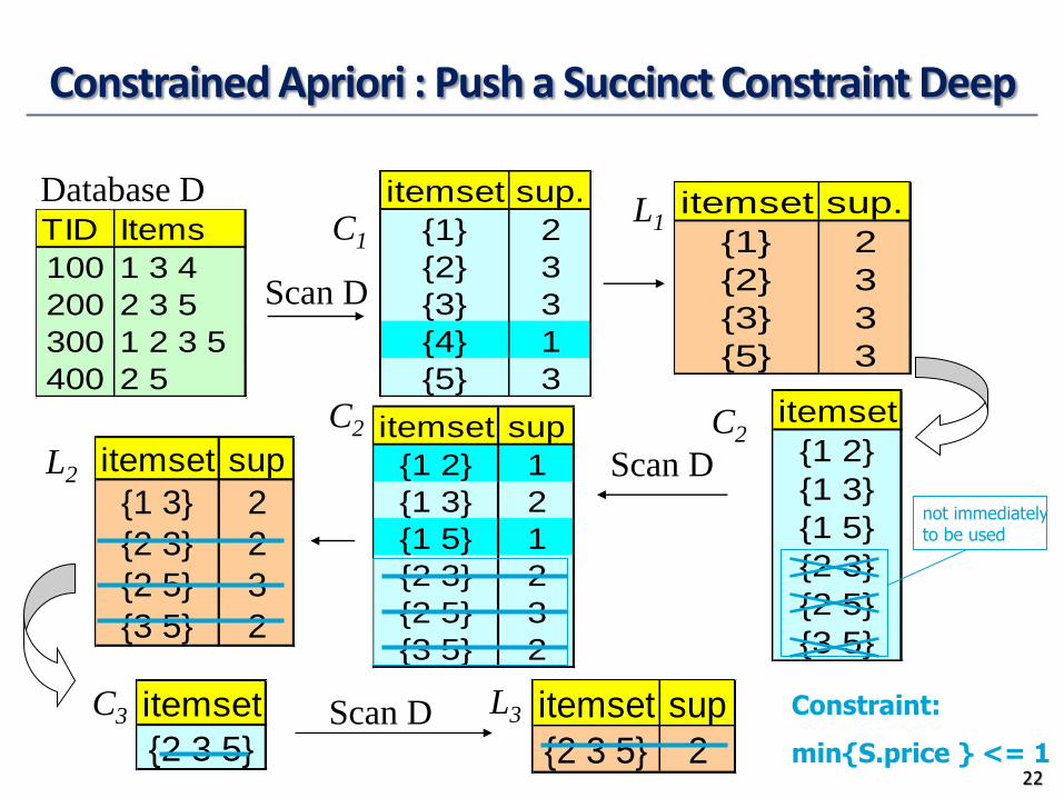
Constrained Apriori : Push a Succinct Constraint Deep
TID Items
100 1 3 4
200 2 3 5
300 1 2 3 5
400 2 5
Database D itemset sup.
{1} 2
{2} 3
{3} 3
{4} 1
{5} 3
itemset sup.
{1} 2
{2} 3
{3} 3
{5} 3
Scan D
C1
L1
itemset
{1 2}
{1 3}
{1 5}
{2 3}
{2 5}
{3 5}
itemset sup
{1 2} 1
{1 3} 2
{1 5} 1
{2 3} 2
{2 5} 3
{3 5} 2
itemset sup
{1 3} 2
{2 3} 2
{2 5} 3
{3 5} 2
L2
C2 C2
Scan D
C3 L3 itemset
{2 3 5}Scan D itemset sup
{2 3 5} 2
Constraint:
min{S.price } <= 1
not immediately to be used
22
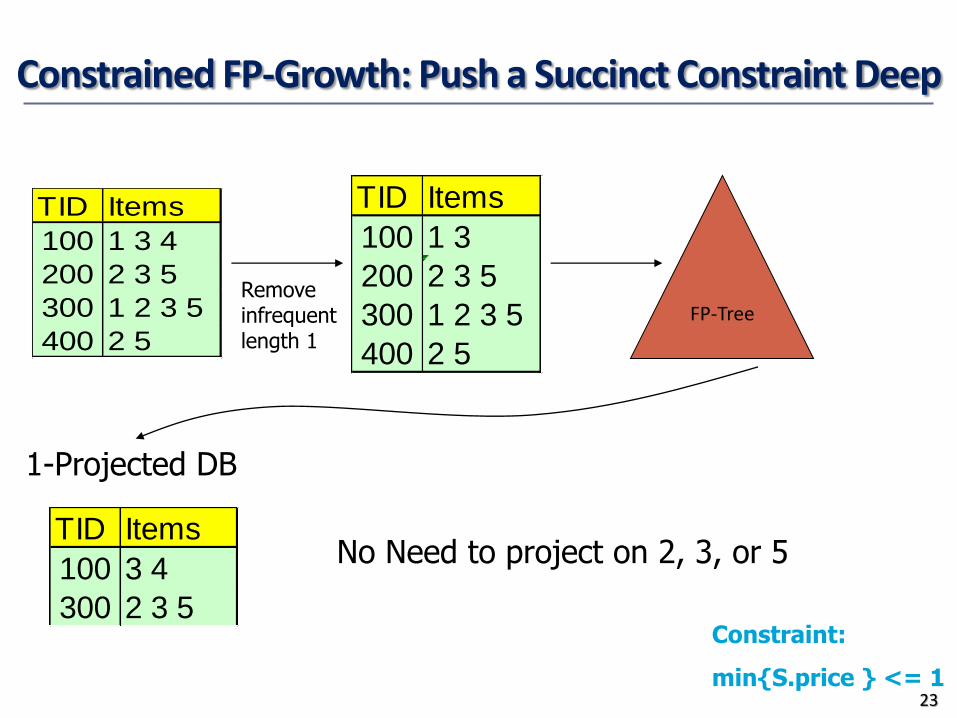
Constrained FP-Growth: Push a Succinct Constraint Deep
Constraint:
min{S.price } <= 1
TID Items
100 1 3 4
200 2 3 5
300 1 2 3 5
400 2 5
TID Items
100 1 3
200 2 3 5
300 1 2 3 5
400 2 5
Remove infrequent length 1
FP-Tree
TID Items
100 3 4
300 2 3 5
1-Projected DB
No Need to project on 2, 3, or 5
23
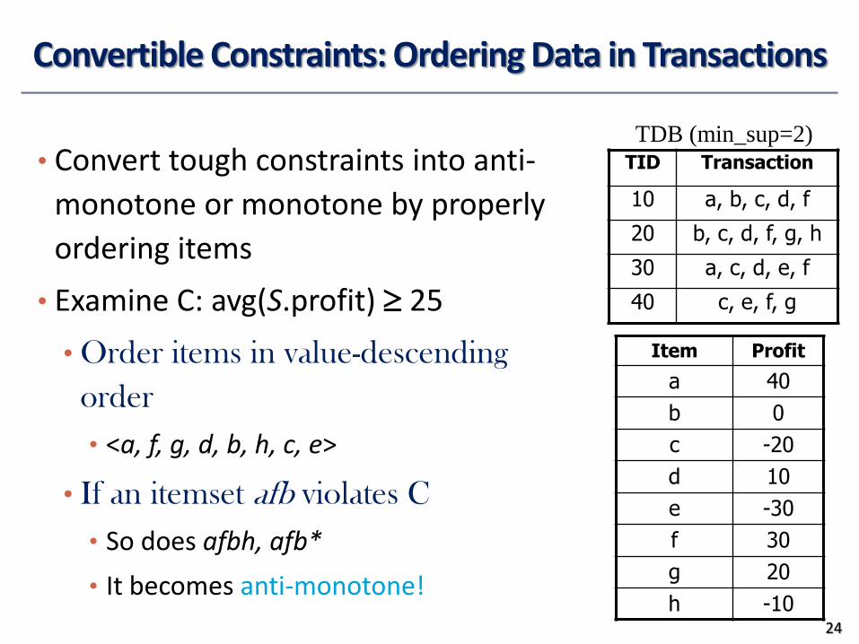
Convertible Constraints: Ordering Data in Transactions
• Convert tough constraints into anti-
monotone or monotone by properly
ordering items
• Examine C: avg(S.profit) 25
• Order items in value-descending
order
• <a, f, g, d, b, h, c, e>
• If an itemset afb violates C
• So does afbh, afb*
• It becomes anti-monotone!
TID Transaction
10 a, b, c, d, f
20 b, c, d, f, g, h
30 a, c, d, e, f
40 c, e, f, g
TDB (min_sup=2)
Item Profit
a 40
b 0
c -20
d 10
e -30
f 30
g 20
h -10 24
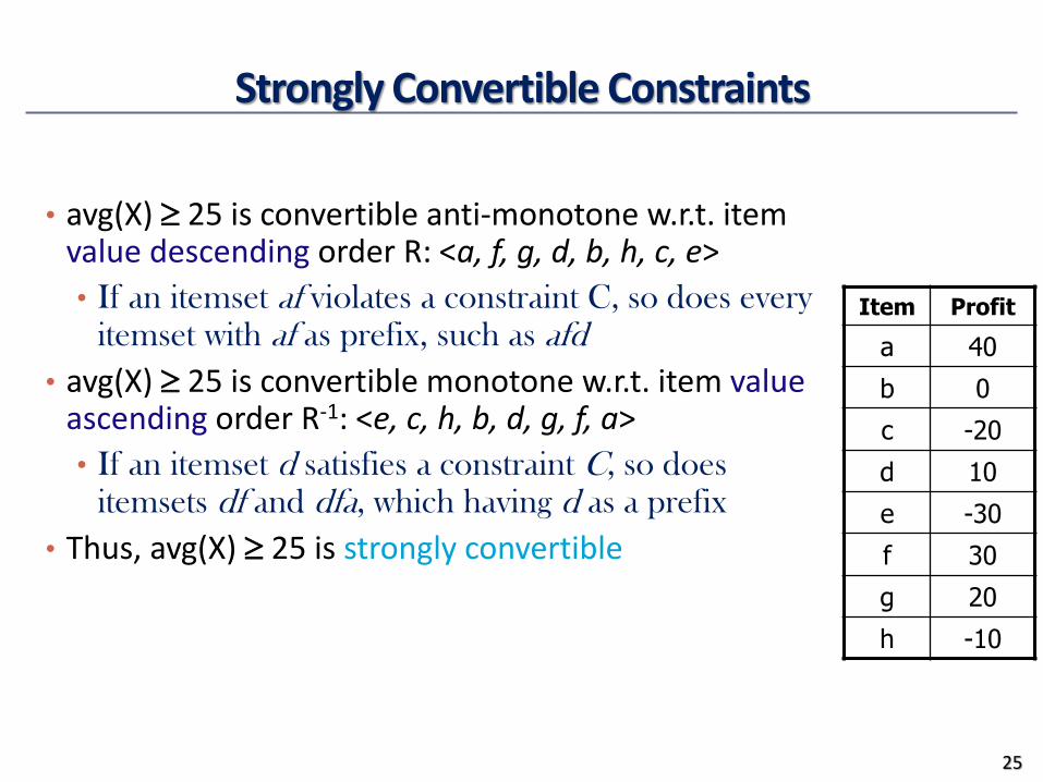
Strongly Convertible Constraints
• avg(X) 25 is convertible anti-monotone w.r.t. item value descending order R: <a, f, g, d, b, h, c, e>
• If an itemset af violates a constraint C, so does every itemset with af as prefix, such as afd
• avg(X) 25 is convertible monotone w.r.t. item value ascending order R-1: <e, c, h, b, d, g, f, a>
• If an itemset d satisfies a constraint C, so does itemsets df and dfa, which having d as a prefix
• Thus, avg(X) 25 is strongly convertible
Item Profit
a 40
b 0
c -20
d 10
e -30
f 30
g 20
h -10
25
Data Space Pruning with Data-Succinct
• Constrains are data-succinct if they can be used at the beginning of a pattern mining process to prune data
• E.g., x ∈ 𝑆, digital camera must be contained in the pattern
26
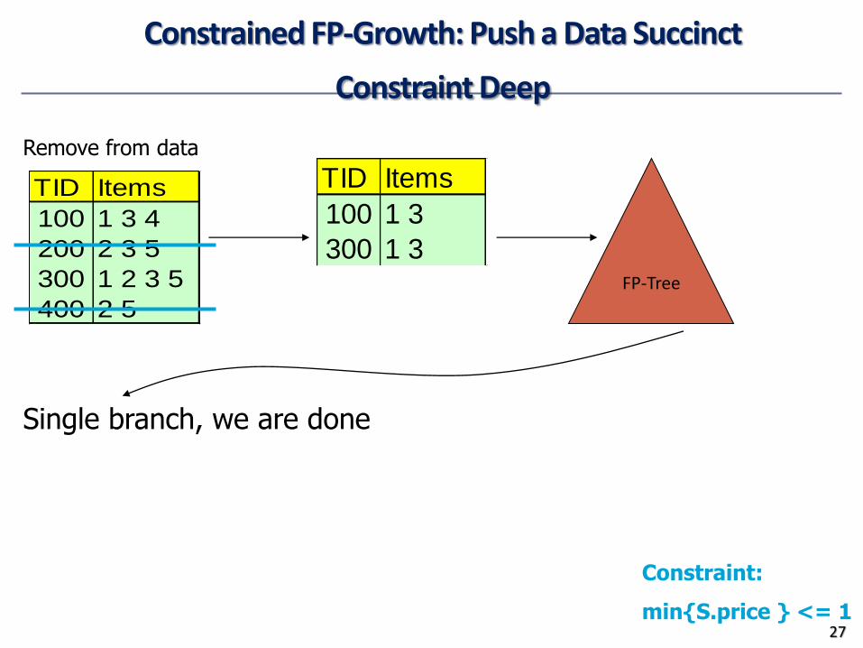
Constrained FP-Growth: Push a Data Succinct
Constraint Deep
Constraint:
min{S.price } <= 1
TID Items
100 1 3 4
200 2 3 5
300 1 2 3 5
400 2 5
TID Items
100 1 3
300 1 3 FP-Tree
Single branch, we are done
Remove from data
27
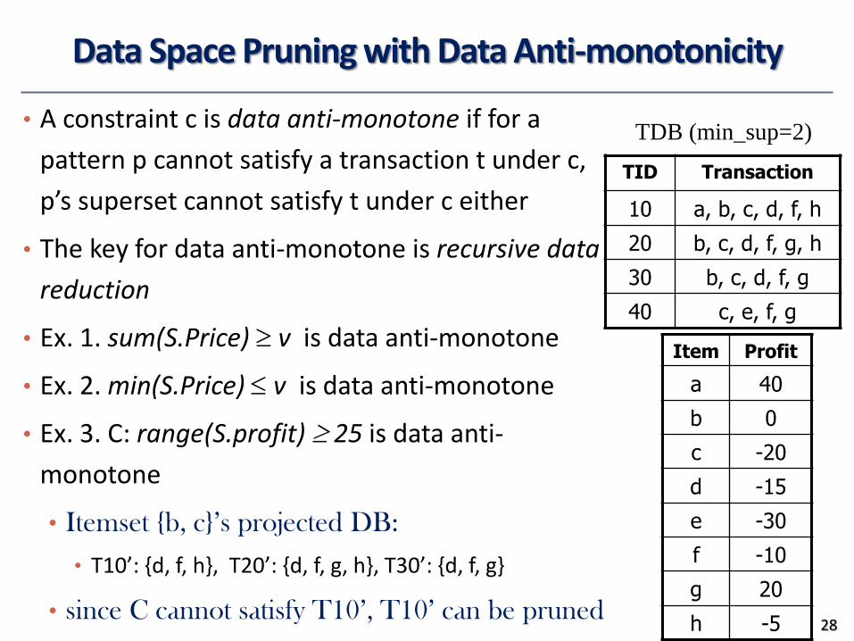
Data Space Pruning with Data Anti-monotonicity
• A constraint c is data anti-monotone if for a
pattern p cannot satisfy a transaction t under c,
p’s superset cannot satisfy t under c either
• The key for data anti-monotone is recursive data
reduction
• Ex. 1. sum(S.Price) v is data anti-monotone
• Ex. 2. min(S.Price) v is data anti-monotone
• Ex. 3. C: range(S.profit) 25 is data anti-
monotone
• Itemset {b, c}’s projected DB:
• T10’: {d, f, h}, T20’: {d, f, g, h}, T30’: {d, f, g}
• since C cannot satisfy T10’, T10’ can be pruned
TID Transaction
10 a, b, c, d, f, h
20 b, c, d, f, g, h
30 b, c, d, f, g
40 c, e, f, g
TDB (min_sup=2)
Item Profit
a 40
b 0
c -20
d -15
e -30
f -10
g 20
h -5 28
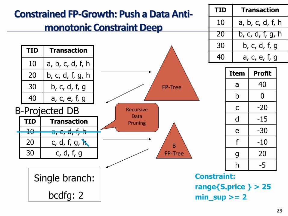
Constrained FP-Growth: Push a Data Anti-monotonic Constraint Deep
Constraint:
range{S.price } > 25
min_sup >= 2
FP-Tree
TID Transaction
10 a, c, d, f, h
20 c, d, f, g, h
30 c, d, f, g
B-Projected DB
B FP-Tree
TID Transaction
10 a, b, c, d, f, h
20 b, c, d, f, g, h
30 b, c, d, f, g
40 a, c, e, f, g
TID Transaction
10 a, b, c, d, f, h
20 b, c, d, f, g, h
30 b, c, d, f, g
40 a, c, e, f, g
Item Profit
a 40
b 0
c -20
d -15
e -30
f -10
g 20
h -5
Recursive Data
Pruning
Single branch:
bcdfg: 2
29
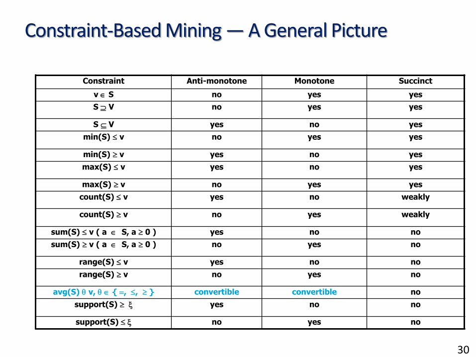
Constraint-Based Mining — A General Picture
Constraint Anti-monotone Monotone Succinct
v S no yes yes
S V no yes yes
S V yes no yes
min(S) v no yes yes
min(S) v yes no yes
max(S) v yes no yes
max(S) v no yes yes
count(S) v yes no weakly
count(S) v no yes weakly
sum(S) v ( a S, a 0 ) yes no no
sum(S) v ( a S, a 0 ) no yes no
range(S) v yes no no
range(S) v no yes no
avg(S) v, { , , } convertible convertible no
support(S) yes no no
support(S) no yes no
30
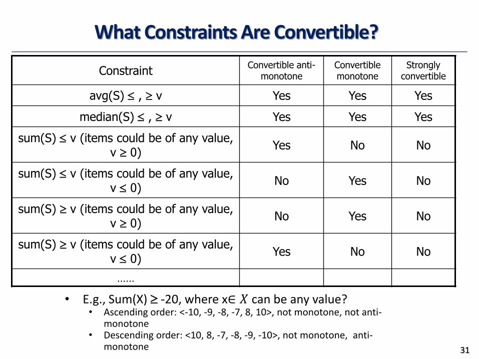
What Constraints Are Convertible?
Constraint Convertible anti-
monotone Convertible monotone
Strongly convertible
avg(S) , v Yes Yes Yes
median(S) , v Yes Yes Yes
sum(S) v (items could be of any value, v 0)
Yes No No
sum(S) v (items could be of any value, v 0)
No Yes No
sum(S) v (items could be of any value, v 0)
No Yes No
sum(S) v (items could be of any value, v 0)
Yes No No
……
31
• E.g., Sum(X) -20, where x∈ 𝑋 can be any value? • Ascending order: <-10, -9, -8, -7, 8, 10>, not monotone, not anti-
monotone • Descending order: <10, 8, -7, -8, -9, -10>, not monotone, anti-
monotone
Chapter 7: Advanced Pattern Mining
• Pattern Mining: A Road Map
• Pattern Mining in Multi-Level, Multi-Dimensional Space
• Constraint-Based Frequent Pattern Mining
• Mining Colossal Patterns
• Mining Compressed or Approximate Patterns
• Summary
32
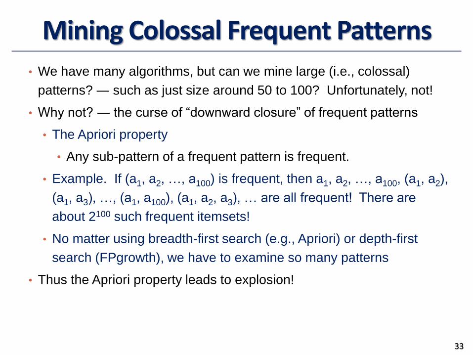
Mining Colossal Frequent Patterns
• We have many algorithms, but can we mine large (i.e., colossal)
patterns? ― such as just size around 50 to 100? Unfortunately, not!
• Why not? ― the curse of “downward closure” of frequent patterns
• The Apriori property
• Any sub-pattern of a frequent pattern is frequent.
• Example. If (a1, a2, …, a100) is frequent, then a1, a2, …, a100, (a1, a2),
(a1, a3), …, (a1, a100), (a1, a2, a3), … are all frequent! There are
about 2100 such frequent itemsets!
• No matter using breadth-first search (e.g., Apriori) or depth-first
search (FPgrowth), we have to examine so many patterns
• Thus the Apriori property leads to explosion!
33
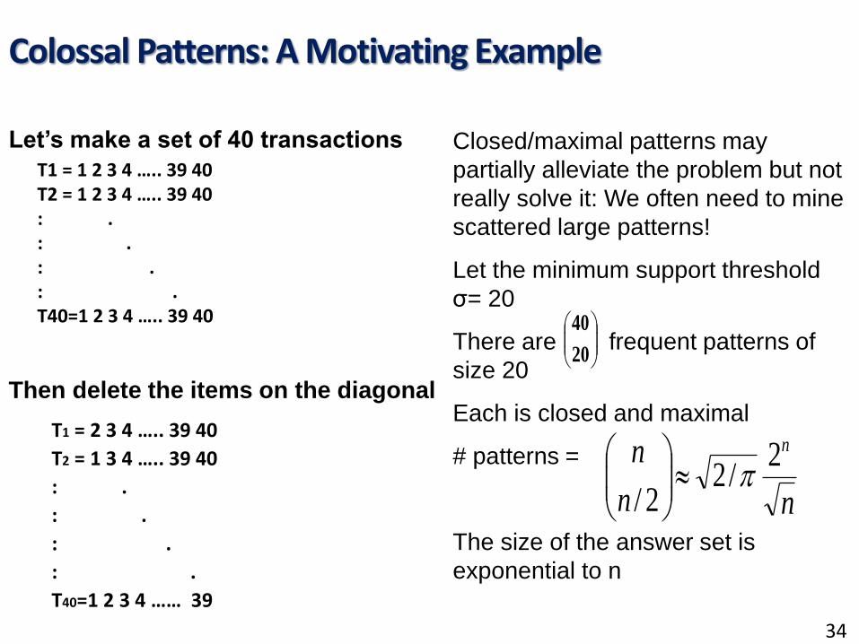
Closed/maximal patterns may
partially alleviate the problem but not
really solve it: We often need to mine
scattered large patterns!
Let the minimum support threshold
σ= 20
There are frequent patterns of
size 20
Each is closed and maximal
# patterns =
The size of the answer set is
exponential to n
Colossal Patterns: A Motivating Example
T1 = 1 2 3 4 ….. 39 40 T2 = 1 2 3 4 ….. 39 40 : . : . : . : . T40=1 2 3 4 ….. 39 40
20
40
T1 = 2 3 4 ….. 39 40
T2 = 1 3 4 ….. 39 40
: .
: .
: .
: .
T40=1 2 3 4 …… 39
nn
n n2/2
2/
Then delete the items on the diagonal
Let’s make a set of 40 transactions
34
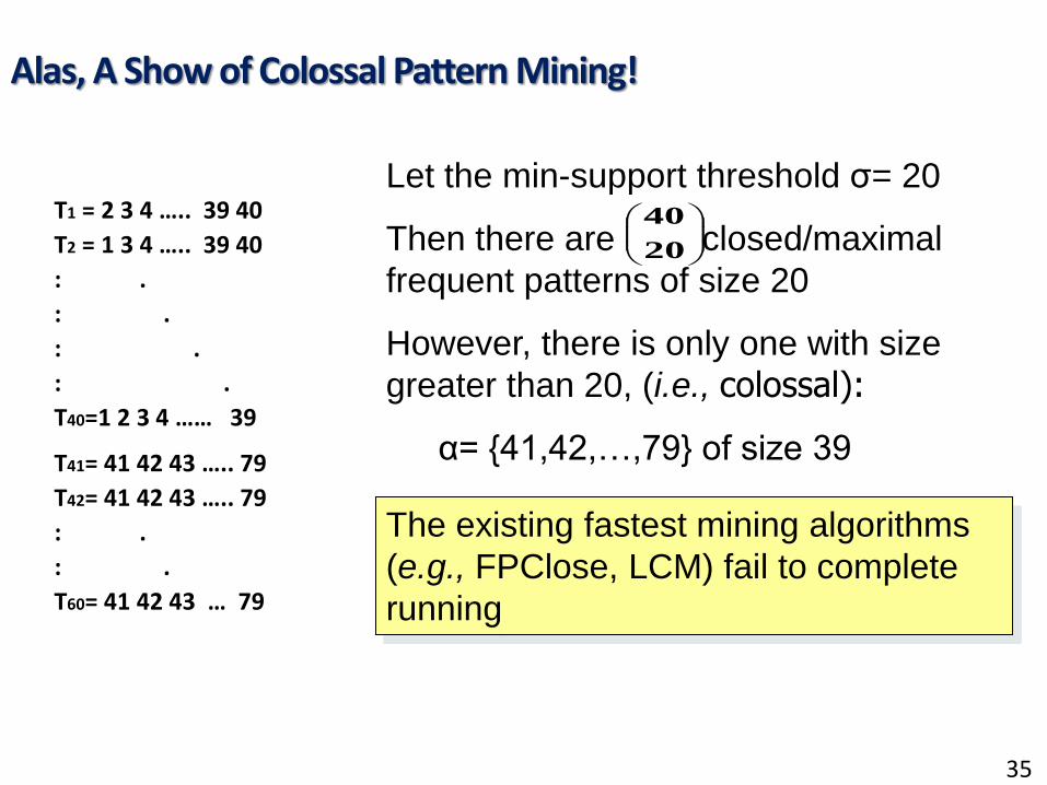
Let the min-support threshold σ= 20
Then there are closed/maximal
frequent patterns of size 20
However, there is only one with size
greater than 20, (i.e., colossal):
α= {41,42,…,79} of size 39
Alas, A Show of Colossal Pattern Mining!
20
40T1 = 2 3 4 ….. 39 40
T2 = 1 3 4 ….. 39 40
: .
: .
: .
: .
T40=1 2 3 4 …… 39
T41= 41 42 43 ….. 79
T42= 41 42 43 ….. 79
: .
: .
T60= 41 42 43 … 79
The existing fastest mining algorithms
(e.g., FPClose, LCM) fail to complete
running
35
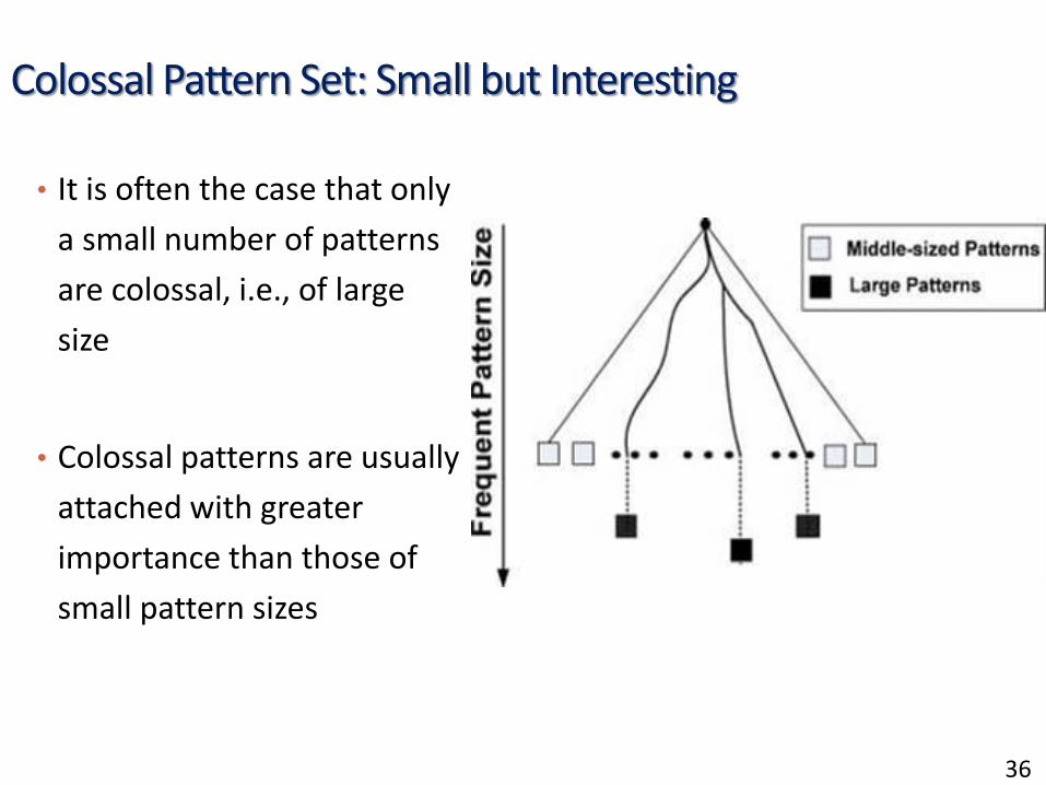
Colossal Pattern Set: Small but Interesting
• It is often the case that only
a small number of patterns
are colossal, i.e., of large
size
• Colossal patterns are usually
attached with greater
importance than those of
small pattern sizes
36
Mining Colossal Patterns: Motivation and Philosophy
• Motivation: Many real-world tasks need mining colossal patterns
• Micro-array analysis in bioinformatics (when support is low)
• Biological sequence patterns
• Biological/sociological/information graph pattern mining
• No hope for completeness
• If the mining of mid-sized patterns is explosive in size, there is no hope to find colossal patterns efficiently by insisting “complete set” mining philosophy
• Jumping out of the swamp of the mid-sized results
• What we may develop is a philosophy that may jump out of the swamp of mid-sized results that are explosive in size and jump to reach colossal patterns
• Striving for mining almost complete colossal patterns
• The key is to develop a mechanism that may quickly reach colossal patterns and discover most of them
37
Methodology of Pattern-Fusion Strategy
• Pattern-Fusion traverses the tree in a bounded-breadth way
• Always pushes down a frontier of a bounded-size candidate pool
• Only a fixed number of patterns in the current candidate pool will
be used as the starting nodes to go down in the pattern tree ―
thus avoids the exponential search space
• Pattern-Fusion identifies “shortcuts” whenever possible
• Pattern growth is not performed by single-item addition but by
leaps and bounded: agglomeration of multiple patterns in the pool
• These shortcuts will direct the search down the tree much more
rapidly towards the colossal patterns
38
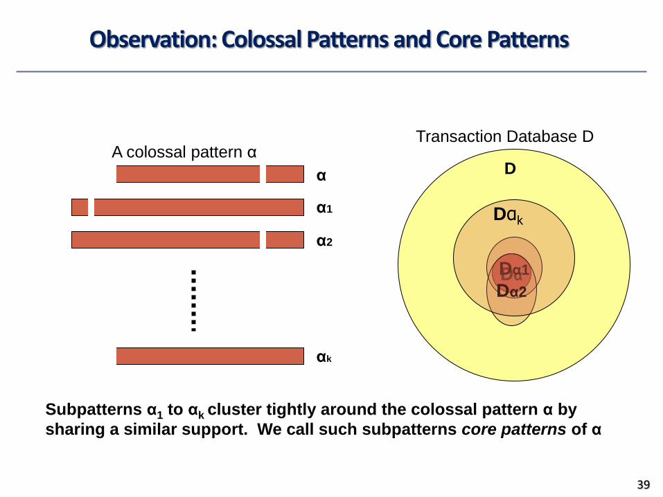
Observation: Colossal Patterns and Core Patterns
A colossal pattern α D
Dα
α1
Transaction Database D
Dα1
Dα2
α2
α
αk
Dαk
Subpatterns α1 to αk cluster tightly around the colossal pattern α by
sharing a similar support. We call such subpatterns core patterns of α
39
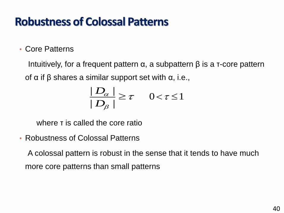
Robustness of Colossal Patterns
• Core Patterns
Intuitively, for a frequent pattern α, a subpattern β is a τ-core pattern
of α if β shares a similar support set with α, i.e.,
where τ is called the core ratio
• Robustness of Colossal Patterns
A colossal pattern is robust in the sense that it tends to have much
more core patterns than small patterns
||
||
D
D10
40
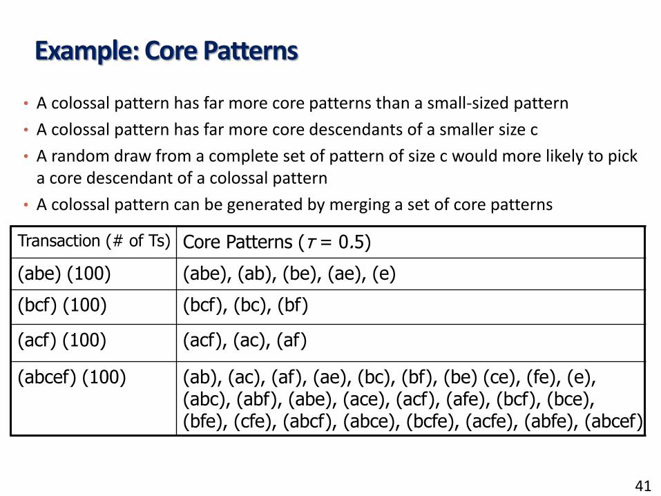
Example: Core Patterns
• A colossal pattern has far more core patterns than a small-sized pattern
• A colossal pattern has far more core descendants of a smaller size c
• A random draw from a complete set of pattern of size c would more likely to pick a core descendant of a colossal pattern
• A colossal pattern can be generated by merging a set of core patterns
Transaction (# of Ts) Core Patterns (τ = 0.5)
(abe) (100) (abe), (ab), (be), (ae), (e)
(bcf) (100) (bcf), (bc), (bf)
(acf) (100) (acf), (ac), (af)
(abcef) (100) (ab), (ac), (af), (ae), (bc), (bf), (be) (ce), (fe), (e), (abc), (abf), (abe), (ace), (acf), (afe), (bcf), (bce), (bfe), (cfe), (abcf), (abce), (bcfe), (acfe), (abfe), (abcef)
41
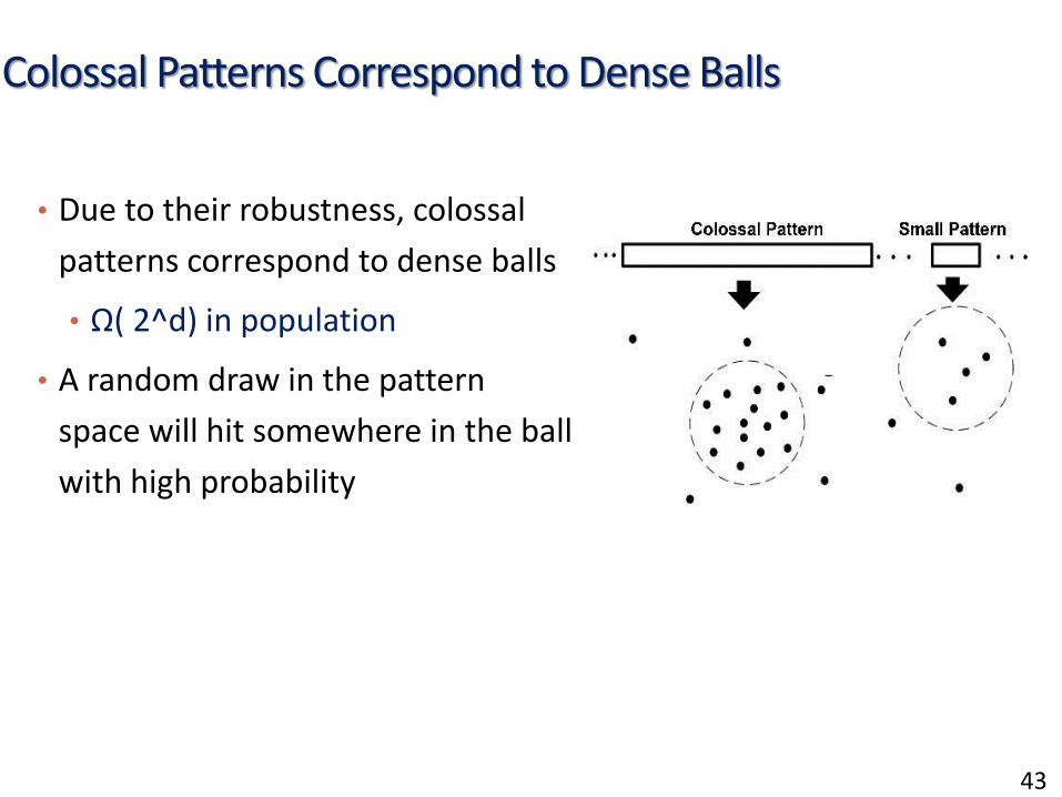
Colossal Patterns Correspond to Dense Balls
• Due to their robustness, colossal
patterns correspond to dense balls
• Ω( 2^d) in population
• A random draw in the pattern
space will hit somewhere in the ball
with high probability
43
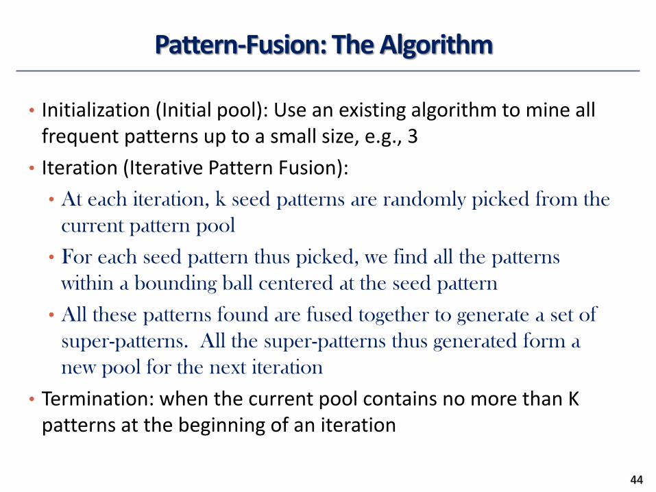
Pattern-Fusion: The Algorithm
• Initialization (Initial pool): Use an existing algorithm to mine all frequent patterns up to a small size, e.g., 3
• Iteration (Iterative Pattern Fusion):
• At each iteration, k seed patterns are randomly picked from the
current pattern pool
• For each seed pattern thus picked, we find all the patterns
within a bounding ball centered at the seed pattern
• All these patterns found are fused together to generate a set of
super-patterns. All the super-patterns thus generated form a
new pool for the next iteration
• Termination: when the current pool contains no more than K patterns at the beginning of an iteration
44
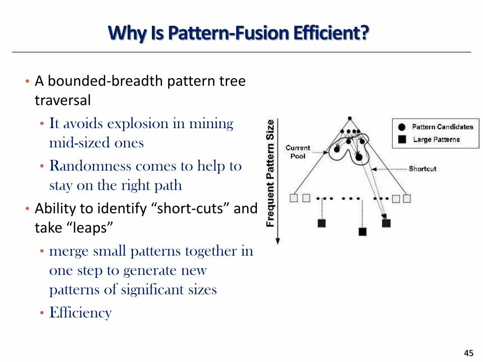
Why Is Pattern-Fusion Efficient?
• A bounded-breadth pattern tree traversal
• It avoids explosion in mining
mid-sized ones
• Randomness comes to help to
stay on the right path
• Ability to identify “short-cuts” and take “leaps”
• merge small patterns together in
one step to generate new
patterns of significant sizes
• Efficiency
45
Pattern-Fusion Leads to Good Approximation
• Gearing toward colossal patterns
• The larger the pattern, the greater the chance it will be
generated
• Catching outliers
• The more distinct the pattern, the greater the chance it will be
generated
46
Chapter 7: Advanced Pattern Mining
• Pattern Mining: A Road Map
• Pattern Mining in Multi-Level, Multi-Dimensional Space
• Constraint-Based Frequent Pattern Mining
• Mining Colossal Patterns
• Mining Compressed or Approximate Patterns
• Summary
47
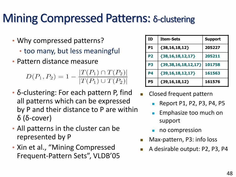
Mining Compressed Patterns: δ-clustering
• Why compressed patterns?
• too many, but less meaningful
• Pattern distance measure
• δ-clustering: For each pattern P, find all patterns which can be expressed by P and their distance to P are within δ (δ-cover)
• All patterns in the cluster can be represented by P
• Xin et al., “Mining Compressed Frequent-Pattern Sets”, VLDB’05
ID Item-Sets Support
P1 {38,16,18,12} 205227
P2 {38,16,18,12,17} 205211
P3 {39,38,16,18,12,17} 101758
P4 {39,16,18,12,17} 161563
P5 {39,16,18,12} 161576
Closed frequent pattern
Report P1, P2, P3, P4, P5
Emphasize too much on support
no compression
Max-pattern, P3: info loss
A desirable output: P2, P3, P4
48
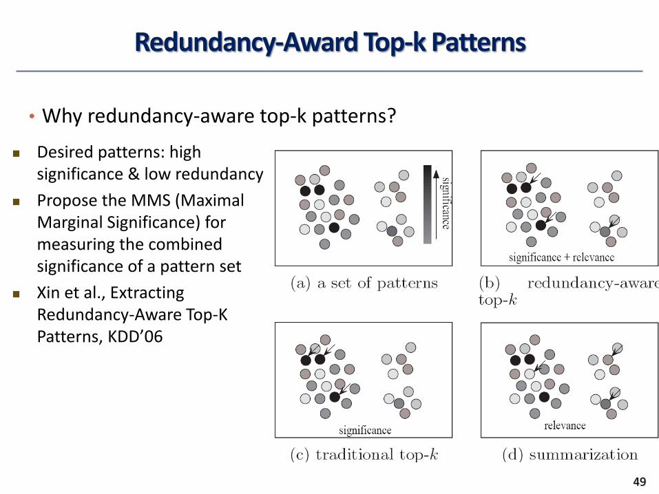
Redundancy-Award Top-k Patterns
• Why redundancy-aware top-k patterns?
Desired patterns: high significance & low redundancy
Propose the MMS (Maximal Marginal Significance) for measuring the combined significance of a pattern set
Xin et al., Extracting Redundancy-Aware Top-K Patterns, KDD’06
49
Chapter 7: Advanced Pattern Mining
• Pattern Mining: A Road Map
• Pattern Mining in Multi-Level, Multi-Dimensional Space
• Constraint-Based Frequent Pattern Mining
• Mining Colossal Patterns
• Mining Compressed or Approximate Patterns
• Summary
50
Summary
• Roadmap: Many aspects & extensions on pattern mining
• Mining patterns in multi-level, multi dimensional space,
Mining rare and negative patterns
• Constraint-based pattern mining
• Specialized methods for mining colossal patterns
• Mining compressed or approximate patterns
51
52
Ref: Mining Multi-Level and Quantitative Rules
• R. Srikant and R. Agrawal. Mining generalized association rules. VLDB'95.
• J. Han and Y. Fu. Discovery of multiple-level association rules from large databases. VLDB'95.
• R. Srikant and R. Agrawal. Mining quantitative association rules in large relational tables. SIGMOD'96.
• T. Fukuda, Y. Morimoto, S. Morishita, and T. Tokuyama. Data mining using two-dimensional optimized association rules: Scheme, algorithms, and visualization. SIGMOD'96.
• K. Yoda, T. Fukuda, Y. Morimoto, S. Morishita, and T. Tokuyama. Computing optimized rectilinear regions for association rules. KDD'97.
• R.J. Miller and Y. Yang. Association rules over interval data. SIGMOD'97.
• Y. Aumann and Y. Lindell. A Statistical Theory for Quantitative Association Rules KDD'99.
53
Ref: Mining Other Kinds of Rules
• R. Meo, G. Psaila, and S. Ceri. A new SQL-like operator for mining association
rules. VLDB'96.
• B. Lent, A. Swami, and J. Widom. Clustering association rules. ICDE'97.
• A. Savasere, E. Omiecinski, and S. Navathe. Mining for strong negative
associations in a large database of customer transactions. ICDE'98.
• D. Tsur, J. D. Ullman, S. Abitboul, C. Clifton, R. Motwani, and S. Nestorov.
Query flocks: A generalization of association-rule mining. SIGMOD'98.
• F. Korn, A. Labrinidis, Y. Kotidis, and C. Faloutsos. Ratio rules: A new
paradigm for fast, quantifiable data mining. VLDB'98.
• F. Zhu, X. Yan, J. Han, P. S. Yu, and H. Cheng, “Mining Colossal Frequent
Patterns by Core Pattern Fusion”, ICDE'07.
54
Ref: Constraint-Based Pattern Mining
• R. Srikant, Q. Vu, and R. Agrawal. Mining association rules with item
constraints. KDD'97
• R. Ng, L.V.S. Lakshmanan, J. Han & A. Pang. Exploratory mining and pruning
optimizations of constrained association rules. SIGMOD’98
• G. Grahne, L. Lakshmanan, and X. Wang. Efficient mining of constrained
correlated sets. ICDE'00
• J. Pei, J. Han, and L. V. S. Lakshmanan. Mining Frequent Itemsets with
Convertible Constraints. ICDE'01
• J. Pei, J. Han, and W. Wang, Mining Sequential Patterns with Constraints in
Large Databases, CIKM'02
• F. Bonchi, F. Giannotti, A. Mazzanti, and D. Pedreschi. ExAnte: Anticipated
Data Reduction in Constrained Pattern Mining, PKDD'03
• F. Zhu, X. Yan, J. Han, and P. S. Yu, “gPrune: A Constraint Pushing Framework
for Graph Pattern Mining”, PAKDD'07
55
Ref: Mining Sequential and Structured Patterns
• R. Srikant and R. Agrawal. Mining sequential patterns: Generalizations and
performance improvements. EDBT’96.
• H. Mannila, H Toivonen, and A. I. Verkamo. Discovery of frequent episodes in
event sequences. DAMI:97.
• M. Zaki. SPADE: An Efficient Algorithm for Mining Frequent Sequences. Machine
Learning:01.
• J. Pei, J. Han, H. Pinto, Q. Chen, U. Dayal, and M.-C. Hsu. PrefixSpan: Mining
Sequential Patterns Efficiently by Prefix-Projected Pattern Growth. ICDE'01.
• M. Kuramochi and G. Karypis. Frequent Subgraph Discovery. ICDM'01.
• X. Yan, J. Han, and R. Afshar. CloSpan: Mining Closed Sequential Patterns in
Large Datasets. SDM'03.
• X. Yan and J. Han. CloseGraph: Mining Closed Frequent Graph Patterns.
KDD'03.
56
Ref: Mining Spatial, Multimedia, and Web Data
• K. Koperski and J. Han, Discovery of Spatial Association Rules in Geographic
Information Databases, SSD’95.
• O. R. Zaiane, M. Xin, J. Han, Discovering Web Access Patterns and Trends by
Applying OLAP and Data Mining Technology on Web Logs. ADL'98.
• O. R. Zaiane, J. Han, and H. Zhu, Mining Recurrent Items in Multimedia with
Progressive Resolution Refinement. ICDE'00.
• D. Gunopulos and I. Tsoukatos. Efficient Mining of Spatiotemporal Patterns.
SSTD'01.
57
Ref: Mining Frequent Patterns in Time-Series Data
• B. Ozden, S. Ramaswamy, and A. Silberschatz. Cyclic association rules. ICDE'98.
• J. Han, G. Dong and Y. Yin, Efficient Mining of Partial Periodic Patterns in Time
Series Database, ICDE'99.
• H. Lu, L. Feng, and J. Han. Beyond Intra-Transaction Association Analysis:
Mining Multi-Dimensional Inter-Transaction Association Rules. TOIS:00.
• B.-K. Yi, N. Sidiropoulos, T. Johnson, H. V. Jagadish, C. Faloutsos, and A. Biliris.
Online Data Mining for Co-Evolving Time Sequences. ICDE'00.
• W. Wang, J. Yang, R. Muntz. TAR: Temporal Association Rules on Evolving
Numerical Attributes. ICDE’01.
• J. Yang, W. Wang, P. S. Yu. Mining Asynchronous Periodic Patterns in Time Series
Data. TKDE’03.
58
Ref: FP for Classification and Clustering
• G. Dong and J. Li. Efficient mining of emerging patterns: Discovering
trends and differences. KDD'99.
• B. Liu, W. Hsu, Y. Ma. Integrating Classification and Association Rule
Mining. KDD’98.
• W. Li, J. Han, and J. Pei. CMAR: Accurate and Efficient Classification Based
on Multiple Class-Association Rules. ICDM'01.
• H. Wang, W. Wang, J. Yang, and P.S. Yu. Clustering by pattern similarity in
large data sets. SIGMOD’ 02.
• J. Yang and W. Wang. CLUSEQ: efficient and effective sequence clustering.
ICDE’03.
• X. Yin and J. Han. CPAR: Classification based on Predictive Association
Rules. SDM'03.
• H. Cheng, X. Yan, J. Han, and C.-W. Hsu, Discriminative Frequent Pattern
Analysis for Effective Classification”, ICDE'07.
59
Ref: Stream and Privacy-Preserving FP Mining
• A. Evfimievski, R. Srikant, R. Agrawal, J. Gehrke. Privacy Preserving Mining
of Association Rules. KDD’02.
• J. Vaidya and C. Clifton. Privacy Preserving Association Rule Mining in
Vertically Partitioned Data. KDD’02.
• G. Manku and R. Motwani. Approximate Frequency Counts over Data
Streams. VLDB’02.
• Y. Chen, G. Dong, J. Han, B. W. Wah, and J. Wang. Multi-Dimensional
Regression Analysis of Time-Series Data Streams. VLDB'02.
• C. Giannella, J. Han, J. Pei, X. Yan and P. S. Yu. Mining Frequent Patterns in
Data Streams at Multiple Time Granularities, Next Generation Data
Mining:03.
• A. Evfimievski, J. Gehrke, and R. Srikant. Limiting Privacy Breaches in
Privacy Preserving Data Mining. PODS’03.
60
Ref: Other Freq. Pattern Mining Applications
• Y. Huhtala, J. Kärkkäinen, P. Porkka, H. Toivonen. Efficient Discovery of
Functional and Approximate Dependencies Using Partitions. ICDE’98.
• H. V. Jagadish, J. Madar, and R. Ng. Semantic Compression and Pattern
Extraction with Fascicles. VLDB'99.
• T. Dasu, T. Johnson, S. Muthukrishnan, and V. Shkapenyuk. Mining
Database Structure; or How to Build a Data Quality Browser. SIGMOD'02.
• K. Wang, S. Zhou, J. Han. Profit Mining: From Patterns to Actions.
EDBT’02.
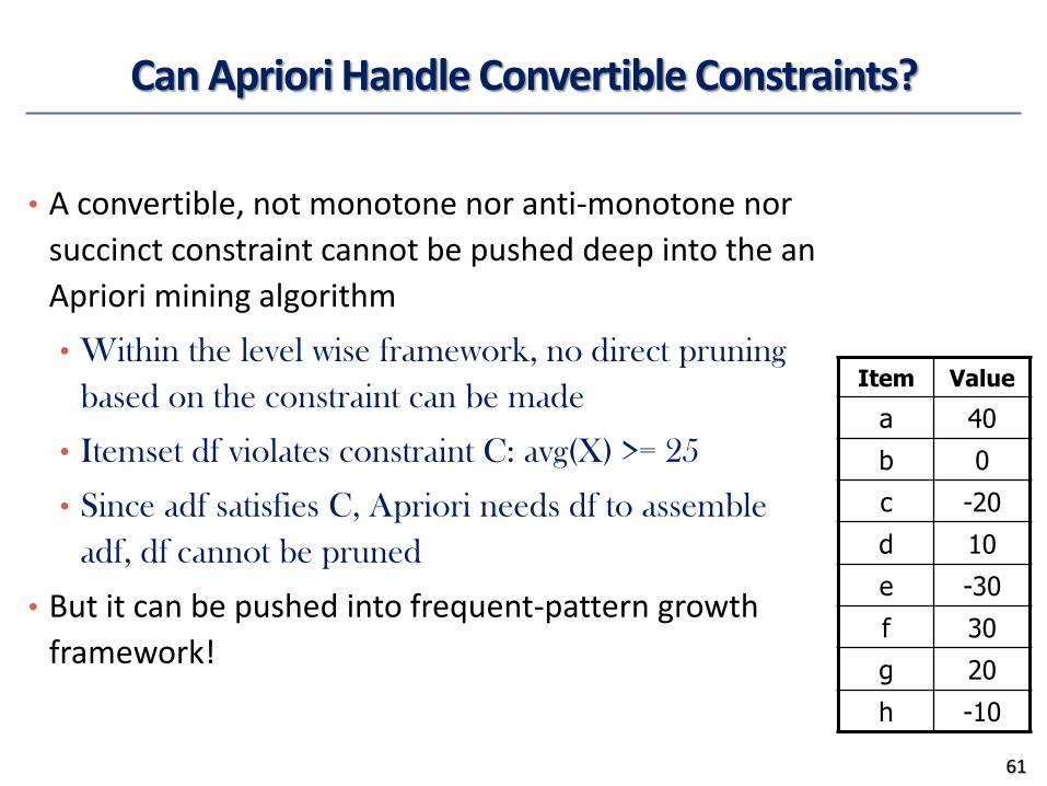
Can Apriori Handle Convertible Constraints?
• A convertible, not monotone nor anti-monotone nor
succinct constraint cannot be pushed deep into the an
Apriori mining algorithm
• Within the level wise framework, no direct pruning
based on the constraint can be made
• Itemset df violates constraint C: avg(X) >= 25
• Since adf satisfies C, Apriori needs df to assemble
adf, df cannot be pruned
• But it can be pushed into frequent-pattern growth
framework!
Item Value
a 40
b 0
c -20
d 10
e -30
f 30
g 20
h -10
61
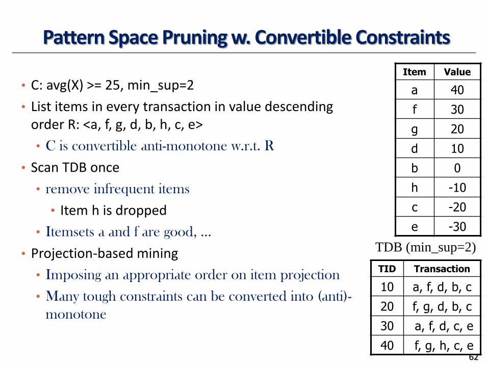
Pattern Space Pruning w. Convertible Constraints
• C: avg(X) >= 25, min_sup=2
• List items in every transaction in value descending order R: <a, f, g, d, b, h, c, e>
• C is convertible anti-monotone w.r.t. R
• Scan TDB once
• remove infrequent items
• Item h is dropped
• Itemsets a and f are good, …
• Projection-based mining
• Imposing an appropriate order on item projection
• Many tough constraints can be converted into (anti)-
monotone
TID Transaction
10 a, f, d, b, c
20 f, g, d, b, c
30 a, f, d, c, e
40 f, g, h, c, e
TDB (min_sup=2)
Item Value
a 40
f 30
g 20
d 10
b 0
h -10
c -20
e -30
62
Handling Multiple Constraints
• Different constraints may require different or even conflicting
item-ordering
• If there exists an order R s.t. both C1 and C2 are convertible
w.r.t. R, then there is no conflict between the two convertible
constraints
• If there exists conflict on order of items
• Try to satisfy one constraint first
• Then using the order for the other constraint to mine
frequent itemsets in the corresponding projected database
63