CS464 Introduction to Machine Learning1 Decision Tree Learning Decision tree learning is a method...

CS464 Introduction to Machine Learning 1

Decision Tree Learning

• Decision tree learning is a method for approximating discrete-valued target functions.

• The learned function is represented by a decision tree.– A learned decision tree can also be re-represented as a set of if-then rules.

• Decision tree learning is one of the most widely used and practical methods for inductive inference.

• It is robust to noisy data and capable of learning disjunctive expressions.

• Decision tree learning method searches a completely expressive hypothesis .– Avoids the difficulties of restricted hypothesis spaces. – Its inductive bias is a preference for small trees over large trees.

• The decision tree algorithms such as ID3, C4.5 are very popular inductive inference algorithms, and they are sucessfully applied to many leaning tasks.



Decision Tree for PlayTennis


Outlook

Sunny Overcast Rain

Humidity

High Normal

Wind

Strong Weak

No Yes

Yes

YesNo


Decision Tree

• Decision trees represent a disjunction of conjunctions of constraints on the attribute values of instances.

• Each path from the tree root to a leaf corresponds to a conjunction of attribute tests, and

• The tree itself is a disjunction of these conjunctions.

(Outlook = Sunny Humidity = Normal) (Outlook = Overcast) (Outlook = Rain Wind = Weak)

Outlook

Sunny Overcast Rain

Humidity

High Normal

Wind

Strong Weak

No Yes

Yes

YesNo


Decision Tree

• Decision trees classify instances by sorting them down the tree from the root to some leaf node, which provides the classification of the instance.

• Each node in the tree specifies a test of some attribute of the instance.

• Each branch descending from a node corresponds to one of the possible values for the attribute.

• Each leaf node assigns a classification.

• The instance

(Outlook=Sunny, Temperature=Hot, Humidity=High, Wind=Strong)

is classified as a negative instance.



When to Consider Decision Trees

• Instances are represented by attribute-value pairs.– Fixed set of attributes, and the attributes take a small number of disjoint possible values.

• The target function has discrete output values.– Decision tree learning is appropriate for a boolean classification, but it easily extends to learning

functions with more than two possible output values.

• Disjunctive descriptions may be required.– decision trees naturally represent disjunctive expressions.

• The training data may contain errors.– Decision tree learning methods are robust to errors, both errors in classifications of the training

examples and errors in the attribute values that describe these examples.

• The training data may contain missing attribute values.– Decision tree methods can be used even when some training examples have unknown values.

• Decision tree learning has been applied to problems such as learning to classify– medical patients by their disease,

– equipment malfunctions by their cause, and

– loan applicants by their likelihood of defaulting on payments.


Top-Down Induction of Decision Trees -- ID3

1. A the “best” decision attribute for next node

2. Assign A as decision attribute for node

3. For each value of A create new descendant node

4. Sort training examples to leaf node according to the attribute value of the branch

5. If all training examples are perfectly classified (same value of target attribute) STOP,

else iterate over new leaf nodes.


Which Attribute is ”best”?

• We would like to select the attribute that is most useful for classifying examples.

• Informution gain measures how well a given attribute separates the training examples according to their target classification.

• ID3 uses this information gain measure to select among the candidate attributes at each step while growing the tree.

• In order to define information gain precisely, we use a measure commonly used in information theory, called entropy

• Entropy characterizes the (im)purity of an arbitrary collection of examples.


Which Attribute is ”best”?

A1=?

True False

[21+, 5-] [8+, 30-]

[29+,35-] A2=?

True False

[18+, 33-] [11+, 2-]

[29+,35-]


Entropy

• Given a collection S, containing positive and negative examples of some target concept, the entropy of S relative to this boolean classification is:

Entropy(S) = -p+ log2p+ - p- log2p-

• S is a sample of training examples

• p+ is the proportion of positive examples

• p- is the proportion of negative examples


Entropy


Entropy

Entropy([9+,5-] = – (9/14) log2(9/14) – (5/14) log2(5/14) = 0.940

Entropy([12+,4-] = – (12/16) log2(12/16) – (4/16) log2(4/16) = 0.811

Entropy([12+,5-] = – (12/17) log2(12/17) – (5/17) log2(5/17) = 0.874

Entropy([8+,8-] = – (8/16) log2(8/16) – (8/16) log2(8/16) = 1.0

Entropy([8+,0-] = – (8/8) log2(8/8) – (0/8) log2(0/8) = 0.0

Entropy([0+,8-] = – (0/8) log2(0/8) - (8/8) log2(8/8) = 0.0

• It is assumed that log2(0) is 0


Entropy – Informaton Theory

• Entropy(S)= expected number of bits needed to encode class (+ or -) of randomly drawn members of S (under the optimal, shortest length-code)– if p+ is 1, the receiver knows the drawn example will be positive, so no message need be

sent, and the entropy is zero.

– if p+ is 0.5, one bit is required to indicate whether the drawn example is positive or negative.

– if p+ is 0.8, then a collection of messages can be encoded using on average less than 1 bit per message by assigning shorter codes to collections of positive examples and longer codes to less likely negative examples.

• Information theory optimal length code assign –log2p bits to messages having probability p.

• So the expected number of bits to encode (+ or -) of random member of S:

- p+ log2 p+ - p- log2p-


Entropy – Non-Boolean Target Classification

• If the target attribute can take on c different values, then the entropy of S relative to this c-wise classification is defined as

Entropy(S) = -pi log2pi

• pi is the proportion of S belonging to class i.

• The logarithm is still base 2 because entropy is a measure of the expected encoding length measured in bits.

• If the target attribute can take on c possible values, the entropy can be as large as log2c.

i=1

c


Information Gain

• entropy is a measure of the impurity in a collection of training examples

• information gain is a measure of the effectiveness of an attribute in classifying the training data.

• information gain measures the expected reduction in entropy by partitioning the examples according to an attribute.

Gain(S,A) = Entropy(S) - ( |Sv| / |S| ) Entropy(Sv)

• S – a collection of examples

• A – an attribute

• Values(A) – possible values of attribute A

• Sv – the subset of S for which attribute A has value vCS464 Introduction to Machine Learning 14

vValues(A)


Information Gain



Which attribute is the best classifier?

• S: [29+,35-] Attributes: A and B

• possible values for A: a,b possible values for B: c,d

• Entropy([29+,35-]) = -29/64 log2 29/64 – 35/64 log2 35/64 = 0.99


A?

[21+, 5-] [8+, 30-]

a b

B?

[18+, 33-] [11+, 2-]

c d


Which attribute is the best classifier?


A?

[21+, 5-] [8+, 30-]

a b

B?

[18+, 33-] [11+, 2-]

c d

E([29+,35-]) = 0.99 E([29+,35-]) = 0.99

E([21+,5-]) = 0.71 E([8+,30-]) = 0.74 E([18+,33-]) = 0.94 E([11+,2-]) = 0.62

Gain(S,A) = Entropy(S) -26/64*Entropy([21+,5-]) -38/64*Entropy([8+,30-]) = 0.27

Gain(S,B) = Entropy(S) -51/64*Entropy([18+,33-]) -13/64*Entropy([11+,2-]) = 0.12

A provides greater information gain than B.A is a better classifier than B.


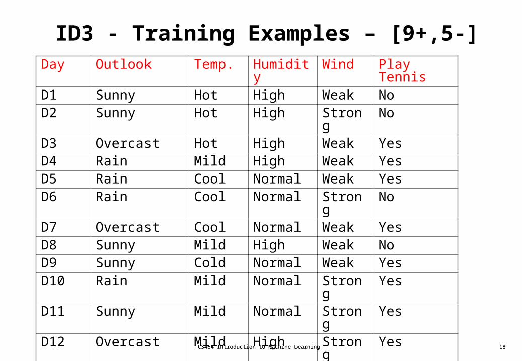
ID3 - Training Examples – [9+,5-]


Day Outlook Temp. Humidity

Wind Play Tennis

D1 Sunny Hot High Weak NoD2 Sunny Hot High Strong NoD3 Overcast Hot High Weak YesD4 Rain Mild High Weak YesD5 Rain Cool Normal Weak YesD6 Rain Cool Normal Strong NoD7 Overcast Cool Normal Weak YesD8 Sunny Mild High Weak NoD9 Sunny Cold Normal Weak YesD10 Rain Mild Normal Strong YesD11 Sunny Mild Normal Strong YesD12 Overcast Mild High Strong YesD13 Overcast Hot Normal Weak YesD14 Rain Mild High Strong No


ID3 – Selecting Next Attribute

Entropy([9+,5-] = – (9/14) log2(9/14) – (5/14) log2(5/14) = 0.940


Humidity

High Normal

[3+, 4-] [6+, 1-]

S=[9+,5-]E=0.940

Gain(S,Humidity) = 0.940-(7/14)*0.985-(7/14)*0.592 = 0.151

E=0.985 E=0.592

Wind

Weak Strong

[6+, 2-] [3+, 3-]

S=[9+,5-]E=0.940

Gain(S,Wind) = 0.940-(8/14)*0.811-(6/14)*1.0 = 0.048




Outlook

Sunny Rain

[2+, 3-] [3+, 2-]

S=[9+,5-]E=0.940

Gain(S,Outlook) = 0.940-(5/14)*0.971 -(4/14)*0.0 -(5/14)*0.0971 = 0.247

E=0.971 E=0.971

Overcast

[4+, 0]

E=0.0




Temp.

Hot Cold

[2+, 2-] [3+, 1-]

S=[9+,5-]E=0.940

Gain(S,Outlook) = 0.940-(4/14)*1.0 - (6/14)*0.911 - (4/14)*0.811 = 0.029

E=1.0 E=0.811

Mild

[4+, 2-]

E= 0.911


Best Attribute - Outlook


Outlook

Sunny Rain

[2+, 3-] [3+, 2-]

S=[9+,5-]S={D1,D2,…,D14}

Overcast

[4+, 0]Ssunny={D1,D2,D8,D9,D11} Sovercast={D3,D7,D12,D13} Srain={D4,D5,D6,D10,D14}

? ? Yes

Which attribute should be tested here?


ID3 - Ssunny


Gain(Ssunny , Humidity) = 0.970-(3/5)0.0 – 2/5(0.0) = 0.970

Gain(Ssunny , Temp.) = 0.970-(2/5)0.0 –2/5(1.0)-(1/5)0.0 = 0.570

Gain(Ssunny , Wind) = 0.970= -(2/5)1.0 – 3/5(0.918) = 0.019

So, Hummudity will be selected


ID3 - Result


Outlook

Sunny Overcast Rain

Humidity

High Normal

Wind

Strong Weak

No Yes

Yes

YesNo

[D3,D7,D12,D13]

[D8,D9,D11] [D6,D14] [D4,D5,D10][D1,D2]


ID3 - AlgorithmID3(Examples, TargetAttribute, Attributes)• Create a Root node for the tree• If all Examples are positive, Return the single-node tree Root, with label = +• If all Examples are negative, Return the single-node tree Root, with label = -• If Attributes is empty, Return the single-node tree Root, with label = most common

value of TargetAttribute in Examples• Otherwise Begin

– A the attribute from Attributes that best classifies Examples– The decision attribute for Root A– For each possible value, vi, of A,

• Add a new tree branch below Root, corresponding to the test A = vi• Let Examplesvi be the subset of Examples that have value vi for A• If Examplesvi is empty

– Then below this new branch add a leaf node with label = most commonvalue of TargetAttribute in Examples

– Else below this new branch add the subtreeID3(Examplesvi , TargetAttribute, Attributes – {A})

• End• Return Root



Hypothesis Space Search in Decision Tree Learning (ID3)

• The hypothesis space searched by ID3 is the set of possible decision trees.

• ID3 performs a simple-to complex, hill-climbing search through this hypothesis space,

• Begins with the empty tree, then considers progressively more elaborate hypotheses in search of a decision tree that correctly classifies the training data.

• The information gain measure guides the hill-climbing search.



Hypothesis Space Search in Decision Tree Learning (ID3)


+ - +

+ - +

A2

-+ - +

A1

- - +

A2

-

A3

A2

-

A4


ID3 - Capabilities and Limitations

• ID3’s hypothesis space of all decision trees is a complete space of finite discrete-valued functions.– Every finite discrete-valued function can be represented by some decision tree.

– Target function is surely in the hypothesis space.

• ID3 maintains only a single current hypothesis, and outputs only a single hypothesis.– ID3 loses the capabilities that follow from explicitly representing all consistent hypotheses.

– ID3 cannot determine how many alternative decision trees are consistent with the available training data.

• No backtracking on selected attributes (greedy search)– Local minimal (suboptimal splits)

• Statistically-based search choices– Robust to noisy data



Inductive Bias in ID3

• ID3 search strategy – selects in favor of shorter trees over longer ones,

– selects trees that place the attributes with highest information gain closest to the root.

– because ID3 uses the information gain heuristic and a hill climbing strategy, it does not always find the shortest consistent tree, and it is biased to favor trees that place attributes with high information gain closest to the root.

Inductive Bias of ID3:

– Shorter trees are preferred over longer trees.

– Trees that place high information gain attributes close to the root are preferred over those that do not.



Inductive Bias in ID3 - Occam’s Razor

OCCAM'S RAZOR: Prefer the simplest hypothesis that fits the data.

Why prefer short hypotheses?

Argument in favor: – Fewer short hypotheses than long hypotheses

– A short hypothesis that fits the data is unlikely to be a coincidence

– A long hypothesis that fits the data might be a coincidence

Argument opposed:– There are many ways to define small sets of hypotheses

– What is so special about small sets based on size of hypothesis



Inductive Bias in ID3 – Restriction Bias and Preference Bias

• ID3 searches a complete hypothesis space – It searches incompletely through this space, from simple to complex hypotheses,

until its termination condition is met

– Its inductive bias is solely a consequence of the ordering of hypotheses by its search strategy.

– Its hypothesis space introduces no additional bias.

• Candidate Elimanation searches an incomplete hypothesis space – It searches this space completely, finding every hypothesis consistent with the

training data.

– Its inductive bias is solely a consequence of the expressive power of its hypothesis representation.

– Its search strategy introduces no additional bias.



Inductive Bias in ID3 – Restriction Bias and Preference Bias

• The inductive bias of ID3 is a preference for certain hypotheses over others, with no hard restriction on the hypotheses that can be eventually enumerated.

preference bias ( search bias ).

• The inductive bias of Candidate Elimination is in the form of a categorical restriction on the set of hypotheses considered.

restriction bias ( language bias )

• A preference bias is more desirable than a restriction bias, because it allows the learner to work within a complete hypothesis space that is assured to contain the unknown target function.



Overfitting

Given a hypothesis space H, a hypothesis hH is said to OVERFIT the training data if there exists some alternative hypothesis h'H, such that h has smaller error than h' over the training examples, but h' has a smaller error than h over the entire distribution of instances.

Reasons for overfitting:

– Errors and noise in training examples

– Coincidental regularities (especially small number of examples are associated with leaf nodes).



Overfitting


• As ID3 adds new nodes to grow the decision tree, the accuracy of the tree measured over the training examples increases monotonically.• However, when measured over a set of test examples independent of the training examples, accuracy first increases, then decreases.


Avoid Overfitting

How can we avoid overfitting?

– Stop growing when data split not statistically significant• stop growing the tree earlier, before it reaches the point where it perfectly

classifies the training data

– Grow full tree then post-prune• allow the tree to overfit the data, and then post-prune the tree.

• The correct tree size is found by stopping early or by post-pruning, a key question is what criterion is to be used to determine the correct final tree size.– Use a separate set of examples, distinct from the training examples, to evaluate the

utility of post-pruning nodes from the tree.

– Use all the available data for training, but apply a statistical test to estimate whether expanding a particular node is likely to produce an improvement beyond the training set. ( chi-square test )



Avoid Overfitting - Reduced-Error Pruning

• Split data into training and validation set

• Do until further pruning is harmful:

– Evaluate impact on validation set of pruning each possible node (plus those below it)

– Greedily remove the one that most improves the validation set accuracy

• Pruning of nodes continues until further pruning is harmful (i.e., decreases accuracy of the tree over the validation set).

• Using a separate set of data to guide pruning is an effective approach provided a large amount of data is available. – The major drawback of this approach is that when data is limited, withholding part

of it for the validation set reduces even further the number of examples available for training.



Effect of Reduced Error Pruning

• the accuracy increases over the test set as nodes are pruned from the tree.

• the validation set used for pruning is distinct from both the training and test sets.


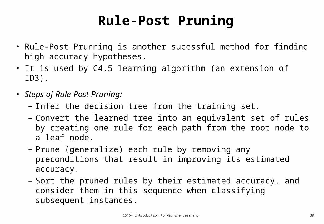
Rule-Post Pruning

• Rule-Post Prunning is another sucessful method for finding high accuracy hypotheses.

• It is used by C4.5 learning algorithm (an extension of ID3).

• Steps of Rule-Post Pruning:

– Infer the decision tree from the training set.

– Convert the learned tree into an equivalent set of rules by creating one rule for each path from the root node to a leaf node.

– Prune (generalize) each rule by removing any preconditions that result in improving its estimated accuracy.

– Sort the pruned rules by their estimated accuracy, and consider them in this sequence when classifying subsequent instances.


Converting a Decision Tree to Rules

Outlook

Sunny Overcast Rain

Humidity

High Normal

Wind

Strong Weak

No Yes

Yes

YesNo

R1: If (Outlook=Sunny) (Humidity=High) Then PlayTennis=No R2: If (Outlook=Sunny) (Humidity=Normal) Then PlayTennis=YesR3: If (Outlook=Overcast) Then PlayTennis=Yes R4: If (Outlook=Rain) (Wind=Strong) Then PlayTennis=NoR5: If (Outlook=Rain) (Wind=Weak) Then PlayTennis=Yes


Pruning Rules

• Each rule is pruned by removing any antecedent (precondition).– Ex. Prune R1 by removing (Outlook=Sunny) or (Humidity=High)

• Select whichever of the pruning steps produced the greatest improvement in estimated rule accuracy.

– Then, continue with other preconditions.

– No pruning step is performed if it reduces the estimated rule accuracy.

• In order to estimate rule accuracy:– use a validation set of examples disjoint from the training set

– evaluate performance based on the training set itself(using statistical techniques). C4.5 uses this approach.


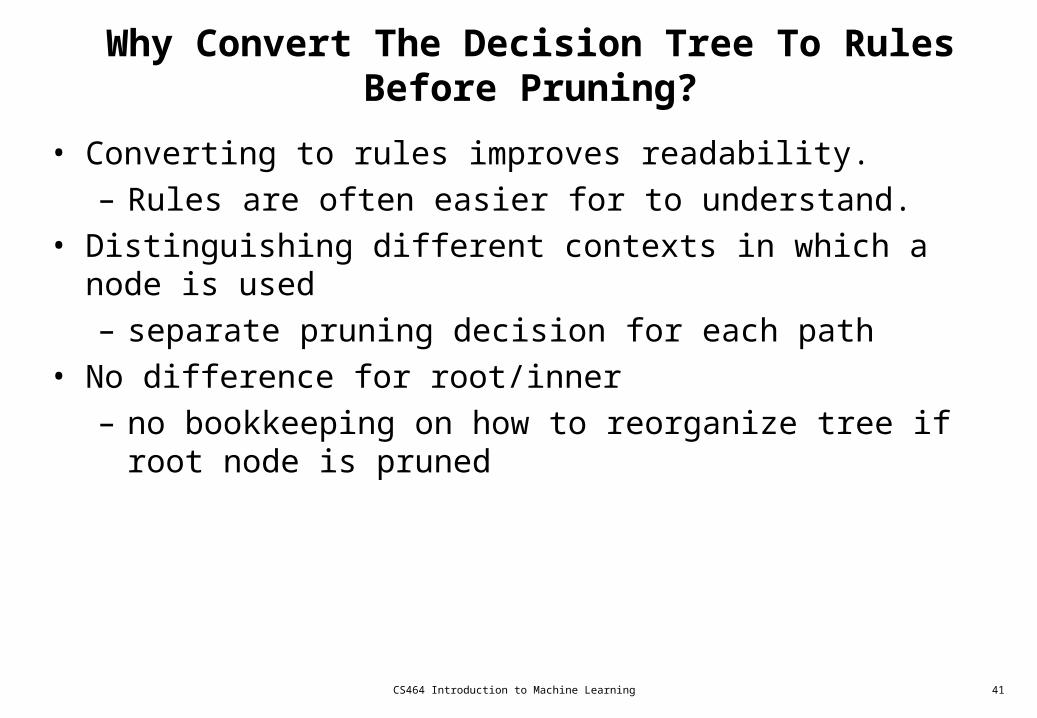
Why Convert The Decision Tree To Rules Before Pruning?

• Converting to rules improves readability.

– Rules are often easier for to understand.

• Distinguishing different contexts in which a node is used

– separate pruning decision for each path

• No difference for root/inner

– no bookkeeping on how to reorganize tree if root node is pruned


Continuous-Valued Attributes

• ID3 is restricted to attributes that take on a discrete set of values.

• Define new discrete valued attributes that partition the continuous attribute value into a discrete set of intervals

• For a continuous-valued attribute A that is, create a new boolean attribute Ac, that is true if A < c and false otherwise.– Select c using information gain

– Sort examples according to the continuous attributeA,

– Then identify adjacent examples that differ in their target classification

– Generate candidate thresholds midway between corresponding values of A.

– The value of c that maximizes information gain must always lie at a boundary.

– These candidate thresholds can then be evaluated by computing the information gain associated with each.


Continuous-Valued Attributes - Example

Temperature: 40 48 60 72 80 90

PlayTennis : No No Yes Yes Yes No

Two candidate thresholds: (48+60)/2=54 (80+90)/2=85

Check the information gain for new boolean attributes:

Temperature>54 Temperature>85

Use these new new boolean attributes same as other discrete valued attributes.


Alternative Selection Measures

• Information gain measure favors attributes with many values– separates data into small subsets

– high gain, poor prediction

• Ex. Date attribute has many values, and may separate training examples into very small subsets (even singleton sets – perfect partitions)– Information gain will be very high for Date attribute.

– Perfect partition maximum gain : Gain(S,Date) = Entropy(S) – 0 = Entropy(S) because log21 is 0.

– It has high information gain, but very poor predictor for unseen data.

• There are alternative selection measures such as GainRatio measure based on SplitInformation


Split Information

• The gain ratio measure penalizes attributes with many values (such as Date) by incorporating a term, called split informution

• Split information for boolean attributes is 1 (= log22),

• Split information fot attributes for n values is log2n

• SplitInformation term discourages the selection of attributes with many uniformly distributed values.

GainRatio(S,A) = Gain(S,A) / SplitInformation(S,A)

i=1

c

SplitInformation(S,A) = - ( |Si| / |S| ) log2 ( |Si| / |S| )


Practical Issues on Split Information

• Some value ‘rules’

– |Si| close to |S|

– SplitInformation 0 or very small

– GainRatio undefined or very large

• Apply heuristics to select attributes

– compute Gain first

– compute GainRatio only when Gain large enough (above average Gain)


Missing Attribute Values

• The available data may be missing values for some attributes.

• It is common to estimate the missing attribute value based on other examples for which this attribute has a known value.

• Assume that an example (with classification c) in S has a missing value for attribute A.– Assign the most common value of A in S.

– Assign the most common value of in the examples having c classification in S.

– Or, use probabilty value for each possibşe attribute value.


Attributes with Differing Costs

• Measuring attribute costs something

– prefer cheap ones if possible

– use costly ones only if good gain

– introduce cost term in selection measure

– no guarantee in finding optimum, but give bias towards cheapest

• Example applications

– robot & sonar: time required to position

– medical diagnosis: cost of a laboratory test


Main Points with Decision Tree Learning

• Decision tree learning provides a practical method for concept learning and for learning other discrete-valued functions. – decision trees are inferred by growing them from the root downward, greedily

selecting the next best attribute.

• ID3 searches a complete hypothesis space.

• The inductive bias in ID3 includes a preference for smaller trees.

• Overfitting training data is an important issue in decision tree learning.– Pruning decision trees or rules are important.

• A large variety of extensions to the basic ID3 algorithm has been developed. These extensions include methods for – post-pruning trees, handling real-valued attributes, accommodating training

examples with missing attribute values, using attribute selection measures other than information gain, and considering costs associated with instance attributes.

CS464 Introduction to Machine Learning1 Decision Tree Learning Decision tree learning is a method...

Documents

Transcript of CS464 Introduction to Machine Learning1 Decision Tree Learning Decision tree learning is a method...