CS177 Lecture 10 Experimental Methods

(PCR, X-ray crystallography, Microarrays)

Tom Madej 11.21.05

Lecture overview

• Polymerase chain reaction (PCR) and its applications.

• X-ray crystallography and the Protein Data Bank (PDB).

• Microarrays and applications.

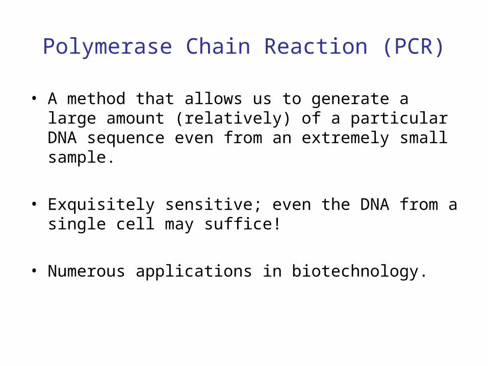
Polymerase Chain Reaction (PCR)

• A method that allows us to generate a large amount (relatively) of a particular DNA sequence even from an extremely small sample.

• Exquisitely sensitive; even the DNA from a single cell may suffice!

• Numerous applications in biotechnology.

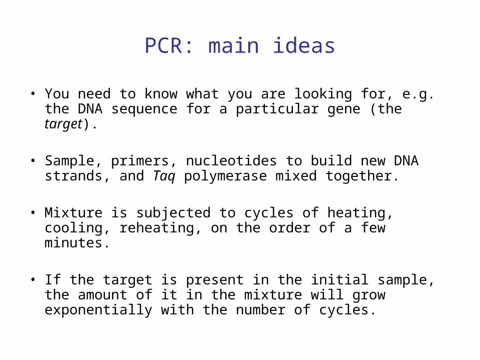
PCR: main ideas

• You need to know what you are looking for, e.g. the DNA sequence for a particular gene (the target).

• Sample, primers, nucleotides to build new DNA strands, and Taq polymerase mixed together.

• Mixture is subjected to cycles of heating, cooling, reheating, on the order of a few minutes.

• If the target is present in the initial sample, the amount of it in the mixture will grow exponentially with the number of cycles.

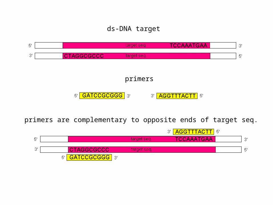
ds-DNA target

primers

primers are complementary to opposite ends of target seq.

PCR cycle

• Mixture is heated to 90ºC for 1-2 minutes to separate the DNA strands (denature).

• Temperature is dropped to 50º-60ºC so that primers can anneal to complementary regions.

• Temperature is raised to 70ºC for 1-2 minutes to allow Taq polymerase to synthesize new DNA strands, starting at the primers; this goes from 5’ to 3’ for both strands.

• Note: The Taq polymerase is a DNA polymerase from Thermus aquaticus, a bacteria that lives in hot springs.

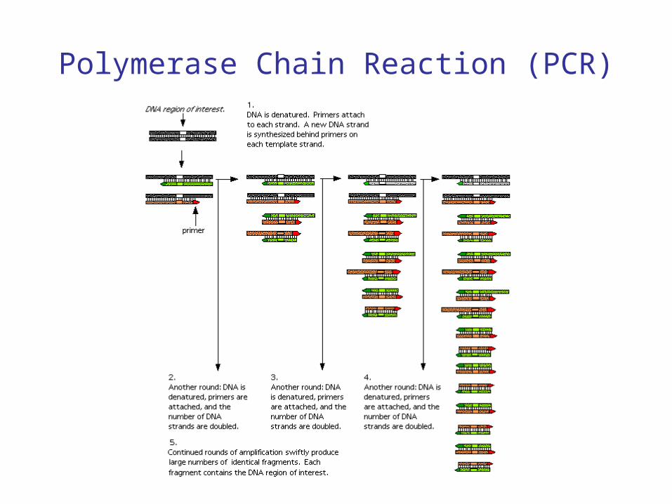
Polymerase Chain Reaction (PCR)

PCR notes

• Primer selection is critical. The primers should be at least 15-20 bases to ensure specificity.

• If you are unsure of the exact sequence, you can use “degenerate” primers, i.e. a mixture of primers (vary at third codon position).

• Note that almost all of the product is exactly the target sequence you want, i.e. with flush ends.

PCR applications

• Making a lot of protein! Use RT-PCR, “reverse transcriptase” PCR, to create DNA with introns removed and then insert it into bacteria to clone the gene. E.g. to make proteins for X-ray crystallography.

• Medical diagnosis: e.g. detect HIV viral proteins long before AIDS symptoms arise; or rapid tuberculosis test.

• Forensics; detect trace amounts of DNA at a crime scene.

Methods to determine protein structures

• X-ray crystallography (most important, over 80% of structures in the PDB are obtained this way).

• NMR spectroscopy (Nuclear Magnetic Resonance).

• Electron microscopy; uses a beam of electrons to create images (maybe issues with sample preparation and resolution in regards to applications to protein structure determination).

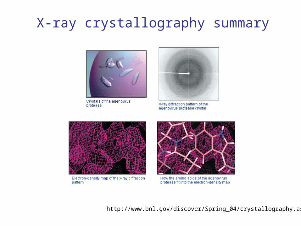
Protein crystallography steps

• Grow crystals of the protein that diffract well (a difficult step, can take from weeks to years!).

• Obtain the X-ray diffraction data.

• Compute electron density maps.

• Refinement: calculate an atomic model to fit electron density; compare the diffraction data computed from the model with the actual data; refine the model to fit the data (iterate).

Protein crystals

http://www-structure.llnl.gov/crystal_lab/Crys_lab.html

Protein crystal

molecule

crystal

The unit cell is the basic unit of symmetry in the crystal.

Facts about protein crystals

• In contrast e.g. to salt or quartz crystals, protein crystals are mostly water (due to the irregular shape of the molecule) and therefore fragile.

• Since they are mostly water, the actual protein structures obtained must be similar to their conformations in vivo.

• To preserve the crystal in the X-ray beam, it is kept at a very low temperature (100ºK).

X-ray diffraction

• The incident beam of X-rays is diffracted by the electrons in the protein molecules in the crystal.

• Some of the diffracted waves will interfere constructively, and others will interfere destructively.

• This results in a diffraction pattern of spots of varying intensity on the detector.

Illustration of diffraction

http://www.eserc.stonybrook.edu/ProjectJava/Bragg/index.html

X-ray diffraction pattern

Analysis of the diffraction pattern

• The diffraction pattern is analyzed by mathematical/computation methods (Fourier analysis) to produce an electron density map.

• This gives a 3-dimensional image of the molecule that will be subjected to further processing and analysis.

Electron density maps at different resolutions

http://www-structure.llnl.gov/Xray/101index.html

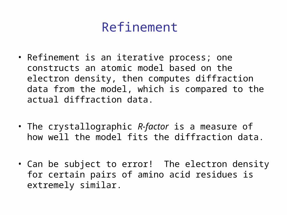
Refinement

• Refinement is an iterative process; one constructs an atomic model based on the electron density, then computes diffraction data from the model, which is compared to the actual diffraction data.

• The crystallographic R-factor is a measure of how well the model fits the diffraction data.

• Can be subject to error! The electron density for certain pairs of amino acid residues is extremely similar.

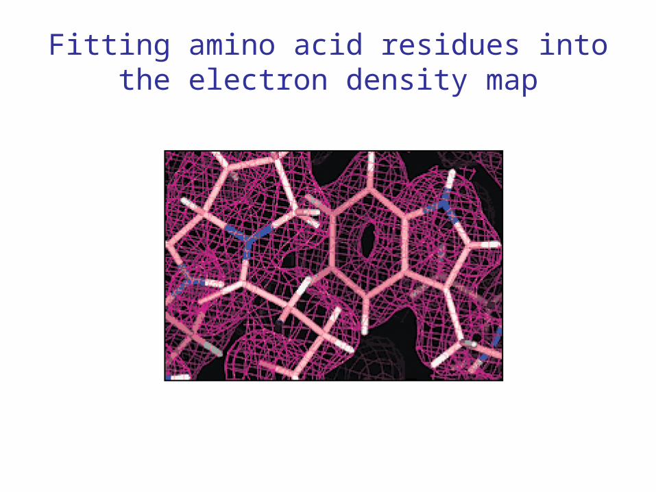
Fitting amino acid residues into the electron density map

http://www.bnl.gov/discover/Spring_04/crystallography.asp

X-ray crystallography summary

NMR

• Based on magnetic moments of atomic nuclei.

• NMR spectra give information about distances between atoms in the molecule.

• Applied to protein molecules in solution (no crystals needed!).

• Only works well for smaller proteins, e.g. 100 residues or less (or so).

• A different set of mathematical/computational tools is involved.

• Note: The different “models” represent different structures compatible with the distance contraints, not actual conformations of the molecule.

PDB

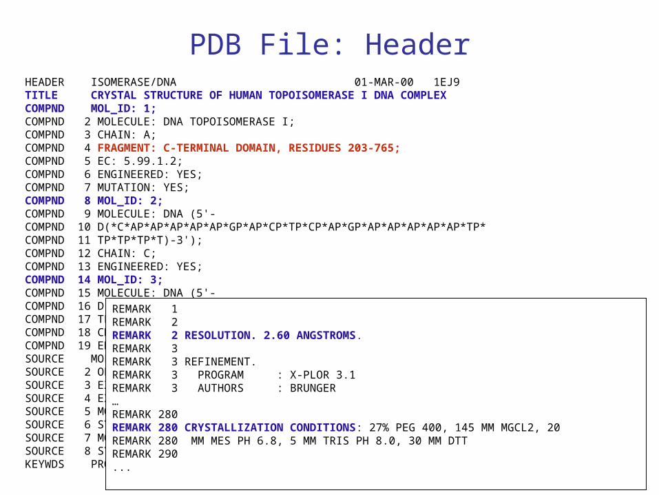
PDB File: HeaderHEADER ISOMERASE/DNA 01-MAR-00 1EJ9TITLE CRYSTAL STRUCTURE OF HUMAN TOPOISOMERASE I DNA COMPLEX COMPND MOL_ID: 1; COMPND 2 MOLECULE: DNA TOPOISOMERASE I; COMPND 3 CHAIN: A; COMPND 4 FRAGMENT: C-TERMINAL DOMAIN, RESIDUES 203-765; COMPND 5 EC: 5.99.1.2; COMPND 6 ENGINEERED: YES; COMPND 7 MUTATION: YES; COMPND 8 MOL_ID: 2; COMPND 9 MOLECULE: DNA (5'- COMPND 10 D(*C*AP*AP*AP*AP*AP*GP*AP*CP*TP*CP*AP*GP*AP*AP*AP*AP*AP*TP* COMPND 11 TP*TP*TP*T)-3'); COMPND 12 CHAIN: C; COMPND 13 ENGINEERED: YES; COMPND 14 MOL_ID: 3; COMPND 15 MOLECULE: DNA (5'- COMPND 16 D(*C*AP*AP*AP*AP*AP*TP*TP*TP*TP*TP*CP*TP*GP*AP*GP*TP*CP*TP* COMPND 17 TP*TP*TP*T)-3'); COMPND 18 CHAIN: D; COMPND 19 ENGINEERED: YES SOURCE MOL_ID: 1; SOURCE 2 ORGANISM_SCIENTIFIC: HOMO SAPIENS; SOURCE 3 EXPRESSION_SYSTEM_COMMON: BACULOVIRUS EXPRESSION SYSTEM; SOURCE 4 EXPRESSION_SYSTEM_CELL: SF9 INSECT CELLS; SOURCE 5 MOL_ID: 2; SOURCE 6 SYNTHETIC: YES; SOURCE 7 MOL_ID: 3; SOURCE 8 SYNTHETIC: YES KEYWDS PROTEIN-DNA COMPLEX, TYPE I TOPOISOMERASE, HUMAN

REMARK 1 REMARK 2 REMARK 2 RESOLUTION. 2.60 ANGSTROMS. REMARK 3 REMARK 3 REFINEMENT. REMARK 3 PROGRAM : X-PLOR 3.1 REMARK 3 AUTHORS : BRUNGER …REMARK 280 REMARK 280 CRYSTALLIZATION CONDITIONS: 27% PEG 400, 145 MM MGCL2, 20 REMARK 280 MM MES PH 6.8, 5 MM TRIS PH 8.0, 30 MM DTT REMARK 290 ...

From Coordinates to Models

1EJ9: Human topoisomerase I

Annotating Secondary Structure

1EJ9: Human topoisomerase I

α-Helices

β-strands

coils/loops

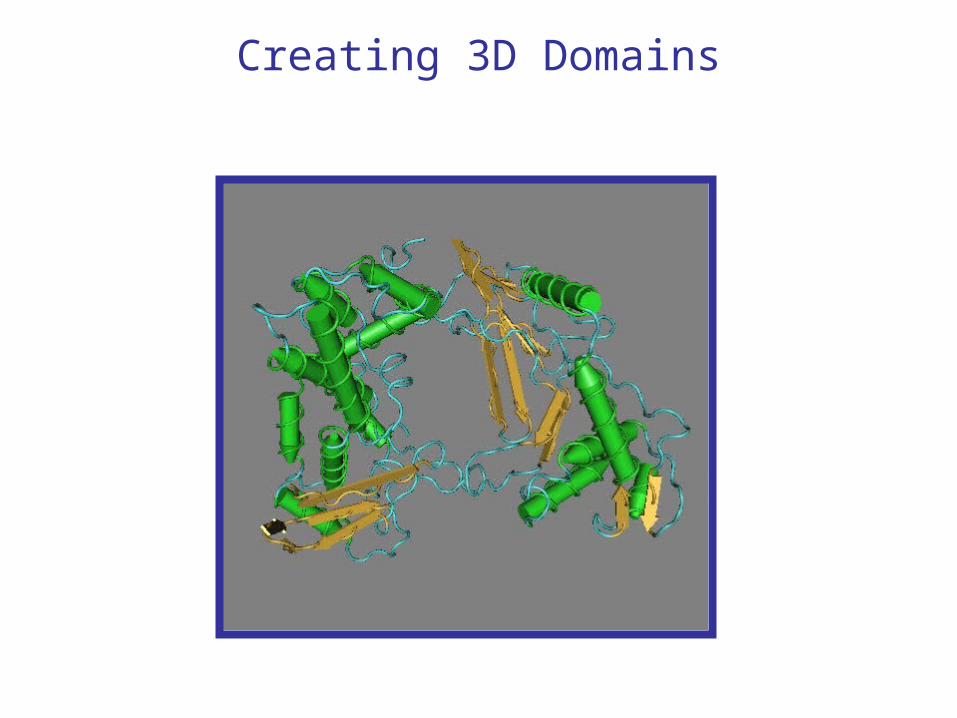
Creating 3D Domains

3D Domain 0: 1EJ9A0 = entire polypeptide

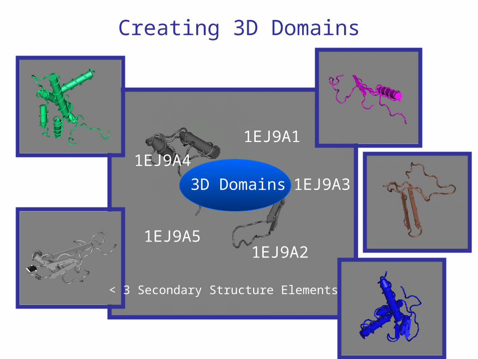
Creating 3D Domains

3D Domains

1EJ9A1

1EJ9A3

1EJ9A2

1EJ9A4

1EJ9A5

< 3 Secondary Structure Elements

Microarrays

• Used to study gene expression levels in cells.

• Cells can differ dramatically in the amounts of various proteins that they synthesize; e.g. due to different cell types or different external/internal conditions.

• In fact, in higher level organisms only a fraction of the genes in a cell are expressed at a given time, and that subset depends on the cell type.

• Via microarrays it is possible to study the expression levels of tens of thousands of genes simultaneously.

Microarray technology

• Physically, a microarray is just a glass slide with spots of DNA on it; each spot is a probe (or target).

• The DNA is single-stranded cDNA (complementary) and may consist of an entire gene or part of one (an oligonucleotide consisting of 50 bases or so).

• If the microarray is exposed to a solution containing mRNA, then the mRNA molecules will bind to those probes to which they are complementary.

Microarray probes

ssDNA genesequences oroligos

Microarray technology

• Thousands of probes can fit on a single slide.

• The slides can be spotted by robots.

• Of course, what genes you can study with a given microarray depends on the collection of probes on it.

• There are a number of commercial manufacturers; e.g. Affymetrix, Agilent, Amersham.

• They’re expensive!

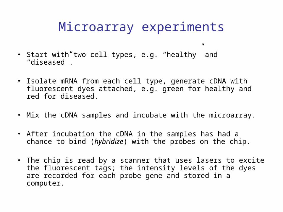
Microarray experiments

• Start with two cell types, e.g. “healthy” and “diseased”.

• Isolate mRNA from each cell type, generate cDNA with fluorescent dyes attached, e.g. green for healthy and red for diseased.

• Mix the cDNA samples and incubate with the microarray.

• After incubation the cDNA in the samples has had a chance to bind (hybridize) with the probes on the chip.

• The chip is read by a scanner that uses lasers to excite the fluorescent tags; the intensity levels of the dyes are recorded for each probe gene and stored in a computer.

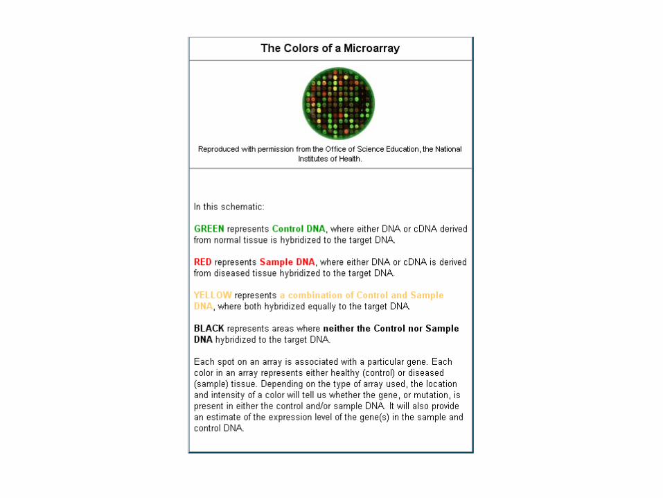
Microarray data representation

• There is a “standard” color scale representation, as follows.

• Red means the gene produced more mRNA in the experimental condition; green means the gene produced more mRNA in the control.

• Black means equal amounts of mRNA for both experiment and control.

• If e.g. there were 5 times as much mRNA for the experimental condition compared to the control, we would say there was a 5-fold induction; 1/5 as much would be 5-fold repression.

• The data is recorded numerically as the log base 2 of the expression ratio.

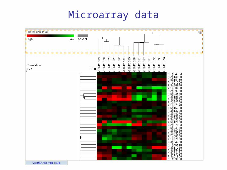
Microarray data

Microarray data analysis

• Since there are typically so many genes, it is useful to cluster the genes based on similar expression patterns.

• Different clustering algorithms may be used, e.g. hierarchical with different metrics, or k-means, k-medians.

• It may also be useful to cluster the samples (we’ll see this shortly).

• Other statistical methods may be useful, e.g. support vector machines (SVM).

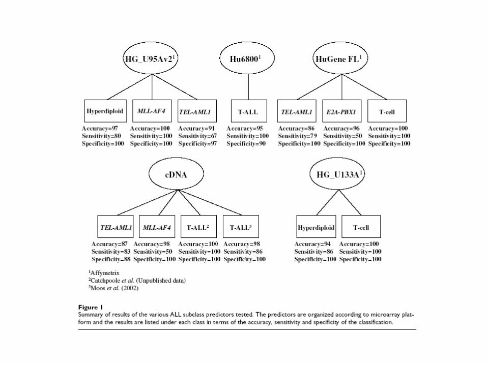
Acute Lymphoblastic Leukemia (ALL)

• Constitutes 75% of annual diagnoses of childhood leukemia.

• Long-term outlook has improved dramatically since about 1970. At that time the long term disease free survival rate (LTDFS) was under 10%; at present it is over 80%.

• There is still a risk of relapse in 20% of patients.

ALL (cont.)

• The LTDFS rate improved because it was recognized that ALL is heterogeneous, and the therapy should be tailored to the subtype so as to improve the odds of a successful treatment (e.g. bone marrow transplant vs. chemotherapy).

• Important subtypes include: T-ALL, E2A-PBX1, BCR-ABL, TEL-AML1, MLL rearrangement, and hyperdiploid > 50 chromosomes.

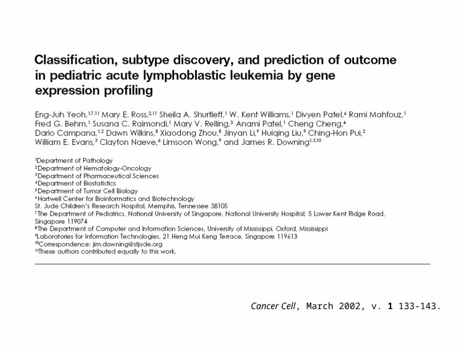
Cancer Cell, March 2002, v. 1 133-143.

Cancer Cell, March 2002, v. 1 133-143.

Cancer Cell, March 2002, v. 1 133-143.

Cancer Cell, March 2002, v. 1 133-143.

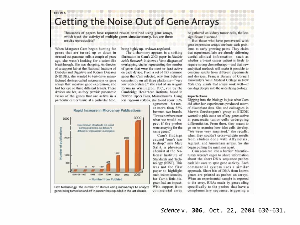
Science v. 306, Oct. 22, 2004 630-631.

Science v. 306, Oct. 22, 2004 630-631.

Abstract from S.A. Mitchell et al.